Asymptotics of extreme statistics of escape time in 1,2 and 3-dimensional diffusions

Abstract

The first of $N$ identical independently distributed (i.i.d.) Brownian trajectories that arrives to a small target, sets the time scale of activation, which in general is much faster than the arrival to the target of only a single trajectory. Analytical asymptotic expressions for the minimal time is notoriously difficult to compute in general geometries. We derive here asymptotic laws for the probability density function of the first and second arrival times of a large number of i.i.d. Brownian trajectories to a small target in 1,2, and 3 dimensions and study their range of validity by stochastic simulations. The results are applied to activation of biochemical pathways in cellular transduction.

1 Introduction

Fast activation of biochemical pathways in cell biology is often initiated by the first arrival of a particle to a small target. This is the case of calcium activation in synapses of neuronal cells [1, 2, 3], fast photoresponse in rods, cones and fly photoreceptors [4, 5, 6], and many more. However, the time scale underlying these fast activations is not very well understood. We propose here that these mechanisms are initiated by the first arrival of one or more of the many identical independently distributed (i.i.d.) Brownian particles to small receptors (such as the influx of many calcium ions inside a synapse to receptors).

In general, one or several particles are required to initiate a cascade of chemical reactions, such as the opening of a protein channel [7] of a cellular membrane, which amplifies the inflow of ions to an avalanche of thousand or more ions, resulting from binding of couple of ions. These statistic of the minimal arrival times are referred to in the statistical physics literature as extreme statistics [8]. Despite great efforts [8, 9, 10, 11, 12, 13, 14, 15, 16], there are no explicit expressions for the probability distributions of arrival times of the first trajectory, the second, and so on. Only general formulas are given, and they account for neither specific geometrical constraints of the bounding domains, where particles evolve, nor for the small targets that bind these particles.

The main example to keep in mind is the statistics of the escape time through a small window of the first of $N$ particles. Asymptotic expressions for the mean escape time of a single Brownian path, the so called narrow escape time, computed in the narrow escape theory [17, 18], depends on global and local geometric properties of the bounding domain and its boundary, such as the surface area (in 2 dimensions or volume (in 3 dimensions), and the local geometry near the absorbing window (mean curvature of the boundary at the small window, the window’s shape, and relative size). The number and distribution of absorbing windows can influence drastically the narrow escape time. As shown below, the escape of the fastest particles selects trajectories that are very different from the typical ones, which determine the mean narrow escape time (NET).

Moreover, the asymptotics of the expected first arrival time are not the same as of the mean first passage time (MFPT) of a single Brownian path to a small window. The analysis relies on the time-dependent solution of the Fokker-Planck equation and the short-time asymptotics of the survival probability. Previous studies of the short-time asymptotics of the diffusion equation concern the asymptotics of the trace of the heat kernel analysis [19, 20]. Here, an estimate is needed of the survival probability, which requires different analysis. Our method is based on the construction of the asymptotics from Green’s function of the Helmholtz equation.

The main results are explicit expressions for the statistics of the first arrival time see attempt in [14]) in 1,2, and 3 dimensions and a formula for the expected shortest exit time from a neuronal spine with and without returns. The manuscript is organized as follows. First we present the general framework for the computation of the pdf of the first arrival and conditional second arrival, given that the first one has already arrived, in a population of $N$ Brownian particles in a ray and in an interval. We then study the difference between Poissonian and diffusion escape time approximations and in particular, we consider the case of a bulk domain with a window connected to a narrow cylinder (dendritic spine shape [17, 18]). We then compute the pdf of the extreme escape time in dimensions 2 and 3 through small windows. Finally, we discuss applications to activation in cellular biology.

2 The pdf of the first escape time

The narrow escape problem (NEP) for the shortest arrival time of $N$ non-interacting i.i.d. Brownian trajectories (ions) in a bounded domain $\Omega$ to a binding site is defined as follows. Denote by $t_{i}$ the arrival times and by $\tau^{1}$ the shortest one,

$$\tau^{1}=\min(t_{1},\ldots,t_{N}),$$ (1)

where $t_{i}$ are the i.i.d. arrival times of the $N$ ions in the medium. The NEP is to find the PDF and the MFPT of $\tau^{1}$. The complementary PDF of $\tau^{1}$ is given by

$$\Pr\{\tau^{1}>t\}={\Pr}^{N}\{t_{1}>t\},$$ (2)

where $\Pr\{t_{1}>t\}$ is the survival probability of a single particle prior to binding at the target. This probability can be computed from the following boundary value problem. Assuming that the boundary $\partial\Omega$ contains $N_{R}$ binding sites $\partial\Omega_{i}\subset\partial\Omega\ (\partial\Omega_{a}=\bigcup\limits_{i=1}^{N_{R}}\partial\Omega_{i},\ \partial\Omega_{r}=\partial\Omega-\partial\Omega_{a})$, the pdf of a Brownian trajectory is the solution of the initial boundary value problem (IBVP)

$$\frac{\partial p(\mbox{\boldmath$x$},t)}{\partial t}= D\Delta p(\mbox{\boldmath$x$},t)\quad\hbox{\rm for }\mbox{\boldmath$x$}\in\Omega,\ t>0$$ (3)

$$p(\mbox{\boldmath$x$},0)= p_{0}(\mbox{\boldmath$x$})\quad\hbox{\rm for }\mbox{\boldmath$x$}\in\Omega$$

$$\frac{\partial p(\mbox{\boldmath$x$},t)}{\partial\mbox{\boldmath$n$}}= 0\quad\hbox{\rm for }\mbox{\boldmath$x$}\in\partial\Omega_{r}$$

$$p(\mbox{\boldmath$x$},t)= 0\quad\hbox{\rm for }\mbox{\boldmath$x$}\in\partial\Omega_{a}.$$

The survival probability is

$$\Pr\{t_{1}>t\}=\int\limits_{\Omega}p(\mbox{\boldmath$x$},t)\,d\mbox{\boldmath$x$},$$ (4)

so that

$$\Pr\{\tau^{1}=t\}=\frac{d}{dt}\Pr\{\tau^{1}<t\}=N(\Pr\{t_{1}>t\})^{N-1}\Pr\limits\{t_{1}=t\},$$ (5)

where

$$\Pr\{t_{1}=t\}=\oint\limits_{\partial\Omega_{a}}\frac{\partial p(\mbox{\boldmath$x$},t)}{\partial\mbox{\boldmath$n$}}\,dS_{\mbox{\boldmath$x$}}.$$ (6)

$$\Pr\{t_{1}=t\}=N_{R}\oint\limits_{\partial\Omega_{1}}\frac{\partial p(\mbox{\boldmath$x$},t)}{\partial\mbox{\boldmath$n$}}\,dS_{\mbox{\boldmath$x$}}.$$ (7)

Putting all the above together results in the pdf

$$\Pr\{\tau^{1}=t\}=NN_{R}\left[\int\limits_{\Omega}p(\mbox{\boldmath$x$},t)d\mbox{\boldmath$x$}\right]^{N-1}\oint\limits_{\partial\Omega_{1}}\frac{\partial p(\mbox{\boldmath$x$},t)}{\partial\mbox{\boldmath$n$}}dS_{\mbox{\boldmath$x$}}.$$ (8)

The first arrival time is computed from the survival probability of a particle and the flux through the target. Obtaining an explicit or asymptotic expression is not possible in general.

2.1 The pdf of the first arrival time in an interval

To obtain an analytic expression for the pdf of the first arrival time (8) of a particle inside a narrow neck that could represent the dendritic spine neck, we model the narrow spine neck as a segment of length $L$, with a reflecting boundary at $x=0$ and absorbing boundary at $x=L$. Then the diffusion boundary value problem (3) becomes

$$\displaystyle{\frac{\partial p}{\partial t}}= \displaystyle{D\frac{\partial^{2}p}{\partial x^{2}}}\quad\mbox{ for}\ 0<x<L,\ t>0$$ (9)

$$p(x,0)= \delta(x)\quad\mbox{ for}\ 0<x<L$$ (10)

$$p(L,t)= \frac{\partial p(0,t)}{\partial x}=0\quad\hbox{ for }t>0,$$ (11)

where the initial condition corresponds to a particle initially at the origin. The general solution is given by the eigenfunction expansion

$$p(x,t)=2\sum^{\infty}_{n=0}e^{-D\lambda^{2}_{n}t}\cos\lambda_{n}x,$$ (12)

where the eigenvalues are

$$\lambda_{n}=\frac{\pi}{L}\left(n+\frac{1}{2}\right).$$ (13)

The survival probability (4) of a particle is thus given by

$$\Pr\{t_{1}>t\}=\int\limits_{0}^{L}p(x,t)dx=2\sum^{\infty}_{n=0}\frac{(-1)^{n}}{\lambda_{n}}e^{-D\lambda^{2}_{n}t}.$$ (14)

The pdf of the arrival time to $L$ of a single Brownian trajectory is the probability efflux at the absorbing boundary $\partial\Omega_{a}$, given by

$$-\oint\limits_{\Omega_{a}}\frac{\partial p(\mbox{\boldmath$x$},t)}{\partial\mbox{\boldmath$n$}}\,dS_{\mbox{\boldmath$x$}}=-\frac{\partial p(L,t)}{\partial x}=2\sum^{\infty}_{n=0}{(-1)^{n}}{\lambda_{n}}e^{-D\lambda^{2}_{n}t}.$$ (15)

Therefore, the pdf of the first arrival time in an ensemble of $N$ particles to one of $N_{R}$ independent absorbers is given by

$$\Pr\{\tau^{(1)}=t\}=2NN_{R}\left(2\sum^{\infty}_{n=0}\frac{(-1)^{n}}{\lambda_{n}}e^{-D\lambda^{2}_{n}t}\right)^{N-1}\sum^{\infty}_{n=0}{(-1)^{n}}{\lambda_{n}}e^{-D\lambda^{2}_{n}t}.$$ (16)

For numerical purposes, we approximate (16) by the sum of $n_{0}$ terms,

$$\Pr\{\tau^{(1)}=t\}\approx f_{n_{0}}(t)=NN_{R}\left(\sum^{n_{0}}_{n=0}\frac{(-1)^{n}}{\lambda_{n}}e^{-D\lambda^{2}_{n}t}\right)^{N-1}\sum^{n_{0}}_{n=0}{(-1)^{n}}{\lambda_{n}}e^{-D\lambda^{2}_{n}t}.$$ (17)

Figs.1A-B show the pdf of the first arrival time for $N=5$ and $N=500$ Brownian particles with diffusion coefficient $D=1$, which start at $x=0$ at time 0 and exit the interval at $x=1$. These figures confirm the validity of the analytical approximation (16) with only $n_{0}=100$ terms in the lowly converging alternating series.

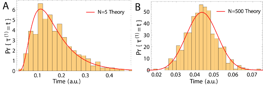
Figure 1: Histograms of the arrival times to the boundary of the fastest particle, obtained from Brownian simulations with Euler’s scheme. The number of Brownian particles is $N=5$ in A and $N=500$ in B. The analytical solution (red curves) is obtained by setting $n_{0}=100$ in (17).

3 Statistics of the arrival time of the second particle

Next, we turn to the computation of the conditional pdf of the arrival time $\tau^{(2)}$ of the second particle, which is that of the minimum of the shortest arrival time in the ensemble of $N-1$ trajectories after the first one has arrived, conditioned on their locations at time $\tau^{(1)}$. The time $\tau^{(1)}+\tau^{(2)}$ is that of arrival of the first two particles at reach the target. The conditional distribution of the arrival time $\tau^{(2)}$ of the second particle, given the positions of the $N-1$ particles at time $\tau^{(1)},$ can be computed from their joint probability distribution at positions $(x_{1},\ldots,x_{N-1})$ and the first particle has already arrived at time $\tau^{(1)}=s$,

$$\Pr\{\tau^{(2)}=t\}$$

$$= \int_{0}^{t}\int_{\Omega}..\int_{\Omega}\Pr\{\tau^{(2)}=t,\tau^{1}=s,\mbox{\boldmath$x$}_{1}(s)=x_{1},\ldots,\mbox{\boldmath$x$}_{N-1}(s)=x_{N-1}\}\,dx_{1}\cdots\,dx_{N}\,ds$$

and

$$\Pr\{\tau^{(2)}=t,\tau^{1}=s,x_{1}(s)=x_{1},\ldots,x_{N-1}(s)=x_{N-1}\}$$

$$= \Pr\{\tau^{(2)}=t\,|\,\tau^{1}=s,x_{1}(s)=x_{1},\ldots,x_{N-1}(s)=x_{N-1}\}$$

$$\times\Pr\{\tau^{1}=s\}\Pr\{x_{1}(s)=x_{1},\ldots,x_{N-1}(s)=x_{N-1}\}.$$

Because all particles are independent,

$$\Pr\{\mbox{\boldmath$x$}_{1}(s)=x_{1},\ldots,\mbox{\boldmath$x$}_{N-1}(s)=x_{N-1}\}=\prod_{i=1}^{N-1}\Pr\{\mbox{\boldmath$x$}_{i}(s)=x_{i}\}$$

so that

$$\Pr\{\tau^{(2)}=t\}=\int\limits_{0}^{t}\Pr\{\tau^{(2)}=t\,|\,\tau^{1}=s\}\left(\int\limits_{0}^{L}\Pr\{\mbox{\boldmath$x$}_{1}(s)=x_{1}\}dx_{1}\right)^{N}\Pr\{\tau^{1}=s\}ds.$$ (19)

3.1 The Poissonian-like approximation

The pdf (19) can be evaluated under some additional assumptions. For example, if the Brownian trajectories escape from a deep potential well, the escape process is well approximated by a Poisson process with rate equal the reciprocal of the mean escape time from the well [21]. Also, when Brownian particles escape a domain $\Omega=B\cup C$, which consists of a bulk $B$ and a narrow cylindrical neck $C$, the escape process from $\Omega$ can be approximated by a Poisson process, according to the narrow scape theory [17]. Here the motion in the narrow cylinder $C$ is approximated by one-dimensional Brownian motion in an interval of length $L$.

Consequently, under the Poisson approximation, the arrival of the first particle is much faster than the escape of the second one from the bulk compartment $B$, thus we can use the approximation that all particles are still in the bulk $B$ after the arrival of the first one. The bulk is represented by the position $x=0$ in an approximate one-dimensional model. This assumption simplifies (19) to

$$\left(\int\limits_{0}^{L}\Pr\{\mbox{\boldmath$x$}_{1}(s)=x_{1}\}dx_{1}\right)^{N}\approx 1,$$ (20)

so that

$$\Pr\{\tau^{(2)}=t\}=\int\limits_{0}^{t}\Pr\{\tau^{(2)}=t|\tau^{1}=s\}\Pr\{\tau^{1}=s\}ds.$$ (21)

The Markovian property of the Poisson process gives

$$\Pr\{\tau^{(2)}=t|\tau^{1}=s\}=\Pr\{\tau^{(2)}=t-s,\}$$ (22)

so that $\tau^{(2)}$ has the same pdf as $\tau^{1}$ with $N-1$ particles, which we approximate to be the same for large $N$, that is,

$$\Pr\{\tau^{(2)}=t\}=\int\limits_{0}^{t}f(t-s)f(s)\,ds,$$ (23)

where (recall (16))

$$f(s)=\Pr\{\tau^{1}=s\}=NN_{R}g(t)^{N}h(t).$$ (24)

In one dimension, $g(t)=\sum^{N_{t}}_{n=0}\frac{(-1)^{n}}{\lambda_{n}}e^{-D\lambda^{2}_{n}t}$ and $h(t)=\sum^{N_{t}}_{n=0}{(-1)^{n}}{\lambda_{n}}e^{-D\lambda^{2}_{n}t}$. It follows that

$$\Pr\{\tau^{(2)}=t\}\approx N^{2}N_{R}^{2}\int\limits_{0}^{t}g(s)^{N-1}h(s)g(t-s)^{N-1}h(t-s)ds.$$ (25)

3.2 $\Pr\{\tau^{(2)}\}$ of $N$ Brownian i.i.d. trajectories in a segment

As in the first paragraph of section 3, equations (3) and (19) are valid with $\Omega$ replaced by the segment $[0,L]$. That is,

$$\Pr\{\tau^{(2)}=t\}$$

$$= \int\limits_{0}^{t}\int\limits_{0}^{L}\cdots\int\limits_{0}^{L}\Pr\{\tau^{(2)}=t,\tau^{1}=s,x_{2}(s)=x_{2},\ldots,x_{N}(s)=x_{N}\}\,dx_{2}\cdots\,dx_{N}\,ds.$$

and

$$\Pr\{\tau^{(2)}=t,\tau^{1}=s,x_{2}(s)=x_{1},\ldots,x_{N-1}(s)=x_{N}\}$$

$$= \Pr\{\tau^{(2)}=t|\tau^{1}=s,x_{2}(s)=x_{1},\ldots,x_{N-1}(s)=x_{N}\}$$

$$\times\Pr\{\tau^{1}=s\}\Pr\{x_{2}(s)=x_{1},\ldots,x_{N-1}(s)=x_{N}\}.$$

Because all particles are independent,

$$\Pr\{x_{2}(s)=x_{1},\ldots,x_{N}(s)=x_{N-1}\}=\prod_{i=1}^{N-1}\Pr\{x_{i+1}(s)=x_{i}\},$$ (26)

hence,

$$\Pr\{\tau^{(2)}=t\}=\int\limits_{0}^{t}\Pr\{\tau^{(2)}=t|\tau^{1}=s\}\left(\int\limits_{0}^{L}\Pr\{x_{1}(s)=x_{1}\}dx_{1}\right)^{N-1}\Pr\{\tau^{1}=s\}\,ds.$$ (27)

To compute the survival probability

$$S(s)=\int\limits_{0}^{L}\Pr\{x_{1}(s)=x_{1}\}\,dx_{1},$$ (28)

we use the short-time asymptotics of the one-dimensional diffusion equation. Modifying equation (9) for short-time diffusion of a particle starting at $0$, we get

$$\frac{\partial p(x,t)}{\partial t}= D\frac{\partial^{2}p(x,t)}{\partial x^{2}}\quad\mbox{for}\ x>0,\ t>0$$

$$p(x,0)= \delta(x)\quad\mbox{for}\ x>0,\quad p(L,t)=0\quad\mbox{for}\ t>0.$$ (29)

The short-time diffusion is well approximated by the fundamental solution (except at the boundary, where the error is exponentially small in $1/t$)

$$p(x,t)=\frac{1+o(t)}{\sqrt{4D\pi t}}\exp\left\{-\frac{x^{2}}{4Dt}\right\}.$$ (30)

Thus the survival probability at short time $t$ is

$$S(t)=\int\limits_{0}^{L}\frac{1+o(t)}{\sqrt{4D\pi t}}\exp\left\{-\frac{x^{2}}{4Dt}\right\}\,dx.$$ (31)

The short-time asymptotic expansion (42) (see below) and the change of variable $x=u\sqrt{4Dt}$ in the integral (31), give

$$S(t) = 1-\frac{1}{\sqrt{\pi}}\int\limits^{\infty}_{L/\sqrt{4Dt}}\left[\exp\left\{-u^{2}\right\}\right]du$$ (32)

$$\approx 1-\sqrt{4Dt}\frac{\exp\left\{-(L/\sqrt{4Dt})^{2}\right\}}{\sqrt{\pi}L}\left(1-2\frac{Dt}{L^{2}}+O\left(\frac{t^{2}}{L^{4}}\right)\right).$$ (33)

It follows from (27) that the pdf of the second arrival time is

$$\Pr\{\tau^{(2)}=t\}$$

$$= [1+o(1)]\int\limits_{0}^{t}\Pr\{\tau^{1}=s\}\Pr\{\tau^{1}=t-s\}\left(1-\sqrt{4Ds}\frac{\exp\left\{-(\frac{L}{\sqrt{4Ds}})^{2}\right\}}{\sqrt{\pi}L}\right)^{N-1}\,ds.$$

Figure 2 compares results of the stochastic simulations with the analytical formula (25) for the second fastest arrival time $\tau^{(2)}$ to the boundary 1 of the interval $[0,1]$ among 20 particles. We use the analytical formula (25) (no correction) and (3.2), which contains the shift correction due to the distribution of the particles in the interval at time $\tau^{(1)}$, when the first particle arrives at $x=L$ been absorbed.

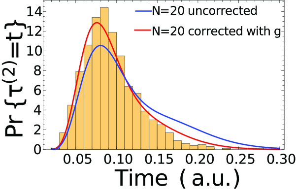
Figure 2: Histogram of the arrival time of the second fastest particle, obtained from Brownian simulations with Euler’s scheme. The fastest is computed for $N=20$ in B. The analytical solution with no correction is given by (22) (blue) and compared to (3.2) with the correction (red). There are $n_{0}=6$ terms in the series (17).

This figure shows how the corrected formula gives a better agreement with the Brownian simulations, thus proving that the distribution of the Brownian particles inside the interval contributes to the decrease of the arrival time of the second particle. The fit to simulation data is based on the eigenfunction expansion

$$\Pr\{\tau^{(2)}=t\}=[1+o(1)]\int\limits_{0}^{t}\Pr\{\tau^{1}=s\}\Pr\{\tau^{1}=t-s\}\left(2\sum^{\infty}_{n=0}\frac{(-1)^{n}}{\lambda_{n}}e^{-D\lambda^{2}_{n}t}\right)^{N-1}ds,$$ (35)

which is equivalent to (3.2). Formula (24) is used for $\Pr\{\tau^{1}=s\}$. Note that the alternating series contains an even number of terms.

To conclude, the internal distribution of particle is given by

$$\left(1-\sqrt{4Ds}\frac{\exp\left\{-(\frac{L}{\sqrt{4Ds}})^{2}\right\}}{\sqrt{\pi}L}\right)^{N-1}$$

and causes the faster arrival of the second particle relative to the first one. This example shows the deviation from the purely Poissonian approximation.

4 Asymptotics of the expected shortest time $\bar{\tau}^{1}$

The MFPT of the first among $N$ i.i.d. Brownian paths is given by

$$\bar{\tau}^{1}=\int\limits\limits_{0}^{\infty}\Pr\{\tau^{1}>t\}dt=\int\limits_{0}^{\infty}\left[\Pr\{t_{1}>t\}\right]^{N}dt,$$ (36)

where $t_{1}$ is the arrival time of a single Brownian path. Writing the last integral in (36) as

$$\bar{\tau}^{1}=\int\limits_{0}^{\infty}e^{N\ln g(t)}dt,$$ (37)

it can be expanded for $N\gg 1$ by Laplace’s method. Here

$$g(t)=\sum^{\infty}_{n=0}\frac{(-1)^{n}}{\lambda_{n}}e^{-D\lambda^{2}_{n}t}$$ (38)

(see (14)).

4.1 Escape from a ray

Consider the case $L=\infty$ and the IBVP

$$\frac{\partial p(x,t)}{\partial t} = D\frac{\partial^{2}p(x,t)}{\partial x^{2}}\quad\mbox{ for }x>0,\ t>0$$

$$p(x,0) = \delta(x-a)\quad\mbox{ for }\ x>0,\quad p(0,t)=0\quad\mbox{ for }t>0,$$ (39)

whose solution is

$$p(x,t)=\frac{1}{\sqrt{4D\pi t}}\left[\exp\left\{-\frac{(x-a)^{2}}{4Dt}\right\}-\exp\left\{-\frac{(x+a)^{2}}{4Dt}\right\}\right].$$ (40)

The survival probability with $D=1$ is

$$\Pr\{t_{1}>t\}=\int\limits\limits_{0}^{\infty}p(x,t)\,dx=1-\frac{2}{\sqrt{\pi}}\int\limits\limits_{a/\sqrt{4t}}^{\infty}e^{-u^{2}}\,du.$$ (41)

To compute the MFPT in (36), we use the expansion of the complementary error function

$$\frac{2}{\sqrt{\pi}}\int\limits\limits_{x}^{\infty}e^{-u^{2}}\,du=\frac{e^{-x^{2}}}{x\sqrt{\pi}}\left(1-\frac{1}{2x^{2}}+O(x^{-4})\right)\quad\mbox{for}\ x\gg 1,$$ (42)

which gives

$$I_{N}\equiv\int\limits\limits_{0}^{\infty}\left[\Pr\{t_{1}>t\}\right]^{N}dt\approx\int\limits\limits_{0}^{\infty}\exp\left\{N\ln\left(1-\frac{e^{-(a/\sqrt{4t})^{2}}}{(a/\sqrt{4t})\sqrt{\pi}}\right)\right\}\,dt,$$ (43)

and with the approximation

$$I_{N}\approx\int\limits\limits_{0}^{\infty}\exp\left\{-N\frac{\sqrt{4t}e^{-\frac{a^{2}}{4t}}}{a\sqrt{\pi}}\right\}\,dt=\frac{a^{2}}{4}\int\limits\limits_{0}^{\infty}\exp\left\{-N\frac{\sqrt{u}e^{-\frac{1}{u}}}{\sqrt{\pi}}\right\}du.$$ (44)

To evaluate the integral (44), we make the monotone change of variable

$$w=w(t)=\sqrt{t}e^{-1/t},\quad w^{\prime}(t)=\sqrt{t}e^{-\frac{1}{t}}\left(\frac{1}{2t}+\frac{1}{t^{2}}\right).$$ (45)

Note that for small $t$,

$$w^{\prime}(t)\approx w\frac{1}{t^{2}}$$ (46)

and $\ln w\approx-1/t$. Thus,

$$w^{\prime}(t)\approx w(\ln w)^{2}.$$ (47)

Breaking with $N^{\prime}=\frac{N}{\sqrt{\pi}}$

$$I_{N} \approx \frac{a^{2}}{4}\int\limits_{0}^{\infty}\exp\{-N^{\prime}w\}\frac{1}{\frac{dw}{dt}}\,dw$$

$$\approx \frac{a^{2}}{4}\left(\int\limits\limits_{0}^{\delta}\exp\{-N^{\prime}w\}\frac{a^{2}}{w(\ln(w))^{2}}\,dw+\int\limits\limits_{\delta}^{\infty}\exp\{-N^{\prime}w\}\frac{1}{\frac{dw}{dt}}\,dw\right)$$

for some $0<\delta<1$, the second integral turns out to be exponentially small in $N$ and is thus negligible relative to the first one. Integrating by parts,

$$I_{N} \approx \frac{a^{2}}{4}\int\limits_{0}^{\delta}\exp\{-N^{\prime}w\}\frac{1}{w(\ln(w))^{2}}dw$$

$$\approx O(\exp(-aN))+\frac{a^{2}}{4}N^{\prime}\int\limits_{0}^{\delta}\exp\{-N^{\prime}w\}\frac{1}{\ln|w|\,}dw$$

and changing the variable to $u=N^{\prime}w$, we obtain

$$N^{\prime}\int\limits\limits_{0}^{\delta}\exp\{-N^{\prime}w\}\frac{a^{2}}{4\ln|w|}\,dw=\int\limits_{0}^{N^{\prime}\delta}\frac{a^{2}\exp\{-u\}}{4|\ln u/N^{\prime}|}\,du.$$

Expanding

$$\frac{1}{|\ln u/N^{\prime}|}=\frac{1}{\ln N^{\prime}}\left(1+\frac{|\ln u|}{\ln N}+O\left(\frac{|\ln u|}{\ln N^{\prime}}\right)^{2}\right)$$

for $u>\varepsilon>0$, we obtain,

$$N^{\prime}\int\limits\limits_{0}^{\delta}\exp\{-N^{\prime}w\}\frac{a^{2}}{4\ln w}dw\approx\int\limits\limits_{0}^{N^{\prime}\delta}\exp\{-u\}\frac{a^{2}}{4|\ln N^{\prime}|}\left(1+\frac{|\ln u|}{\ln N^{\prime}}\right)du.$$

Thus, breaking the integral into two parts, from $[0,\varepsilon]$ (which is negligible) and $[\varepsilon,\infty[$, we get

$$\bar{\tau}^{1}\approx\frac{a^{2}}{4D\ln\frac{N}{\sqrt{\pi}}}\quad\mbox{for}\ N\gg 1.$$ (48)

4.2 Escape for the second fastest from half a line

Equation (23) and the approximation (20) give

$$\Pr\{\tau^{(2)}=t\}=\int\limits_{0}^{t}f(t-s)f(s)\,ds,$$ (49)

where

$$f(s)=\Pr\{\tau^{1}=s\}=NN_{R}g(t)^{N}h(t).$$ (50)

According to (41),

$$g(t)=\Pr\{t_{1}>t\}=\int\limits\limits_{0}^{\infty}p(x,t)\,dx=1-\frac{2}{\sqrt{\pi}}\int\limits\limits_{a/\sqrt{4t}}^{\infty}e^{-u^{2}}\,du\approx 1-\frac{e^{-(a/\sqrt{4t})^{2}}}{(a/\sqrt{4t})\sqrt{\pi}}$$ (51)

and

$$h(t)=-\frac{d\Pr\{t_{1}>t\}}{dt}=\frac{2}{\sqrt{\pi}}\frac{a^{2}}{4\sqrt{t^{3}}}e^{-(a/\sqrt{4t})^{2}}.$$ (52)

The MFPT of the second arrival is obtained from (49) as

$$\bar{\tau}^{(2)} = \int\limits_{0}^{\infty}t\Pr\{\tau^{(2)}=t\}dt=\int\limits_{0}^{\infty}t\int\limits_{0}^{t}f(t-s)f(s)dsdt$$ (53)

$$= 2\int\limits_{0}^{\infty}sf(s)ds\left(\int\limits_{0}^{\infty}f(t)dt\right)=2\bar{\tau}^{(1)}\left(\int\limits_{0}^{\infty}f(t)dt\right)=2\bar{\tau}^{(1)}.$$ (54)

5 Escape from an interval $[0,a]$

We follow the steps of the previous section, where Green’s function for the homogenous IBVP is now given by the infinite sum

$$p(x,t\,|\,y)=\frac{1}{\sqrt{4D\pi t}}\sum\limits_{n=-\infty}^{\infty}\left[\exp\left\{-\frac{(x-y+2na)^{2}}{4t}\right\}-\exp\left\{-\frac{(x+y+2na)^{2}}{4t}\right\}\right].$$ (55)

The conditional survival probability is

$$\Pr\{t_{1}>t\,|\,y\}= \int\limits\limits_{0}^{a}p(x,t\,|\,y)\,dx$$ (56)

$$= \frac{1}{\sqrt{4D\pi t}}\sum\limits_{n=-\infty}^{\infty}\int\limits\limits_{0}^{a}\left[\exp\left\{-\frac{(x-y+2na)^{2}}{4t}\right\}-\exp\left\{-\frac{(x+y+2na)^{2}}{4t}\right\}\right]\,dx$$

$$= \int\limits\limits_{0}^{a}\frac{1}{\sqrt{4D\pi t}}\left[\exp\left\{-\frac{(x-y)^{2}}{4t}\right\}-\exp\left\{-\frac{(x+y)^{2}}{4t}\right\}\right]\,dx+S_{1}(y,t)-S_{2}(y,t),$$

where

$$S_{1} = \frac{1}{\sqrt{4D\pi t}}\sum\limits_{n=1}^{\infty}\int\limits\limits_{0}^{a}\left[\exp\left\{-\frac{(x+y+2na)^{2}}{4t}\right\}-\exp\left\{-\frac{(x-y+2na)^{2}}{4t}\right\}\right]\,dx$$

$$S_{2} = \frac{1}{\sqrt{4D\pi t}}\sum\limits_{n=1}^{\infty}\int\limits\limits_{0}^{a}\left[\exp\left\{-\frac{(x+y-2na)^{2}}{4t}\right\}-\exp\left\{-\frac{(x-y-2na)^{2}}{4t}\right\}\right]\,dx.$$

Note that the integrand in the third line of (29), denoted $p_{1}(x,t\,|\,y)$, satisfies the initial condition $p_{1}(x,0\,|\,y)=\delta(x-y)$ and the boundary condition $p_{1}(0,t\,|\,y)=p_{1}(x,t\,|\,0)=0$, but $p_{1}(a,t\,|\,y)\neq 0$ and $p_{1}(x,t\,|\,a)\neq 0$. However, with the first correction,

$$p_{2}(x,t\,|\,y)= \,\frac{1}{\sqrt{4D\pi t}}\left[\exp\left\{-\frac{(x-y)^{2}}{4t}\right\}-\exp\left\{-\frac{(x+y)^{2}}{4t}\right\}\right.$$ (57)

$$+ \,\left.\exp\left\{-\frac{(x-y-2a)^{2}}{4t}\right\}-\exp\left\{-\frac{(x+y-2a)^{2}}{4t}\right\}\right.$$

$$+ \,\left.\exp\left\{-\frac{(x-y+2a)^{2}}{4t}\right\}-\exp\left\{-\frac{(x+y+2a)^{2}}{4t}\right\}\right]$$

it satisfies the same initial condition for $x$ and $y$ in the interval, and the boundary conditions

$$p_{2}(x,t\,|\,a)=0,\quad p_{2}(x,t\,|\,0)=\frac{1}{\sqrt{4D\pi t}}\left[\exp\left\{-\frac{(x+2a)^{2}}{4t}\right\}-\exp\left\{-\frac{(x-2a)^{2}}{4t}\right\}\right].$$ (58)

Higher-order approximations correct the one boundary condition and corrupt the other, though the error decreases at higher exponential rates.

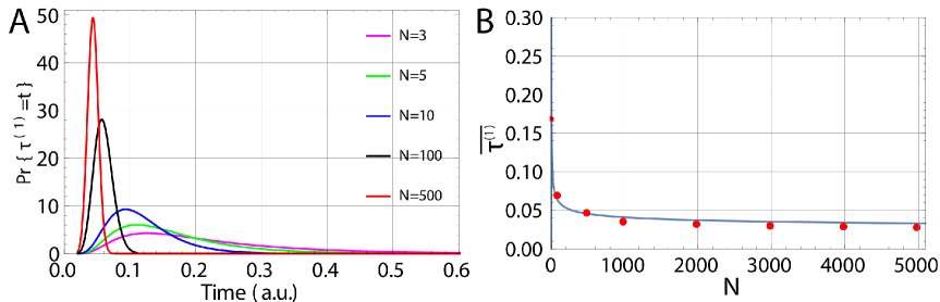
Figure 3: A. Plot of $\Pr\{\tau^{(1)}=t\}$ (escape from an interval) for $N=3,5,10,100$, and $500$ with $n_{0}=100$ terms in the series of (17). B. Decay of the expected arrival time of the fastest particle vs $N$ (red points). The plot of the asymptotic formula (65) is (blue) with parameter $\frac{0.282}{\log{N}}$.

The first line of (57) gives the approximation

$$\displaystyle\int\limits\limits_{0}^{a}\frac{1}{\sqrt{4\pi t}}\left[\exp\left\{-\frac{(x+y)^{2}}{4t}\right\}-\exp\left\{-\frac{(x-y)^{2}}{4t}\right\}\right]\,dx=\frac{1}{\sqrt{\pi}}\int\limits\limits_{(y-a)/2\sqrt{t}}^{y/2\sqrt{t}}e^{-u^{2}}\,du$$

$$\displaystyle\sim 1-\max\frac{2\sqrt{t}}{\sqrt{\pi}}\left[\frac{e^{-y^{2}/4t}}{y},\frac{e^{-(a-y)^{2}/4t}}{a-y}\right]\quad\mbox{as}\ t\to 0,$$ (59)

where the maximum occurs at $\min[y,a-y]$ for $0<y<a$ (the shortest ray from $y$ to the boundary). Starting at $x=a/2$, this gives

$$\Pr\{t_{1}>t\}= \displaystyle\int\limits\limits_{0}^{a}\frac{1}{\sqrt{4\pi t}}\left[\exp\left\{-\frac{(x-a/2)^{2}}{4t}\right\}-\exp\left\{-\frac{(x+a/2)^{2}}{4t}\right\}\right]\,dx\quad\mbox{as}\ t\to 0,$$

so changing $x+a/2=z\sqrt{4t}$ in the first integral and $x-a/2=z\sqrt{4t}$ in the second, we get

$$\frac{1}{\sqrt{\pi}}\int\limits\limits_{-a/4\sqrt{t}}^{a/4\sqrt{t}}e^{-z^{2}}\,dz-\frac{1}{\sqrt{\pi}}\int\limits\limits_{a/4\sqrt{t}}^{3a/4\sqrt{t}}e^{-z^{2}}\,dz\approx \,1-\frac{4\sqrt{t}e^{-a^{2}/16t}}{a\sqrt{\pi}}-\frac{2\sqrt{t}e^{-a^{2}/16t}}{a\sqrt{\pi}}-\frac{4\sqrt{t}e^{-9a^{2}/16t}}{6a\sqrt{\pi}}$$

$$= \,1-\frac{6\sqrt{t}e^{-a^{2}/16t}}{a\sqrt{\pi}}-\frac{2\sqrt{t}e^{-9a^{2}/16t}}{3a\sqrt{\pi}}.$$ (60)

The second integral in the second line of (57) is

$$I_{3/2}=-\displaystyle\int\limits\limits_{0}^{a}\frac{1}{\sqrt{4\pi t}}\left[\exp\left\{-\frac{(x-3a/2)^{2}}{4t}\right\}\right]\,dx.$$ (61)

Set $x-3a/2=-z\sqrt{4t}$, then (61) becomes

$$I_{3/2}=-\displaystyle\frac{1}{\sqrt{\pi}}\int\limits\limits_{a/4\sqrt{t}}^{3a/4\sqrt{t}}\exp\left\{-z^{2}\right\}\,dz=-\displaystyle\frac{1}{\sqrt{\pi}}\int\limits\limits_{a/4\sqrt{t}}^{\infty}\exp\left\{-z^{2}\right\}\,dz+\displaystyle\frac{1}{\sqrt{\pi}}\int\limits\limits_{3a/4\sqrt{t}}^{\infty}\exp\left\{-z^{2}\right\}\,dz.$$

Thus the second line of (57) is

$$- \displaystyle\int\limits\limits_{0}^{a}\frac{1}{\sqrt{4\pi t}}\left[\exp\left\{-\frac{(x-3a/2)^{2}}{4t}\right\}-\exp\left\{-\frac{(x-5a/2)^{2}}{4t}\right\}\right]\,dx$$

$$\approx -\frac{2\sqrt{t}}{a\sqrt{\pi}}e^{-a^{2}/16t}+\frac{2\sqrt{t}}{5a\sqrt{\pi}}e^{-25a^{2}/16t},$$ (62)

and in the third line of (57), we get

$$\displaystyle\int\limits\limits_{0}^{a}\frac{1}{\sqrt{4\pi t}}\left[\exp\left\{-\frac{(x+3a/2)^{2}}{4t}\right\}-\exp\left\{-\frac{(x+5a/2)^{2}}{4t}\right\}\right]\,dx$$

$$\approx \frac{2\sqrt{t}}{3a\sqrt{\pi}}e^{-9a^{2}/16t}-\frac{2\sqrt{t}}{5a\sqrt{\pi}}e^{-49a^{2}/16t},$$ (63)

hence

$$\int\limits\limits_{0}^{\infty}\left[\Pr\{t_{1}>t\}\right]^{N}dt\approx\int\limits\limits_{0}^{\infty}\exp\left\{N\ln\left(1-\frac{8\sqrt{t}}{a\sqrt{\pi}}e^{-a^{2}/16t}\right)\right\}dt$$ (64)

and the expected time of the fastest particle that starts at the center of the interval is (48) with $a$ replaced by $a/2$ and $N$ replaced by $2N$. That is,

$$\bar{\tau}^{1}\approx\frac{a^{2}}{16D\ln\frac{2N}{\sqrt{\pi}}}\quad\mbox{for}\ N\gg 1.$$ (65)

Figure 3A shows plot of the pdf analytical approximation of shortest arrival time (17) with $n_{0}=100$ terms, $D=1$ and $L=1$ for $N=4,6$, and $10$. As the number of particles increases, the mean first arrival time decreases (Fig.3B) and according to equation (65), the asymptotic behavior is given by $C/\log N,$ where $C$ is a constant. We show below the pdf of the fastest Brownian particle.

6 The shortest NEP from a bounded domain in $\hbox{\bb R}^{2,3}$

To generalize the previous result to the case of $N$ i.i.d. Brownian particles in a bounded domain $\Omega\subset\hbox{\bb R}^{2,3}$, we assume that the particles are initially injected at a point $\mbox{\boldmath$y$}\in\Omega$ and they can escape through a single small absorbing window $\partial\Omega_{a}$ in the boundary $\partial\Omega$ of the domain. The pdf of the fist passage time to $\partial\Omega_{a}$ is given by (8).

6.1 Asymptotics in dimension 3

To determine the short-time asymptotics of the pdf, we use the Laplace transform of the IBVP (3) and solve the resulting elliptic mixed Neumann-Dirichlet BVP [22]. The Dirichlet part of the boundary consists of $N$ well-separated small absorbing windows, $\partial\Omega_{a}=\bigcup_{j=1}^{N}\partial\Omega_{j}$ and the reflecting (Neumann) part is $\partial\Omega_{r}=\partial\Omega-\partial\Omega_{a}$, so that the IBVP (3) has the form

$$\frac{\partial p(\mbox{\boldmath$x$},t\,|\,\mbox{\boldmath$y$})}{\partial t}= D\Delta p(\mbox{\boldmath$x$},t\,|\,\mbox{\boldmath$y$})$$ (66)

$$p(\mbox{\boldmath$x$},0\,|\,\mbox{\boldmath$y$})= \delta(\mbox{\boldmath$x$}-\mbox{\boldmath$y$})\;\hbox{ for }\;\mbox{\boldmath$x$},\mbox{\boldmath$y$}\in\Omega$$

$$\displaystyle\frac{\partial p(\mbox{\boldmath$x$},t\,|\,\mbox{\boldmath$y$})}{\partial\mbox{\boldmath$n$}}= 0\;\;\hbox{for}\;\;\mbox{\boldmath$x$}\,\in\,\partial\Omega_{r}$$

$$p(\mbox{\boldmath$x$},t\,|\,\mbox{\boldmath$y$})= 0\;\;\hbox{ for }\;\;t>0,\ \mbox{\boldmath$x$}\,\in\,\partial\Omega_{a}.$$

We consider the case $N=1$. The Laplace transform of (3),

$$\hat{p}(\mbox{\boldmath$x$},q\,|\,\mbox{\boldmath$y$})=\int\limits_{0}^{\infty}p(\mbox{\boldmath$x$},t\,|\,\mbox{\boldmath$y$})e^{-pt}\,dt,$$ (67)

gives the BVP

$$-\delta(\mbox{\boldmath$x$}-\mbox{\boldmath$y$})+q\hat{p}(\mbox{\boldmath$x$},q\,|\,\mbox{\boldmath$y$})= D\Delta\hat{p}(\mbox{\boldmath$x$},q\,|\,\mbox{\boldmath$y$})\hskip 5.0pt\mbox{for}\ \mbox{\boldmath$x$},\mbox{\boldmath$y$}\in\Omega$$

$$\displaystyle\frac{\partial\hat{p}(\mbox{\boldmath$x$},q\,|\,\mbox{\boldmath$y$})}{\partial\mbox{\boldmath$n$}}= 0\;\;\hbox{for}\;\;\mbox{\boldmath$x$}\,\in\,\partial\Omega_{r}$$

$$\hat{p}(\mbox{\boldmath$x$},q\,|\,\mbox{\boldmath$y$})= 0\;\;\hbox{ for }\;\;\mbox{\boldmath$x$}\,\in\,\partial\Omega_{a}.$$

Green’s function for the Neumann problem in $\Omega$ is the solution of

$$-\Delta_{\mbox{\boldmath$x$}}\hat{G}(\mbox{\boldmath$x$},q\,|\,\mbox{\boldmath$y$})+q\hat{G}(\mbox{\boldmath$x$},q\,|\,\mbox{\boldmath$y$})= \delta(\mbox{\boldmath$x$}-\mbox{\boldmath$y$})\hskip 5.0pt\hbox{ for }\mbox{\boldmath$x$},\mbox{\boldmath$y$}\in\Omega,$$ (68)

$$\frac{\partial\hat{G}_{q}(\mbox{\boldmath$x$},q\,|\,\mbox{\boldmath$y$})}{\partial n_{\mbox{\boldmath$x$}}}= 0\hskip 5.0pt\hbox{ for }\mbox{\boldmath$x$},\mbox{\boldmath$y$}\in\partial\Omega.$$

The asymptotic solution of (68) in $\hbox{\bb R}^{3}$ is given by

$$\hat{G}(\mbox{\boldmath$x$},q\,|\,\mbox{\boldmath$y$})=\frac{e^{-\sqrt{q}|\mbox{\boldmath$x$}-\mbox{\boldmath$y$}|}}{4\pi||\mbox{\boldmath$x$}-\mbox{\boldmath$y$}||}+R_{q}(\mbox{\boldmath$x$},\mbox{\boldmath$y$}),$$ (69)

where $R_{q}(\mbox{\boldmath$x$},\mbox{\boldmath$y$})$ is more regular than the first term. When $x$ (or $y$) is on the boundary,

$$\hat{G}(\mbox{\boldmath$x$},q\,|\,\mbox{\boldmath$y$})=e^{-\sqrt{q}|\mbox{\boldmath$x$}-\mbox{\boldmath$y$}|}\left(\frac{1}{2\pi||\mbox{\boldmath$x$}-\mbox{\boldmath$y$}||}+\frac{H(\mbox{\boldmath$x$})}{2\pi}\log|\mbox{\boldmath$x$}-\mbox{\boldmath$y$}|+R(\mbox{\boldmath$x$},\mbox{\boldmath$y$})\right),$$ (70)

where $R(\mbox{\boldmath$x$},\mbox{\boldmath$y$})$ is more regular than the logarithmic term and $H(\mbox{\boldmath$x$})$ is a geometric factor [22]. Using Green’ identity, we obtain that

$$\int\limits\limits_{\Omega}\left[\hat{p}(\mbox{\boldmath$x$},q\,|\,\mbox{\boldmath$y$})\Delta_{\mbox{\boldmath$x$}}\hat{G}(\mbox{\boldmath$x$},q\,|\,\mbox{\boldmath$y$})-\Delta_{\mbox{\boldmath$x$}}\hat{p}(\mbox{\boldmath$x$},q\,|\,\mbox{\boldmath$y$})\hat{G}(\mbox{\boldmath$x$},q\,|\,\mbox{\boldmath$y$})\right]\,d\mbox{\boldmath$y$}$$

$$= \int\limits\limits_{\partial\Omega}\left[\hat{p}(\mbox{\boldmath$x$},q\,|\,\mbox{\boldmath$y$})\frac{\partial\hat{G}(\mbox{\boldmath$x$},q\,|\,\mbox{\boldmath$y$})}{\partial n_{\mbox{\boldmath$x$}}}-\frac{\partial\hat{p}(\mbox{\boldmath$x$},q\,|\,\mbox{\boldmath$y$})}{\partial n_{\mbox{\boldmath$x$}}}\hat{G}(\mbox{\boldmath$x$},q\,|\,\mbox{\boldmath$y$})\right]\,dS_{\mbox{\boldmath$y$}},$$

hence

$$\hat{p}(\mbox{\boldmath$x$},q\,|\,\mbox{\boldmath$y$})=\hat{G}(\mbox{\boldmath$x$},q\,|\,\mbox{\boldmath$y$})-\int\limits\limits_{\partial\Omega_{a}}\frac{\partial\hat{p}(\mbox{\boldmath$x$},q\,|\,\mbox{\boldmath$y$}^{\prime})}{\partial n_{\mbox{\boldmath$x$}}}\hat{G}(\mbox{\boldmath$x$},q\,|\,\mbox{\boldmath$y$}^{\prime})\,dS_{\mbox{\boldmath$y$}^{\prime}}.$$ (71)

If the absorbing window $\partial\Omega_{a}$ is centered at $\mbox{\boldmath$x$}=\mbox{\boldmath$A$}$, then, for $\mbox{\boldmath$x$}\in\partial\Omega_{a}$,

$$0=\hat{G}(\mbox{\boldmath$A$},q\,|\,\mbox{\boldmath$y$})-\int\limits\limits_{\partial\Omega_{a}}\frac{\partial\hat{p}(\mbox{\boldmath$A$},q\,|\,\mbox{\boldmath$y$}^{\prime})}{\partial n_{\mbox{\boldmath$x$}}}\hat{G}(\mbox{\boldmath$A$},q\,|\,\mbox{\boldmath$y$}^{\prime})\,dS_{\mbox{\boldmath$y$}^{\prime}}.$$ (72)

This is a Helmoltz equation and the solution is given by [22]

$$\hat{p}(\mbox{\boldmath$A$},q\,|\,\mbox{\boldmath$y$})=\frac{C}{\sqrt{a^{2}-r^{2}}},$$ (73)

where $r=|\mbox{\boldmath$A$}-\mbox{\boldmath$y$}|$. Thus, $C$ is computed from

$$0=G_{q}(\mbox{\boldmath$A$},\mbox{\boldmath$y$})-\int\limits_{\partial\Omega_{a}}\frac{\partial\hat{p}(\mbox{\boldmath$A$},q,\mbox{\boldmath$y$}\,|\,\mbox{\boldmath$y$})}{\partial n_{\mbox{\boldmath$x$}}}G_{q}(\mbox{\boldmath$A$},\mbox{\boldmath$y$})dS_{\mbox{\boldmath$y$}}$$ (74)

and to leading order,

$$G_{q}(\mbox{\boldmath$A$},\mbox{\boldmath$y$})=\int\limits_{\partial\Omega_{a}}\frac{Ce^{-\sqrt{q}|\mbox{\boldmath$y$}-\mbox{\boldmath$A$}|}}{\sqrt{a^{2}-r^{2}}}\left(\frac{1}{2\pi||\mbox{\boldmath$y$}-\mbox{\boldmath$A$}||}+\frac{H(\mbox{\boldmath$x$})}{2\pi}\log|\mbox{\boldmath$y$}-\mbox{\boldmath$A$}|+R(\mbox{\boldmath$y$},\mbox{\boldmath$A$})\right)dS_{\mbox{\boldmath$y$}}.$$ (75)

If $\partial\Omega_{a}$ is a disk of radius $a$, then

$$G_{q}(\mbox{\boldmath$A$},\mbox{\boldmath$y$})\approx C\int\limits_{\partial\Omega_{a}}\frac{e^{-\sqrt{q}r}}{\sqrt{a^{2}-r^{2}}}\frac{1}{2\pi r}2\pi rdr=\frac{\pi}{2}\left(I_{0}(\sqrt{q}a)-L_{0}(\sqrt{q}a)\right)C,$$ (76)

where $I_{0}$ is the modified Bessel function of the first kind and $L_{0}$ the Struve function. Thus,

$$\hat{p}(\mbox{\boldmath$x$},q\,|\,\mbox{\boldmath$y$})=G_{q}(\mbox{\boldmath$x$},\mbox{\boldmath$y$})-G_{q}(\mbox{\boldmath$A$},\mbox{\boldmath$y$})\frac{2}{\pi\left(I_{0}(\sqrt{q}a)-L_{0}(\sqrt{q}a)\right)}\int\limits_{\partial\Omega_{a}}\frac{G_{q}(\mbox{\boldmath$x$},\mbox{\boldmath$y$})dS_{\mbox{\boldmath$y$}}}{\sqrt{a^{2}-r^{2}}}.$$ (77)

For $|\mbox{\boldmath$A$}-\mbox{\boldmath$x$}|\gg a$ and q large, $I_{0}(\sqrt{q}a)-L_{0}(\sqrt{q}a)\approx\frac{2}{\pi\sqrt{q}a}$

$$\hat{p}(\mbox{\boldmath$x$},q\,|\,\mbox{\boldmath$y$})\approx G_{q}(\mbox{\boldmath$x$},\mbox{\boldmath$y$})-G_{q}(\mbox{\boldmath$A$},\mbox{\boldmath$y$})G_{q}(\mbox{\boldmath$A$},\mbox{\boldmath$x$})\frac{2}{\pi(I_{0}(\sqrt{q}a)-L_{0}(\sqrt{q}a))}\int\limits_{\partial\Omega_{a}}\frac{dS_{\mbox{\boldmath$y$}}}{\sqrt{a^{2}-r^{2}}},$$

hence, for a small circular window of radius $a$

$$\hat{p}(\mbox{\boldmath$x$},q\,|\,\mbox{\boldmath$y$})\approx G_{q}(\mbox{\boldmath$x$},\mbox{\boldmath$y$})-2\pi\sqrt{q}a^{2}G_{q}(\mbox{\boldmath$A$},\mbox{\boldmath$y$})G_{q}(\mbox{\boldmath$A$},\mbox{\boldmath$x$})+o(a^{2})\quad\mbox{for}\ a\ll 1.$$ (78)

To leading order in small $t$ and $\mbox{\boldmath$x$},\mbox{\boldmath$y$}\in\Omega$, we obtain for the first term using the leading order term in expression 69,

$${\mathcal{L}}^{-1}(G_{q}(\mbox{\boldmath$x$},\mbox{\boldmath$y$}))\approx\displaystyle\frac{1}{{(4\pi t)^{3/2}}}e^{\displaystyle-\frac{|\mbox{\boldmath$x$}-\mbox{\boldmath$y$}|^{2}}{4t}}.$$ (79)

We will now use the inverse Laplace transform [23][p.1026; 29.3.87]

$${\mathcal{L}}^{-1}(\sqrt{q}\frac{e^{-\sqrt{q}|\mbox{\boldmath$x$}-\mbox{\boldmath$y$}|}}{|\mbox{\boldmath$x$}-\mbox{\boldmath$y$}|})=\displaystyle\frac{1}{4\sqrt{\pi t^{3}}}e^{\displaystyle-\frac{|\mbox{\boldmath$x$}-\mbox{\boldmath$y$}|^{2}}{4t}}H_{2}(\frac{|\mbox{\boldmath$x$}-\mbox{\boldmath$y$}|}{2\sqrt{t}}),$$ (80)

where $H_{2}(x)=4x^{2}-2$ is the Hermite polynomial of degree 2. With $\mbox{\boldmath$A$}\in\partial\Omega$, the image charge (for the Dirichlet boundary) leads to a factor $1/2$ and we write

$$G_{q}(\mbox{\boldmath$A$},\mbox{\boldmath$y$})G_{q}(\mbox{\boldmath$A$},\mbox{\boldmath$x$})2\pi\sqrt{q}a^{2}=\sqrt{q}a^{2}\frac{e^{\displaystyle-\sqrt{q}(|\mbox{\boldmath$A$}-\mbox{\boldmath$y$}|+|\mbox{\boldmath$A$}-\mbox{\boldmath$x$}|)}}{2\pi|\mbox{\boldmath$A$}-\mbox{\boldmath$y$}||\mbox{\boldmath$A$}-\mbox{\boldmath$x$}|}$$ (81)

and

$${\mathcal{L}}^{-1}(G_{q}(\mbox{\boldmath$A$},\mbox{\boldmath$y$})G_{q}(\mbox{\boldmath$A$},\mbox{\boldmath$x$})\sqrt{q}a^{2})=\frac{a^{2}}{(4\pi t)^{3}}\frac{e^{-\displaystyle\frac{(|\mbox{\boldmath$A$}-\mbox{\boldmath$y$}|+|\mbox{\boldmath$A$}-\mbox{\boldmath$x$}|)^{2}}{4t}}}{{|\mbox{\boldmath$A$}-\mbox{\boldmath$y$}||\mbox{\boldmath$A$}-\mbox{\boldmath$x$}|}}H_{2}(\frac{|\mbox{\boldmath$A$}-\mbox{\boldmath$y$}|+|\mbox{\boldmath$A$}-\mbox{\boldmath$x$}|}{2\sqrt{t}}).$$ (82)

Finally,

$$\displaystyle{\mathcal{L}}^{-1}(\hat{p}(\mbox{\boldmath$x$},q\,|\,\mbox{\boldmath$y$}))=\frac{1}{\sqrt{(4\pi t)^{3}}}\left(e^{\displaystyle-\frac{|\mbox{\boldmath$x$}-\mbox{\boldmath$y$}|^{2}}{4t}}-\frac{a^{2}}{{|\mbox{\boldmath$A$}-\mbox{\boldmath$y$}||\mbox{\boldmath$A$}-\mbox{\boldmath$x$}|}}e^{-\displaystyle\frac{(|\mbox{\boldmath$A$}-\mbox{\boldmath$y$}|+|\mbox{\boldmath$A$}-\mbox{\boldmath$x$}|)^{2}}{4t}}H_{2}(\frac{|\mbox{\boldmath$A$}-\mbox{\boldmath$y$}|+|\mbox{\boldmath$A$}-\mbox{\boldmath$x$}|}{2\sqrt{t}})\right).$$ (83)

The short-time asymptotics of the survival probability with $\delta=|\mbox{\boldmath$A$}-\mbox{\boldmath$y$}|$,

$$S(t) \approx \displaystyle\int\limits_{\Omega}p_{t}(\mbox{\boldmath$x$},\mbox{\boldmath$y$})d\mbox{\boldmath$x$}$$

$$= \frac{1}{\sqrt{(4\pi t)^{3}}}\int\limits_{\Omega}\left(e^{-\displaystyle\frac{|\mbox{\boldmath$x$}-\mbox{\boldmath$y$}|^{2}}{4t}}-\frac{a^{2}}{{|\mbox{\boldmath$A$}-\mbox{\boldmath$y$}||\mbox{\boldmath$A$}-\mbox{\boldmath$x$}|}}e^{-\displaystyle\frac{(|\mbox{\boldmath$A$}-\mbox{\boldmath$y$}|+|\mbox{\boldmath$A$}-\mbox{\boldmath$x$}|)^{2}}{4t}}H_{2}(\frac{|\mbox{\boldmath$A$}-\mbox{\boldmath$y$}|+|\mbox{\boldmath$A$}-\mbox{\boldmath$x$}|}{2\sqrt{t}})\right)d\mbox{\boldmath$x$}$$

$$= \displaystyle I_{1}(t)-I_{2}(t)-I_{3}(t)-I_{4}(t),$$ (85)

where for small t,

$$H_{2}(\frac{|\mbox{\boldmath$A$}-\mbox{\boldmath$y$}|+|\mbox{\boldmath$A$}-\mbox{\boldmath$x$}|}{2\sqrt{t}})\approx\frac{(|\mbox{\boldmath$A$}-\mbox{\boldmath$y$}|+|\mbox{\boldmath$A$}-\mbox{\boldmath$x$}|)^{2}}{t},$$ (86)

and

$$I_{1}(t) = \displaystyle\frac{1}{\sqrt{(4\pi t)^{3}}}\int\limits_{\Omega}e^{-\displaystyle\frac{|\mbox{\boldmath$x$}-\mbox{\boldmath$y$}|^{2}}{4t}}d\mbox{\boldmath$x$}$$ (87)

$$I_{2}(t) = \frac{1}{\sqrt{(4\pi t)^{3}}}\frac{a^{2}\delta}{t}\int\limits_{\Omega}\frac{1}{{|\mbox{\boldmath$A$}-\mbox{\boldmath$x$}|}}e^{-\displaystyle\frac{(\delta+|\mbox{\boldmath$A$}-\mbox{\boldmath$x$}|)^{2}}{4t}}d\mbox{\boldmath$x$}$$ (88)

$$I_{3}(t) = \frac{1}{\sqrt{(4\pi t)^{3}}}\frac{2a^{2}}{t}\int\limits_{\Omega}e^{-\displaystyle\frac{(\delta+|\mbox{\boldmath$A$}-\mbox{\boldmath$x$}|)^{2}}{4t}}d\mbox{\boldmath$x$}.$$ (89)

$$I_{4}(t) = \frac{1}{\sqrt{(4\pi t)^{3}}}\frac{a^{2}}{\delta t}\int\limits_{\Omega}|\mbox{\boldmath$A$}-\mbox{\boldmath$x$}|e^{-\displaystyle\frac{(\delta+|\mbox{\boldmath$A$}-\mbox{\boldmath$x$}|)^{2}}{4t}}d\mbox{\boldmath$x$}.$$ (90)

Each integral is evaluated in the short-time limit.

$$I_{1}(t) = \displaystyle\frac{1}{\sqrt{(4\pi t)^{3}}}\int\limits_{\Omega}e^{-\displaystyle\frac{|\mbox{\boldmath$x$}-\mbox{\boldmath$y$}|^{2}}{4t}}d\mbox{\boldmath$x$}\approx 1-\frac{2}{\sqrt{\pi}}\int\limits\limits_{R_{a}/\sqrt{4t}}^{\infty}e^{-u^{2}}\,du$$ (91)

$$\approx 1-\sqrt{4t}\frac{e^{-\left(R_{a}/\sqrt{4t}\right)^{2}}}{R_{a}\sqrt{\pi}}\left(1+O\left(\left(R_{a}/\sqrt{4t}\right)^{2}\right)\right),$$ (92)

where $R_{a}$ is the radius of the maximal ball inscribed in $\Omega$. The integral $I_{2}$ is evaluated by the change of variables $\mbox{\boldmath$z$}=\mbox{\boldmath$x$}-\mbox{\boldmath$A$}$ and then $\eta=(\delta+r)/\sqrt{4t}$, where $r=|\mbox{\boldmath$z$}|$ (recall that $A$ is in $\Omega_{a}$),

$$I_{2}(t) = \frac{1}{\sqrt{(4\pi t)^{3}}}\frac{a^{2}\delta}{t}\int\limits_{\Omega}\frac{1}{{|\mbox{\boldmath$A$}-\mbox{\boldmath$x$}|}}e^{-\displaystyle\frac{(\delta+|\mbox{\boldmath$A$}-\mbox{\boldmath$x$}|)^{2}}{4t}}d\mbox{\boldmath$x$}$$ (93)

$$= \frac{1}{\sqrt{(4\pi t)^{3}}}\frac{a^{2}\delta}{t}\int\limits_{\Omega+\mbox{\boldmath$A$}}\frac{1}{{|\mbox{\boldmath$z$}|}}e^{-\displaystyle\frac{(\delta+|\mbox{\boldmath$z$}|)^{2}}{4t}}2\pi|\mbox{\boldmath$z$}|^{2}d|\mbox{\boldmath$z$}|$$ (94)

$$\approx \frac{2\pi}{\sqrt{(4\pi t)^{3}}}\frac{a^{2}\delta}{t}\int\limits_{\frac{\delta}{\sqrt{4t}}}^{\frac{\delta+R}{\sqrt{4t}}}e^{-\displaystyle\eta^{2}}(\sqrt{4t}\eta-\delta)\sqrt{4t}d\eta,$$ (95)

where $R$ is the radius of the largest half-ball centered at $\mbox{\boldmath$A$}\in\Omega_{a}$ and inscribed in $\Omega$. For short time,

$$\int\limits_{\frac{\delta}{\sqrt{4t}}}^{\frac{\delta+R}{\sqrt{4t}}}e^{-\displaystyle\eta^{2}}d\eta \approx \frac{1}{2}\left\{\frac{\sqrt{4t}}{\delta}e^{-\displaystyle\left(\frac{\delta}{\sqrt{4t}}\right)^{2}}\right\}\left(1-\frac{4t}{2\delta^{2}}+12\frac{t^{2}}{\delta^{4}}\right)$$ (96)

$$\int\limits_{\frac{\delta}{\sqrt{4t}}}^{\frac{\delta+R}{\sqrt{4t}}}\eta e^{-\displaystyle\eta^{2}}d\eta = \frac{1}{2}\left(e^{-\displaystyle\left(\frac{\delta}{\sqrt{4t}}\right)^{2}}-e^{-\displaystyle\left(\frac{\delta+R}{\sqrt{4t}}\right)^{2}}\right)\approx\frac{1}{2}e^{-\displaystyle\left(\frac{\delta}{\sqrt{4t}}\right)^{2}}.$$ (97)

Therefore,

$$I_{2}(t) \approx \frac{1}{\sqrt{(4\pi t)^{3}}}\frac{2\pi a^{2}\delta}{t}\left(2te^{-\displaystyle\left(\frac{\delta}{\sqrt{4t}}\right)^{2}}-\delta\sqrt{4t}\frac{1}{2}\left(\frac{\sqrt{4t}}{\delta}e^{-\displaystyle(\frac{\delta}{\sqrt{4t}})^{2}}\right)(1-\frac{4t}{2\delta^{2}}+12\frac{t^{2}}{\delta^{4}})\right)$$ (98)

$$\approx \frac{4a^{2}}{\delta\sqrt{\pi}}\frac{1}{\sqrt{t}}(1-\frac{6t}{\delta^{2}})e^{-\displaystyle\left(\frac{\delta}{\sqrt{4t}}\right)^{2}}.$$ (99)

Now,

$$I_{3}(t) = \frac{1}{\sqrt{(4\pi t)^{3}}}\frac{2a^{2}}{t}\int\limits_{\Omega}e^{-\displaystyle\frac{(\delta+|\mbox{\boldmath$A$}-\mbox{\boldmath$x$}|)^{2}}{4t}}d\mbox{\boldmath$x$}$$ (100)

$$= \frac{2\pi}{\sqrt{(4\pi t)^{3}}}\frac{2a^{2}}{t}\int\limits_{\frac{\delta}{\sqrt{4t}}}^{\frac{\delta+R}{\sqrt{4t}}}e^{-\displaystyle\eta^{2}}(\sqrt{4t}\eta-\delta)^{2}\sqrt{4t}d\eta$$ (101)

$$= \frac{2\pi}{\sqrt{(4\pi t)^{3}}}\frac{2a^{2}}{t}\int\limits_{\frac{\delta}{\sqrt{4t}}}^{\frac{\delta+R}{\sqrt{4t}}}e^{-\displaystyle\eta^{2}}(4t\eta^{2}-2\sqrt{4t}\eta\delta+\delta^{2})\sqrt{4t}d\eta,$$ (102)

that we write as $I_{3}(t)=I^{(1)}_{3}(t)+I^{(2)}_{3}(t)+I^{(3)}_{3}(t)$. The approximation

$$\int\limits_{\frac{\delta}{\sqrt{4t}}}^{\frac{\delta+R}{\sqrt{4t}}}e^{-\displaystyle\eta^{2}}\eta^{2}d\eta\approx\frac{\delta}{2\sqrt{4t}}\,e^{-\displaystyle\left(\frac{\delta}{\sqrt{4t}}\right)^{2}}+\frac{1}{4}\left(\frac{\sqrt{4t}}{\delta}e^{-\displaystyle\left(\frac{\delta}{\sqrt{4t}}\right)^{2}}\right)\left(1-\frac{4t}{2\delta^{2}}+o(t)\right),$$ (103)

gives

$$I^{(1)}_{3}(t)= \frac{2\pi\delta}{\pi^{3/2}}\frac{a^{2}}{{t\sqrt{4t}}}e^{-\displaystyle\{\frac{\delta}{\sqrt{4t}}\}^{2}}+\frac{2a^{2}}{2t\pi^{3/2}}\frac{1}{{\delta^{2}}}\sqrt{4t}e^{-\displaystyle(\frac{\delta}{\sqrt{4t}})^{2}}\left(1-\frac{4t}{2\delta^{2}}\right)$$

$$I^{(2)}_{3}(t)= -\frac{4\pi a^{2}\delta}{t\sqrt{4t}\pi^{3/2}}e^{-\displaystyle(\frac{\delta}{\sqrt{4t}})^{2}}$$

$$I^{(3)}_{3}(t)= \frac{2\pi a^{2}\delta}{t\sqrt{4t}\pi^{3/2}}e^{-\displaystyle\left(\frac{\delta}{\sqrt{4t}}\right)^{2}}\left(1-\frac{4t}{2\delta^{2}}+o(t)\right).$$

Summing the three contributions, the leading order terms cancel and

$$I_{3}(t)=\frac{4a^{2}\sqrt{t}}{\pi^{1/2}\delta^{3}}e^{-\displaystyle\left(\frac{\delta}{\sqrt{4t}}\right)^{2}}.$$ (104)

To compute $I_{4}$, we decompose it into 4 pieces:

$$I_{4}(t) = \frac{1}{\sqrt{(4\pi t)^{3}}}\frac{a^{2}}{\delta t}\int\limits_{\Omega}|\mbox{\boldmath$A$}-\mbox{\boldmath$x$}|e^{-\displaystyle\frac{(\delta+|\mbox{\boldmath$A$}-\mbox{\boldmath$x$}|)^{2}}{4t}}d\mbox{\boldmath$x$}.$$ (105)

$$= \frac{2\pi}{\sqrt{(4\pi t)^{3}}}\frac{a^{2}}{\delta t}\int\limits_{\frac{\delta}{\sqrt{4t}}}^{\frac{\delta+R}{\sqrt{4t}}}e^{-\displaystyle\eta^{2}}(\sqrt{4t}\eta-\delta)^{3}\sqrt{4t}d\eta$$ (106)

$$= J_{1}(t)+J_{2}(t)+J_{3}(t)+J_{4}(t).$$ (107)

Direct computations give:

$$J_{1}(t)=\frac{2\pi(4t)^{2}}{\sqrt{(4\pi t)^{3}}}\frac{a^{2}}{\delta t}\int\limits_{\frac{\delta}{\sqrt{4t}}}^{\frac{\delta+R}{\sqrt{4t}}}e^{-\displaystyle\eta^{2}}\eta^{3}d\eta=\frac{4a^{2}\delta}{\sqrt{\pi}(4t)^{3/2}}(1+\frac{4t}{\delta^{2}})e^{-\displaystyle\left(\frac{\delta}{\sqrt{4t}}\right)^{2}},$$ (108)

where we used

$$\int\limits_{\frac{\delta}{\sqrt{4t}}}^{\frac{\delta+R}{\sqrt{4t}}}\eta^{3}e^{-\displaystyle\eta^{2}}d\eta \approx \left(1+\frac{\delta^{2}}{4t}\right)e^{-\displaystyle\left(\frac{\delta}{\sqrt{4t}}\right)^{2}}.$$ (109)

Next,

$$J_{2}(t)=-\frac{2\pi}{\sqrt{(\pi)^{3}}}\frac{a^{2}}{\delta t}\int\limits_{\frac{\delta}{\sqrt{4t}}}^{\frac{\delta+R}{\sqrt{4t}}}e^{-\displaystyle\eta^{2}}3\eta^{2}\delta d\eta=-\frac{12a^{2}\delta}{\sqrt{\pi}(4t)^{3/2}}\left(1+\frac{2t}{\delta^{2}}(1-\frac{2t}{\delta^{2}}+\frac{12t^{2}}{\delta^{4}}+o(t^{2}))\right)e^{-\displaystyle\left(\frac{\delta}{\sqrt{4t}}\right)^{2}},$$ (110)

where we have used

$$\int\limits_{\frac{\delta}{\sqrt{4t}}}^{\frac{\delta+R}{\sqrt{4t}}}\eta^{2}e^{-\displaystyle\eta^{2}}d\eta \approx \left(\frac{\delta}{2\sqrt{4t}}+\frac{\sqrt{4t}}{4\delta}\left(1-\frac{4t}{2\delta^{2}}+12\frac{t^{2}}{\delta^{4}}+o(t^{2})\right)\right)e^{-\displaystyle\left(\frac{\delta}{\sqrt{4t}}\right)^{2}}$$ (111)

Using relation 96,

$$J_{3}(t)=\frac{2\pi}{\sqrt{(4t\pi^{3})}}\frac{a^{2}}{\delta t}\int\limits_{\frac{\delta}{\sqrt{4t}}}^{\frac{\delta+R}{\sqrt{4t}}}e^{-\displaystyle\eta^{2}}3\eta\delta^{2}d\eta=\frac{12a^{2}\delta}{\sqrt{\pi}(4t)^{3/2}}e^{\displaystyle-\frac{\delta^{2}}{4t}}.$$ (112)

Finally,

$$J_{4}(t)=-\frac{2\pi}{4t\sqrt{(\pi)^{3}}}\frac{a^{2}}{\delta t}\int\limits_{\frac{\delta}{\sqrt{4t}}}^{\frac{\delta+R}{\sqrt{4t}}}e^{-\displaystyle\eta^{2}}\delta^{3}d\eta=\displaystyle-\frac{4a^{2}\delta}{(4t)^{3/2}\sqrt{\pi}}e^{\displaystyle-\frac{\delta^{2}}{4t}}\left(1-\frac{2t}{\delta^{2}}+\frac{12t^{2}}{\delta^{4}}+o(t^{2})\right).$$ (113)

Direct computations show that the terms in $t^{-3/2}$ and $t^{-1/2}$ cancels out in the computation of $I_{4}$ from the four terms $J_{1},..J_{4}$ and it remains only the term in $t^{1/2}$

$$I_{4}(t)=-\frac{9a^{2}}{\sqrt{\pi}\delta^{3}}t^{1/2}e^{\{-\delta^{2}/4t\}}.$$ (114)

Summing (91)-(104)-(105), we get

$$S(t) = \displaystyle\int\limits_{\Omega}p_{t}(\mbox{\boldmath$x$},\mbox{\boldmath$y$})d\mbox{\boldmath$x$}$$

$$= \displaystyle 1-\sqrt{4t}\,\frac{e^{-\left(R_{a}/\sqrt{4t}\right)^{2}}}{R_{a}\sqrt{\pi}}-\frac{a^{2}}{\delta\pi^{1/2}\sqrt{t}}\,e^{-\delta^{2}/4t}+o\left(t^{1/2}e^{-\displaystyle\left(\frac{\delta}{\sqrt{4t}}\right)^{2}}\right)$$

$$\approx \displaystyle 1-\frac{a^{2}}{\delta\pi^{1/2}\sqrt{t}}\,e^{-\delta^{2}/4t}.$$

It follows that in three dimensions, the expected shortest arrival time to a small circular window of radius $a$, the expected shortest time $\bar{\tau}^{3}$ is given by

$$\bar{\tau}^{3}=\int\limits\limits_{0}^{\infty}\left[\Pr\{t_{1}>t\}\right]^{N}dt \approx \int\limits\limits_{0}^{\infty}\exp N\log\left(1-\frac{a^{2}}{\delta\pi^{1/2}\sqrt{t}}\,e^{-\delta^{2}/4t}\right)dt$$

$$\approx \int\limits\limits_{0}^{\infty}\exp\left(-N\frac{4(a/\delta)}{\delta\pi^{3/2}\sqrt{t}}e^{-\delta^{2}/4t}\right)dt$$

$$\approx \delta^{2}\int\limits\limits_{0}^{\infty}\exp\left(-N^{\prime}\frac{1}{\sqrt{u}}e^{-1/4u}\right)du,$$

where $N^{\prime}=N\frac{4a^{2}}{\pi^{1/2}\delta^{2}}$ Using the method develop in section 4.1 with the change of variable,

$$w=w(t)=\frac{1}{\sqrt{t}}e^{-1/t},\quad w^{\prime}(t)=\frac{1}{\sqrt{t}}e^{-\frac{1}{t}}\left(-\frac{1}{2t}+\frac{1}{4t^{3/2}}\right).$$ (115)

We have with $w^{\prime}=4w(\log(w))^{3/2}$

$$\bar{\tau}^{3} \approx \delta^{2}\int\limits\limits_{0}^{\infty}\frac{\exp(-N^{\prime}w)}{4w(\log(w))^{3/2}}du$$

When the diffusion coefficient is $D$, the formula changes to

$$\bar{\tau}^{3}\approx\frac{\delta^{2}}{2D\sqrt{\log\left(\displaystyle N\frac{4a^{2}}{\pi^{1/2}\delta^{2}}\right)}}.$$ (116)

The next term in the expansion can be obtained by accounting for the logarithmic singularity in the expansion of Green’s function. When there are $p$ windows, whose distances from the initial position of the Brownian particle are $d_{k}=dist(P_{0},P_{k}$), formula (116) changes to

$$\bar{\tau}^{3}\approx\frac{\delta^{2}_{m}}{2D\sqrt{\log\left(\displaystyle N\frac{4a^{2}}{\pi^{1/2}\delta^{2}}\right)}},$$ (117)

where $\delta^{2}_{m}=\min(d_{1}^{2},..d_{p}^{2})$. The asymptotic formula (116) is compared with results of Brownian simulations and shows very good agreement (Fig. 4). When absorbing windows are ellipses, the Green’s function approach, based on Narrow Escape methodology, can be applied as well [17].

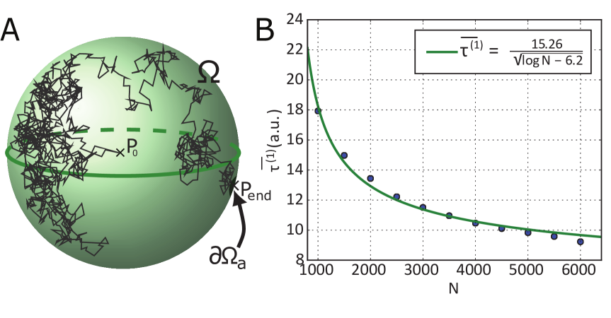
Figure 4: Extreme statistics of the narrow escape time through a small window in three dimensions. A. The geometry of the NEP for the fastest particle. In the simulation, the sphere has a radius $5\,\mu m$, the absorbing window $\partial{\mathcal{S}}_{a}$, has a radius $\varepsilon=0.1\mu m$ and the diffusion coefficient is $D=0.2\mu m^{2}s^{-1}$. The trajectory starts at point $P_{0}$ (cross), and ends at point $P_{end}$ . B. Plot of the MFPT of the fastest particle versus the number of particle $N$. We simulated 2000 runs. The asymptotic solution (red curve) is $A/\log(N+B)$.

6.2 Asymptotics in dimension 2

We consider the diffusion of $N$ Brownian i.i.d. particles in a two-dimensional domain $\Omega$ with a small absorbing arc $\partial\Omega_{a}$ of length $2\varepsilon$ on the otherwise reflecting boundary $\partial\Omega$. To compute the pdf of the shortest arrival time to the arc, we follow the steps of the analysis in dimension 3, presented in the previous subsection 6.1.

The Neumann-Green function (68) in two dimensions is the solution of the BVP

$$-\Delta_{\mbox{\boldmath$x$}}\hat{G}(\mbox{\boldmath$x$},q\,|\,\mbox{\boldmath$y$})+q\hat{G}(\mbox{\boldmath$x$},q\,|\,\mbox{\boldmath$y$})= \delta(\mbox{\boldmath$x$}-\mbox{\boldmath$y$})\hskip 5.0pt\hbox{ for }\mbox{\boldmath$x$},\mbox{\boldmath$y$}\in\Omega,$$ (118)

$$\frac{\partial\hat{G}_{q}(\mbox{\boldmath$x$},q\,|\,\mbox{\boldmath$y$})}{\partial n_{\mbox{\boldmath$x$}}}= 0\hskip 5.0pt\hbox{ for }\mbox{\boldmath$x$},\mbox{\boldmath$y$}\in\partial\Omega,$$ (119)

is given for $\mbox{\boldmath$x$},\mbox{\boldmath$y$}\in\partial\Omega$ by [24, p.51]

$$\hat{G}(\mbox{\boldmath$x$},q\,|\,\mbox{\boldmath$y$})=\frac{1}{\pi}K_{0}(\sqrt{q}|\mbox{\boldmath$x$}-\mbox{\boldmath$y$}|)+R(\mbox{\boldmath$x$},\mbox{\boldmath$y$}),$$ (120)

where $R(\mbox{\boldmath$x$},\mbox{\boldmath$y$})$ is its regular part. For a disk, the analytical expression is given by the series

$$R(\mbox{\boldmath$x$},\mbox{\boldmath$y$})=\frac{1}{\pi}\sum_{0}^{\infty}\sigma_{n}\cos(n(\psi-\psi_{0}))\frac{K^{\prime}_{n}(\sqrt{q})}{I^{\prime}_{n}(\sqrt{q})}I_{n}(r\sqrt{q})I_{n}(r_{0}\sqrt{q}),$$ (121)

where $\sigma_{0}=1,\sigma_{n}=2$ for $n\geq 2$ and $\mbox{\boldmath$x$}=re^{i\psi},\mbox{\boldmath$y$}=r_{0}e^{i\psi_{0}}$. The integral representation (71) of the solution is

$$\hat{p}(\mbox{\boldmath$x$},q\,|\,\mbox{\boldmath$y$})=\hat{G}(\mbox{\boldmath$x$},q\,|\,\mbox{\boldmath$y$})-\int\limits\limits_{\partial\Omega_{a}}\frac{\partial\hat{p}(\mbox{\boldmath$x$},q\,|\,\mbox{\boldmath$y$}^{\prime})}{\partial n_{\mbox{\boldmath$x$}}}\hat{G}(\mbox{\boldmath$x$},q\,|\,\mbox{\boldmath$y$}^{\prime})\,dS_{\mbox{\boldmath$y$}^{\prime}},$$ (122)

so choosing $\mbox{\boldmath$x$}\in\partial\Omega_{a}$,

$$0=\hat{G}(\mbox{\boldmath$x$},q\,|\,\mbox{\boldmath$y$})-\int\limits\limits_{\partial\Omega_{a}}\frac{\partial\hat{p}(\mbox{\boldmath$x$},q\,|\,\mbox{\boldmath$y$}^{\prime})}{\partial n_{\mbox{\boldmath$x$}}}\hat{G}(\mbox{\boldmath$x$},q\,|\,\mbox{\boldmath$y$}^{\prime})\,dS_{\mbox{\boldmath$y$}^{\prime}}.$$ (123)

This Helmholtz equation has the constant solution [17]

$$\frac{\partial\hat{p}(\mbox{\boldmath$x$},q\,|\,\mbox{\boldmath$y$}^{\prime})}{\partial n_{\mbox{\boldmath$x$}}}=C\hskip 5.0pt\mbox{for all}\ \mbox{\boldmath$x$}=\mbox{\boldmath$A$}\in\partial\Omega_{a}.$$ (124)

To leading order, we get

$$\hat{G}(\mbox{\boldmath$A$},q\,|\,\mbox{\boldmath$y$})=\frac{C}{\pi}\int\limits_{\partial\Omega_{a}}K_{0}(\sqrt{q}|\mbox{\boldmath$A$}-\mbox{\boldmath$y$}|)\,ds_{\mbox{\boldmath$y$}},$$ (125)

where $ds_{\mbox{\boldmath$y$}}$ is arclength element in $\partial\Omega_{a}$. When $|\mbox{\boldmath$x$}-\mbox{\boldmath$y$}|\leq 4\varepsilon$ and $\sqrt{q}\varepsilon\ll 1$ in the large $q$ expansion of Green’s function,

$$K_{0}(\sqrt{q}|\mbox{\boldmath$x$}-\mbox{\boldmath$y$}|)=-\log(\sqrt{q}|\mbox{\boldmath$x$}-\mbox{\boldmath$y$}|)+\log 2-\gamma_{0}+o(1),$$ (126)

we obtain

$$\hat{G}(\mbox{\boldmath$A$},q\,|\,\mbox{\boldmath$y$})=\frac{C}{\pi}\int\limits_{\partial\Omega_{a}}\left[\displaystyle-\log(\sqrt{q}|\mbox{\boldmath$A$}-\mbox{\boldmath$y$}|)+\log 2-\gamma_{0}+o(1)\right]\,ds_{\mbox{\boldmath$y$}};$$ (127)

that is,

$$\hat{G}(\mbox{\boldmath$A$},q\,|\,\mbox{\boldmath$y$})=\frac{2C}{\pi}\int\limits_{0}^{\varepsilon}\left[\displaystyle-\log(\sqrt{q}r)+\log 2-\gamma_{0}+o(1)\right]\,dr.$$ (128)

Therefore the leading order approximation of $C$ is

$$C=\frac{\pi\hat{G}(\mbox{\boldmath$A$},q\,|\,\mbox{\boldmath$y$})}{2\varepsilon\left[\displaystyle-\log(\sqrt{q}\varepsilon)+O(\varepsilon)\right]}.$$ (129)

Finally, (122) gives for $|\mbox{\boldmath$A$}-\mbox{\boldmath$x$}|\gg\varepsilon$

$$\hat{p}(\mbox{\boldmath$x$},q\,|\,\mbox{\boldmath$y$})\approx\hat{G}(\mbox{\boldmath$x$},q\,|\,\mbox{\boldmath$y$})+\frac{\pi\hat{G}(\mbox{\boldmath$A$},q\,|\,\mbox{\boldmath$y$})\hat{G}(\mbox{\boldmath$A$},q\,|\,\mbox{\boldmath$x$})}{\displaystyle\log(\sqrt{q}\varepsilon)+O(\varepsilon)}.$$ (130)

The inversion formula [23, p.1028] for $k>0$,

$${\mathcal{L}}^{-1}(K_{0}(k\sqrt{q})=\displaystyle\frac{1}{2t}e^{\displaystyle-\frac{k^{2}}{4t}},$$ (131)

gives

$${\mathcal{L}}^{-1}\hat{G}(\mbox{\boldmath$x$},q\,|\,\mbox{\boldmath$y$})=\displaystyle\frac{1}{4\pi t}e^{-\displaystyle\frac{|\mbox{\boldmath$x$}-\mbox{\boldmath$y$}|^{2}}{4t}}.$$ (132)

For an initial point far from the boundary layer near the window, the expansion [23, p.378]

$$K_{0}(z)=\displaystyle\sqrt{\frac{\pi}{2z}}e^{\displaystyle-z}\left(1+O\left(\frac{1}{z}\right)\right)\quad\mbox{for}\ z\gg 1,$$ (133)

gives in (120)

$$\hat{G}(\mbox{\boldmath$A$},q\,|\,\mbox{\boldmath$y$})\hat{G}(\mbox{\boldmath$A$},q\,|\,\mbox{\boldmath$x$})=\displaystyle\frac{1}{2\pi}\sqrt{\frac{1}{q{s_{1}s_{2}}}}e^{\displaystyle-\sqrt{q}(s_{1}+s_{2})}\left(1+O(q^{-1/2})\right),$$ (134)

where $s_{1}=|\mbox{\boldmath$A$}-\mbox{\boldmath$y$}|$ and $s_{2}=|\mbox{\boldmath$A$}-\mbox{\boldmath$x$}|$,

$$\frac{\pi\hat{G}(\mbox{\boldmath$A$},q\,|\,\mbox{\boldmath$y$})\hat{G}(\mbox{\boldmath$A$},q\,|\,\mbox{\boldmath$x$})}{\displaystyle-\log(\sqrt{q}\varepsilon)+O(\varepsilon)} = \displaystyle\frac{1}{-2\log(\sqrt{q}\varepsilon)}\sqrt{\frac{1}{q{s_{1}s_{2}}}}e^{\displaystyle-\sqrt{q}(s_{1}+s_{2})}\left(1+O(q^{-1/2})\right),$$

$$\approx \displaystyle\frac{1}{-2\log(\varepsilon)+O(1)}\sqrt{\frac{1}{q{s_{1}s_{2}}}}e^{\displaystyle-\sqrt{q}(s_{1}+s_{2})}\left(1+O(q^{-1/2})\right).$$

The inversion formula

$${\mathcal{L}}^{-1}\left(\frac{1}{\sqrt{q}}e^{\displaystyle-k\sqrt{q}}\right)=\displaystyle\frac{1}{\sqrt{\pi t}}e^{\displaystyle-\frac{k^{2}}{4t}}$$ (135)

gives

$$\frac{\pi{\mathcal{L}}^{-1}(\hat{G}(\mbox{\boldmath$A$},q\,|\,\mbox{\boldmath$y$})\hat{G}(\mbox{\boldmath$A$},q\,|\,\mbox{\boldmath$x$})}{\displaystyle-\log(\sqrt{q}\varepsilon)+O(\varepsilon)})=\frac{1}{-2\log(\varepsilon)+O(1)}\displaystyle\frac{1}{\sqrt{\pi ts_{1}s_{2}}}e^{\displaystyle-\frac{(s_{1}+s_{2})^{2}}{4t}}.$$ (136)

Hence, we obtain the short-time asymptotics of the survival probability

$$S(t) \approx \displaystyle\int\limits_{\Omega}p_{t}(\mbox{\boldmath$x$},\mbox{\boldmath$y$})\,d\mbox{\boldmath$x$}$$ (137)

$$= \displaystyle\frac{1}{4\pi t}\int\limits_{\Omega}e^{-\displaystyle\frac{|\mbox{\boldmath$x$}-\mbox{\boldmath$y$}|^{2}}{4t}}\,d\mbox{\boldmath$x$}$$ (139)

$$-\frac{1}{-2\log(\varepsilon)\sqrt{s_{2}}+O(1)}\frac{1}{\sqrt{\pi t}}\int\limits_{\Omega}\sqrt{\frac{1}{{|\mbox{\boldmath$A$}-\mbox{\boldmath$x$}|}}}\displaystyle e^{\displaystyle-\frac{(|\mbox{\boldmath$A$}-\mbox{\boldmath$x$}|+s_{2})^{2}}{4t}}d\mbox{\boldmath$x$}$$

$$= R_{1}(t)+R_{2}(t)$$ (140)

where

$$R_{1}(t) = \displaystyle\frac{1}{4\pi t}\int\limits_{\Omega}e^{-\displaystyle\frac{|\mbox{\boldmath$x$}-\mbox{\boldmath$y$}|^{2}}{4t}}d\mbox{\boldmath$x$}\approx 1-{e^{-\left(R_{a}/\sqrt{4t}\right)^{2}}},$$ (141)

and $R_{a}$ is the radius of the maximal disk inscribed in $\Omega$. The second term is

$$R_{2}(t) = -\frac{1}{-2\log(\varepsilon)\sqrt{s_{2}}+O(1)}\frac{1}{\sqrt{\pi t}}\int\limits_{\Omega}\sqrt{\frac{1}{{|\mbox{\boldmath$A$}-\mbox{\boldmath$x$}|}}}\displaystyle\,e^{\displaystyle-\frac{(|\mbox{\boldmath$A$}-\mbox{\boldmath$x$}|+s_{2})^{2}}{4t}}d\mbox{\boldmath$x$}$$ (142)

$$\approx -\frac{1}{-2\log(\varepsilon)\sqrt{s_{2}}+O(1)}\sqrt{\frac{\pi}{t}}\int\limits_{0}^{R_{a}}\displaystyle e^{\displaystyle-\frac{(r+s_{2})^{2}}{4t}}\sqrt{r}\,dr.$$

The small $t$ Laplace expansion and the two successive changes of variable $u=\frac{s_{2}}{2t}r$ and $v=u^{3/2}$ give

$$\int\limits_{0}^{R_{a}}\displaystyle e^{\displaystyle-\frac{(r+s_{2})^{2}}{4t}}\sqrt{r}dr\approx\frac{2}{3}\left(\frac{2t}{s_{2}}\right)^{3/2}e^{\displaystyle-\frac{s_{2}^{2}}{4t}}\int\limits_{0}^{\infty}e^{-v^{3/2}}dv.$$ (143)

Thus, with

$$I=\int\limits_{0}^{\infty}e^{-v^{2/3}}dv=\frac{3\sqrt{\pi}}{4},$$ (144)

we obtain

$$R_{2}(t)-\frac{1}{-2\log(\varepsilon)+O(1)}\frac{\sqrt{2}\pi t}{s_{2}^{2}}\displaystyle e^{\displaystyle-\frac{s_{2}^{2}}{4t}}.$$ (145)

We conclude therefore that the survival probability (137) is approximately

$$S(t) \approx 1-\frac{1}{2\log(\frac{1}{\varepsilon})}\frac{\sqrt{2}\pi t}{s_{2}^{2}}\displaystyle e^{\displaystyle-\frac{s_{2}^{2}}{4t}},$$ (146)

where the contribution of (141) is negligible. Thus the MFPT of the fastest particle is given by

$$\bar{\tau}^{2}=\int\limits\limits_{0}^{\infty}\left[\Pr\{t_{1}>t\}\right]^{N}dt \approx \int\limits\limits_{0}^{\infty}\exp\left\{N\log\left(1-\frac{1}{2\log(\frac{1}{\varepsilon})}\frac{\sqrt{2}\pi t}{s_{2}^{2}}\displaystyle e^{\displaystyle-\frac{s_{2}^{2}}{4t}}\right)\right\}dt$$

$$\approx \int\limits\limits_{0}^{\infty}\exp\left\{-N\frac{1}{2\log(\frac{1}{\varepsilon})}\frac{\sqrt{2}\pi t}{s_{2}^{2}}\displaystyle e^{\displaystyle-\frac{s_{2}^{2}}{4t}}\right\}dt.$$

The computation of the last integral follows the steps described in subsection 5. The change of variable $w=te^{\displaystyle-\frac{s_{2}^{2}}{4t}}$ leads to the asymptotic formula with diffusion coefficient $D$

$$\bar{\tau}^{2}\approx\displaystyle\frac{\displaystyle s_{2}^{2}}{\displaystyle 4D\log\left(\frac{\pi\sqrt{2}N}{8\log\left(\frac{1}{\varepsilon}\right)}\right)}.$$

where $s_{2}=|\mbox{\boldmath$x$}-\mbox{\boldmath$A$}|$ and $x$ is the position of injection $A$ the center of the absorbing window. This formula is compared with Brownian simulations in Fig. 5. However, the dependence on the window size is $\log(\frac{1}{\varepsilon})$.

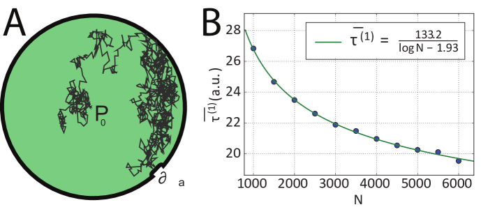
Figure 5: Escape through a narrow opening in a planar disk. A. The geometry of the NEP for the fastest particle. B. Plot of the MFPT of the fastest particle versus the number of particles $N$. The asymptotic solution (red curve) is of the form $\frac{\alpha}{\log(N)+\beta}$.

7 Application of extreme statistics in cell biology

7.1 The first arrival time of ions in a dendritic-spine geometry

The geometry of a dendritic spine (see Fig.6) is composed of a head with a small hole opening, connected to a cylindrical neck. Initially, all Brownian particles, which represent calcium ions that are uniformly distributed in the spine head at the time of their release. This geometry implies that the mean time $\tau$ to reach the base of the neck is the mean time $\tau^{1}$ to reach the small window for the first time plus the mean time $\tau^{2}$ spent in the spine neck, with no possible returns: we assume here that when a particle enters the neck cylinder, it cannot return to the head.

We compute now the distribution of the arrival time for the fastest and second fastest Brownian particle in a dendritic spine geometry. The pdf of a particle arriving at the base of the dendrite within the time $\tau=\tau^{1}+\tau^{2}$ is computed as follows, when the escape time form the head is Poissonian:

$$\Pr\{\tau=\tau_{1}+\tau_{2}=t\}=\int\limits_{0}^{t}\Pr\{\tau_{2}=t-s|\tau_{1}=s\}\Pr\{\tau_{1}=s\}ds.$$ (147)

The the Markovian property implies that

$$\Pr\{\tau_{1}+\tau_{2}=t\}=\int\limits_{0}^{t}\Pr\{\tau_{2}=t-s\}\Pr\{\tau_{1}=s\}ds.$$ (148)

Using the narrow escape theory [17], the distribution of arrival time of a Brownian particle at the entrance of the dendritic neck is Poissonian,

$$\Pr\{\tau^{1}=s\}=\gamma e^{-\gamma s},$$ (149)

where

$$\gamma^{-1}=\frac{|\Omega|}{4aD\left[1+\displaystyle\frac{L(\mbox{\boldmath$0$})+N(\mbox{\boldmath$0$})}{2\pi}\,a\log a+o(a\log a)\right]},$$

with $|\Omega|$ the volume of the spherical head, while $a$ is the radius of the cylindrical neck [17] and $L(0)$ and $N(0)$ are the principal mean curvature. After the first particles reaches the cylinder (spine neck), we approximate its Brownian motion in the cylindrical domain by one-dimensional motion (1D). By substituting $N=1$ for the first arriving particle, this is given by (16):

$$\Pr\{\tau_{2}=t-s\}=N_{R}\sum^{\infty}_{n=0}{(-1)^{n}}{\lambda_{n}}e^{-D\lambda^{2}_{n}(t-s)}.$$ (150)

Hence,

$$\Pr\{\tau_{1}+\tau_{2}=t\} = \gamma N_{R}\int\limits_{0}^{t}e^{-\gamma s}\sum^{\infty}_{n=0}{(-1)^{n}}{\lambda_{n}}e^{-D\lambda^{2}_{n}(t-s)}ds$$ (151)

$$= \gamma N_{R}\sum^{\infty}_{n=0}{(-1)^{n}}\left[\frac{e^{-D\lambda_{n}^{2}t}-e^{-\gamma t}}{\gamma-D\lambda_{n}^{2}}\right].$$ (152)

This result represents the pdf of the arrival time of a Brownian particle at the base of a spine, or a process with two time scales: one dictated by diffusion and the other Poissonian.

The result (151) for the arrival time is derived for the study of the statistics of a single particle. The expression for flux,

$$\Phi(t)=\Pr\{\tau_{1}+\tau_{2}=t\},$$ (153)

gives

$$f_{min}(t)=\Pr\{\tau=\min(t_{1},\ldots,t_{N})=t\} = N\left(1-\int\limits_{0}^{t}\Phi(s)ds\right)^{N-1}\Phi(t)$$ (154)

$$= N\left[J(t)\right]^{N-1}\Phi(t),$$ (155)

and using (151), we get

$$J(t)=1-\int\limits_{0}^{t}\Phi(s)ds=1-\gamma\sum^{\infty}_{n=0}\frac{(-1)^{n}}{(\gamma-D\lambda_{n}^{2})}\left[\frac{1-e^{-D\lambda_{n}^{2}t}}{D\lambda_{n}^{2}}-\frac{1-e^{-\gamma t}}{\gamma}\right].$$ (156)

In the Poissonian approximation, the pdf of the arrival time $\tau^{(2)}$ of the second fastest particle is given by

$$\Pr\{\tau^{(2)}=t\}=N\int\limits_{0}^{t}f_{min}(t-s)f_{min}(s)ds,$$ (157)

where $f_{min}(s)=J(s)^{N-1}\Phi(s)$. Thus,

$$\Pr\{\tau^{(2)}=t\}=\int\limits_{0}^{t}[J(t-s)]^{N}\Phi(t-s)[J(s)]^{N}\Phi(s)ds.$$ (158)

Expressions (154) and (158) represent the distributions of arrival times of the first and second Brownian particles, initially injected in the spine head and escape at the end of the cylindrical neck . These expressions are computed under the assumption of no return: when a particle enters the neck cylinder, it cannot return to the head.

7.2 Escape times of Brownian particles with returns to the head

Consider Brownian particles that escape a dendritic spine (Fig. 6) into a dendrite with any number of returns to the head after crossing into the neck. Recrossing is defined to the stochastic separatrix [25], the position of which is not known exactly. This effect is likely to impact the first arrival time. The pdf of no return is given by (151). To compute the pdf of the shortest escape time $\tau^{a}$ with returns, we use Bayes’ law for the escape density, conditioned on any number of returns, given by

$$\Pr\{\tau^{a}=t\}=\sum_{k=0}^{\infty}\Pr\{\tau^{a}=t|k\}\Pr\{k\},$$ (159)

where $\Pr\{k\}=\frac{1}{2^{k}}$ is the probability that the particle returns $k$ times to the head. The particle hits the stochastic separatrix [21] and then returns to the head, before reaching the dendrite. The probability of the escape, conditioned on $k$ returns, $\Pr\{\tau^{a}=t|k\}$, can be computed from the successive arrivals times to the stochastic separatrix, $\tau_{1},..\tau_{k}$, so that

$$\Pr\{\tau^{a}=t|k\}=\Pr\{\tau_{1}+..+\tau_{k}=t\}.$$ (160)

Assuming that the arrival time to the stochastic separatrix is Poissonian with rate $\lambda_{S}$ [17], we obtain that

$$\Pr\{\tau_{1}+..+\tau_{k}=t\}=\lambda_{S}\int\limits_{0}^{t}\frac{(\lambda_{S}s)^{n-1}}{(n-1)!}f(t-s)\,ds,$$ (161)

where $f(t)$ is the pdf of no return (151). Therefore

$$\Pr\{\tau^{a}=t\}=\frac{1}{2}f(t)+\sum_{n=1}^{\infty}\int\limits_{0}^{t}\lambda_{S}\frac{(\lambda_{S}s)^{n-1}}{(n-1)!}f(t-s)ds\frac{1}{2^{k}}.$$ (162)

Finally,

$$\Pr\{\tau^{a}=t\}=\frac{1}{2}f(t)+\int\limits_{0}^{t}\exp(-\lambda_{S}s/2)f(t-s)ds,$$ (163)

Expression (151) with $\lambda_{S}=\gamma$ gives the final expression for the pdf of the escape time

$$f_{return}(t) = \Pr\{\tau^{a}=t\}$$

$$= \frac{1}{2}f(t)+\gamma N_{R}\sum^{\infty}_{n=0}{(-1)^{n}}\frac{\lambda_{n}\gamma^{2}}{4(\gamma-D\lambda_{n}^{2})}\left[\frac{e^{-\gamma t/2}-e^{-\gamma t}}{\gamma/2}-\frac{e^{-\gamma/2t}-e^{-D\lambda_{n}^{2}t}}{D\lambda_{n}^{2}-\gamma}\right].$$

The maximum of $f_{return}$ is achieved at the point $t_{max}\approx\frac{2}{\gamma}\log 2$. The pdfs of the first and second arrivals are computed as

$$f^{(1)}_{min}(t) = \Pr\{\tau=min(t_{1},\ldots,t_{N})=t\}$$

$$= N\left(1-\int\limits_{0}^{t}f_{return}(s)ds\right)^{N-1}f_{return}(t),$$

and as in (157),

$$f^{(2)}_{min}(t)=\Pr\{\tau^{(2)}=t\}=N\int\limits_{0}^{t}f^{(1)}_{min}(t-s)f^{(1)}_{min}(s)ds,$$ (165)

The pdfs of the fastest and second fastest arrival times are computed from (7.2), as in the previous sections. Fig. 6 shows the pdf of the arrival time $\tau^{(2)}$. Note that a correction is needed in (158), because the second particle is not necessarily located inside the head when the first one arrives at the base.

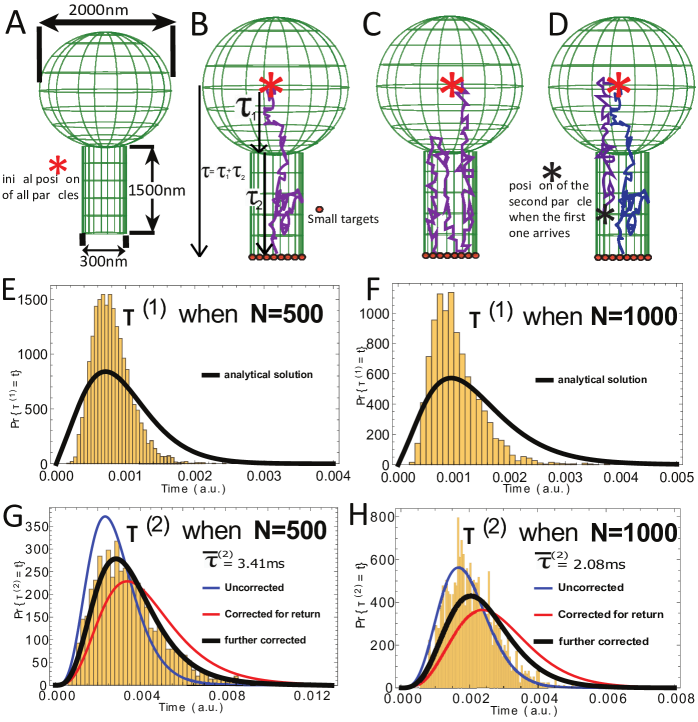
Figure 6: A-B-C-D: The geometry of the spine is a spherical head and cylindrical neck. Particles are released at the center of the head and must first reach the top of the neck and then diffuse through the neck to reach the base. Time taken for each process is represented with the notation $\tau_{1}$ and $\tau_{2}$, making the total time to be $\tau=\tau_{1}+\tau_{2}$. C shows a trajectory that can return to the head. Note that in D, when the first particle arrives, the second one, which could have return to the head, is now located inside the neck. E-F. Plot of $\Pr\{\tau^{(1)}=t\}$ for values $N=500,1000$. G-H. Plot of $\Pr\{\tau^{(2)}=t\}$ for values $N=500,1000$. The analytical solution is that of (158). Returns are accounted for with (165). The further corrected curve (black) is given by 166. The diffusion coefficient is $D=600\mu m^{2}/s$

Finally, the arrival time formula 165 can be further correct by adding the distribution of the particle inside the head. The correction is similar to the one we obtain in dimension one (formula 3.2 and 35). It can be written here using the survival probability 156 as

$$f^{(2)}_{further}(t)=\Pr\{\tau^{(2)}=t\}=N\int\limits_{0}^{t}f^{(1)}_{min}(t-s)f^{(1)}_{min}(s)J(t)^{N-1}ds.$$ (166)

8 Conclusion and applications of extreme statistics to fast time scale activation in cell biology

We derived here new asymptotics for the expected arrival time of fastest Brownian particles in several geometries: half a line, a segment, a bounded domain in dimension two and three that contains a small window, and spine-shaped geometry (a ball connected to thin cylinder). We found that the geometry is involved and explored by the fastest particle and the pdf is defined by the shortest ray (with reflections if the is an obstacle [20]) from the source to the target, in contrast with the narrow escape problem [17], where the main geometrical feature is the size of the window and the surface or volume of the domain. We derived here new laws for the first arrival time of Brownian particles to a target, which can be summarized as

$$\bar{\tau}^{d1} = \displaystyle\frac{\delta^{2}_{min}}{4D\ln(\frac{N}{\sqrt{\pi}})},\hbox{ in dim }1$$ (167)

$$\bar{\tau}^{d2} \approx \displaystyle\frac{\displaystyle s_{2}^{2}}{\displaystyle 4D\log\left(\frac{\pi\sqrt{2}N}{8\log\left(\frac{1}{\varepsilon}\right)}\right)},\hbox{ in dim }2$$ (168)

$$\bar{\tau}^{3d} \approx \frac{\delta^{2}_{m}}{2D\sqrt{\log\left(\displaystyle N\frac{4a^{2}}{\pi^{1/2}\delta^{2}}\right)}},\hbox{ in dim }3,$$ (169)

where $\delta_{min}$ is the shortest ray from the source to the window, $D$ is the diffusion coefficient and $N$ is the number of particles, $s_{2}=|\mbox{\boldmath$x$}-\mbox{\boldmath$A$}|$ and $x$ is the position of injection and the center of the window is $A$. Formula (167) is very different from the classical NET, which involves volume or surface area and mean curvature (in dimension 3). When the window is located at the end of a cusp, the asymptotics for the fastest particle are yet unresolved.

We further found that the rate of arrival cannot be approximated as Poissonian, because the fastest particle can arrive at a time scale that can fall into the short-time asymptotic. We further studied here the arrival of a second particle. The mean arrival time of the second can be influence by the distribution of all particles, especially on a segment, because the distribution of particles at the time the first particle’s arrival is not Dirac’s delta function (see section 3). However, the case of a spine geometry is interesting, because the first particle may have already arrived, but all other particles can still be in the head (due to the narrow opening at the neck-head connection). We further computed the pdf of the arrival time when particle can return to the head after sojourn in the neck (see section 7.2).

The present asymptotics have several important applications: activation of molecular processes are often triggered by the arrival of the first particles (ions or molecules) to target-binding sites. The simplest model of the motion of calcium ions in cell biology, such as neurons or a dendritic spine (neglecting electrostatic interactions) is that of independent Brownian particles in a bounded domain. The first two calcium ions that arrive at channels (such as TRP) can trigger the first step of biochemical amplification leading to the photoresponse in fly photoreceptor. Another example is the activation of a Ryanodine receptor (RyaR), mediated by the arrival of two calcium ions to the receptor binding sites, which form small targets. Ryanodin receptors are located at the base of the dendritic spine. Computing the distribution of arrival times of Brownian particles at the base, when they are released at the center of the spine head, is a model of calcium release during synaptic activation. Computing the distribution of arrival time reveals that the fastest ions can generate a fast calcium response following synaptic activity. Thus the fastest two calcium ions can cross a sub-cellular structure, thus setting the time scale of activation, which can be much shorter than the time defined by the classical forward rate, usually computed as the steady-state Brownian flux into the target, or by the narrow escape time [17].

References

• [1] C. Guerrier, E. Korkotian, D. Holcman, Calcium dynamics in neuronal microdomains: Modeling, stochastic simulations, and data analysis, Encyclopedia of Computational Neuroscience (2015) 486–516.
• [2] N. Volfovsky, H. Parnas, M. Segal, E. Korkotian, Geometry of dendritic spines affects calcium dynamics in hippocampal neurons: theory and experiments, Journal of neurophysiology 82 (1) (1999) 450–462.
• [3] D. Holcman, Z. Schuss, E. Korkotian, Calcium dynamics in dendritic spines and spine motility, Biophysical journal 87 (1) (2004) 81–91.
• [4] B. Katz, O. Voolstra, H. Tzadok, B. Yasin, E. Rhodes-Modrov, J.-P. Bartels, L. Strauch, A. Huber, B. Minke, The latency of the light response is modulated by the phosphorylation state of drosophila trp at a specific site, Channels 37 (2017) 1–8.
• [5] O. P. Gross, E. N. Pugh, M. E. Burns, Calcium feedback to cgmp synthesis strongly attenuates single-photon responses driven by long rhodopsin lifetimes, Neuron 76 (2) (2012) 370–382.
• [6] J. Reingruber, J. Pahlberg, M. L. Woodruff, A. P. Sampath, G. L. Fain, D. Holcman, Detection of single photons by toad and mouse rods, Proceedings of the National Academy of Sciences 110 (48) (2013) 19378–19383.
• [7] B. Hille, et al., Ion channels of excitable membranes, Vol. 507, Sinauer Sunderland, MA, 2001.
• [8] I. M. Sokolov, R. Metzler, K. Pant, M. C. Williams, First passage time of n excluded-volume particles on a line, Physical Review E 72 (4) (2005) 041102.
• [9] A. Zilman, G. Bel, Crowding effects in non-equilibrium transport through nano-channels, Journal of Physics: Condensed Matter 22 (45) (2010) 454130.
• [10] S. B. Yuste, K. Lindenberg, Order statistics for first passage times in one-dimensional diffusion processes, Journal of statistical physics 85 (3) (1996) 501–512.
• [11] S. B. Yuste, L. Acedo, K. Lindenberg, Order statistics for d-dimensional diffusion processes, Physical Review E 64 (5) (2001) 052102.
• [12] S. N. Majumdar, A. Pal, Extreme value statistics of correlated random variables, arXiv preprint arXiv:1406.6768.
• [13] T. Chou, M. D’orsogna, First passage problems in biology, First-Passage Phenomena and Their Applications 35 (2014) 306.
• [14] P. Krapivsky, S. N. Majumdar, A. Rosso, Maximum of n independent brownian walkers till the first exit from the half-space, Journal of Physics A: Mathematical and Theoretical 43 (31) (2010) 315001.
• [15] G. Schehr, Extremes of n vicious walkers for large n: application to the directed polymer and kpz interfaces, Journal of Statistical Physics 149 (3) (2012) 385–410.
• [16] S. Redner, B. Meerson, First invader dynamics in diffusion-controlled absorption, Journal of Statistical Mechanics: Theory and Experiment 2014 (6) (2014) P06019.
• [17] D. Holcman, Z. Schuss, Stochastic narrow escape in molecular and cellular biology, Analysis and Applications. Springer, New York.
• [18] D. Holcman, Z. Schuss, The narrow escape problem, SIAM Review 56 (2) (2014) 213–257.
• [19] Y. Colin de Verdière, Spectre du laplacien et longueurs des géodésiques périodiques i, Compos. Math 27 (1) (1973) 83–106.
• [20] Z. Schuss, A. Spivak, On recovering the shape of a domain from the trace of the heat kernel, SIAM Journal on Applied Mathematics 66 (1) (2005) 339–360.
• [21] Z. Schuss, Diffusion and stochastic processes: an analytical approach, Springer series on Applied mathematical sciences 170.
• [22] D. Holcman, Z. Schuss, Escape through a small opening: receptor trafficking in a synaptic membrane, Journal of Statistical Physics 117 (5) (2004) 975–1014.
• [23] M. Abramowitz, I. A. Stegun, Handbook of mathematical functions: with formulas, graphs, and mathematical tables, Vol. 55, Courier Corporation, 1964.
• [24] W. Chen, M. J. Ward, The stability and dynamics of localized spot patterns in the two-dimensional gray–scott model, SIAM Journal on Applied Dynamical Systems 10 (2) (2011) 582–666.
• [25] Z. Schuss, Brownian dynamics at boundaries and interfaces, Springer, 2015.