Intensity-Coupled-Polarization in Instruments with a Continuously Rotating Half-Wave Plate

Abstract

We discuss a systematic effect associated with measuring polarization with a continuously rotating half-wave plate. The effect was identified with the data from the E and B Experiment (EBEX), which was a balloon-borne instrument designed to measure the polarization of the CMB as well as that from Galactic dust. The data show polarization fraction larger than 10% while less than 3% were expected from instrumental polarization. We give evidence that the excess polarization is due to detector non-linearity in the presence of a continuously rotating HWP. The non-linearity couples intensity signals into polarization. We develop a map-based method to remove the excess polarization. Applying this method for the 150 (250) GHz bands data we find that 81% (92%) of the excess polarization was removed. Characterization and mitigation of this effect is important for future experiments aiming to measure the CMB B-modes with a continuously rotating HWP.

1 Introduction

Measurements of the cosmic microwave background (CMB) temperature and polarization provide a window on the physical mechanisms that govern the evolution of the Universe. The EBEX was a balloon-borne telescope designed to measure the polarization of the CMB while simultaneously measuring Galactic foreground emission. EBEX achieved polarimetry via a stationary wire-grid polarizer and a continuously rotating achromatic half-wave plate (HWP). The use of a continuously rotating HWP to modulate incident polarized radiation is a well-known polarimetric technique (see, e.g., Johnson et al. (2007); Kusaka et al. (2014)). Continuous modulation of polarized signals is useful for mitigating systematic errors in two ways. It reduces the impact of low frequency noise in the detectors by moving the polarization signal of interest to a higher frequency band, where the detector noise is primarily white. In addition, it enables measurement of both the $Q$ and $U$ Stokes polarization parameters without differencing polarization sensitive detectors. Differencing of signals among detector pairs requires the responsivity and noise to be stable and well characterized, while mismatching of the detector beams is a source of systematic error such as intensity to polarization signal coupling (Shimon et al., 2008; BICEP2 Collaboration et al., 2015).

A common concern for experiments measuring B-modes, which is a curl pattern in the polarization of the CMB, is intensity coupling to the polarization signal, that we refer to as intensity-coupled-polarization (ICP). Intensity signals from the CMB and from foreground sources (including the atmosphere for ground based experiments) can be orders of magnitude larger than CMB polarization signals. Even low levels of ICP add systematic bias to the polarization signal and can induce low frequency noise if the intensity is time variable. A common source of ICP is instrumental polarization (IP). Here IP is used in the traditional sense referring to the conversion of intensity to polarization through differential transmission or reflection in optical elements. Another common source of ICP is beam and responsivity mismatch between detector pairs. Using a continuously rotating HWP can mitigate these sources of ICP: the IP is reduced because only optical elements sky-side of the HWP contribute to it, and the pair differencing effects are avoided because polarization is measured without differencing detector pairs (Kusaka et al., 2014; Essinger-Hileman et al., 2016; Takakura et al., 2017).

The subject of this paper is the analysis of a new mechanism for creating ICP in EBEX, generated by detector non-linearity in the presence of a rotation synchronous signal generated by a HWP. A similar effect has been reported in Takakura et al. (2017). Understanding and mitigating this effect will be important for future CMB missions using a continuously rotating HWP. This paper describes the excess intensity coupled polarization (ICP) observed in EBEX maps, outlines two possible sources for the excess polarization (IP and detector non-linearity), uses data to distinguish between those two origins, and details the method we developed to characterize and remove the excess polarization. Because the magnitude of this ICP is correlated with a rotation synchronous signal generated by the HWP, we also discuss sources of this rotation synchronous signal.

The paper is organized as follows. In Section 2 we outline the data model of an experiment with a continuously rotating HWP. EBEX maps showing excess polarization are shown in Section 3. In Section 4 we provide two models for the physical origins of the ICP. In Section 5 we describe in detail the physical origins of the HWP synchronous signal. In Section 6 we characterize the ICP for each EBEX detector and show with this measurement that we can distinguish between various ICP mechanisms. In Section 7 we present the method we developed to remove the ICP and evaluate its performance on real and simulated data.

2 Data model

The instrument is modelled by an achromatic HWP and a wire grid analyzer. The HWP is rotating at a constant speed (in EBEX the rotational frequency was 1.235 $\mathrm{Hz}$) and we call $\gamma_{t}$ the angle between the HWP extraordinary axis and the polarizing grid, where the subscript $t$ is used to indicate time-dependence. For a given Stokes vector $\vec{S}^{in}_{t}$ incident on the receiver, the output Stokes vector $\vec{S}^{out}_{t}$ at the detectors (integrated over the detector bandwidth) is

$$\vec{S}^{out}_{t} =M_{instr}\,\vec{S}^{in}_{t}$$ (1)

$$=M_{lp}\,M_{HWP}(\gamma_{t})\left(\begin{array}[]{c}I^{in}_{t}\\ Q^{in}_{t}\\ U^{in}_{t}\\ 0\\ \end{array}\right)$$ (6)

$$M_{instr}=M_{lp}\,M_{HWP}(\gamma_{t}) =\frac{1}{2}\,\left(\begin{array}[]{cccc}1&\epsilon\cos(4\gamma_{t}\!-\!\Phi_{t})&\epsilon\sin(4\gamma_{t}\!-\!\Phi_{t})&0\\ 1&\epsilon\cos(4\gamma_{t}\!-\!\Phi_{t})&\epsilon\sin(4\gamma_{t}\!-\!\Phi_{t})&0\\ 0&0&0&0\\ 0&0&0&0\\ \end{array}\right)$$

where $M_{lp}$ and $M_{HWP}(\gamma_{t})$ are the Mueller matrices of a linear polarizer and a HWP, respectively, $\epsilon$ is the HWP polarization modulation efficiency, and $\Phi_{t}$ is an angle encoding the offset between the sky-fixed $Q$ & $U$ reference frame and the polarizing grid, as well as the frequency dependent phase delay introduced by the achromatic HWP (Johnson et al., 2007; Matsumura, 2006). Details on the coordinates and the instrument and sky frames used throughout the paper are available in Appendix A. The detectors are only sensitive to power $I^{out}_{t}$ computed from Equation 1, and their time-stream $D_{t}$ is:

$$D_{t} =I^{out}_{t}$$ (8)

$$=\frac{1}{2}\,\Big{(}I^{in}_{t}+\epsilon Q^{in}_{t}\cos(4\gamma_{t}-\Phi_{t})+\epsilon U^{in}_{t}\sin(4\gamma_{t}-\Phi_{t})\Big{)}$$

We separate the incoming Stokes vector $\vec{S}^{in}_{t}$ into the desired sky signal $\vec{S}^{sky}_{t}$ and $\vec{S}^{instr}_{t}$ which corresponds to spurious unpolarized and polarized signals from the instrument, giving:

$$D_{t}= \,\frac{1}{2}\,\Big{(}I^{sky}_{t}+\epsilon Q^{sky}_{t}\cos(4\gamma_{t}-\Phi_{t})+\epsilon U^{sky}_{t}\sin(4\gamma_{t}-\Phi_{t})\Big{)}$$

$$+A(\gamma_{t})+n_{t}$$ (9)

where $n_{t}$ is the detector noise and $A(\gamma_{t})$ groups spurious instrument signals $\vec{S}^{instr}$ modulated by the HWP. The spurious modulation signal, called from hereafter the HWP Synchronous Signal, or HWPSS, is modeled by:

$$A(\gamma_{t})=\sum\limits_{j=0}^{\infty}\quad\underbrace{A_{j}\cos(j\gamma_{t}-2\alpha_{j})}_{\text{stationary}}\quad+\quad\underbrace{A^{\prime}_{j}I^{sky}_{t}\cos(j\gamma_{t}-2\alpha^{\prime}_{j})}_{\text{scan modulated}}$$ (10)

where we have distinguished between stationary HWPSS emitted by the instrument and scan modulated HWPSS coupled to $I_{t}^{sky}$. All spurious effects are lumped into the $A_{j}$, $A^{\prime}_{j}$, $\alpha_{j}$ and $\alpha^{\prime}_{j}$ parameters and are phenomenologically allowed to be present at all harmonics $j$. To account for time-dependant temperature fluctuations in the instrument, the parameters are allowed to vary linearly with time.

The 4th harmonic amplitude terms ($A_{4}$ and $A^{\prime}_{4}$) represent instrumentally induced polarized power. This category includes:

• the stationary signals represented by $A_{4}$ such as instrument polarized emissions and instrument unpolarized emissions polarized through IP. Instrument polarized and unpolarized emission are stationary in that they vary only with thermal variations in the instrument. As such the $A_{4}$ term, though it represents the largest polarization signal measured by the detectors (see Section 5), is separable from the sky polarization because it is constant over timescales on which the instrument is thermally stable.

• scan modulated signals represented by $A^{\prime}_{4}I^{sky}$ which we call in this paper ICP. ICP includes two effects: IP acting on $I^{sky}$ that we label ICP^IP, but also ICP arising from non-linear detector response which is the subject of this paper and that we label ICP^NL.

In the next section we show the ICP observed in EBEX maps. In Section 4 we describe in more details the physical mechanisms generating ICP^IP and ICP^NL.

3 Intensity-Coupled-Polarization (ICP) Observed in EBEX Maps

3.1 The EBEX Instrument

A detailed description of the instrument is available in The EBEX Collaboration (2017a, b, c). We provide here a summary relevant to the understanding of the origin of the ICP. The EBEX instrument was a balloon-borne telescope designed to measure the E- and B-mode polarization of the CMB while simultaneously measuring Galactic dust emission over the range 30 $<$ $\ell$ $<$ 1500 of the angular power spectrum. To achieve sensitivity to both the CMB polarization signal and galactic foregrounds, EBEX had three bands centered on 150, 250, and 410 GHz.

The telescope optics comprised warm primary and secondary mirrors and a series of cold lenses and filters located inside a cryogenically cooled receiver (see Figure 1). EBEX achieved polarimetry via a stationary wire-grid polarizer and a 24 cm diameter continuously rotating achromatic HWP composed of a stack of five birefringent sapphire disks following a Pancharatnam design (Pancharatnam, 1955). Incoming optical rays were focused onto each focal plane by a field lens and a series of pupil and camera lenses. The HWP was kept at 4 $\mathrm{K}$ and located at an aperture stop such that each detector beam covered the HWP. The field lens was located at an image of the focal plane. Each focal plane contained an array of transition-edge sensor (TES) bolometric detectors arranged into seven hexagonal wafers, with four 150 GHz wafers, two 250 GHz wafers, and one 410 GHz wafer per focal plane. EBEX operated 955 detectors during its science flight.

EBEX launched from McMurdo station, Antarctica on December 29, 2012, circumnavigating the continent at an altitude of $\sim$ 35 km and landing 25 days later on January 23, 2013. We refer to data from this flight as EBEX2013. The cryogenic system that cooled the receiver was active for 11 days before cryogens depleted. Due to an error in thermal modelling (The EBEX Collaboration, 2017b), EBEX was unable to point in azimuth and as a result EBEX scanned a 5,700 deg² strip of sky delimited by declination $-67.9^{\circ}$ and $-38.9^{\circ}$, corresponding to free rotations in azimuth at a constant elevation of 54$\mathrm{\SIUnitSymbolDegree}$.

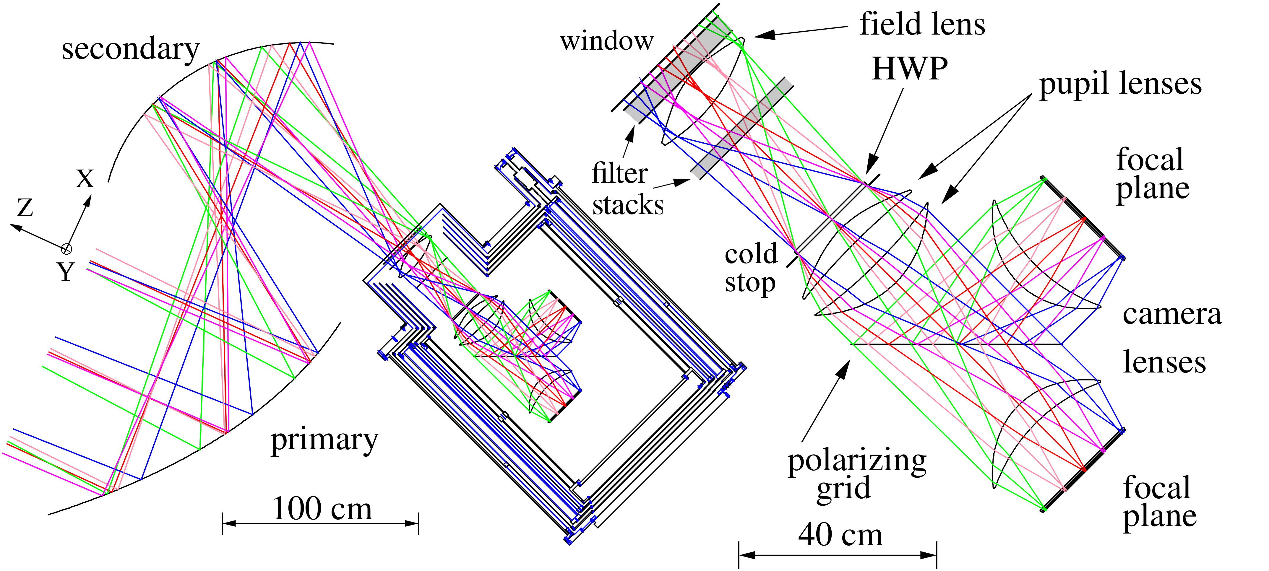
Figure 1: Ray tracing of the EBEX optical design consisting of two ambient temperature reflectors in a Gregorian configuration and a cryogenic receiver (left). Inside the receiver (right), cryogenically cooled polyethylene lenses formed a cold stop and provided diffraction limited performance over a flat, telecentric, $6.6\text{\,}\mathrm{\SIUnitSymbolDegree}$ field of view.

3.2 EBEX Maps

We present here maps from EBEX2013 data and show that we observe ICP. To make maps we remove the stationary part of the HWPSS, calibrate, deconvolve the detector time-constant, demodulate and filter the time-streams to extract $I$, $Q$ and $U$ and bin them into pixels. A detailed review of the time-stream processing is available in Didier (2016) and Araujo (2017), and the calibration is described in Aubin et al. (2016). Figure 2 shows Planck and EBEX maps of the bright embedded cluster RCW38 for Stokes $I$ and the polarization power $P$, defined as $P=\sqrt{Q^{2}+U^{2}}$. Polarization orientation is reconstructed in the instrument frame (see definition in Appendix A). Planck maps closest in frequency to the EBEX bands are first smoothed to the EBEX beam size. Planck time-streams are then generated using the EBEX pointing and HWP angles, and those time-streams are processed and binned into maps using the same pipeline as EBEX2013 time-streams. Excess polarization in the EBEX data is apparent for both 150 and 250 GHz maps. The $I$ to $P$ Pearson correlation coefficient and linear slope are given in Table 1. The high correlation coefficient between $I$ and $P$ points to the excess polarization in EBEX2013 coming from ICP. The measured linear slopes of 11% (12%) for 150 (250) GHz correspond to a measurement of $A^{\prime}_{4}$ (from Equation 10) averaged over detectors. These numbers are larger than the maximum anticipated IP of 2.7% as will be explained in Section 4.1.

RCW 38 CMB Stacked Spots Correlation Linear Correlation Linear Coefficient Slope (%) Coefficient Slope (%) Planck 143 GHz 0.1 0.2 0.3 0.0 EBEX 150 GHz 0.8 11 0.8 8 Planck 217 GHz 0.3 0.7 0.2 0.1 EBEX 250 GHz 0.8 12 0.6 16

Table 1: Pearson correlation and linear slope (corresponding to an average of $A^{\prime}_{4}$ across detectors) between $I$ and $P$ using RCW38 and stacked CMB maps. For RCW38, only pixels with $I$ greater than 2 (9) $\mathrm{mK}$ are used for 150 (250) GHz calculations. For CMB, only pixels with $I$ greater than 10 $\mathrm{\SIUnitSymbolMicro K}$ are used for calculations. We estimate the one sigma error on the slope to be 1% for EBEX data and 0.1% for Planck data.

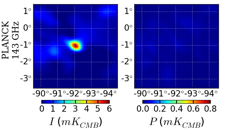
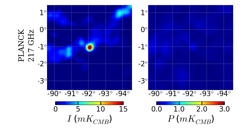
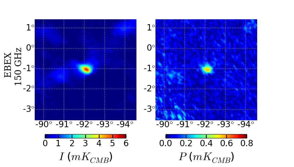
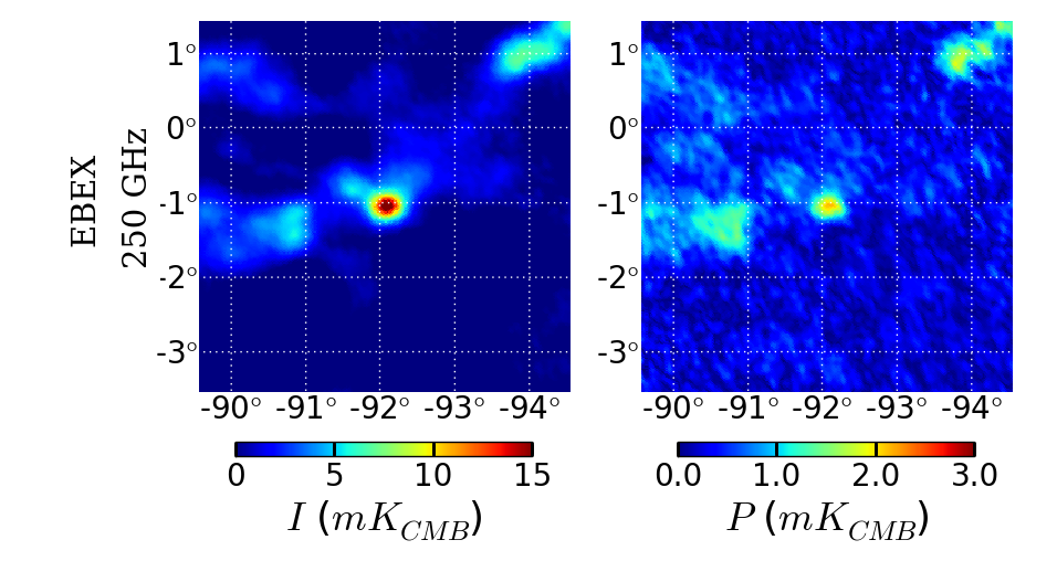
Figure 2: Comparison of RCW38 maps in $I$ and $P$ between Planck at 143 GHz (top left), EBEX at 150 GHz (bottom left), Planck at 217 GHz (top right) and EBEX at 250 GHz (bottom right). The maps shown in Galactic coordinates co-add 332 (216) detectors at 150 (250) GHz. The polarization orientation is reconstructed in the instrument frame.

We ascertain the existence of ICP by co-adding maps around CMB cold and hot spots (Komatsu et al., 2011). We identify spot locations by examining the Planck CMB maps (see Didier (2016)). We smooth the EBEX $I$, $Q$, $U$ maps to 0.5$\mathrm{\SIUnitSymbolDegree}$ ($Q$, $U$ are oriented in the instrument frame) and extract a square region of 5$\mathrm{\SIUnitSymbolDegree}$ $\times$ 5$\mathrm{\SIUnitSymbolDegree}$ around the spot extremum. The hot and cold spots are stacked. Figures 4 and 4 show the resulting stacked spots from co-adding $\sim$2000 spots using 150 and 250 GHz detectors, respectively. We show the stacked spots in $I$ and also in polarization power $P$ made from the $Q$ and $U$ stacked spots. In both EBEX and Planck, the CMB is visible in the co-added $I$ maps. For polarization co-added in the instrument frame coupled to the EBEX scan strategy, we expect no CMB polarization power in the stacked spots, and none is observed in the Planck $P$ data. In EBEX, polarization power is visible in the center of the stacked $P$ map, this is the result of ICP. The correlation coefficient and linear slope between $I$ and $P$ are shown in Table 1 and the EBEX numbers are consistent between the RCW38 and CMB stacked map measurements. In the next section, we describe in more details the two mechanisms (IP and detector non-linearity) responsible for ICP.

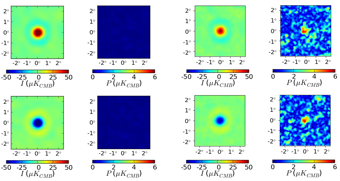
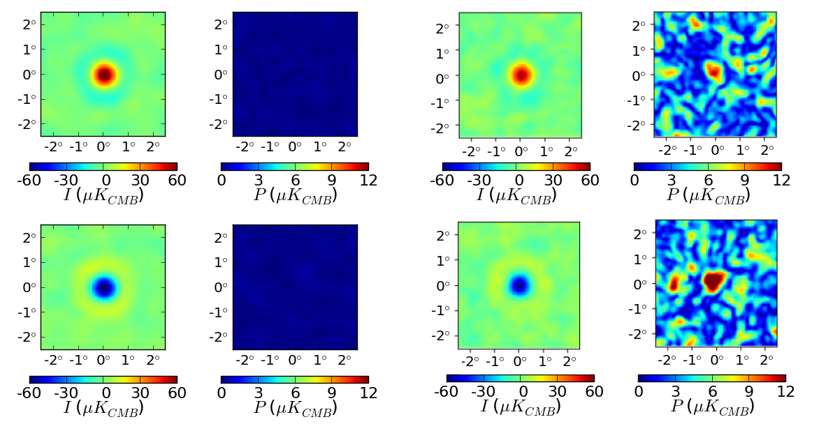
Figure 3: Co-added CMB hot and cold spots for Planck 143 GHz (left four) and EBEX 150 GHz (right four) in $I$ and $P$. For each experiment, hot (cold) spots are shown on top (bottom) and co-add 2122 (2255) spots.

Figure 4: Co-added CMB hot and cold spots for Planck 217 GHz (left four) and EBEX 250 GHz (right four) in $I$ and $P$. For each experiment, hot (cold) spots are shown on top (bottom) and co-add 1918 (2092) spots.

4 Mechanisms for Intensity-Coupled-Polarization (ICP)

We examine here two physical mechanisms responsible for ICP and trace the amplitude and polarization angle of each as a function of focal plane position. This provides a way to distinguish between them.

4.1 Instrumental Polarization (IP)

Mirror and lenses sky-side of the HWP are typical sources of IP in CMB instruments. Unpolarized radiation $I^{sky}$ incident on the instrument will produce an ICP^IP signal $I^{sky}\,\varepsilon^{IP}\,\cos(4\gamma_{t}-2\alpha^{IP})$ that has polarization fraction $\varepsilon^{IP}$ and polarization angle $\alpha^{IP}$, where $\varepsilon^{IP}$ and $\alpha^{IP}$ are determined by the instrument configuration.

In EBEX, the optical design software Code V shows that the main source of IP is the field lens, dominating the mirror IP by an order of magnitude at 150 and 250 GHz. Figure 1 shows the location of and incident rays on the field lens. The amount of IP from the field lens increases with distance $d$ away from the lens center because of the increasing incident angles from the lens curvature. Unpolarized radiation $I^{sky}$ incident on the lens will be polarized in the plane of incident light (see Appendix B for a general derivation). Over all rays hitting the field lens at a given location forming an angle $\beta$ with the x-axis, the outgoing polarization will have a polarization angle $\alpha^{IP}=\beta$.

The EBEX field lens is located at an image of the focal plane such that the IP properties directly translate to the focal plane. Let the polar coordinates of a detector on the focal plane be its radial distance from the center $r_{det}$ and its polar angle $\rho_{det}$. The detector illuminated by a ray hitting the field lens at radius $d$ and angle $\beta$ is the detector with coordinates $r_{det}=d$ and $\rho_{det}=\beta$. Therefore the ICP^IP of each detector has polarization angle $\alpha^{IP}$ equal to the polar angle $\rho_{det}$ of the detector position on the focal plane, and polarization fraction $\varepsilon^{IP}$ which increases for a detector at the edge of the focal plane. Code V modelling for EBEX shows a maximum polarization fraction $\varepsilon^{IP}$ of $2.7$ % at the edge of the focal plane for the 150 and 250 GHz frequency bands (The EBEX Collaboration, 2017c).

If IP is the dominant source of ICP in EBEX, we expect $A^{\prime}_{4}$ (from Equation 10) to be of order $\varepsilon^{IP}\sim 2.7\%$ given Code V predictions , and the ICP polarization angle $\alpha^{\prime}_{4}$ to be equal to the IP polarization angle $\alpha^{IP}$ which in EBEX is equal to the detector polar angle $\rho_{det}$. Future experiments wishing to mitigate ICP^IP can diminish the magnitude of $\varepsilon^{IP}$ by placing the HWP at the beginning of the optical chain: only optical elements sky-side of the HWP contribute to the total IP.

4.2 Detector Non-Linearity

Another possible source of ICP is detector non-linearity in the presence of a HWPSS with a 4th harmonic.

We derive the properties of the ICP^NL using a simplified version of the data model in Equation 9 in which the incoming power on the detectors is composed solely of an unpolarized sky signal and a stationary 4th harmonic HWPSS parametrized by $A_{4}$:

$$D_{t}=I^{sky}_{t}+A_{4}\cos(4\gamma_{t}-2\alpha_{4}).$$ (11)

Let $D_{t}$ vary over a range larger than the linear range of the detector response. For this derivation, we limit our non-linearity model to second order terms and ignore time-constant effects. We write the non-linear detector response as

$$D^{NL}_{t}=f^{NL}(D_{t})=D_{t}-KD_{t}^{2}$$ (12)

where $K$ has unit of inverse power and characterizes the non-linearity of the detector. For TES detectors tuned in the high-resistance regime of their superconducting transition, we can assume $K>0$, as we show in Appendix C. We now re-write the detector time-stream as:

$$D^{NL}_{t}= \,f^{NL}\big{(}I^{sky}_{t}+A_{4}\cos(4\gamma_{t}-2\alpha_{4})\big{)}$$

$$= \,(1-KI^{sky}_{t})I^{sky}_{t}$$

$$+2A_{4}K\,I^{sky}_{t}\,\cos(4\gamma-2(\alpha_{4}+\frac{\pi}{2}))$$

$$+A_{4}\cos(4\gamma-2\alpha_{4})$$

$$-\frac{1}{2}KA_{4}^{2}\cos(8\gamma-4\alpha_{4})-\frac{1}{2}KA_{4}^{2}.$$ (13)

The non-linear response has multiple effects:

• it decreases $I^{sky}_{t}$ by $(1-KI^{sky}_{t})$;

• it creates an ICP^NL signal $2A_{4}KI^{sky}_{t}\cos(4\gamma-2(\alpha_{4}+\frac{\pi}{2}))$, with polarization fraction $\varepsilon^{NL}=2A_{4}K$ and polarization angle $\alpha^{NL}=\alpha_{4}+\frac{\pi}{2}$;

• it creates higher harmonics in the HWPSS (in this second order example, only an 8th harmonic), as well as modify the DC level.

Our model does not include intrinsic sky polarization $P^{sky}_{t}$, but one can show similarly that non-linearity decreases $P^{sky}_{t}$ by $(1-2KI^{sky}_{t})$.

If non-linearity is the dominant source of ICP in EBEX, we expect $A^{\prime}_{4}$ to be of order $\varepsilon^{NL}=2A_{4}K$, and the ICP polarization angle $\alpha^{\prime}_{4}$ to be equal to the non-linear model polarization angle $\alpha^{NL}$ which is offset from the stationary HWPSS 4th harmonic polarization angle $\alpha_{4}$ by $\frac{\pi}{2}$. Note that because the polarization fraction of ICP^NL is determined by the product of $A_{4}$ and the detector non-linearity $K$, future experiments wishing to minimize ICP^NL can act on both the non-linearity of the detectors ($K$) and the magnitude of the stationary HWPSS 4th harmonic ($A_{4}$), the latter by minimizing the polarized and unpolarized thermal emissions sky side of the HWP.

To determine the origin of the ICP observed in EBEX, we can measure the ICP polarization angle $\alpha^{\prime}_{4}$ and compare it to both $\rho_{det}$ and to the stationary HWPSS polarization angle $\alpha_{4}$. In Section 6 we use the data to show that the ICP polarization angle $\alpha^{\prime}_{4}$ is consistent with a non-linear origin of the signal, and is not consistent with IP as its origin. We first determine the properties of the stationary HWPSS.

5 Stationary HWP Synchronous Signal

In Figure 5 we plot a detector time-stream and power spectral density (PSD) from EBEX, showing that a HWPSS dominates the detector time-streams. The HWPSS has power at all harmonics of the HWP rotation up to the Nyquist frequency, with the 4th harmonic being the dominant harmonic by an order of magnitude. The stationary part of the HWPSS (coefficients $A_{j}$, $\alpha_{j}$ in Equation 10) is fitted using a maximum likelihood estimator. We refer the reader to Didier (2016) and Araujo (2017) for a detailed review on the stationary HWPSS fitting and removal. The power in $A_{4}$ comes from two sources sky side of the HWP: unpolarized power (thermal instrument emission, CMB monopole and atmosphere) getting polarized through IP, as well as polarized thermal emission from the instrument.

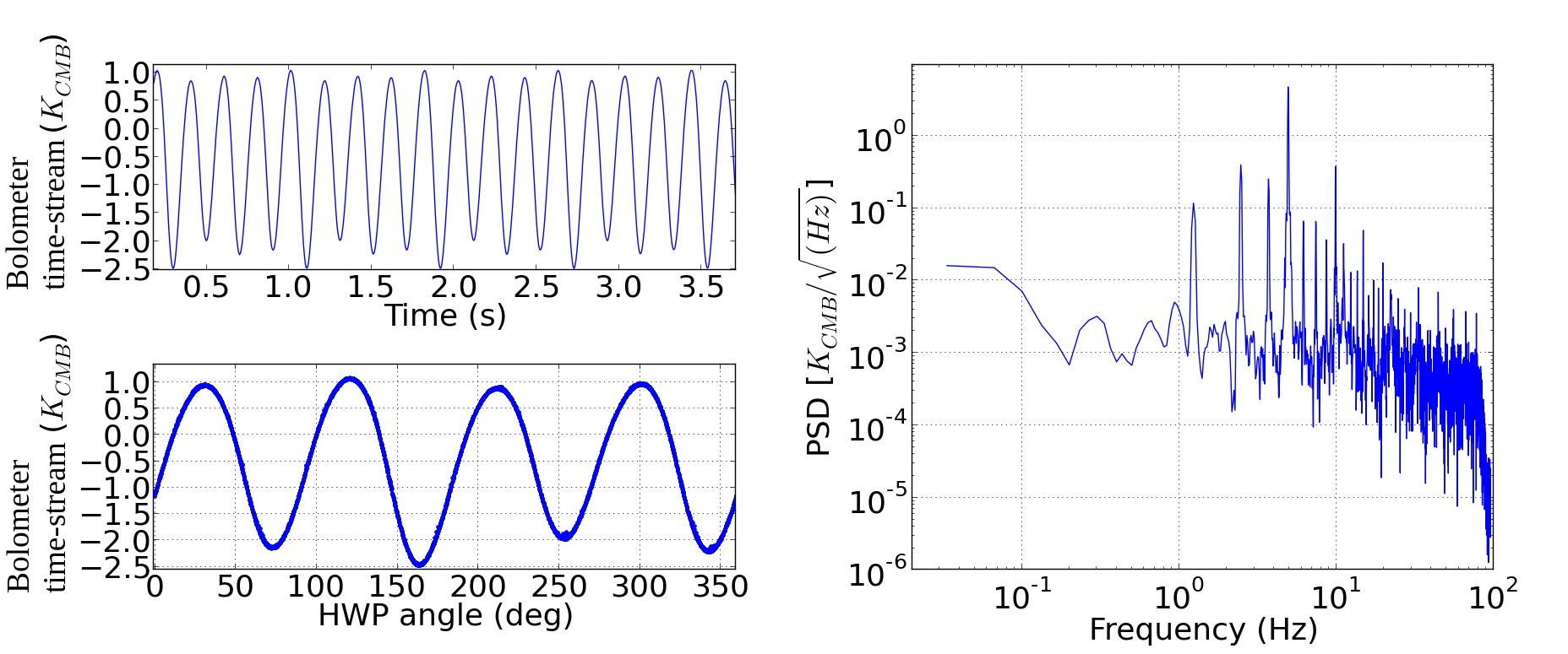
Figure 5: Left, top: Plot of a calibrated detector time-stream over 3.5 $\mathrm{s}$ of data prior to stationary HWPSS removal. The HWPSS has amplitude of 3.5 $\mathrm{K}$ and dominates the signal. Left, bottom: Plot of the same detector time-stream versus HWP angle, showing the HWPSS is synchronous with the HWP rotation. The 4th harmonic dominates the HWPSS. Right: PSD of the same detector time-stream.

5.1 Unpolarized Thermal Emission Polarized Through IP

In Section 4.1 we showed how IP acts on $I^{sky}$ to produce ICP^IP. Similarly, IP will act on $I^{instr}$ to produce a stationary polarized signal. As discussed earlier, in EBEX because the dominant source of IP is the field lens located at an image of the focal plane, polarization signals generated by IP will exhibit a distinctive pattern as a function of focal plane position: the polarization angle will be equal to the polar angle of the detector, and the polarized power will increase with radial distance away from the focal plane center ($A_{4}$ from IP is equal to $I^{instr}\varepsilon^{IP}$) . This is what we observe in the stationary HWPSS 4th harmonic, as shown in Figure 6 (top and bottom panel). This data indicates field lens IP is a dominant source of the stationary HWPSS 4th harmonic. Its magnitude is estimated in Table 2 by combining the thermal load on the detectors measured from flight with the IP predicted from Code V. We note that the load measured in flight was larger than what was predicted pre-flight. We hypothesize that the excess load comes from spillover onto warm, highly emissive surfaces around the mirrors, caused by diffraction around the aperture stop. The predicted and measured loads and a discussion of this effect are available in The EBEX Collaboration (2017a). The excess load increased the amount of unpolarized light passing through the field lens and therefore the HWPSS.

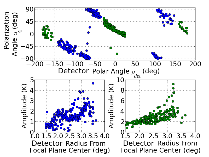
Figure 6: Top: Polarization angle $\alpha_{4}$ of the stationary HWPSS 4th harmonic for 150 (blue) and 250 (green) GHz detectors, plotted against the detector polar angle $\rho_{det}$ on the focal plane, showing strong 1:1 linear correlation between $\alpha_{4}$ and $\rho_{det}$ (the negative slope comes from using different conventions for $\alpha$ and $\rho_{det}$). Bottom: Amplitude $A_{4}$ of the stationary HWP 4th harmonic for 150 (left) and 250 (right) GHz detectors, plotted against the detector distance $r_{det}$ from the focal plane center. Within each frequency band, the amplitude of the HWPSS increases with detector radius.

5.2 Polarized Thermal Emission

Polarized thermal emission from the instrument also contributed to $A_{4}$. The dominant contribution of polarized thermal emission comes from the mirrors. The polarized fraction of mirror thermal emission $p^{emission}$ as a function of the angle of emission $\theta$ with respect to normal incidence is (Strozzi & McDonald, 2000):

$$p^{emission} =\frac{\sin^{2}(\theta)}{1+\cos^{2}(\theta)}$$ (14)

The range of angles of emission that couple to our detectors is identical to the range of incidence angles for our optics. For the primary mirror, this range is from $10^{\circ}$ to $45^{\circ}$, giving non-negligible polarization fractions. We average the polarization fraction across the beam for each of the mirrors, finding values for $p^{emission}$ of 16% and 6.4% at the center of the focal plane for the primary and secondary mirrors, respectively. The polarization angle $\alpha^{emis}$ of the polarized emission should be approximatively uniform across the focal plane, with $\alpha^{emis}\approx 0^{\circ}$. We observe $\alpha^{emis}$ to be non-zero in the top panel of Figure 6, indicating that polarized thermal emission is a sub-dominant contribution to the stationary HWPSS 4th harmonic.

5.3 Comparing Measurements to Model Predictions

Our estimate for the two contributions to the HWPSS (IP and polarized emission) is given in Table 2 along with the observed size of the HWPSS, all given in units of power incident on the telescope. We note that the HWPSS varies across detectors and we only provide here average measurements and predictions. In particular, the two contributions will add differently for different locations across the focal plane given the varying polarization angles.

	Estimated HWPSS	Predicted HWPSS
Frequency Band	size from field	size from polarized	Observed HWPSS
(GHz)	lens IP using	emission (fW)	size (fW)
	flight load (fW)
150	370	85	570
250	720	190	670
410	350	400	560

Table 2: HWPSS 4th harmonic amplitudes predictions and observations, expressed as power incident on the telescope. The conversion from power to CMB temperature is 3.24, 4.54 and 16.1 $mK_{CMB}/fW$ at 150, 250 and 410 GHz. The two sources of HWPSS don’t necessarily have the same polarization angle.

6 Single Detector Characterization of ICP

In this section we present a general method to characterize ICP coupling coefficients $A^{\prime}_{4}$ and $\alpha^{\prime}_{4}$ for each detector, independently of the ICP origin. The measurement of the coupling coefficients can inform the physical origin of the ICP and be used to remove the excess polarization.

In Equation 9 we showed that the power incident on a detector is the sum of the sky signal and the HWPSS, itself composed of a stationary term and a term modulated by the sky intensity $I_{t}^{sky}$. Having removed the stationary HWPSS term and now focusing on the dominant 4th harmonic, the detector time-stream becomes:

$$D^{TOTAL}_{t} \sim\frac{1}{2}\,\Big{(}I^{sky}_{t}+P^{sky}_{t}\cos(4\gamma_{t}-2\psi_{t}-2\alpha^{sky}_{t})\Big{)}+A^{\prime}_{4}I^{sky}_{t}\cos(4\gamma_{t}-2\alpha^{\prime}_{4})+n_{t}$$ (15)

$$=D^{sky}_{t}+D^{ICP}_{t}+n_{t}$$ (16)

where $D^{ICP}_{t}=A^{\prime}_{4}I^{sky}_{t}\cos(4\gamma_{t}-2\alpha^{\prime}_{4})$ stands for the ICP term, $\psi_{t}$ is the Galactic roll angle (see Appendix A for the transition from using $\Phi_{t}$ to $\psi_{t}$) and $n_{t}$ is the noise. We note that the polarization of $D^{ICP}_{t}$ originates in the instrument frame in contrast to the polarization of $D^{sky}_{t}$ which originates in the sky frame (hence its dependence on the Galactic roll angle $\psi_{t}$).

To isolate and measure $D^{ICP}$, we make single detector $I$, $Q$ and $U$ maps of $D^{TOTAL}$ in the instrument frame. The value of each pixel $p$ is:

$$I_{p} =\frac{\sum\limits_{t}w_{t}I^{sky}_{t}}{\sum\limits_{t}w_{t}}+n^{I}_{p}=I^{sky}_{p}+n^{I}_{p}$$ (17)

$$Q_{p} =Q^{sky}_{p}\frac{\sum\limits_{t}w_{t}\cos(2\psi_{t})}{\sum\limits_{t}w_{t}}+I^{sky}_{p}A^{\prime}_{4}\cos(2\alpha^{\prime}_{4})+n^{Q}_{p}$$ (18)

$$U_{p} =U^{sky}_{p}\frac{\sum\limits_{t}w_{t}\sin(2\psi_{t})}{\sum\limits_{t}w_{t}}+I^{sky}_{p}A^{\prime}_{4}\sin(2\alpha^{\prime}_{4})+n^{U}_{p}$$ (19)

where the summation is over all time samples $t$ pertaining to a given pixel $p$, $w_{t}$ are the map-making weights and $n^{[I,Q,U]}_{p}$ is the pixel noise. Here we used the usual transformation $Q^{sky}=P^{sky}\cos(2\alpha^{sky})$ and $U^{sky}=P^{sky}\sin(2\alpha^{sky})$. To measure the coupling parameters, an unpolarized source can be used ($Q^{sky}_{p}=U^{sky}_{p}=0$) or a polarized source can be sampled with varied Galactic roll such that $\sum w_{t}\cos(2\psi_{t})$ and $\sum w_{t}\sin(2\psi_{t})$ tend to zero. The coupling parameters for each detector are estimated from the maps using ensemble averages of $I_{p}$, $Q_{p}$ and $U_{p}$:

$$\tilde{A}^{\prime}_{4}=\frac{\sqrt{\langle Q_{p}\rangle^{2}+\langle U_{p}\rangle^{2}}}{\langle I_{p}\rangle}$$ (20)

$$\tilde{\alpha}^{\prime}_{4}=\frac{1}{2}\arctan(\frac{\langle U_{p}\rangle}{\langle Q_{p}\rangle})$$

where the tilde denotes the measured quantity. For EBEX, the three possible sources are the CMB, RCW38 and the Galactic plane. EBEX doesn’t have enough sensitivity to measure the CMB with single detectors. RCW38 is sampled with enough signal to noise but poor coverage. This leaves the Galaxy which has intrinsic polarization. For an extended source like the Galaxy, summing all the pixels within the source will increase the signal to noise and the sampling of $\psi_{t}$. Using simulations, we estimate the error on the coupling parameters coming from partial Galactic roll coverage to be 1.7% for $\tilde{A}^{\prime}_{4}$ and 3$\mathrm{\SIUnitSymbolDegree}$ for $\tilde{\alpha}^{\prime}_{4}$ for the EBEX scan strategy.

For each detector, we produce $I$, $Q$ and $U$ maps of the Galactic plane in the instrument orientation, with Healpix NSIDE 256 (Górski et al., 2005). We define as valid the pixels located within $\pm$3$\mathrm{\SIUnitSymbolDegree}$ of the Galaxy, and with Stokes $I$ value greater than or equal to 3 (15) $\mathrm{mK}$ for 150 (250) $\mathrm{GHz}$ detectors. We calculate for each detector the ensemble average $\langle I\rangle$, $\langle Q\rangle$ and $\langle U\rangle$ value by averaging all the valid pixels. Using those values and Equation 20 we estimate for each detector $\tilde{A}^{\prime}_{4}$ and $\tilde{\alpha}^{\prime}_{4}$, and plot the results in Figure 7. We observe that the coupling angle $\tilde{\alpha}^{\prime}_{4}$ varies linearly with the detector polar angle $\rho_{det}$, and that the coupling fractions $\tilde{A}^{\prime}_{4}$ are spread over a wide range with a mode of 7% and a median absolute deviation of 5.7%. These $\tilde{A}^{\prime}_{4}$ values are consistent with the RCW38 and CMB linear slopes reported in Table 1 corresponding to an average of $A^{\prime}_{4}$ over all detectors.

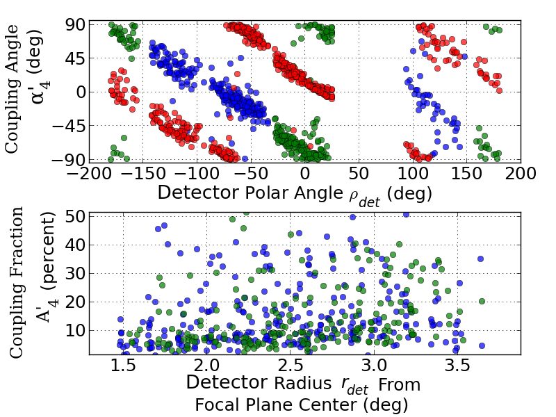
Figure 7: Top: Measurement of the coupling angle $\tilde{\alpha}^{\prime}_{4}$ using the Galaxy for 150 (blue) and 250 (green) GHz detectors, plotted against the detector polar angle $\rho_{det}$. For reference, the HWPSS 4th harmonic polarization angle $\alpha_{4}$ is also plotted (red). Bottom: Measurement of the coupling fraction $\tilde{A}^{\prime}_{4}$ using the Galaxy for 150 (blue) and 250 (green) GHz detectors, plotted against the detector radius from the focal plane center $r_{det}$.

6.1 Origin of ICP in EBEX

Comparing the measured polarization angle $\tilde{\alpha}^{\prime}_{4}$ to the stationary HWPSS polarization angle $\alpha_{4}$ is a good way to determine the origin of the ICP. For ICP^IP the two angles should have the same phase given that both the ICP and the stationary HWPSS originate from IP. In the ICP^NL case the two angles should be offset by $\frac{\pi}{2}$ as we showed in Section 4.2. Furthermore, the coupling fraction $A^{\prime}_{4}$ for the IP model should be of order 2.7% as predicted by Code V, whereas in the non-linear model $A^{\prime}_{4}$ is proportional to the HWPSS 4th harmonic amplitude $A_{4}$ and the amount of non-linearity $K$. Finally, a second-order non-linear response gives rise to an 8th harmonic in the HWPSS, and more complex non-linear response will give rise to a multitude of higher harmonics in the HWPSS. The presence of those harmonics can be checked in the HWPSS data. We note that higher harmonics can also come from temperature and thickness variations in the HWP and are not necessarily a consequence of non-linearity in the detectors.

Figure 7 (top panel) shows the measured coupling angle $\tilde{\alpha}^{\prime}_{4}$ as a function of the detector polar angle $\rho_{det}$, as well as the stationary HWPSS 4th harmonic polarization angle $\alpha_{4}$. The coupling angle $\tilde{\alpha}^{\prime}_{4}$ varies linearly with the detector polar angle $\rho_{det}$, which is expected in both the IP model and the non-linear model. The two sets of angles are offset by $\pi/2$, indicating that the non-linear effect is likely to be the dominant source of ICP. Additional support for the model that ICP^NL is dominant comes from the bottom panel of Figure 7 showing that the coupling fractions $\tilde{A}^{\prime}_{4}$ are spread over a wide range, and on average larger than the maximum $\varepsilon^{IP}$ of 2.7% calculated by the Code V simulation. Finally, a strong 8th harmonic and a multitude of higher harmonics are observed in the EBEX HWPSS as can be seen in Figure 5.

To summarize, the observed properties of the HWPSS and the ICP point to the following model. Unpolarized instrument emissions are polarized through differential transmission by the field lens and cause a 4th harmonic in the HWPSS with a large amplitude and a polarization angle $\alpha_{4}$ that varies linearly with the detector polar angle $\rho_{det}$. The magnitude of the HWPSS induces a non-linear response in the detectors which is synchronous with the HWPSS. The non-linear response couples unpolarized sky signal into the polarization signal bandwidth. The polarization angle $\alpha^{\prime}_{4}$ of the coupling is offset by $\pi/2$ from the HWPSS 4th harmonic polarization angle. The non-linear response explains why the observed coupling fractions $\tilde{A}^{\prime}_{4}$ are larger than those predicted by optical simulations in Code V and contributes to higher harmonics in the HWPSS. In the next section, we use the measured coupling parameters to remove the spurious polarization in the time domain.

7 Removal of ICP

Having measured the coupling parameters, we now produce corrected time-streams $D^{C}_{t}$ for each detector:

$$D^{C}_{t}=D^{TOTAL}_{t}-\tilde{D}^{ICP}_{t}$$ (21)

where $D^{TOTAL}_{t}$ is the measured detector time-stream including ICP (see Equation 16) and $\tilde{D}^{ICP}_{t}=\tilde{A}^{\prime}_{4}I^{sky}_{t}\cos(4\gamma_{t}-2\tilde{\alpha}^{\prime}_{4})$ is the measured ICP.

To produce $\tilde{D}^{ICP}_{t}$, we use for each detector the measured parameters $\tilde{A}^{\prime}_{4}$ and $\tilde{\alpha}^{\prime}_{4}$ plotted in Figure 7. Alternatively, in the case of ICP^NL we can compute $\tilde{\alpha}^{\prime}_{4}$ from the stationary HWPSS 4th harmonic polarization angle: $\tilde{\alpha}^{\prime}_{4}=\alpha_{4}+\pi/2$. The two methods produce similar results. The latter method has the advantage that if the HWPSS angle $\alpha_{4}$ varies over time, $\alpha^{\prime}_{4}$ will vary accordingly and this will be reflected by using $\tilde{\alpha}^{\prime}_{4}=\alpha_{4}+\pi/2$. $I^{sky}_{t}$ is generated using the detector pointing and a reference $I$ map (either an EBEX map or Planck components maps integrated over the EBEX frequency bandwidth). Finally, we make EBEX $Q^{sky}$ and $U^{sky}$ maps using the corrected time-streams $D^{C}_{t}$ with the same pipeline that was presented in Section 3. In the following subsections, we present RCW38 maps and CMB stacked spots generated from the cleaned time-streams. We present results both in simulations and on EBEX2013 data.

7.1 Simulations

We use simulations to evaluate the ICP removal method. Though the method removes ICP from any source, our simulations focus on ICP^NL because it is the dominant source in EBEX. We compare maps made from three datasets:

1. a “reference” dataset, obtained from scanning an input sky with detectors that have a linear response (hence no ICP^NL).

2. a “non-linear” dataset, obtained from scanning the same input sky with detectors that have non-linear response.

3. an “ICP removed” dataset, obtained from scanning the same input sky with detectors that have non-linear response and then applying the ICP removal technique described earlier.

We simulate detector time-streams as follows:

$$D^{SIM}_{t} =f^{NL}\Bigg{[}\frac{1}{2}\,\Big{(}I^{sky}_{t}+Q^{sky}_{t}\cos(4\gamma_{t}-2\psi_{t})+U^{sky}_{t}\sin(4\gamma_{t}-2\psi_{t})\Big{)}$$

$$\qquad+\sum\limits_{j=1}^{j=4}A_{j}\cos(j\gamma_{t}-2\alpha_{j})+n_{t}\Bigg{]}$$ (22)

$I^{sky}_{t}$, $Q^{sky}_{t}$ and $U^{sky}_{t}$ are generated by scanning input maps with the EBEX scan strategy. The input maps come from the Planck Sky Model integrated over the EBEX bandwidth and smoothed to the EBEX beam size. We present here the simulations for the 250 GHz detectors. The non-linear response $f^{NL}$ is set to identity to simulate the reference dataset. For the non-linear and ICP removed datasets, we use the following polynomial estimated from EBEX data (Araujo, 2017):

$$f_{NL}(D_{t})=D_{t}-0.04D_{t}^{2}+0.001D_{t}^{3}$$ (23)

The stationary HWPSS is simulated using only the largest physically motivated harmonics 1, 2 and 4, though after the non-linear response is applied multiple higher harmonics are present. The HWP coefficients $A_{j}$ and $\alpha_{j}$ are sampled from EBEX2013 data ensuring the simulated HWPSS has similar amplitude and focal plane dependence as the EBEX HWPSS. EBEX-level white noise $n_{t}$ is added except when otherwise noted.

We measure the coupling parameters of each detector in the simulated non-linear dataset using the map-based method with the Galaxy as a source described in Section 6. With the measured coupling parameters we subtract the ICP from the time-streams using Equation 21 to produce the ICP removed dataset, and finally we make maps of the cleaned time-stream. Note that the removal method only removes ICP, it doesn’t correct for other non-linear effects such as the compression of $I^{sky}$ and $P^{sky}$ described in Section 4.2. We present in Figures 8, 9 and 10 maps of RCW38 and the stacked CMB spots comparing the three simulated datasets. Table 3 gives quantitative correlations between $I$ and $P$ for the simulated datasets. To calculate how much ICP is removed we take the ratio of the difference of polarized power in the non-linear and ICP removed dataset with the polarized power in the non-linear dataset.

RCW38

Figure 8 shows the RCW38 maps in intensity $I$ and polarization power $P$ for each of the three simulated datasets. A 13% coupling fraction is apparent from the simulated non-linear dataset in the middle panel, which is consistent with the 12% coupling measured in EBEX data (see linear slope in Table 1). The removal of the coupling is evident in the ICP removed dataset (right panel): 98% of the ICP has been removed.

RCW 38 CMB Stacked Spots Correlation Linear Correlation Linear Coefficient Slope (%) Coefficient Slope (%) Simulation “reference” 0.0 0 0.2 1 Simulation “non-linear” 0.9 13 1.0 17 Simulation “ICP removed” 0.1 0 0.3 1

Table 3: Pearson correlation and linear slope (corresponding to an average of the coupling fraction $A^{\prime}_{4}$ across detectors) between $I$ and $P$ using RCW38 and stacked CMB spots. For RCW38, only pixels with $I$ greater than 9 $\mathrm{mK}$ are used for calculations. For CMB, only pixels with $I$ greater than 10 $\mathrm{\SIUnitSymbolMicro K}$ are used for calculations.

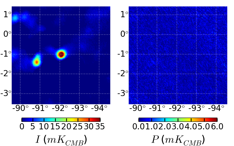
(a) “Reference”

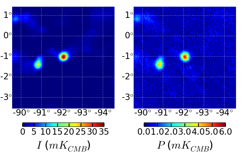
(b) “Non-Linear”

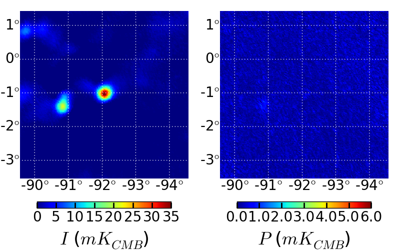
(c) “ICP removed”

Figure 8: Simulations of RCW38 maps in intensity and polarization power $P$ for three simulated datasets: “reference” (left), non-linear (middle), “ICP removed” (right). The maps shown in Galactic coordinates co-add 216 detectors. The polarization orientation is reconstructed in the instrument frame.

CMB Stacked Spots in the Instrument Frame

Figure 9 shows the CMB stacked spots constructed from the three simulated datasets. The polarization orientation is co-added in the instrument frame. The non-linear time-streams (middle) produce a coupling fraction of 17% that is visible in the center of the $P$ stacked spots. The coupling coefficients produced by the non-linear simulation are in agreement with those measured in EBEX data (see linear slope in Table 1). In the ICP removed dataset, 95% of the ICP has been removed.

CMB Stacked Spots in the Sky Frame

We plot in Figure 10 the stacked spots in the sky frame for the three simulated datasets. When stacking CMB spots in the sky frame, E-modes are apparent as rings of polarization power surrounding the cold and hot $I$ spots. For this analysis we used noiseless simulations because adding the EBEX2013 level of noise would have entirely obscured the polarization structure apparent in Figure 10 (a). The 17% ICP completely obscures the E-modes in the non-linear dataset. In the ICP removed dataset, 99% of the ICP is removed and the standard deviation between the input and recovered E-modes is 0.01 uK.

(a) “Reference”

(b) “Non-Linear”

(c) “ICP removed”

Figure 9: Simulations of CMB stacked spots in intensity and polarization power $P$ for three simulated datasets: “reference” (left), “non-linear” (middle), “ICP removed” (right). The polarization orientation is reconstructed in the instrument frame. 95% of the 17% ICP is removed in the cleaned dataset (right).

(a) “Reference”

(b) “Non-Linear”

(c) “ICP removed”

Figure 10: Simulations of CMB stacked spots in intensity and polarization power $P$ for three simulated datasets: “reference” (left), “non-linear” (middle), “ICP removed” (right). The polarization orientation is reconstructed in the sky frame. Note that the colorscale in polarization is different from the previous stacked spots presented, and that these simulations are noiseless. These noiseless maps were produced early in the analysis and have a larger pixel size than other stacked spots presented in the paper.

7.2 EBEX2013

The ICP removal procedure is applied to EBEX2013 data, for both 150 and 250 GHz detectors. The Galaxy is used to measure coupling coefficients, which are then used to produce time-streams with the ICP removed. We present RCW38 maps generated before and after removal in Figure 11, and CMB stacked spots in Figure 12. Table 4 summarizes the ICP Pearson correlation and coupling coefficients in each frequency band before and after removal of the excess polarization. For RCW38, 67% (98%) of the ICP is removed at 150 (250) GHz. In the stacked spots, 81% (92%) of the excess polarization is removed.

RCW 38 CMB Stacked Spots Correlation Linear Correlation Linear Coefficient Slope (%) Coefficient Slope (%) EBEX 150 GHz 0.8 11 0.8 8 EBEX 150 GHz with ICP removed 0.4 3 0.2 2 EBEX 250 GHz 0.8 12 0.6 16 EBEX 250 GHz with ICP removed 0.5 0 0.1 1

Table 4: Pearson correlation and linear slope (corresponding to $A^{\prime}_{4}$ averaged over detectors) between $I$ and $P$ after the excess polarization removal. For ease of comparison, the pre-removal numbers are copied over from Table 1.

(a) 150 GHz

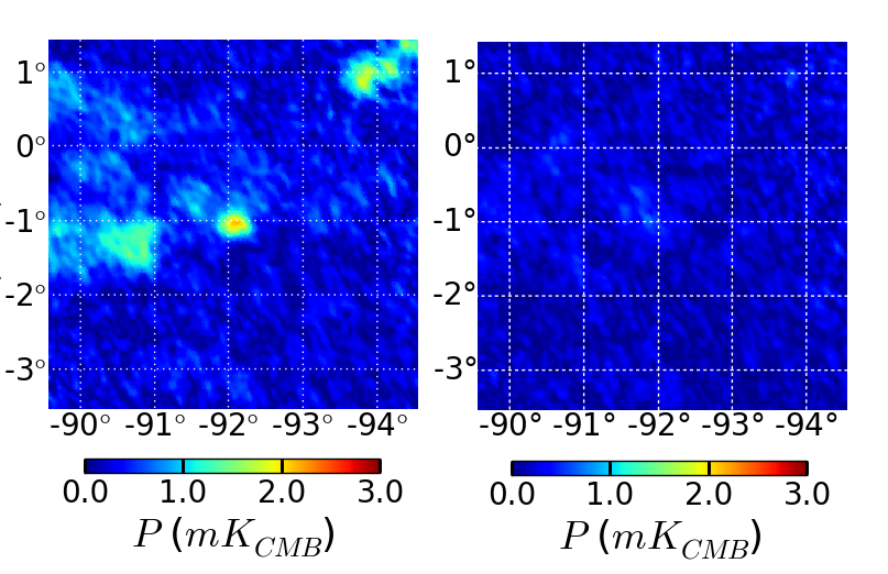
(b) 250 GHz

Figure 11: Comparison of RCW38 maps in polarization power $P$ before (left) and after (right) ICP removal for 150 GHz (Figure (a)) and 250 GHz (Figure (b)) EBEX detectors. The polarization orientation is reconstructed in the instrument frame.

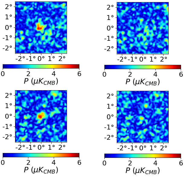
(a) 150 GHz

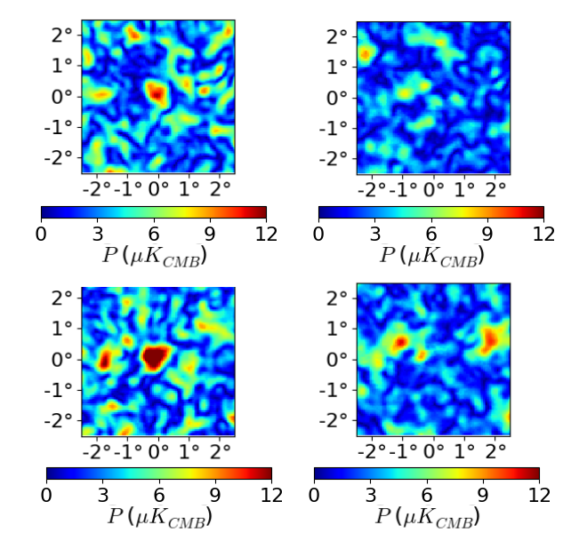
(b) 250 GHz

Figure 12: Comparison of CMB stacked spots in polarization power $P$ before and after ICP removal for 150 GHz (left four) and 250 GHz (right four) EBEX detectors. Within each frequency band, the maps are shown before (left) and after (right) excess polarization removal. Hot and cold spot are shown on the top and bottom panels, respectively. The polarization orientation is reconstructed in the instrument frame.

7.3 Discussion and Summary

Continuously rotating HWP are increasingly used in CMB instruments because they reduce ICP originating from detector differencing and because they mitigate low frequency noise enabling observations on large angular scales, which are otherwise limited by atmospheric turbulence. Considering ICP alone, the HWP should be the first element in the optical path, in order to modulate only incident polarized sky signals. With the EBEX instrument, which had a 1.5 m entrance aperture, it was not practical for the HWP to be the first element in the optical path. We placed it behind the field lens, heat-sunk to a temperature of 4 K, to reduce optical load on the detectors. We anticipated $\acs{ICP}^{IP}$ of up to 2.7%. The data showed an ICP larger than 10%. We found that the relatively large HWPSS induced non-linear detector response, which in turn caused significant conversion of intensity signals to polarization, ICP^NL.

We developed and applied an ICP removal method to the EBEX2013 data, using the Galaxy to measure coupling parameters and assessing the quality of the removal on RCW38 maps and CMB stacked spots. We showed that for the EBEX2013 data 81 (92) % of the ICP was removed from the CMB at 150 (250) GHz using this technique. The removal of the ICP performs better at 250 GHz compared to 150 GHz. We think this is due to the 150 GHz detectors having an elliptical beam that is not taken into account during calibration or when using a reference map to measure the coupling parameters and subtract the excess polarization (only a symmetrical fit to the beam is used). This would also explain why the ICP removal works better on the CMB stacked spots smoothed to 0.5$\mathrm{\SIUnitSymbolDegree}$ compared to RCW38 maps which vary on smaller scales. We note that the CMB stacked spots are a good test of the quality of the removal as it uses a separate dataset (CMB) than is used to compute the coupling parameters (Galaxy).

The method we presented removes ICP regardless of its source. However, if the detectors have a non-linear response, other effects are present in addition to ICP^NL, such as attenuation of $I^{sky}$ and $P^{sky}$, as demonstrated in the simulations by comparing $I$ in the reference and non-linear plots in Figure 8 and 9. These effects are not corrected by the ICP removal method. Our method, as is the method presented by Takakura et al. (2017), does not correct the non-linearity of the detectors and does not correct the distortion induced due to the non-linearity upon incident sky $Q$ and $U$ Stokes signals. The level of these distortion needs to be assessed separately, particularly for experiments targeting higher precision polarimetry. Alternatively, non-linearity should be avoided by reducing the range of incoming signals (in particular the HWPSS), or by using detectors with operating parameters that ensure linear response over a larger dynamic range of incident signals.

Appendix A Coordinates

Throughout the paper we alternate between reconstructing the polarization in a frame rotation fixed with the Galactic coordinate system and a frame rotation fixed with the instrument. This is useful to separate polarization originating from the sky against polarization originating from the instrument, as each adds up coherently only in their respective frame orientations. When pointing in a given direction, the two frames are rotated from each other by the instrument Galactic roll angle $\psi_{t}$. The $\Phi_{t}$ offset angle from Equation 1 can be broken up into:

$$\Phi_{t}=\Phi^{\prime}+2\psi_{t}$$ (A1)

where $\Phi^{\prime}$ is now constant. For simplicity we do not write out $\Phi^{\prime}$ or the modulation efficiency $\epsilon$ in the paper. For the celestial reference frame we adopt the Wilkinson Microwave Anisotropy Probe (WMAP) conventions (Komatsu et al., 2011): the polarization that is parallel to the Galactic meridian is $Q$ $>$ 0 and $U$ = 0, and the polarization that is rotated by 45$\mathrm{\SIUnitSymbolDegree}$ from east to west (clockwise, as seen by an observer on Earth looking up at the sky) has $Q$ = 0 and $U$ $>$ 0. In the instrument frame, positive $Q$ corresponds to linear polarization along the x-axis and positive $U$ corresponds to polarization 45$\mathrm{\SIUnitSymbolDegree}$ between the +x and +y directions. The axes are labelled in Figure 1.

Appendix B Effect of a Di-attenuator on Unpolarized Light

The field lens acts as a di-attenuator and polarizes light because of differential transmittance between in plane and out of plane incidence. The Mueller matrix of a di-attenuator with in-plane direction forming an angle $\delta$ with the x-axis is:

$$G(\delta)=\frac{1}{2}\,R(-\delta)\left(\begin{array}[]{cccc}\eta&\varepsilon&0&0\\ \varepsilon&\eta&0&0\\ 0&0&\sqrt{\eta^{2}-\varepsilon^{2}}&0\\ 0&0&0&\sqrt{\eta^{2}-\varepsilon^{2}}\end{array}\right)R(\delta)$$ (B2)

where $R(\delta)$ is the Mueller rotation matrix, $\eta$ $\sim$ $2$ is the sum of the transmittances along the two perpendicular axis and $\varepsilon$ $\sim$ $0$ is the difference between the transmittances of the two axis. The amount of IP is characterized by $\varepsilon$, that we name $\varepsilon^{IP}$ in the text. Note that $\varepsilon^{IP}$ increases as the angle of incident light increases, producing more IP at the edge of the field lens than in the center. To calculate the effect of the field lens on incoming unpolarized light $I$, the instrument Mueller matrix is modified to include $G(\delta)$:

$$M_{instr}=M_{lp}M_{hwp}(\gamma_{t})\,G(\delta)$$ (B3)

Using Equations B3 and 8, this results in the following detector time-stream:

$$\vec{S}^{IP}_{t} =M_{instr}\left(\begin{array}[]{c}I^{instr}\\ 0\\ 0\\ 0\end{array}\right)$$ (B5)

$$D^{IP}_{t} =I^{IP}_{t}$$

$$=\frac{1}{2}I^{instr}\,(\eta+\varepsilon^{IP}\cos(4\gamma_{t}-2\delta))$$ (B6)

Appendix C Non-Linear Response of a TES bolometer

In the EBEX detector readout (Aubin, 2012; MacDermid, 2014), the change in current $i$ coming from a change in power $\delta P$ incident on the detector can be expanded into a series about the equilibrium point $i_{0}$:

$$i(\delta P)-i_{0} =\diff{i}{P}\delta P+\frac{1}{2}\diff{{}^{2}i}{P^{2}}\delta P^{2}+..$$

$$=a\,\delta P+b\,\delta P^{2}+...$$ (C1)

We limit our non-linearity model to second order terms and ignore time-constant effects. Let us show that $a$ and $b$ have opposite signs, which will justify our subsequent choice of non-linear function. The current $i$ is a function of the bias voltage $V$ and the detector resistance $R(T)$:

$$i=\frac{V}{R(T)}$$ (C2)

such that the current $i$ can be expressed as:

$$i(\delta P)-i_{0} =-\frac{V}{R_{0}^{2}}\diff{R}{T}\diff{T}{P}\,\delta P+\big{(}2\frac{V}{R_{0}^{3}}\Big{[}\diff{R}{T}\Big{]}^{2}-\frac{V}{R_{0}^{2}}\diff{{}^{2}R}{T^{2}}\big{)}\Big{[}\diff{T}{P}\Big{]}^{2}\,\delta P^{2}$$ (C3)

$$=a\,\delta P+b\,\delta P^{2}$$ (C4)

where $R_{0}$ is the detector resistance at the equilibrium point. We assume the thermal response to incoming power is linear. $a$ is negative because $R$ increases with increasing temperature $T$, and $b$ is positive because in TES detectors, $\diff{{}^{2}R}{T^{2}}$ is negative high in the transition (during the EBEX flight, $R_{0}$ was at 65% to 85% of its over-biased resistance $R_{N}$). Dividing by the responsivity $a$, we can write the non-linear detector response as:

$$f^{NL}(\delta P)=\delta P-K\delta P^{2}$$ (C5)

where $K>0$.

References

- Araujo (2017) Araujo, D. 2017, PhD thesis, Columbia University
- Aubin (2012) Aubin, F. 2012, PhD thesis, McGill University
- Aubin et al. (2016) Aubin, F., Aboobaker, A. M., Ade, P., et al. 2016, in Proceedings of the 14th Marcel Grossman Conference
- BICEP2 Collaboration et al. (2015) BICEP2 Collaboration, Ade, P. A. R., Aikin, R. W., et al. 2015, ApJ, 814, arXiv:1502.00608
- Didier (2016) Didier, J. 2016, PhD thesis, Columbia University
- Essinger-Hileman et al. (2016) Essinger-Hileman, T., Kusaka, A., Appel, J. W., Choi, S. K., et al. 2016, Review of Scientific Instruments, 87, arXiv:1601.05901
- Górski et al. (2005) Górski, K. M., Hivon, E., Banday, A. J., et al. 2005, ApJ, 622, 759
- Johnson et al. (2007) Johnson, B., Collins, J., Abroe, M., et al. 2007, ApJ, 665, 42
- Komatsu et al. (2011) Komatsu, E., Smith, K. M., Dunkley, J., et al. 2011, ApJS, 192, 18
- Kusaka et al. (2014) Kusaka, A., Essinger-Hileman, T., Appel, J. W., Gallardo, P., et al. 2014, Review of Scientific Instruments, 85, arXiv:1310.3711v2
- MacDermid (2014) MacDermid, K. 2014, PhD thesis, McGill University
- Matsumura (2006) Matsumura, T. 2006, PhD thesis, University Of Minnesota
- Pancharatnam (1955) Pancharatnam, S. 1955, Proceedings of the Indian Academy of Sciences, Section A, 41, 137
- Shimon et al. (2008) Shimon, M., Keating, B., Ponthieu, N., & Hivon, E. 2008, Phys.Rev.D., 77, 083003
- Strozzi & McDonald (2000) Strozzi, D. J., & McDonald, K. T. 2000, Polarization Dependence of Emissivity, , , arXiv:physics/0005024
- Takakura et al. (2017) Takakura, S., Aguilar, M., Akiba, Y., Arnold, K., et al. 2017, J. Cosmology Astropart. Phys, arXiv:1702.07111
- The EBEX Collaboration (2017a) The EBEX Collaboration. 2017a, ApJS, in preparation
- The EBEX Collaboration (2017b) —. 2017b, ApJS, accepted, arXiv:1702.07020
- The EBEX Collaboration (2017c) —. 2017c, ApJS, accepted, arXiv:1703.03847