On causality violation on a Kerr-de Sitter spacetime

Abstract

The causal properties of the family of Kerr-de Sitter spacetimes are analyzed and compared to those of the Kerr family. First, an inextendible Kerr-de Sitter spacetime is obtained by joining together Carter’s blocks, i.e. suitable four dimensional spacetime regions contained within Killing horizons or within a Killing horizon and an asymptotic de Sitter region. Based on this property, and leaving aside topological identifications, we show that the causal properties of a Kerr-de Sitter spacetime are determined by the causal properties of the individual Carter’s blocks viewed as spacetimes in their own right. We show that any Carter’s block is stably causal except for the blocks that contain the ring singularity. The latter are vicious sets, i.e.  any two events within such block can be connected by a future (respectively past) directed timelike curve. This behavior is identical to the causal behavior of the Boyer-Lindquist blocks that contain the Kerr ring singularity. These blocks are also vicious as demonstrated long ago by Carter. On the other hand, while for the case of a naked Kerr singularity the entire spacetime is vicious and thus closed timelike curves pass through any event including events in the asymptotic region, for the case of a Kerr-de Sitter spacetime the cosmological horizons protect the asymptotic de Sitter region from a-causal influences. In that regard, a positive cosmological constant appears to improve the causal behavior of the underlying spacetime.

I Introduction

In this paper, we discuss causality violations taking place within the family of Kerr-de Sitter spacetimes. Since the specification of the regions where these violations take place requires an understanding of the global structure of the underlying spacetime, in this paper we also review some of the global properties of the Kerr-de Sitter spacetimes. In that respect, we start from a Kerr-de Sitter metric written in Boyer-Lindquist coordinates and show that this, in general geodesically incomplete, spacetime referred to as a Carter’s block, can be extended through Killing horizons to generate an inextendible Kerr-de Sitter spacetime. This property permits us to introduce Carter-Penrose like diagrams and present evidence suggesting that these diagrams are similar to the diagrams describing the two dimensional rotation axis of a Kerr-de Sitter spacetime. Furthermore, we conclude that the causality properties of any four dimensional Kerr-de Sitter spacetime are determined by the causality properties of the individual Carter’s blocks. We prove that any Carter’s block is stably causal except for the blocks that contain the ring singularity. These latter blocks are vicious sets in the sense defined by Carter Car3 : Any two events within a block that contains the ring singularity can be connected by a future (resp. past) directed timelike curve. This highly counterintuitive property was shown by Carter to hold for any Boyer- Lindquist block that contains the ring singularity in a Kerr (or a Kerr-Newman) spacetime and in this work we show that the same property holds for the blocks that contain the ring singularity in any Kerr-de Sitter spacetime.

In order to prove this property, at first we show that for any Kerr-de Sitter spacetime the block that contains the ring singularity also contains a non empty Carter’s time machine (CTM), i.e. a spacetime region where the axial Killing vector field becomes temporal. Using this CTM, we prove that any two events $(I,F)$ in this block can be joined by a timelike future (resp. past) pointing curve. For this, we construct three future pointing timelike segments with the following characteristics: the first one originates in the event $I$ and terminates in an event on the equatorial plane $\vartheta=\frac{\pi}{2}$ of the CTM. The second segment is also timelike and future pointing and starts from the event where the first segment ends and proceeds with the value of the Boyer Lindquist coordinate $t$ decreasing while it remains on the $\vartheta=\frac{\pi}{2}$ plane of the CTM. The final segment, is again timelike and future pointing and starts from the event where the second segment terminates and ends at the event $F$. In section $V$ we give the explicit representation of these segments and discuss their properties.

The proof of the vicious nature of any Carter’s block that contains the ring singularity illustrates the role of the CTM in destroying any notion of causality. It is worth mentioning here that although Carter in Car3 strongly emphasizes the negative impact that a non empty CTM has upon causality, nevertheless in the current literature and standard textbooks it seems that the vicious nature of the blocks that contain the ring singularity is overlooked. One gets the impression that causality violation in the Kerr-Newman family takes place only within the tiny spacetime region that finds itself within the CTM, while the vicious nature of the entire block that contains the ring singularity is rarely mentioned. This work shows (and emphasizes) that, either for the case of Kerr or Kerr-de Sitter, causality is violated within the entire block that contains the ring singularity.

The structure of the present paper is as follows: in the next section, we introduce the family of Kerr-de Sitter metrics. The subsequent section contains a brief construction of the maximal analytical extension of the rotation axis of a Kerr-de Sitter spacetime, while section $IV$ discusses the global structure of a four dimensional Kerr-de Sitter. In section $V$, we prove three propositions describing the causal properties of a Kerr-de Sitter spacetime. We finish the paper with a discussion of some open problems while in an Appendix the reader is reminded of a few basic notions of causality theory.

II Some Properties of the Kerr-de Sitter Spacetimes

The family of the Kerr-de Sitter spacetimes was discovered long ago by Carter Car1 ,Car2 . In a local set of Boyer-Lindquist coordinates $(t,\varphi,r,\vartheta)$, the Kerr-de Sitter metric $g$ takes the form:

$$g=-\frac{\Delta(r)}{I^{2}\rho^{2}}[dt-a\sin^{2}{\theta}d\varphi]^{2}+\frac{\hat{\Delta}(\vartheta)\sin^{2}\vartheta}{I^{2}\rho^{2}}[adt-(r^{2}+a^{2})d\varphi]^{2}+\frac{\rho^{2}}{\Delta(r)}dr^{2}+\frac{\rho^{2}}{\hat{\Delta}(\vartheta)}d\vartheta^{2}$$ (1)

$$\rho^{2}:=r^{2}+a^{2}\cos^{2}\vartheta,\quad\Delta(r):=-\frac{1}{3}\Lambda r^{2}(r^{2}+a^{2})+r^{2}-2mr+a^{2},\quad{\hat{\Delta}}(\vartheta):=1+\frac{1}{3}\Lambda a^{2}\cos^{2}\vartheta,\quad I:=1+\frac{1}{3}\Lambda a^{2},$$

where above and hereafter $\Lambda>0$ stands for the cosmological constant, $m$ is the mass parameter and $a$ is a rotation parameter. The $t$-coordinate takes its values over the real line, the angular coordinates $(\vartheta,\varphi)$ vary in the familiar range, while $r$ is restricted to suitable open sets of the real line that are specified further below. The fields $\xi_{t}=\frac{\partial}{\partial t}$ and $\xi_{\varphi}=\frac{\partial}{\partial\varphi}$ are commuting Killing fields and the zeros of $\xi_{\varphi}$ define the rotation axis.
From (1), it follows that the non vanishing covariant components $g_{\mu\nu}$ of $g$ are:

$$g_{tt}=-\frac{{\Delta({r})}-{{\hat{\Delta}}}({\vartheta})a^{2}sin^{2}\vartheta}{I^{2}\rho^{2}},~{}~{}~{}g_{t\varphi}=\frac{\Delta(r)-{\hat{\Delta}}({\vartheta})(r^{2}+a^{2})}{I^{2}\rho^{2}}asin^{2}\vartheta,$$ (2)

$$g_{\varphi\varphi}=\frac{{\hat{\Delta}}({\vartheta})(r^{2}+a^{2})^{2}-\Delta(r)a^{2}sin^{2}\vartheta}{I^{2}\rho^{2}}sin^{2}\vartheta,~{}~{}~{}~{}~{}g_{rr}=\frac{\rho^{2}}{\Delta(r)},\quad\quad g_{\vartheta\vartheta}=\frac{\rho^{2}}{\hat{\Delta}(\vartheta)}$$ (3)

while the non vanishing contravariant components $g^{\mu\nu}$ are:

$$g^{tt}=-\frac{I^{2}[{\hat{\Delta}(\vartheta)}(r^{2}+a^{2})^{2}-{\Delta(r)}a^{2}sin^{2}\vartheta]}{\rho^{2}{\hat{\Delta}(\vartheta)}{\Delta(r)}},~{}~{}~{}~{}~{}g^{t\varphi}=\frac{I^{2}a[{\Delta(r)}-{\hat{\Delta}(\vartheta)}(r^{2}+a^{2})]}{\rho^{2}{\hat{\Delta}(\vartheta)}{\Delta(r)}}$$ (4)

$$g^{\varphi\varphi}=\frac{I^{2}[{\Delta(r)}-{\hat{\Delta}(\vartheta)}a^{2}sin^{2}\vartheta]}{\rho^{2}sin^{2}\vartheta{\hat{\Delta}(\vartheta)}{\Delta(r)}},~{}~{}~{}~{}~{}g^{rr}=\frac{\Delta{(r)}}{\rho^{2}},\quad g^{\vartheta\vartheta}=\frac{\hat{\Delta}{(\vartheta)}}{\rho^{2}}.$$ (5)

Algebraic manipulations of the scalar invariants show that the curvature of (1) becomes unbounded as $\rho\to 0$, i.e. as the ring ($r=0$, $\vartheta=\frac{\pi}{2}$) is approached. Besides this ring-like curvature singularity, singularities in the components of $g$ in (1) occur along the rotation axis, i.e. at $\sin\vartheta=0$, and these singularities can be removed by introducing local coordinates or introducing generalized Kerr-Schild coordinates. Singularities in the components of (1) also occur at the roots of the quartic equation $\Delta(r)=0$ and these are also coordinate singularities. Depending upon the values of $(\Lambda,m,a),$ the quartic equation $\Delta(r)=0$ may admit up to four distinct real roots exhibiting one of the following arrangements (see for instance the discussion in LakZan ):

a) all four roots are real and distinct, arranged according to: $r_{1}<0<r_{2}<r_{3}<r_{4}$,

b) all roots are real but $r_{2}$ is doubly degenerate, i.e. $r_{1}<0<r_{2}=r_{3}<r_{4}$,

c) all roots are real but $r_{4}$ is doubly degenerate, i.e. $r_{1}<0<r_{2}<r_{3}=r_{4}$,

d) the three positive roots coincide, i.e. $r_{1}<0<r_{2}=r_{3}=r_{4}$,

e) the equation $\Delta(r)=0$ admits a pair of complex conjugate roots and a pair of real roots: $r_{1}<0<r_{2}.$

Clearly, any open interval $(r_{i},r_{i+1})$ where $r_{i}$, $r_{i+1}$ are consecutive roots of $\Delta(r)=0$, combined with the metric $g$ in (1) defines a (geodesically incomplete) spacetime covered by a single Boyer-Lindquist chart $(t,r,\vartheta,\varphi)$. Any one of these spacetimes is denoted hereafter by $(T_{(r_{i},r_{i+1})},g)$ and is referred as a Carter’s block. The blocks $(T_{(r_{4},\infty)},g)$ and $(T_{(-\infty,r_{1})},g)$ define the two asymptotic blocks, while $(T_{(r_{1},r_{2})},g)$ stands for the block that contains the ring singularity. As we shall see in the next sections, Carter’s blocks can be glued together along null hypersurfaces that are actually Killing horizons and thus these blocks determine the global structure of a Kerr-de Sitter spacetime.

We finish this section by introducing a few auxiliary fields that will be helpful later on. The canonical vector fields:

$$V=(r^{2}+a^{2})\frac{\partial}{\partial t}+a\frac{\partial}{\partial\varphi},\quad W=\frac{\partial}{\partial\varphi}+a\sin^{2}\vartheta\frac{\partial}{\partial t}$$ (6)

are well defined on any Carter’s block and satisfy:

$$g(V,V)=-\frac{\rho^{2}\Delta(r)}{I^{2}},\quad g(W,W)=\frac{\rho^{2}\sin^{2}\vartheta{\hat{\Delta}}(\vartheta)}{I^{2}},\quad g(V,W)=0.$$ (7)

These fields and the coordinate basis fields in (1) obey:

$$g(V,\frac{\partial}{\partial r})=g(V,\frac{\partial}{\partial\vartheta})=g(W,\frac{\partial}{\partial r})=g(W,\frac{\partial}{\partial\vartheta})=0$$

$$g(\frac{\partial}{\partial r},\frac{\partial}{\partial r})=\frac{\rho^{2}}{\Delta(r)},\quad g(\frac{\partial}{\partial\vartheta},\frac{\partial}{\partial\vartheta})=\frac{\rho^{2}}{{\hat{\Delta}}(\vartheta)}.$$ (8)

while the gradient fields,

$$L_{t}=\nabla^{a}t\frac{\partial}{\partial x^{a}},\quad L_{r}=\nabla^{a}r\frac{\partial}{\partial x^{a}},$$ (9)

satisfy

$$g(L_{t},L_{t})=g^{tt}=-\frac{I^{2}[{\hat{\Delta}(\vartheta)}(r^{2}+a^{2})^{2}-{\Delta(r)}a^{2}\sin^{2}\vartheta]}{\rho^{2}{\hat{\Delta}(\vartheta)}{\Delta(r)}},\quad\quad g(L_{r},L_{r})=\frac{\Delta(r)}{\rho^{2}}.$$ (10)

Formulas $(\ref{Eq:CF}-\ref{Eq:MTF})$ will be used further ahead.

III On the Maximal analytical extension of the rotation axis

The discussion in the previous section suggests that the Carter’s blocks should be viewed as open submanifolds in a larger Kerr-de Sitter manifold and the issue we address in the next sections concerns the structure of this larger Kerr-de Sitter manifold.

We recall that Carter, in ref.Car3 , obtained the maximal analytical extension of the Kerr metric guided by the maximal analytical extension of the two dimensional rotation axis of a Kerr spacetime combined with the behavior of causal geodesics on a Kerr background. Interestingly, below, we show that the maximal analytical extension of the rotation axis of a Kerr-de Sitter offers clues regarding the global structure of the four dimensional Kerr-de Sitter spacetime. In order to make this connection clear, at first we briefly discuss the maximal analytical extension of the rotation axis of a Kerr-de Sitter spacetime.

The rotation axis of a Kerr-de Sitter spacetime is identified as a two dimensional closed, totally geodesic submanifold consisting of the zeros of the axial Killing field (for a definition and properties of totally geodesic submanifolds see ref.Neil , page $48$). Since the Boyer-Lindquist coordinates in (1) do not cover this submanifold, we introduce new local coordinates $(x,y)$ via $x=\sin\vartheta\cos\varphi$ and $y=\cos\vartheta\sin\varphi$ so that $(t,r,x=y=0)$ defines the rotation axis. Relative to these $(t,r,x,y)$ coordinates the induced metric $g_{in}$ on the axis takes the form (for details see FT1 ):

$$g_{in}=-f(r)dt^{2}+\frac{dr^{2}}{f(r)},\quad f(r)=\frac{\Delta(r)}{r^{2}+a^{2}},\quad(t,r)\in R\times(r_{i},r_{i+1})$$ (11)

where a factor of $I=1+\frac{1}{3}\Lambda a^{2}$ has been absorbed in a redefinition of the Killing time. Whenever $\Delta(r)=0$ admits four distinct real roots $r_{1}<0<r_{2}<r_{3}<r_{4}$, then (11) defines five two dimensional spacetimes representing disconnected components of the rotation axis. These five two dimensional spacetimes can be glued together yielding eventually the maximal analytical extension of the rotation axis.

Figure 1: The figure on the left represents the Carter-Penrose diagram for the two dimensional ingoing spacetime $(IEF,g_{i})$ introduced in the main text with the embedding of the five two dimensional spacetimes included in (11) indicated. Ingoing null geodesics extend from $\infty$ up to $-\infty$ and thus are complete. By standard conventions these geodesics are considered as future pointing and thus time-orient $(IEF,g_{i})$. Incomplete outgoing null geodesics are also indicated. The figure on the right represents the Carter-Penrose diagram for the two dimensional outgoing spacetime $(OEF,g_{o})$. Here, outgoing null geodesics are complete and future pointing running from $-\infty$ to $\infty$. Incomplete ingoing ones are also shown.
As discussed in section IV, these diagrams also schematically represent the four dimensional ingoing Kerr-de Sitter $(IKS,\hat{g}_{i})$ (left figure) and the four dimensional outgoing Kerr-de Sitter $(OKS,\hat{g}_{o})$ (right figure). In such an interpretation, the blocks are four dimensional Carter’s blocks, the null lines marked by $r_{1},r_{2}$, etc., represent Killing horizons. Principal ingoing and outgoing null geodesics are also indicated.

In order to carry out this gluing processes, we start from $(M_{1},g_{1})$ (see footnote (7) for the definition of $(M_{1},g_{1})$) and introduce ingoing Eddington-Finkelstein coordinates $(v,\hat{r})$ via

$$dv=dt+\frac{dr}{f(r)},~{}d\hat{r}=dr,\quad t\in(-\infty,\infty),~{}r\in(r_{1},r_{2}).$$

so that

$$g_{1}=-f(r)dv^{2}+2dvdr,\quad(v,r)\in R\times(r_{1},r_{2})$$ (12)

where above and whenever there is no danger of confusion we write $r$ instead of $\hat{r}$. Since this $g_{1}$ is regular over the roots of $\Delta(r)=0$, using the function $f(r)$ in (11), we extend $(M_{1},g_{1})$ by allowing the coordinates $(v,r)$ to run over $R\times R$ and refer to this extended spacetime as a two dimensional ingoing Eddington-Finkelstein, denoted by $(IEF,g_{i})$. The extended metric $g_{i}$ is defined by:

$$g_{i}=-f(r)dv^{2}+2dudr,\quad(v,r)\in R\times R.$$

This $(IEF,g_{i})$ has the property that the family of cutves $v=const$ and $-r\in(-\infty,\infty)$ represents the ingoing, complete family of radial null geodesics with $-r\in(-\infty,\infty)$ acting as an affine parameter. This null geodesic congruence has $L=-\frac{\partial}{\partial r}$ as the tangent null vector field and it is customary to consider $L$ as being future pointing and thus providing the global time orientation on $(IEF,g_{i})$.

It is not difficult to verify that any of the five two dimensional spacetimes included in (11), can be isometrically embedded as open submanifolds within $(IEF,g_{i})$. For instance starting from $(M_{2},g_{2})$, we introduce ingoing Eddington-Finkelstein coordinates $(\hat{v},\hat{r})$ via

$$d\hat{v}=dt+\frac{dr}{|f(r)|},~{}d\hat{r}=dr,\quad t\in(-\infty,\infty),~{}r\in(r_{2},r_{3})$$

so that $g_{2}$ takes the form

$$g_{2}={|f(r)|}dt^{2}-\frac{1}{{|f(r)|}}dr^{2}={|f(r)|}d{\hat{v}}^{2}-2d{\hat{v}}d\hat{r},\quad(\hat{v},\hat{r})\in R\times(r_{2},r_{3})$$ (13)

and subsequently embed this $(M_{2},g_{2})$ within $(IEF,g_{i})$ via the map:

$$\Phi:M_{2}\to IEF:(\hat{v},\hat{r})\to\Phi(\hat{v},\hat{r})=(v(\hat{v},\hat{r}),r(\hat{v},\hat{r}))=(-\hat{v},\hat{r}),$$ (14)

which is a smooth isometry of $M_{2}$ onto $\Phi(M_{2}).$ For the case of $(M_{3},g_{3})$ the isometry $\Phi$ has the same form as the one described in (14) with the only exception that $-\hat{v}$ is replaced by $\hat{v}$ and so on. In view of these embeddings, the conformal Carter-Penrose diagram for $(IEF,g_{i})$ has the form shown in the left diagram of Fig.1.

We now shift our attention to the outgoing family of null geodesics and begin considering again $(M_{1},g_{1})$, but now introduce outgoing Eddington-Finkelstein coordinates $(u,\hat{r})$ via:

$$du=dt-\frac{dr}{f(r)},~{}d\hat{r}=dr,\quad t\in(-\infty,\infty),~{}r\in(r_{1},r_{2})$$

so that $g_{1}$ takes the form:

$$g_{1}=-f(r)du^{2}-2dudr,\quad(u,r)\in R\times(r_{1},r_{2}).$$ (15)

Through the same arguments that lead us to $(IEF,g_{i})$, we now introduce the outgoing Eddington-Finkelstein spacetime $(OEF,g_{o})$ with

$$g_{o}=-f(r)du^{2}-2dudr,\quad(u,r)\in R\times R.$$ (16)

Clearly this $g_{o}$ is regular over the entire domain of the radial coordinate $r$ and for this $(OEF,g_{o})$, the outgoing family of null geodesics is described by $u=const$, $r\in(-\infty,\infty)$ with $r$ acting as an affine parameter. This family has $L=\frac{\partial}{\partial r}$ as the tangent null vector field taken to be future pointing and thus defines the global time orientation on $(OEF,g_{o})$. The remaining two dimensional spacetimes included in (11) can be isometrically embedded as open submanifolds within $(OEF,g_{o})$ so that the resulting Carter-Penrose diagram is the right diagram shown in Fig.1.

The final step leading to an extension of the rotation axis of a Kerr-de Sitter consists of gluing together the two diagrams shown in Fig.1 in such a manner that the radial ingoing and outgoing null geodesics become simultaneously complete. Here, some care is required so that the gluing procedure yields an extended spacetime admitting a consistent time orientation. One way to achieve this is to start from a copy of an ingoing Eddington-Finkelstein spacetime $(IEF,g_{i})$ shown in Fig.1, and on a specific block introduce simultaneously outgoing Eddington-Finkelstein coordinates. Subsequently extend that block in the future direction by appending a part of the outgoing Eddington-Finkelstein spacetime and making sure that the resulting spacetime admits a consistent time orientation. Leaving details aside, the resulting Carter-Penrose diagram is shown in Fig.2 and this diagram is also introduced in refs.GibHaw1 ,Car2 .

To finish this section, we mention that the use of Eddington-Finkelstein coordinates as the means to construct the Carter-Penrose diagram shown in Fig.2, does not cover the vertex where the four horizons meet. However, this deficiency can be removed by introducing Kruskal coordinates which are well defined provided the roots of $f(r)=0$ are all simple roots. We do not enter into these details here (they are discussed in F ,FT2 ), but we only mention that the extension shown in Fig.2 is a maximal analytical extension of the rotation axis. Maximality follows by verifying that any causal geodesic on this two dimensional spacetime is actually complete while the analytical nature of the extension follows from the analyticity of the function $f(r)$ in (11).

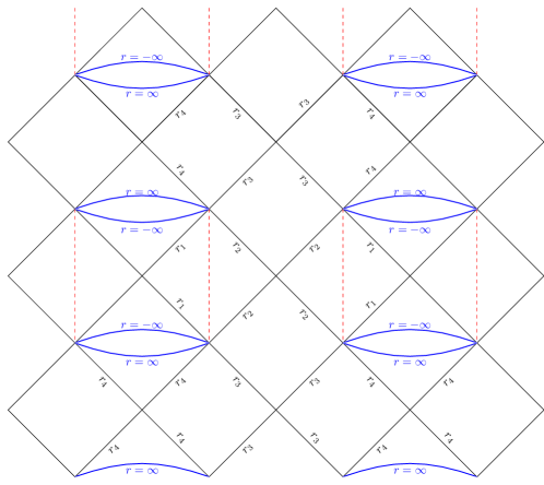
Figure 2: The Carter-Penrose diagram for the two dimensional rotation axis of a Kerr-de Sitter spacetime (see also GibHaw1 ,Car2 ). As we discussed in section IV, this diagram can represent schematically the structure of a four dimensional Kerr-de Sitter spacetime. When interpreted in that way, the dashed lines (red in the colored version of the figure) remind the reader of the location of the ring singularity, while the curved lines (blue in the colored version) representing $r\to\pm{\infty}$ signify that these regions are distinct. For this spacetime, the causality violating regions are the union of the blocks containing the ring singularity. If the topology of the spacetime is altered by identifying, for instance, asymptotic regions, then the causality violating regions are altered as well.

IV On the maximal analytical extension of a Kerr-de Sitter Spacetime

Even though the construction of the maximal analytical extension of the two dimensional rotation axis of a Kerr-de Sitter spacetime was a relatively easy task to accomplish, the construction of the maximal analytical extension of a four dimensional Carter’s block is not that straightforward a task. An extension of a Carter’s block could be obtained by following the same method as the one employed by Carter in extending the Kerr family of metrics (for details see Car3 ). However, we should be aware that in this approach, in order to address the maximality property of the extended spacetime, the behavior of causal geodesics on the extended background is required. Although causal geodesics on a Kerr-de Sitter have been the subject of many investigations, these targeted particular families of geodesics, such as the family of equatorial Stuc3 , polar Tso , spherical The or geodesics confined on a particular Carter’s block Laz . In a recent work FT1 , the completeness property of geodesics defined on an arbitrary Carter’s block has been addressed and evidence was found to support the view that “almost all causal geodesics“ defined initially on a Carter’s block can be extended as geodesics through Killing horizons so they become complete except for those ones that hit the ring singularity. Due to this incomplete understanding of the behavior of causal geodesics on a Kerr-de Sitter background, we outline below an extension of a Carter’s block employing a formalism developed in ref. Neil . This formalism is based on the property that two smooth manifolds $M$ and $N$ admitting two isometric open subsets $(U,V)$ with $U\subset M$ and $V\subset N$, can be glued along these subsets so that a new smooth manifold $Q$ is obtained. If $\mu:U\to V$ stands for the isometry between $(U,V)$, then the resulting manifold $Q$ is defined as the quotient space $Q=(M\cup N)\setminus\sim$ under a suitable equivalence relation $\sim$ spelled out in Neil . The proofs of the smoothness, Hausdorff and other properties of the resulting manifold $Q$ are discussed in ref.Neil .

To see how this abstract setting applies to the extendability problem of a Carter’s block, we begin with an arbitrary $(T_{(r_{i},r_{i+1})},g)$ and introduce ingoing Eddington-Finkelstein coordinates $(v,\overleftarrow{\varphi},r,\vartheta)$ via:

$$dv=dt+\frac{I(r^{2}+a^{2})}{{\Delta(r)}}dr,\quad d\overleftarrow{\varphi}=d\varphi+\frac{Ia}{{\Delta(r)}}dr,$$ (17)

so that $g$ in (1) takes the form:

$$g=-\frac{\Delta(r)-a^{2}{\hat{\Delta}({\vartheta})\sin^{2}\vartheta}}{I^{2}\rho^{2}}dv^{2}+\frac{2}{I}dvdr-2\frac{a}{I}\sin^{2}\vartheta d\overleftarrow{\varphi}dr-2\frac{a\sin^{2}\vartheta[(r^{2}+a^{2}){\hat{\Delta}({\vartheta})-{\Delta(r)}}]}{I^{2}\rho^{2}}dvd\overleftarrow{\varphi}+$$

$$+\frac{{\rho^{2}}}{{\hat{\Delta}({\vartheta})}}d\vartheta^{2}+\frac{\hat{\Delta}({\vartheta})(r^{2}+a^{2})^{2}-\Delta(r)a^{2}\sin^{2}\vartheta}{I^{2}\rho^{2}}\sin^{2}\vartheta d\overleftarrow{\varphi}^{2}.$$ (18)

This $g$ is regular across the zeros of $\Delta(r)=0$ and thus by letting the coordinates $(v,r)$ run over the entire real line, we obtain a four dimensional spacetime $(IKS,\hat{g}_{i})$ where the extended metric $\hat{g}_{i}$ is just $g$ in (18) defined now over the extended domain of the $(v,r)$ coordinates. We refer to this $(IKS,\hat{g}_{i})$ as the ingoing Kerr-de Sitter and clearly $(T_{(r_{i},r_{+1})},g)$ is an open submanifold of this larger manifold. Moreover, the map:

$$J:T_{(r_{i},r_{i+1})}\to J(T_{(r_{i},r_{i+1})})\subset IKS:(t,r,\vartheta,\varphi)\to J(t,r,\vartheta,\varphi)=(r,\vartheta,v(t,r),\overleftarrow{\varphi}(\varphi,r))$$ (19)

with $(v(t,r),\overleftarrow{\varphi}(\varphi,r))$ the coordinates $(v,\overleftarrow{\varphi})$ that (17) assigns to the pair $(t,r)$ and $(\varphi,r)$, isometrically embeds the remaining Carter’s block within $(IKS,\hat{g}_{i})$. This embedding has the property that the $r=r_{i}$ interfaces become Killing horizons and schematically these embeddings are shown in the left diagram in Fig.1, where now each block in that figure should be viewed as a four dimensional region.

The ingoing Kerr-de Sitter spacetime $(IKS,\hat{g}_{i})$ has the property that all ingoing principal null geodesics are complete but the corresponding outgoing ones fail to be so. In order to achieve completeness of the latter congruence, a different extension of the Carter’s block is required. To construct this extension, we begin again with an arbitrary block $(T_{(r_{i},r_{+1})},g)$ but now introduce outgoing Eddington-Finkelstein coordinates via:

$$du=dt-\frac{I(r^{2}+a^{2})}{{\Delta(r)}}dr,\quad d\overrightarrow{\varphi}=d\varphi-\frac{Ia}{{\Delta(r)}}dr.$$ (20)

Relative to these coordinates, $g$ in (1) takes a form identical to that in (18), except that $(v,\overleftarrow{\varphi})$ are replaced by $(u,\overrightarrow{\varphi})$ and the signs in the cross terms $(drdu)$ and $(d\overrightarrow{\varphi}dr)$ are now reversed. Letting $(u,\overrightarrow{\varphi})$ run over the entire real line we obtain the four dimensional outgoing Kerr-de Sitter spacetime denoted by $(OKS,\hat{g}_{o})$. Following the same reasoning as for the case of the ingoing Kerr-de Sitter, the map:

$$\hat{J}:T_{(r_{i},r_{i+1})}\to\hat{J}(T_{(r_{i},r_{i+1})})\subset OKS:(t,r,\vartheta,\varphi)\to\hat{J}(t,r,\vartheta,\varphi)=(r,\vartheta,u(t,r),\overrightarrow{\varphi}(t,\varphi))$$ (21)

with $(u(t,r),\overrightarrow{\varphi}(t,\varphi))$ defined by (20), isometrically embeds the remaining Carter’s block within $(OKS,\hat{g}_{i})$. These embeddings are shown schematically in the right diagram of Fig.1 where again the blocks should be viewed as four dimensional regions enclosed between Killing horizons.

The task is now to assemble the four dimensional geodesically incomplete spacetimes $(IKS,\hat{g}_{i})$ and $(OKS,\hat{g}_{o})$ in such a manner that the resulting extended spacetime has the property that both sets of principal null congruences are complete. This is not a trivial operation and this step involves the gluing process discussed in the section $1.4$ of O’Neill’s book Neil . To see what is involved, let $(IKS,\hat{g}_{i})$ stand for the manifold $M$ and $(OKS,\hat{g}_{o})$ for the manifold $N$ and, moreover, let $B$ stand for any of the $(T_{(r_{i},r_{i+1})},g)$. The open submanifolds $J(T_{(r_{i},r_{i+1})})$ of $(IKS,\hat{g}_{i})$ and ${\hat{J}}(T_{(r_{i},r_{i+1})})$ of $(OKS,\hat{g}_{o})$ are isometric via

$$\mu:={\hat{J}}(J)^{-1}:J(T_{(r_{i},r_{i+1})})\to{\hat{J}}(T_{(r_{i},r_{i+1})}):(r,\vartheta,v,\overleftarrow{\varphi})\to\mu(r,\vartheta,v,\overleftarrow{\varphi})=$$

$$=(r,\vartheta,~{}v-2\int^{r}\frac{I(\hat{r}^{2}+a^{2})}{\Delta({\hat{r}})}d\hat{r},~{}\overleftarrow{\varphi}-2\int^{r}\frac{Ia}{\Delta({\hat{r}})}d\hat{r}),$$ (22)

and this isometry $\mu$ provides the important ingredient for the gluing process. Via this $\mu$, the spacetimes $(IKS,\hat{g}_{i})$ and $(OKS,\hat{g}_{o})$ are first glued along the copies $U=J(T_{(r_{i},r_{i+1})})$ and $V={\hat{J}}(T_{(r_{i},r_{i+1})})$ and via this identification an extension is eventually built along the same lines as the extension of the “slow“ Kerr constructed in ref.Neil . Although we leave many details to be discussed elsewhere, we only mention that the resulting spacetime has the property that both families of outgoing and ingoing principal null geodesics are now complete and a schematic representation of the global structure is depicted in Fig.2. (see the comments in the last paragraph of the caption accompanying Fig.1 and also comments in the caption in Fig.2).

V On the causal properties of Kerr-de Sitter spacetimes

The discussion of the previous section combined with the diagram of Fig.2, offers a view of the structure of the family of Kerr-de Sitter spacetimes characterized by parameters $(m,a,\Lambda)$ such that $\Delta(r)=0$ admits four distinct real roots. In this section, we analyze the causality properties of this family and firstly we identify the location of the Killing horizons. Starting from the ingoing coordinates $(v,\overleftarrow{\varphi},r,\vartheta)$, the normal vector $N$ of any $r=const$ hypersurface, has the form:

$$N={\hat{g}_{i}}^{\mu\nu}\delta_{\nu}^{r}\frac{\partial}{\partial x^{\mu}}={\hat{g}_{i}}^{\mu r}\frac{\partial}{\partial x^{\mu}},\quad x^{\mu}=(v,\overleftarrow{\varphi},r,\vartheta)$$ (23)

where ${\hat{g}_{i}}^{\mu\nu}$ stand for the contravariant components of $g$ relative to the ingoing coordinates shown in (18). Since

$$g(N,N)={\hat{g}_{i}}^{rr}=g^{rr}=\frac{\Delta(r)}{\rho^{2}}$$ (24)

it follows that the set $r=r_{i}$ defines a null hypersurface. For each real root $r_{i}$ of $\Delta(r)=0$, we define the constants

$$\Omega_{i}=-\frac{g(\xi_{t},\xi_{\varphi})}{g(\xi_{\varphi},\xi_{\varphi})}=\frac{a}{r_{i}^{2}+a^{2}}.$$ (25)

and introduce the Killing fields

$$\hat{\xi}_{i}=\xi_{t}+\Omega_{i}\xi_{\varphi}=\frac{\partial}{\partial v}+\Omega_{i}\frac{\partial}{\partial\overleftarrow{\varphi}}$$ (26)

which become null precisely over the $r=r_{i}$ hypersurfaces. A computation shows that

$$\nabla^{\mu}[g(\hat{\xi}_{i},\hat{\xi}_{i})]=-2k_{i}\hat{\xi}_{i}^{\mu}$$ (27)

which establishes the Killing property of the $r=r_{i}$ hypersurfaces. The coefficients $k_{i}$ stand for the surface gravity of the $r_{i}$ horizon and they are given by (see ref. FT1 )

$$k_{i}=\frac{1}{2I}\frac{1}{r^{2}_{i}+a^{2}}\frac{\partial\Delta(r)}{\partial r}\Big{|}_{r_{i}}.$$ (28)

In the limit of $\Lambda\to 0$ these $k_{i}$ reduce to the surface gravity for the Killing horizons of the Kerr black hole (compare (28) with the corresponding formulas for a Kerr black hole in ref.Wald ) and moreover, (28) shows that any Killing horizon corresponding to a double or higher multiplicity root of $\Delta(r)=0$ is degenerate. Identical computations based on the outgoing $(u,\overrightarrow{\varphi},r,\vartheta)$ coordinates shows that the sets $r=r_{i}$ are null hypersurfaces and in fact are Killing horizons whose surface gravities $k_{i}$ are still described by (28).

The Killing horizons defined above play an important role in determining the causality violating region in any Kerr-de Sitter spacetime. Since a Killing horizon is an achronal set Neil (for properties of these sets see HE , Wald , Neil ) no timelike future directed curve meets a Killing horizon more than once. This property implies that the causal properties of the extended Kerr-de Sitter are determined by the causal properties of the Carter’s blocks. However the causality properties of these blocks can be easily worked out and we begin by first proving the following proposition:

Proposition 1

Any Carter’s block characterized by $\Delta(r)<0$, is stably causal (see the Appendix for a brief discussion of stable causality).

Proof. The formulae in (8) combined with the property $\Delta(r)<0$, imply that the vector field $X=\frac{\partial}{\partial r}$ is timelike and nowhere vanishing within the block under consideration and thus it can time-orient the block. Moreover, the gradient $L_{r}=\nabla^{a}r\frac{\partial}{\partial x^{a}}$ satisfies $g(L_{r},L_{r})=\frac{\rho^{2}}{\Delta(r)}<0$ and thus is timelike. Accordingly, if $X=\frac{\partial}{\partial r}$ is chosen to identify the future part of the light cone then $\tau=-r$ serves as a time function, while for the alternative choice, i.e. if $X=-\frac{\partial}{\partial r}$ identifies the future part of the light cone then $\tau=r$ serves as a time function. For any choice, all conditions of the Theorem $I$ cited in the Appendix are met and thus any block subject to $\Delta(r)<0$ is stably causal.

Proposition 2

Any Carter’s block with $\Delta(r)>0$ is stably causal, except for the block that contains the ring singularity.

Proof. From the formulae in (7), we have $g(V,V)=-\frac{\rho^{2}\Delta(r)}{I^{2}}$, and thus the vector field $V$ time-orients the block under consideration (remember the block under consideration does not contain the ring singularity). In order to construct a time function, we appeal to the gradient field $L_{t}=\nabla^{a}t\frac{\partial}{\partial x^{a}}$ which satisfies:

$$g(L_{t},L_{t})=g^{tt}=-\frac{I^{2}[{\hat{\Delta}(\vartheta)}(r^{2}+a^{2})^{2}-{\Delta(r)}a^{2}\sin^{2}\vartheta]}{\rho^{2}{\hat{\Delta}(\vartheta)}{\Delta(r)}}.$$

Moreover a computation of the numerator shows:

$$[{\hat{\Delta}(\vartheta)}(r^{2}+a^{2})^{2}-{\Delta(r)}a^{2}\sin^{2}\vartheta]=$$

$$=(r^{2}+a^{2})(r^{2}+a^{2}\cos^{2}\vartheta)+2mra^{2}\sin^{2}\vartheta+\frac{\Lambda a^{2}}{3}(r^{2}+a^{2})[(r^{2}+a^{2})\cos^{2}\vartheta+r^{2}\sin^{2}\vartheta]$$ (29)

and thus as long as $r>0$, the right hand side is positive definite, which means that $L_{t}=\nabla^{a}t\frac{\partial}{\partial x^{a}}$ is everywhere timelike on any block where $\Delta(r)>0$ and $r>0$. In addition, from the formulas (4, 5) and (7, 8) we find the identity:

$$L_{t}=-\frac{I^{2}(r^{2}+a^{2})}{\rho^{2}\Delta(r)}V+\frac{I^{2}a}{\rho^{2}{\hat{\Delta}}(\vartheta)}W.$$

Since $W$ is spacelike, this identity shows that $\tau=t$ serves as a time function whenever $X=V$ specifies the future part of the light cone, while when $X=-V$ defines the future part, then $\tau=-t$ serves as a time function. In any case, the proof of the proposition is established by appealing to the theorem $I$ of the Appendix.

We now consider the block that contains the ring singularity. Even though on this block $\Delta(r)>0$, since now $r$ can take negative values, the right hand side of (29) fails to be positive definite and thus the argument leading to the proof of the proposition $2$ fails. Instead we have the following proposition:

Proposition 3

The block that contains the ring singularity is totally vicious in the sense of Carter: Any two events $I,F$ within this block, can be connected by a future (resp. past) directed timelike curve lying entirely within the block.

Proof. The proof of this proposition is long. Firstly, we show that there is a non empty region in this block where the axial Killing field $\xi_{\varphi}$ becomes timelike, i.e $g(\xi_{\varphi},\xi_{\varphi})<0$. This region defines the Carter’s time machine and is denoted hereafter by CTM. Relative to a set of Boyer-Lindquist coordinates, it is identified as the set:

$$CTM=\left\{(t,r,\vartheta,\varphi),\quad g(\xi_{\varphi},\xi_{\varphi})=g_{\varphi\varphi}<0\right\}.$$ (30)

As long as this CTM is non empty, we prove that any two arbitrary events $I$ and $F$ within this block can be joined by a piecewise smooth, future (resp. past) directed timelike curve starting from the event $I$ and terminating at $F$.

We begin by noting that in this block, the vector field $V$ obeys $g(V,V)=-\frac{\rho^{2}\Delta(r)}{I^{2}}$ and thus identifies the future part of the light cone (points on the ring singularity are not considered as part of the spacetime). Moreover the axial Killing field satisfies:

$$g(\xi_{\varphi},\xi_{\varphi})=g_{\varphi\varphi}=\frac{\sin^{2}\vartheta}{I^{2}\rho^{2}}[{\hat{\Delta}(\vartheta)}(r^{2}+a^{2})^{2}-{\Delta(r)}a^{2}\sin^{2}\vartheta]$$ (31)

and upon using (29) we find:

$$g(\xi_{\varphi},\xi_{\varphi})=\frac{\sin^{2}\vartheta}{I^{2}\rho^{2}}\left[(r^{2}+a^{2})(r^{2}+a^{2}\cos^{2}\vartheta)+2mra^{2}\sin^{2}\vartheta+\frac{\Lambda a^{2}}{3}(r^{2}+a^{2})[(r^{2}+a^{2})\cos^{2}\vartheta+r^{2}\sin^{2}\vartheta]\right]$$ (32)

Since in this block, $r$ takes negative values, the term in the square bracket can be negative. Indeed, evaluating the right hand side on the $\vartheta=\frac{\pi}{2}$ equatorial plane, we find

$$g(\xi_{\varphi},\xi_{\varphi})=\frac{1}{I^{2}}[(r^{2}+a^{2})(1+\frac{\Lambda a^{2}}{3})+\frac{2ma^{2}}{r}]$$ (33)

and thus for sufficiently small negative $r$, $g(\xi_{\varphi},\xi_{\varphi})<0$, i.e $\xi_{\varphi}$ becomes timelike. By continuity arguments, the CTM defined in (30) is a non empty spacetime region. Since the orbits of $\xi_{\varphi}$ are closed curves around the rotation axis, therefore near the ring singularity and for $r<0$, causality violations take place in the sense that at any event $q$ such that $g(\xi_{\varphi},\xi_{\varphi})_{q}<0$ there exists a closed timelike curve through $q$.

We now explore consequences of this property and we begin by considering two arbitrary events $(I,F)$ within this block coordinatized according to $I=(t_{i},r_{i},\vartheta_{i},\varphi_{i})$, $F=(t_{f},r_{f},\vartheta_{f},\varphi_{f})$.

At first we construct a future directed timelike curve that begins at $I$ and terminates at an event lying on the equatorial plane of the CTM. To show that such a curve exists, we consider first a smooth non intersecting curve $\gamma(\lambda)=(r(\lambda),\vartheta(\lambda)),\lambda\in[0,1]$, on the $\left\{(r,\vartheta)\right\}$-plane that starts from $(r_{i},\vartheta_{i})$, i.e. for $\lambda=0$ obeys $(r(0),\vartheta(0))=(r_{i},\vartheta_{i})$ while for $\lambda=1$ it terminates at some point $(r,\frac{\pi}{2})$ on the equatorial plane of the CTM i.e. $(r(1),\vartheta(1))=(r,\frac{\pi}{2})$. Such a curve always exists and its tangent vector $\dot{\gamma}$ satisfies

$$g(\dot{\gamma},\dot{\gamma})={\rho(\lambda)^{2}}[\frac{(\dot{r}(\lambda))^{2}}{\Delta(r(\lambda))}+\frac{(\dot{\vartheta}(\lambda))^{2}}{{\hat{\Delta}}(\vartheta(\lambda))}],\quad\lambda\in[0,1].$$ (34)

Smoothness of $\gamma$ combined with the compactness of the domain $[0,1]$ imply that the right hand side is bounded on $[0,1]$. Utilizing the integral curves of the vector field $V=(r^{2}+a^{2})\frac{\partial}{\partial t}+a\frac{\partial}{\partial\varphi}$ we now define a new curve:

$$\hat{\gamma}(\lambda)=(\gamma(\lambda),\varphi_{i}+Aa\lambda,t_{i}+At(\lambda)),\quad\lambda\in[0,1],\quad A>0$$ (35)

with $A$ a constant and $t(\lambda)$ satisfying $\dot{t}(\lambda)=r^{2}(\lambda)+a^{2}$. This new curve is smooth and its tangent vector $\dot{\hat{\gamma}}$ satisfies

$$\dot{\hat{\gamma}}=\dot{\gamma}+AV,\quad g(\dot{\hat{\gamma}},\dot{\hat{\gamma}})=g(\dot{\gamma},\dot{\gamma})-\frac{A^{2}\Delta(r)\rho^{2}}{I^{2}},\quad g(\dot{\hat{\gamma}},V)=Ag(V,V)<0$$ (36)

and thus by choosing $A$ sufficiently large, $\hat{\gamma}$ is timelike and future pointing. Moreover, it begins at $I=(t_{i},r_{i},\vartheta_{i},\varphi_{i})$ and terminates at the event $(t_{i}+At(1),r,\frac{\pi}{2},\varphi_{i}+Aa)$ which lies on the equatorial plane of the CTM.

By interchanging $I=(t_{i},r_{i},\vartheta_{i},\varphi_{i})$ for $F=(t_{f},r_{f},\vartheta_{f},\varphi_{f})$ and motivated by the structure of the curve $\hat{\gamma}$ in (35), we consider the curve

$$\hat{\gamma}_{1}(\lambda)=(\gamma_{1}(\lambda),\varphi_{f}-Aa\lambda,t_{f}-At(\lambda)),\quad\lambda\in[0,1],\quad A>0$$ (37)

where here $\gamma_{1}(\lambda)=(r_{1}(\lambda),\vartheta_{1}(\lambda))$ satisfies: $(r_{1}(0),\vartheta_{1}(0))=(r_{f},\vartheta_{f})$ and $(r_{1}(1),\vartheta_{1}(1))=(r_{1},\frac{\pi}{2})$ subject to the restriction that $(r_{1},\frac{\pi}{2})$ lies on the equatorial plane of the CTM. This $\hat{\gamma}_{1}$ is timelike but it is past directed and joins $F=(t_{f},r_{f},\vartheta_{f},\varphi_{f})$ to the event $(t_{f}-At(1),r_{1},\frac{\pi}{2},\varphi_{f}-Aa)$ lying on the equatorial plane of the CTM. For later use note that by reversing the parametrization in (37) the resulting curve is a future pointing timelike curve which joins $(t_{f}-At(1),r_{1},\frac{\pi}{2},\varphi_{f}-Aa)$ to the event $F=(t_{f},r_{f},\vartheta_{f},\varphi_{f})$.

We now prove the following property of the CTM: any two arbitrary events $A$ and $B$ on the equatorial plane of the CTM can be joined by a future directed timelike curve. We prove this property in two steps. Firstly we consider the special events $A=(t_{0},r_{0},\frac{\pi}{2},\varphi_{0})$ and $B=(t_{0},\hat{r}_{f},\frac{\pi}{2},\hat{\varphi}_{f})$ on the equatorial plane of the CTM. Since $g(\xi_{\varphi},\xi_{\varphi})<0$ within the CTM, we show that these special events $A$ and $B$ can be joined by a timelike future directed curve.
To show this, we consider the curve:

$$\hat{\gamma}_{2}(\lambda)=(t_{0},r(\lambda),\frac{\pi}{2},\varphi_{0}+(\hat{\phi}_{f}-\phi_{0}+2\pi n)\lambda),\quad\lambda\in[0,1]$$ (38)

where the smooth function $r(\lambda)$ satisfies $r(0)=r_{0}$, $r(1)=\hat{r}_{f}$ and $n$ is for the moment an arbitrary positive integer. For this curve, its tangent vector $\dot{\hat{\gamma}}_{2}$ satisfies

$$g(\dot{\hat{\gamma}}_{2},\dot{\hat{\gamma}}_{2})={\rho(\lambda)^{2}}\frac{(\dot{r}(\lambda))^{2}}{\Delta(r(\lambda))}+(\hat{\varphi}_{f}-\phi_{0}+2\pi n)^{2}g(\xi_{\varphi},\xi_{\varphi}),\quad g(\dot{\hat{\gamma_{2}}},V)=(\hat{\varphi}_{f}-\varphi_{0}+2\pi n)g(\varphi,\varphi)<0.$$ (39)

and since $g(\xi_{\varphi},\xi_{\varphi})<0$, by choosing $n$ sufficiently large, it follows that the resulting $\hat{\gamma}_{2}$ is timelike and future directed joining $A=(t_{0},r_{0},\frac{\pi}{2},\varphi_{0})$ to the event $B=(t_{0},\hat{r}_{f},\frac{\pi}{2},\hat{\varphi}_{f})$.

We now prove the second step and for this part we consider again two arbitrary events $A=(t_{0},r_{0},\frac{\pi}{2},\varphi_{0})$, and $B=(\hat{t}_{f},\hat{r}_{f},\frac{\pi}{2},\hat{\varphi}_{f})$ where now $T=\hat{t}_{f}-t_{0}$ is arbitrary. We show again that these events can be joined by a timelike, future directed curve. To show this, we appeal to the previous step and consider first the curve $\hat{\gamma}_{2}(\lambda)$ in (38) which joins $A=(t_{0},r_{0},\frac{\pi}{2},\varphi_{0})$ to the intermediate event $C=(t_{0},\hat{r}_{f},\frac{\pi}{2},\hat{\varphi}_{f})$. Furthermore, we introduce two new curves $\delta_{\epsilon}$ via

$$\delta_{\epsilon}(\lambda)=(t_{0}+\epsilon\lambda,\hat{r}_{f},\frac{\pi}{2},\hat{\varphi}_{f}-b\lambda),\quad\lambda\in[0,T],\quad\epsilon=\pm 1$$ (40)

which join $C=(t_{0},\hat{r}_{f},\frac{\pi}{2},\hat{\varphi}_{f})$ to $B=(t_{0}+\epsilon T,\hat{r}_{f},\frac{\pi}{2},\hat{\varphi}_{f})$ provided we take $b=\frac{2\pi n}{T}$ where $n$ is a non zero integer. For these curves, the tangent vector $\dot{\delta_{\epsilon}}=\epsilon\frac{\partial}{\partial t}-b\frac{\partial}{\partial\varphi}$ satisfies:

$$g(\dot{\delta_{\epsilon}},\dot{\delta_{\epsilon}})=\epsilon^{2}g(\xi_{t},\xi_{t})-2\epsilon bg(\xi_{t},\xi_{\varphi})+b^{2}g(\xi_{\varphi},\xi_{\varphi})$$ (41)

$$g(\dot{\delta_{\epsilon}},V)=\epsilon(r^{2}+a^{2})g(\xi_{t},\xi_{t})+\epsilon ag(\xi_{t},\xi_{\varphi})-b[(r^{2}+a^{2})g(\xi_{t},\xi_{\varphi})+ag(\xi_{\varphi},\xi_{\varphi})].$$ (42)

From (41), it is seen that by taking $b^{2}$ large enough, both of the curves $\delta_{\epsilon}$ are timelike. Moreover working out the right hand side of (42) by evaluating the covariant components of $g$ on the equatorial plane using (2,3), we find

$$g(\dot{\delta_{\epsilon}},V)=-\frac{\Delta(r)}{I^{2}}(\epsilon+ab)$$ (43)

and since $\Delta(r)>0$, therefore the curve $\delta_{1}$ which joins $A=(t_{0},r_{0},\frac{\pi}{2},\varphi_{0})$, to $B=(\hat{t}_{f},\hat{r}_{f},\frac{\pi}{2},\hat{\varphi}_{f})$ with $t_{f}=T+t_{0}$, is timelike and future directed. On the other hand, the curve $\delta_{-1}$ that joins $A=(t_{0},r_{0},\frac{\pi}{2},\varphi_{0})$, to $B=(\hat{t}_{f},\hat{r}_{f},\frac{\pi}{2},\hat{\varphi}_{f})$ with $t_{f}=t_{0}-T$, is timelike and future directed provided we choose $b>a^{-1}$. In any case, the events $A=(t_{0},r_{0},\frac{\pi}{2},\varphi_{0})$ and $B=(\hat{t}_{f},\hat{r}_{f},\frac{\pi}{2},\hat{\varphi}_{f})$ can always be joined by a future directed timelike curve lying within the equatorial plane of the CTM irrespective of whether $T=\hat{t}_{f}-t_{0}$ is positive, negative or zero.

Clearly, this conclusion holds for the choices: $A=(t_{i}+At(1),r,\frac{\pi}{2},\varphi_{i}+Aa)$ and $B=(t_{f}-At(1),r_{1},\frac{\pi}{2},\varphi_{f}-Aa)$. Accordingly, these two events can be joined by a timelike future directed curve lying on the CTM and this conclusion almost proves the proposition. Indeed starting from the event $I=(t_{0},r_{0},\vartheta_{0},\varphi_{0})$, the future directed timelike curve in (35) joins $I$ to the event $A=(t_{i}+At(1),r,\frac{\pi}{2},\varphi_{i}+Aa)$ on the equatorial plane of the CTM, while the timelike and future directed curve $\hat{\gamma}_{2}$ in (38) combined with one of the timelike and future directed curves $\delta_{1}$ or $\delta_{-1}$ connects $A=(t_{i}+At(1),r,\frac{\pi}{2},\varphi=\varphi_{i}+Aa)$ to $B=(t_{f}-At(1),r_{1},\frac{\pi}{2},\varphi_{f}-Aa)$. Finally, the future directed timelike $\hat{\gamma}_{1}$ in (37) (with reversed parametrization) connects this $B$ to the event $F=(t_{f},r_{f},\vartheta_{f},\varphi_{f})$. Thus the non empty property of the CTM enables us to connect the arbitrary events $I$ and $F$ by a (piecewise smooth) timelike, future directed curve that starts from $I$ and terminates at $F$.

To complete the proof of the proposition, we need to show that the events $I$ and $F$ can also be connected by a timelike curve which is past directed. The proof of this claim can proceed along the same lines as for the case of the future curve that joins $I$ to $F$, but here we follow a shortcut that avoids this procedure. The existence of a timelike past directed curve starting from $I$ and terminating at $F$ can be inferred by interchanging the roles of $I$ and $F$ in the previous proof. Accordingly, there exists a future directed timelike curve which originates at $F$ and terminates at $I$. Hence by a parametrization reversal this curve becomes a past directed timelike curve from $I$ to $F$ and this conclusion completes the proof of the proposition.

In the limit that $\Lambda\to 0$, we recover Carter’s results for the case of Kerr. The Boyer-Lindquist block that contains the ring singularity is a vicious set. Carter arrived at this conclusion by appealing to the properties of the two dimensional transitive Abelian isometry group acting on the background Kerr (or Kerr-Newman) spacetime. Even though his method can probably be adapted to cover the case of a Kerr-de Sitter, in this work we have chosen an alternative proof which, though pedestrian, nevertheless makes clear the role played by the CTM in destroying any notion of causality. Our approach is along the lines of a proof outlined in ref.Neil although in the present work the background is different from the one in ref.Neil , and we use a different representation of the (highly non unique) family of causal curves that join the events under consideration. Also, Chrusciel in Chr2 discusses qualitatively properties of the CTM for the case of Kerr background.

The proof of the proposition (3) shows that even a tiny non empty CTM converts the entire block to a vicious set where any notion of causality is lost. Through any event on this block, the CTM generates a closed timelike curve through this event (for some properties of the vicious regions of a Kerr spacetime see for instance (Y1 , Y2 ).

VI Discussion

In this work, the causality properties of the family of Kerr-de Sitter spacetimes have been worked out and the main conclusions are summarized in the three propositions proved in the previous section. Even though our emphasis has focused on the family of the Kerr-de Sitter spacetimes describing a black hole enclosed within a pair of cosmological horizons (for a discussion supporting this interpretation see GibHaw1 ,Mat1 ), the propositions of the last section remain valid whenever the equation $\Delta(r)=0$ admits double roots of roots of higher multiplicity. For instance, for the case where $\Delta(r)=0$ admits only two real roots $r_{1}<0<r_{2}$, the underlying spacetime describes a singular ring enclosed within a pair of cosmological horizons. The region between the cosmological horizons is a vicious set, while the asymptotic de Sitter like regions are causally well behaved. This behavior is to be contrasted to the case of a Kerr spacetime describing a naked singularity where the asymptotic region fails to be causally well behaved.

In summary, this work shows that the causality violating regions in a Kerr-de Sitter spacetime consist of the disjoint union of the Carter’s blocks that contain the ring singularity. It should be stressed however that this conclusion assumes that the global structure of the underlying spacetime is the one shown in Fig.2. If however, one of the $r\to-\infty$ asymptotic regions is to be identified with an $r\to\infty$ region (see Fig.2 and comments in the caption of this figure) then the change in the connectivity properties of the underlying manifold leads to the appearance of closed causal curves through the asymptotic regions. These causality violations are of the same nature as those encountered whenever different asymptotic regions of a Kerr Car4 or a Reissner-Nordstrom spacetime Car5 are identified. As pointed out by Carter Car3 , the causality violating curves are not homotopic reducible to a point and thus they can be eliminated by moving to a suitable covering spacetime manifold (see discussion in Car3 ). However, the causality violations occurring in a Kerr-de Sitter spacetime within the blocks that contain the ring singularity is of a different nature since the causality violating curves cannot be removed by moving to a suitable covering space. This type of causality violation also occurs for the Kerr or Kerr-Newman family and furthermore there exist other solutions of Einstein’s equations that exhibit the same behavior. The best known example is provided by Gödel’s solution God . The solution admits closed timelike curves that are homotopic reducible to a point and thus in the Gödel universe a non trivial causality violation takes place (for an introduction to Gödel’s solution see for instance HE ). For a review of spacetimes exhibiting non trivial causality violations see LOB . The ref. TTTM discusses properties of closed causal curves, time travel and time machines.

For the moment, there is no consensus regarding the role of spacetimes exhibiting non trivial causality violations in describing reality. For instance Hawking in Haw1 presents evidence that quantum effects probably eliminate the appearance of closed causal curves and he introduced the Chronology Protection Conjecture stating: The laws of physics do not allow the appearance of closed timelike curves. However other authors, notably Thorne and collaborators take a different attitude towards causality violating spacetimes. Rather than considering them as an anomaly, they take the viewpoint that it is prudent to investigate thoroughly their consequences. For instance, in Ori1 it is argued that closed timelike curves may be generated by matter satisfying the weak energy condition, a situation to be contrasted with the spirit of the Chronology Protection Conjecture. Irrespective, however, of the attitude that one takes towards spacetimes violating causality, clearly it is helpful to have a good supply of exact solutions of Einstein’s equations exhibiting causality violating regions. This work added to this compartment another family of such solutions, namely the family of Kerr-de Sitter spacetimes.

We finish this paper by mentioning that ever since cosmological observations suggest that we live in Universe with accelerating expansion, studies of solutions of Einstein’s equations with a non vanishing cosmological constant $\Lambda$ are becoming the focus of intense investigations. Some current results dealing with classical and quantum aspects of Kerr-(anti)-de Sitter can be found in refs.X1 ,X2 ,X3 ,X4 .

VII Appendix

In this Appendix, we remind the reader of a few basic notions of causality theory (a more elaborate discussion can be found in HE , Wald ). We recall that for any physically relevant spacetime $(M,g)$, besides the standard requirements that $M$ ought to be smooth, connected, Hausdorff and paracompact, it is further required that $(M,g)$ to be time orientable and causally well behaved. Causally well behaved means that $(M,g)$ is minimally causal (resp. chronological) according to the definition:

Definition 1

A time orientable spacetime $(M,g)$ is said to be causal (resp. chronological), if admits no causal (resp. timelike) closed curves.

The absence of closed timelike curves from any physically relevant $(M,g)$ is required to be a stable property of $(M,g)$ in the sense that any small perturbations of the background metric $g$ should not lead to the appearance of closed causal curves. This additional requirement leads to the notion of stable causality according to the definition:

Definition 2

A time orientable spacetime $(M,g)$ is stably causal if there exists a continuous timelike vector field $t$ such that the spacetime $(M,\hat{g})$ with $\hat{g}=g-\hat{t}\otimes\hat{t}$ possesses no closed timelike curves, (here the covector $\hat{t}$ is defined by: $\hat{t}=g(t,))$.

A very useful criterion guaranteeing that a given $(M,g)$ is stably causal is expressed by the following theorem HE ,Wald :

Theorem 1

A time orientable $(M,g)$ is stably causal if and only if there exists a differentiable function $\tau$ $($often referred as the time function$)$ such that $\nabla\tau$ is a past directed timelike vector field.

Clearly, if $(M,g)$ admits a function $\tau:M\to R$ with these properties, then no closed timelike curves can occur, since for any future directed timelike curve $\gamma$ with tangent vector field $X$, the inequality $0<g(X,\nabla\tau)=X(\tau)$ implies that $\tau$ is strictly increasing along this $\gamma$. Therefore, under the hypothesis of the theorem, there exist no closed timelike curves in this $(M,g)$. The proof of the converse is more involved but it can be found in HE ,Wald .