Robust Decoding from 1-Bit Compressive Sampling with Least Squares

Abstract

In 1-bit compressive sensing (1-bit CS) where target signal is coded into a binary measurement, one goal is to recover the signal from noisy and quantized samples. Mathematically, the 1-bit CS model reads: $y=\eta\odot\textrm{sign}(\Psi x^{*}+\epsilon)$, where $x^{*}\in\mathcal{R}^{n},y\in\mathcal{R}^{m}$, $\Psi\in\mathcal{R}^{m\times n}$, and $\epsilon$ is the random error before quantization and $\eta\in\mathcal{R}^{n}$ is a random vector modeling the sign flips. Due to the presence of nonlinearity, noise and sign flips, it is quite challenging to decode from the 1-bit CS. In this paper, we consider least squares approach under the over-determined and under-determined settings. For $m>n$, we show that, up to a constant $c$, with high probability, the least squares solution $x_{\textrm{ls}}$ approximates $x^{*}$ with precision $\delta$ as long as $m\geq\widetilde{\mathcal{O}}(\frac{n}{\delta^{2}})$. For $m<n$, we prove that, up to a constant $c$, with high probability, the $\ell_{1}$-regularized least-squares solution $x_{\ell_{1}}$ lies in the ball with center $x^{*}$ and radius $\delta$ provided that $m\geq\mathcal{O}(\frac{s\log n}{\delta^{2}})$ and $\|x^{*}\|_{0}:=s<m$. We introduce a Newton type method, the so-called primal and dual active set (PDAS) algorithm, to solve the nonsmooth optimization problem. The PDAS possesses the property of one-step convergence. It only requires to solve a small least squares problem on the active set. Therefore, the PDAS is extremely efficient for recovering sparse signals through continuation. We propose a novel regularization parameter selection rule which does not introduce any extra computational overhead. Extensive numerical experiments are presented to illustrate the robustness of our proposed model and the efficiency of our algorithm.
Keywords: 1-bit compressive sensing, $\ell_{1}$-regularized least squares, primal dual active set algorithm, one step convergence, continuation

1 Introduction

Compressive sensing (CS) is an important approach to acquiring low dimension signals from noisy under-determined measurements [8, 16, 19, 20]. For storage and transmission, the infinite-precision measurements are often quantized, [6] considered recovering the signals from the 1-bit compressive sensing (1-bit CS) where measurements are coded into a single bit, i.e., their signs. The 1-bit CS is superior to the CS in terms of inexpensive hardware implementation and storage. However, it is much more challenging to decode from nonlinear, noisy and sign-flipped 1-bit measurements.

1.1 Previous work

Since the seminal work of [6], much effort has been devoted to studying the theoretical and computational challenges of the 1-bit CS. Sample complexity was analyzed for support and vector recovery with and without noise [21, 28, 40, 23, 29, 22, 23, 41, 50]. Existing works indicate that, $m>\mathcal{O}(s\log n)$ is adequate for both support and vector recovery. The sample size required here has the same order as that required in the standard CS setting. These results have also been refined by adaptive sampling [22, 14, 4]. Extensions include recovering the norm of the target [32, 3] and non-Gaussian measurement settings [1]. Many first order methods [6, 34, 49, 14] and greedy methods [35, 5, 29] are developed to minimize the sparsity promoting nonconvex objected function arising from either the unit sphere constraint or the nonconvex regularizers. To address the nonconvex optimization problem, convex relaxation models are also proposed [50, 41, 40, 51, 42], which often yield accurate solutions efficiently with polynomial-time solvers. See, for example, [38].

1.2 1-bit CS setting

In this paper we consider the following 1-bit CS model

$$y=\eta\odot\textrm{sign}(\Psi x^{*}+\epsilon),$$ (1)

where $y\in\mathcal{R}^{m}$ is the 1-bit measurement, $x^{*}\in\mathcal{R}^{n}$ is an unknown signal, $\Psi=[\psi_{1}^{t};...;\psi_{m}^{t}]\in\mathcal{R}^{m\times n}$ is a random matrix, $\eta\in\mathcal{R}^{m}$ is a random vector modeling the sign flips of $y$, and $\epsilon\in\mathcal{R}^{n}$ is a random vector with independent and identically distributed (iid) entries modeling errors before quantization. Throughout $\textrm{sign}(\cdot)$ operates componentwise with $\textrm{sign}(z)=1$ if $z\geq 0$ and $\textrm{sign}(z)=-1$ otherwise, and $\odot$ is the pointwise Hardmard product. Following [40] we assume that the rows of $\Psi$ are iid random vectors sampled from the multivariate normal distribution $\mathcal{N}(\textbf{0},\Sigma)$ with an unknown covariance matrix $\Sigma$, $\epsilon$ is distributed as $\mathcal{N}(\textbf{0},\sigma^{2}\textbf{I}_{m})$ with an unknown noise level $\sigma$, and $\eta\in\mathcal{R}^{m}$ has independent coordinates $\eta_{i}s$ satisfying $\mathbb{P}[\eta_{i}=1]=1-\mathbb{P}[\eta_{i}=-1]=q\neq\frac{1}{2}$. We assume $\eta_{i},\epsilon_{i}$ and $\psi_{i}$ are mutually independent. Because $\sigma$ is known model (1) is invariant in the sense that $\forall\alpha>0$, $y=\eta\odot\textrm{sign}(\Psi x^{*}+\epsilon)=\eta\odot\textrm{sign}(\alpha\Psi x^{*}+\alpha\epsilon)$. This indicates that the best one can hope for is to recover $x^{*}$ up to a scale factor. Without loss of generality we assume $\|x^{*}\|_{\Sigma}=1$.

1.3 Contributions

We study the 1-bit CS problem in both the overdetermined setting with $m>n$ and the underdetermined setting with $m<n$. In the former setting we allow for dense $x^{*}$, while in the latter, we assume that $x^{*}$ is sparse in the sense that $\|x^{*}\|_{0}=s<m.$ The basic message is that we can recover $x^{*}$ with the ordinary least squares or the $\ell_{1}$ regularized least squares.

(1) When $m>n$, we propose to use the least squares solution

$$x_{\textrm{ls}}\in\arg\min\frac{1}{m}\sum_{i=1}^{m}(y_{i}-\psi_{i}^{t}x)^{2}$$

to approximate $x^{*}$. We show that, with high probability, $x_{\textrm{ls}}$ estimates $x^{*}$ accurately up to a positive scale factor $c$ defined by (4) in the sense that, $\forall\delta\in(0,1)$, $\|x_{\textrm{ls}}/c-x^{*}\|\leq\delta$ if $m\geq\widetilde{\mathcal{O}}(\frac{n}{\delta^{2}})$. We make the following observation: Up to a constant $c$, the underlying target $x^{*}$ can be decoded from 1-bit measurements with the ordinary least squares, as long as the probability of sign flips probability is not equal to $1/2$. (2) When $m<n$ and the target signal $x^{*}$ is sparse, we consider the $\ell_{1}$-regularized least squares solution

$$x_{\ell_{1}}\in\arg\min\frac{1}{2m}\|y-\Psi x\|_{2}^{2}+\lambda\|x\|_{1}.$$ (2)

The sparsity assumption is widely used in modern signal processing [20, 36]. We show that, with high probability the error $\|x_{\ell_{1}}/c-x^{*}\|$ can be bounded by a prefixed accuracy $\delta\in(0,1)$ if $m\geq\mathcal{O}(\frac{s\log n}{\delta^{2}})$, which is the same as the order for the standard CS methods to work. Furthermore, the support of $x^{*}$ can be exactly recovered if the minimum signal magnitude of $x^{*}$ is larger than $\mathcal{O}(\sqrt{s\log n/m}).$ When the target signal is sparse, we obtain the following conclusion: Up to a constant $c$, the sparse signal $x^{*}$ can also be decoded from 1-bit measurements with the $\ell_{1}$-regularized least squares, as long as the probability of sign flips probability is not equal to $1/2$. (3) We introduce a fast and accurate Newton method, the so-called primal dual active set method (PDAS), to solve the $\ell_{1}$-regularized minimization (2). The PDAS possesses the property of one-step convergence. The PDAS solves a small least squares problem on the active set, is thus extremely efficient if combined with continuation. We propose a novel regularization parameter selection rule, which is incorporated with continuation procedure without additional cost. The code is available at http://faculty.zuel.edu.cn/tjyjxxy/jyl/list.htm.

The optimal solution $x_{\ell_{1}}$ can be computed efficiently and accurately with the PDAS, a Newton type method which converges after one iteration, even if the objective function (2) is nonsmooth. Continuation on $\lambda$ globalizes the PDAS. The regularization parameter can be automatically determined without additional computational cost.

1.4 Notation and organization

Throughout we denote by $\Psi_{i}\in\mathcal{R}^{m\times 1},i=1,...,m,$ and $\psi_{j}\in\mathcal{R}^{n\times 1},j=1,...,n$ the $i$th column and $j$th row of $\Psi$, respectively. We denote a vector of $0$ by 0, whose length may vary in different places. We use $[n]$ to denote the set $\{1,...,n\}$, and $\textbf{I}_{n}$ to denote the identity matrix of size $n\times n$. For $A,B\subseteq[n]$ with length $|A|,|B|$, $x_{A}=(x_{i},i\in A)\in\mathbb{R}^{|A|}$, $\Psi_{A}=(\Psi_{i},i\in A)\in\mathbb{R}^{m\times|A|}$ and $\Psi_{AB}\in\mathbb{R}^{|A|\times|B|}$ denotes a submatrix of $\Psi$ whose rows and columns are listed in $A$ and $B$, respectively. We use $(\psi_{i})_{j}$ to denote the $j$th entry of the vector $\psi_{i}$, and $|x|_{\textrm{min}}$ to denote the minimum absolute value of $x$. We use $\mathcal{N}(\textbf{0},\Sigma)$ to denote the multivariate normal distribution, with $\Sigma$ symmetric and positive definite. Let $\gamma_{\textrm{max}}(\Sigma)$ and $\gamma_{\textrm{min}}(\Sigma)$ be the largest and the smallest eigenvalues of $\Sigma$, respectively, and $\kappa(\Sigma)$ be the condition number $\gamma_{\textrm{max}}(\Sigma)/\gamma_{\textrm{min}}(\Sigma)$ of $\Sigma$. We use $\|x\|_{\Sigma}$ to denote the elliptic norm of $x$ with respect to $\Sigma$, i.e., $\|x\|_{\Sigma}=(x^{t}\Sigma x)^{\frac{1}{2}}.$ Let $\|x\|_{p}=(\sum_{i=1}^{n}|x_{i}|^{p})^{1/p},p\in[1,\infty],$ be the $\ell_{p}$-norm of $x$. We denote the number of nonzero elements of $x$ by $\|x\|_{0}$ and let $s=\|x^{*}\|_{0}$. The symbols $\|\Psi\|$ and $\|\Psi\|_{\infty}$ stands for the operator norm of $\Psi$ induced by $\ell_{2}$ norm and the maximum pointwise absolute value of $\Psi$, respectively. We use $\mathbb{E}[\cdot]$, $\mathbb{E}[\cdot|\cdot]$, $\mathbb{P}[\cdot]$ to denote the expectation, the conditional expectation and the probability on a given probability space $(\Omega,\mathfrak{F},\mathbb{P})$. We use $C_{1}$ and $C_{2}$ to denote generic constants which may vary from place to place. By $\mathcal{O}(\cdot)$ and $\widetilde{\mathcal{O}}(\cdot)$, we ignore some positive numerical constant and $\sqrt{\log n}$, respectively.

The rest of the paper is organized as follows. In Section 2 we explain why the least squares works in the 1-bit CS when $m>n$, and obtain a nonasymptotic error bound for $\|x_{\textrm{ls}}/c-x^{*}\|.$ In Section 3 we consider the sparse decoding when $m<n$ and prove a minimax bound on $\|x_{\ell_{1}}/c-x^{*}\|$. In Section 4 we introduce the PDAS algorithm to solve (2). We propose a new regularization parameter selection rule combined with the continuation procedure. In Section 5 we conduct simulation studies and compare with existing 1-bit CS methods. We conclude with some remarks in Section 6.

2 Least squares when $m>n$

In this section, we first explain why the least squares works in the over-determined 1-bit CS model (1) with $m>n$. We then prove a nonasymptotic error bound on $\|x_{\textrm{ls}}/c-x^{*}\|.$ The following lemma inspired by [7] is our starting point.

Lemma 1.

Let $\tilde{y}=\tilde{\eta}\textrm{sign}(\tilde{\psi}^{t}x^{*}+\tilde{\epsilon})$ be the 1-bit model (1) at the population level. $\mathbb{P}[\tilde{\eta}=1]=q\neq\frac{1}{2}$, $\tilde{\psi}\sim\mathcal{N}(\textbf{0},\Sigma)$, $\tilde{\epsilon}\sim\mathcal{N}(0,\sigma^{2}).$ It follows that,

$$\Sigma^{-1}\mathbb{E}[\tilde{y}\tilde{\psi}]/c=x^{*},$$ (3)

where

$$c=(2q-1)\sqrt{\frac{2}{\pi(\sigma^{2}+1)}}.$$ (4)

Proof.

The proof is given in Appendix A. ∎

Lemma 3 shows that, the target $x^{*}$ is proportional to $\Sigma^{-1}\mathbb{E}[\tilde{y}\tilde{\psi}]$. Note that

$$\mathbb{E}[\Psi^{t}\Psi/m] =\mathbb{E}[\sum_{i=1}^{m}\psi_{i}\psi_{i}^{t}]/m=\Sigma,\quad and\quad$$ (5)

$$\mathbb{E}[\Psi^{t}y/m] =\mathbb{E}[\sum_{i=1}^{m}\psi_{i}y_{i}]/m=\mathbb{E}[\tilde{y}\tilde{\psi}].$$ (6)

As long as $\Psi^{t}\Psi/m$ is invertible, it is reasonable to expect that

$$x_{\textrm{ls}}=(\Psi^{t}\Psi/m)^{-1}(\Psi^{t}y/m)=(\Psi^{t}\Psi)^{-1}(\Psi^{t}y)$$

can approximate $x^{*}$ well up to a constant $c$ even if $y$ consists of sign flips.

Theorem 2.

Consider the ordinary least squares:

$$x_{\textrm{ls}}\in\arg\min_{x}\frac{1}{m}\|\Psi x-y\|_{2}^{2}.$$ (7)

If $m\geq 16C^{2}_{2}n$, then with probability at least $1-4\exp{(-C_{1}C_{2}^{2}n)}-\frac{2}{n^{3}}$,

$$\|x_{\textrm{ls}}/c-x^{*}\|_{2}\leq\sqrt{\frac{n}{m}}(4C_{2}\sqrt{\kappa(\Sigma)\gamma_{\max}(\Sigma)}+\frac{6(\sigma+1)}{\sqrt{C_{1}}|2q-1|}\sqrt{\log n}),$$ (8)

where $C_{1}$ and $C_{2}$ are some generic constants not depending on $m$ or $n$.

Proof.

The proof is given in Appendix C. ∎

Remark 2.1.

Theorem (2) shows that, $\forall\delta\in(0,1)$ if $m\geq\widetilde{\mathcal{O}}(\frac{n}{\delta^{2}})$, up to a constant, the simple least squares solution can approximate $x^{*}$ with error of order $\delta$ even if $y$ contains very large quantization error and sign flips with probability unequal to $1/2$.

Remark 2.2.

To the best of our knowledge, this is the first nonasymptotic error bound for the 1-bit CS in the overdetermined setting. Comparing with the estimation error of the standard least squares in the complete data model $y=\Psi x^{*}+\epsilon$, the error bound in Theorem 2 is optimal up to a logarithm factor $\sqrt{\log n}$, which is due to the loss of information with the 1-bit quantization.

3 Sparse decoding with $\ell_{1}$-regularized least squares

3.1 Nonasymptotic error bound

Since images and signals are often sparsely represented under certain transforms [36, 15], it suffices for the standard CS to recover the sparse signal $x^{*}\in\mathcal{R}^{n}$ with $m=\mathcal{O}(s\log n)$ measurements for $s=\|x^{*}\|_{0}$ . In this section we show that in the 1-bit CS setting, similar results can be derived through the $\ell_{1}$-regularized least squares (2). Model (2) has been extensively studied when $y$ is continuous [44, 9, 8, 16]. Here we use model (2) to recover $x^{*}$ from quantized $y$, which is rarely studied in the literature.

Next we show that, up to the constant $c$, $x_{\ell_{1}}$ is a good estimate of $x^{*}$ when $m=\mathcal{O}(s\log n)$ even if the signal is highly noisy and corrupted by sign flips in the 1-bit CS setting.

Theorem 3.

Assume $n>m\geq\max\{\frac{4C_{1}}{C_{2}^{2}}\log n,\frac{64(4\kappa(\Sigma)+1)^{2}}{C_{1}}s\log\frac{en}{s}\}$, $s\leq\exp^{(1-\frac{C_{1}}{2})}n$. Set $\lambda=\frac{4(1+C_{3}|c|)}{\sqrt{C_{1}}}\sqrt{\frac{\log n}{m}}$. Then with probability at least $1-2/n^{3}-6/n^{2}$, we have,

$$\|x_{\ell_{1}}/c-x^{*}\|_{2}\leq\frac{816(4\kappa(\Sigma)+1)^{2}}{\gamma_{min}(\Sigma)}\frac{\sigma+1+C_{3}|q-1/2|}{\sqrt{C_{1}}|q-1/2|}\sqrt{\frac{s\log n}{m}}.$$ (9)

Proof.

The proof is given in Appendix D. ∎

Remark 3.1.

Theorem 3 shows that, $\forall\delta\in(0,1)$, if $m\geq\mathcal{O}(\frac{s\log n}{\delta^{2}})$, up to a constant $c$, the $\ell_{1}$-regularized least squares solution can approximate $x^{*}$ with precision $\delta$.

Remark 3.2.

The error bound in Theorem 3 achieves the minimax optimal order $\mathcal{O}(\sqrt{\frac{s\log n}{m}})$ in the sense that it is the optimal order that can be attained even if the signal is measured precisely without 1-bit quantization [37]. From Theorem 3 if the minimum nonzero magnitude of $x^{*}$ is large enough, i.e., $|x^{*}|_{\min}\geq\mathcal{O}(\sqrt{\frac{s\log n}{m}})$, the support of $x_{\ell_{1}}$ coincides with that of $x^{*}$.

3.2 Comparison with related works

Assuming $\|x^{*}\|_{2}=1$ and $\sigma=0$ and $q=1$, [6] proposed to decode $x^{*}$ with

$$\min_{x\in\mathcal{R}^{n}}\|x\|_{1}\quad s.t.\quad y\odot\Psi x\geq 0,\quad\|x\|_{2}=1.$$

A first order algorithm was devised to solve the following Lagrangian version [34], i.e.,

$$\min_{x\in\mathcal{R}^{n}}\|\max\{\textbf{0},-y\odot\Psi x\}\|_{2}^{2}+\lambda\|x\|_{1}\quad s.t.\quad\|x\|_{2}=1.$$

In the presence of noise, [29] introduced

$$\min_{x\in\mathcal{R}^{n}}\mathcal{L}(\max\{\textbf{0},-y\odot\Psi x\})\quad s.t.\quad\|x\|_{0}\leq s,\quad\|x\|_{2}=1,$$ (10)

where $\mathcal{L}(\cdot)=\|\cdot\|_{1}$ or $\|\cdot\|_{2}^{2}$. They used a projected sub-gradient method, the so-called binary iterative hard thresholding (BITH), to solve (10). Assuming that there are sign flips in the noiseless model with $\sigma=0$, [14] considered

$$\min_{x\in\mathcal{R}^{n}}\lambda\|\max\{\textbf{0},\nu\textbf{1}-y\odot\Psi x\}\|_{0}+\frac{\beta}{2}\|x\|_{2}^{2}\quad s.t.\quad\|x\|_{0}\leq s,$$ (11)

where $\nu>0,\beta>0$ are tuning parameters. An adaptive outlier pursuit (AOP) generalization of (10) was proposed in [49] to recover $x^{*}$ and simultaneously detect the entries with sign flips by

$$\min_{x\in\mathcal{R}^{n},\Lambda\in\mathcal{R}^{m}}\mathcal{L}(\max\{\textbf{0},-\Lambda\odot y\odot\Psi x\})\quad s.t.\quad\Lambda_{i}\in\{0,1\},\quad\|\textbf{1}-\Lambda\|_{1}\leq N,\quad\|x\|_{0}\leq s,\quad\|x\|_{2}=1,$$

where $N$ is the number of sign flips. Alternating minimization on $x$ and $\Lambda$ are adopted to solve the optimization problem. [24] considered the pinball loss to deal with both the noise and the sign flips, which reads

$$\min_{x\in\mathcal{R}^{n}}{\mathcal{L}}_{\tau}(\nu\textbf{1}-y\odot\Psi x\})\quad s.t.\quad\|x\|_{0}\leq s\quad\|x\|_{2}=1,$$

where $\mathcal{L}_{\tau}(t)=t\textbf{1}_{t\geq 0}-\tau t\textbf{1}_{t<0}$. Similar to the BITH, the pinball iterative hard thresholding is utilized. With the binary stable embedding, [29] and [14] proved that with high probability, the sample complexity of (10) and (11) to guarantee estimation error smaller than $\delta$ is $m\geq\mathcal{O}(\frac{s}{\delta^{2}}\log\frac{n}{s})$, which echoes Theorem 3. However, there are no theoretical results for other models mentioned above. All the aforementioned models and algorithms are the state-of-the-art works in the 1-bit CS. However, all the methods mentioned above are nonconvex. It is thus hard to justify whether the corresponding algorithms are loyal to their models.

Another line of research concerns convexification. The pioneering work is [40], where they considered the noiseless case without sign flips and proposed the following linear programming method

$$x_{lp}\in\arg\min_{x\in\mathcal{R}^{n}}\|x\|_{1}\quad s.t.\quad y\odot\Psi x\geq 0\quad\|\Psi x\|_{1}=m.$$

As shown in [40], the estimation error is $\|\frac{x_{lp}}{\|x_{lp}\|}-x^{*}\|\leq\mathcal{{O}}(({s\log^{2}\frac{n}{s}})^{\frac{1}{5}})$. The above result is improved to $\|\frac{x_{cv}}{\|x_{cv}\|}-x^{*}\|\leq\mathcal{{O}}(({s\log\frac{n}{s}})^{\frac{1}{4}})$ in [41], where both the noise and the sign flips are allowed, through considering the convex problem

$$x_{cv}\in\arg\min_{x\in\mathcal{R}^{n}}-\langle y,\Psi x\rangle/m\quad s.t.\quad\|x\|_{1}\leq s,\quad\|x\|_{2}\leq 1.$$ (12)

Comparing with our result in Theorem 3, the results derived in [40] and [41] are suboptimal.

In the noiseless case and assuming $\Sigma=\textbf{I}_{n}$, [50] considered the Lagrangian version of (12)

$$\min_{x\in\mathcal{R}^{n}}-\langle y,\Psi x\rangle/m+\lambda\|x\|_{1}\quad s.t.\quad\|x\|_{2}\leq 1.$$ (13)

In this special case, the estimation error derived in [50] improved that of [41] and matched our results in Theorem 3. However, [50] did not discuss the scenario of $\Sigma\neq\textbf{I}_{n}.$ Recently [42, 47], proposed a simple projected linear estimator $P_{K}(\Psi^{t}y/m)$, where $K=\{x\big{|}\|x\|_{1}\leq s,\|x\|_{2}\leq 1\}$, to estimate the low-dimensional structure target belonging to $K$ in high dimensions from noisy and possibly nonlinear observations. They derived the same order of estimation error as that in Theorem 3.

[51] proposed an $\ell_{1}$ regularized maximum likelihood estimate, and [24] introduced a convex model through replacing the linear loss in (13) with the pinball loss. However, neither studied sample complexity or estimation error.

4 Primal dual active set algorithm

Existing algorithms for (2) are mainly first order methods [45, 2, 12]. In this section we use primal dual active set method [18, 30], which is a generalized Newton type method, [27, 43] to solve (2). An important advantage of the PDAS is that it converges after one-step iteration if the initial value is good enough. We globalize it with continuation on regularization parameter. We also propose a novel regularization parameter selection rule which is incorporated along the continuation procedure without any additional computational burden.

4.1 PDAS

In this section we use $x$ to denote $x_{\ell_{1}}$ for simplicity. We begin with the following results [13]. Let $x$ be the minimizer of (2), then $x$ satisfies

$$\left\{\begin{array}[]{ll}d=\Psi^{t}(y-\Psi x)/m,\\ x=\mathcal{S}_{\lambda}(x+d).\end{array}\right.$$ (14)

Conversely, if $x$ and $d$ satisfy (14), then $x$ is a global minimizer of (2), where $\mathcal{S}_{\lambda}(z)$ is the pointwise soft-thresholding operator defined by $\mathcal{S}_{\lambda}(z_{i})=\arg\min_{t}\frac{1}{2}(t-z_{i})^{2}+\lambda|t|_{1}=sign(z_{i})\max\{{|z_{i}|-\lambda,0}\}.$

Let $Z=\left(\begin{array}[]{c}x\\ d\\ \end{array}\right)\ \mbox{ and }\$ $F(Z)=\left(\begin{array}[]{c}F_{1}(Z)\\ F_{2}(Z)\end{array}\right):\mathcal{R}^{n}\times\mathcal{R}^{n}\rightarrow\mathcal{R}^{2n},$ where $F_{1}(Z)=x-\mathcal{S}_{\lambda}(x+d)\text{ and }F_{2}(Z)=\Psi^{t}\Psi x+md-\Psi^{t}y.$ By (14), finding the minimizer $x$ of (2) is equivalent to finding the root of $F(Z)$. We use the following primal dual active set method (PDAS) [18, 30] to find the root of $F(Z)$.

Algorithm 1 PDAS: $x_{\lambda}\leftarrow\textsl{pdas}(y,\Psi,\lambda,x^{0},\textsl{MaxIter})$

1:  Input $y,\Psi,\lambda$, initial guess $x^{0}$, maximum number of iteration MaxIter. Let $d^{0}=\Psi^{t}(y-\Psi x^{0})/m$.

2:  for $k=0,1,...\textsl{MaxIter}$ do

3:     Compute the active and inactive sets ${\mathcal{A}}_{k}$ and ${\mathcal{I}}_{k}$ respectively by

$${\mathcal{A}}_{k}=\{i\in[n]\big{|}|x^{k}_{i}+d^{k}_{i}|>\lambda\}\quad\mbox{and}\quad{\mathcal{I}}_{k}=\overline{\mathcal{A}_{k}}.$$

4:     Update $x^{k+1}$ and $d^{k+1}$ by

$$\left\{\begin{array}[]{l}x_{\mathcal{I}_{k}}^{k+1}=\textbf{0},\\[5.16663pt] d_{\mathcal{A}_{k}}^{k+1}=\lambda sign(x_{\mathcal{A}_{k}}^{k}+d_{\mathcal{A}_{k}}^{k}),\\[5.16663pt] (\Psi_{\mathcal{A}_{k}}^{t}\Psi_{\mathcal{A}_{k}})x_{\mathcal{A}_{k}}^{k+1}=\Psi_{\mathcal{A}_{k}}^{t}(y-md_{\mathcal{A}_{k}}^{k+1}),\\[5.16663pt] d_{\mathcal{I}_{k}}^{k+1}=\Psi_{\mathcal{I}_{k}}^{t}(y-\Psi_{\mathcal{A}_{k}}x_{\mathcal{A}_{k}}^{k+1})/m.\end{array}\right.$$

5:     If $\mathcal{A}_{k}=\mathcal{A}_{k+1}$, stop.

6:  end for

7:  Output $x_{\lambda}$.

Remark 4.1.

We can stop when $k$ is greater than a user-predefined MaxIter. Since the PDAS converges after one iteration, a desirable property stated in Theorem 4, we set $\textsl{MaxIter}=1$.

The PDAS is actually a generalized Newton method for finding roots of nonsmooth equations [27, 43], since the iteration in Algorithm 1 can be equivalently reformulated as

$$J^{k}D^{k}=-F(Z^{k}),$$ (15)

$$Z^{k+1}=Z^{k}+D^{k},$$ (16)

where

$$J^{k}=\left(\begin{array}[]{cc}J^{k}_{1}&J^{k}_{2}\\ \Psi^{t}\Psi&m\textbf{I}\\ \end{array}\right),\quad J^{k}_{1}=\left(\begin{array}[]{cc}\textbf{0}_{{\cal A}_{k},{\cal A}_{k}}&\textbf{0}_{{\cal A}_{k},{\cal I}_{k}}\\ \textbf{0}_{{\cal I}_{k},{\cal A}_{k}}&\textbf{I}_{{\cal I}_{k},{\cal I}_{k}}\\ \end{array}\right)\quad\textrm{and}\quad J^{k}_{2}=\left(\begin{array}[]{cc}-I_{{\cal A}_{k},{\cal A}_{k}}&\textbf{0}_{{\cal A}_{k},{\cal I}_{k}}\\ \textbf{0}_{{\cal I}_{k},{\cal A}_{k}}&\textbf{0}_{{\cal I}_{k},{\cal I}_{k}}\\ \end{array}\right).$$ (17)

We prove this equivalency in Appendix E for completeness.

Local superlinear convergence has been established for generalized Newton methods for nonsmooth equations [27, 43]. The PDAS require one iteration to convergence. We state the results here for completeness, which is proved in [18].

Theorem 4.

Let $x$ and $d$ satisfy (14). Denote $\mathcal{\widetilde{A}}=\{i\in[n]\big{|}|x_{i}+d_{i}|\geq\lambda\}$ and $\omega=\min_{i\in[n],|x_{i}+d_{i}|\neq\lambda}\big{\{}||x_{i}+d_{i}|-\lambda|\}.$ Let $x^{0}$ and $d^{0}=\Psi^{t}(y-\Psi x^{0})/m$ be initial input of algorithm 1. If the columns of $\Psi_{\mathcal{\widetilde{A}}}$ are full-rank and the initial input satisfies $\|x-x^{0}\|_{\infty}+\|d-d^{0}\|_{\infty}\leq\omega.$ Then, $x^{1}=x$, where $x^{1}$ is updated from $x^{0}$ after one iteration.

4.2 Globalization and automatic regularization parameter selection

To apply the PDAS (Algorithm 1) to (2), we need to have an initial guess $x^{0}$ and specify a proper regularization parameter $\lambda$ in $\textsl{pdas}(y,\Psi,\lambda,x^{0},\textsl{MaxIter})$. In this section, we address these two issues together with continuation. Since the PDAS is a Newton type algorithm with fast local convergence rate and $x_{\ell_{1}}$ is piecewise linear function of $\lambda$ [39], we adopt a continuation to fully exploit the fast local convergence. In particular, this is a simple way to globalize the convergence of PDAS [18]. Observing that $x=\textbf{0}$ satisfies (14) if $\lambda\geq\lambda_{0}=\|\Psi^{t}y/m\|_{\infty}$, we define $\lambda_{t}=\lambda_{0}\rho^{t}$ with $\rho\in(0,1)$ for $t=1,2,\ldots$. We run Algorithm 1 on the sequence $\{\lambda_{t}\}_{t}$ with warmstart, i.e., using the solution $x_{\lambda_{t}}$ as an initial guess for the $\lambda_{t+1}$-problem. When the whole continuation is done we obtain a solution path of (2). For simplicity, we refer to the PDAS with continuation as PDASC described in Algorithm 2.

Algorithm 2 PDASC: $\{x_{\lambda_{t}}\}_{t\in[\textsl{MaxGrid}]}\leftarrow\textsl{pdasc}(y,\Psi,\lambda_{0},x_{\lambda_{0}},\rho,\textsl{MaxGrid},\textsl{MaxIter})$

1:  Input, $y,\Psi$, $\lambda_{0}=\|\Psi^{t}y/m\|_{\infty}$, $x_{\lambda_{0}}=\textbf{0}$, $\rho\in(0,1)$, MaxGrid, MaxIter.

2:  for $t=1,2,...\textsl{MaxGrid}$ do

3:     Run algorithm 1 $x_{\lambda_{t}}\leftarrow\textsl{pdas}(y,\Psi,\lambda,x^{0},\textsl{MaxIter})$ with $\lambda=\lambda_{t}=\rho^{t}\lambda_{0}$, initialized with $x^{0}=x_{\lambda_{t-1}}$.

4:     Check the stopping criterion.

5:  end for

6:  Output, $\{x_{\lambda_{t}}\}_{t\in[\textsl{MaxGrid}]}$.

The regularization parameter $\lambda$ in the $\ell_{1}$-regularized 1-bit CS model (2), which compromises the tradeoff between data fidelity and the sparsity level of the solution, is important for theoretical analysis and practical computation. However, the well known regularization parameter selection rules such as discrepancy principle [17, 25], balancing principle [10, 31, 11, 26] or Bayesian information criterion [18, 33], are not applicable to the 1-bit CS problem considered here, since the model errors are not available directly. Here we propose a novel rule to select regularization parameter automatically. We run the PDASC to yield a solution path until $\|x_{\lambda_{T}}\|_{0}>\lfloor\frac{m}{\log n}\rfloor$ for the smallest possible $T$. Let $S_{\ell}=\{\lambda_{t}:\|x_{\lambda_{t}}\|_{0}=\ell,t=1,...,T\},\ell=1,...,\lfloor\frac{m}{\log n}\rfloor$ be the set of regularization parameter at which the output of PDAS has $\ell$ nonzero elements. We determine $\lambda$ by voting, i.e.,

$$\hat{\lambda}=\max\{S_{\bar{\ell}}\}\quad\textrm{and}\quad\bar{\ell}=\arg\max_{\ell}\{|S_{\ell}|\}.$$ (18)

Therefore, our parameter selection rule is seamlessly integrated with the continuation strategy which serves as a globalization technique without any extra computational overhead.

Here we give an example to show the accuracy of our proposed regularization parameter selection rule (18) with data $\{m=400,n=10^{3},s=5,\nu=0.5,\sigma=0.01,q=2.5\%\}$. Descriptions of the data can be found in Section 5. Left panel of Fig. 1 shows the size of active set $\|x_{\lambda_{t}}\|_{0}$ along the path of PDASC and right panel shows the underlying true signal $x^{*}$ and the solution $x_{\hat{\lambda}}$ selected by (18).

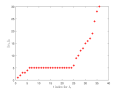
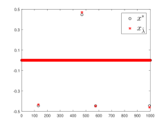
Fig. 1: Active set size on the path (left panel) on data $\{m=400,n=10^{3},s=5,\nu=0.5,\sigma=0.01,q=2.5\%\}$ and the underlying true signal $x^{*}$ and the solution $x_{\hat{\lambda}}$ selected by (18) (right panel).

5 Numerical simulation

In this section we showcase the performance of our proposed least square decoders (7) and (2). All the computations were performed on a four-core laptop with 2.90 GHz and 8 GB RAM using MATLAB 2015b. The MATLAB package 1-bitPDASC for reproducing all the numerical results can be found at http://faculty.zuel.edu.cn/tjyjxxy/jyl/list.htm.

5.1 Experiment setup

First we describe the data generation process and our parameter choice. In all numerical examples the underlying target signal $x^{*}$ with $\|x^{*}\|_{0}=s$ is given, and the observation $y$ is generated by $y=\eta\odot\textrm{sign}(\Psi x^{*}+\epsilon)$, where the rows of $\Psi$ are iid samples from $\mathcal{N}(\textbf{0},\Sigma)$ with $\Sigma_{jk}=\nu^{|j-k|},1\leq j,k\leq n$. We keep the convention $0^{0}=1.$ The elements of $\epsilon$ are generated from $\mathcal{N}(\textbf{0},\textbf{I}_{m})$, $\eta\in\mathcal{R}^{m}$ has independent coordinate $\eta_{i}$ with $\mathbb{P}[\eta_{i}=1]=1-\mathbb{P}[\eta_{i}=-1]=q$. Here, we use $\{m,n,s,\nu,\sigma,q\}$ to denote the data generated as above for short. We fix $\rho=0.95,\textsl{MaxGrid}=200,\textsl{MaxIter}=1$ in our proposed PDASC algorithm and use (18) to determine regularization parameter $\lambda$. All the simulation results are based on 100 independent replications.

5.2 Accuracy and Robustness of $x_{ls}$ when $m>n$

Now we present numerical results to illustrate the accuracy of the least square decoder $x_{ls}$ and its robustness to the noise and the sign flips. Fig. 2 shows the recovery error $\|x_{ls}-x^{*}\|$ on data set $\{m=10^{3},n=10,s=10,\nu=0.3,\sigma=0:0.05:0.5,q=2.5\%\}$. Left panel of Fig. 3 shows the recovery error $\|x_{ls}-x^{*}\|$ on data set $\{m=1000,n=10,s=10,\nu=0.3,\sigma=0.01,q=0:1\%:10\%\}$ and right panel gives recovery error $\|x_{ls}+x^{*}\|$ on data $\{m=1000,n=10,s=10,\nu=0.3,\sigma=0.01,q=90:1\%:100\%\}$. It is observed that the recovery error $\|x_{ls}-x^{*}\|$ ($\|x_{ls}+x^{*}\|$) of the least square decoder is small (around 0.1) and robust to noise level $\sigma$ and sign flips probability $q$. This confirms theoretically investigations in Theorem 2, which states the error is of order $\widetilde{\mathcal{O}}(\sqrt{\frac{n}{m}})=0.1$.

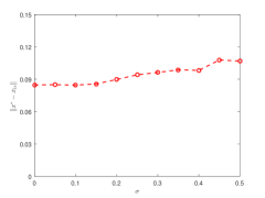
Fig. 2: Recovery error $\|x_{ls}-x^{*}\|$ v.s. $\sigma$ on $\{m=1000,n=10,s=10,\nu=0.3,\sigma=0:0.05:0.5,q=2.5\%\}$

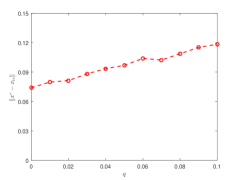
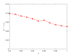
Fig. 3: Recovery error $\|x_{ls}-x^{*}\|$ v.s. $q$ on $\{m=10^{3},n=10,s=10,\nu=0.3,\sigma=0.01,q=0:1\%:10\%\}$ (left panel) and $\|-x_{ls}-x^{*}\|$ on $\{m=1000,n=10,s=10,\nu=0.3,\sigma=0.01,q=90\%:1\%:100\%\}$ (right panel).

5.3 Support recovery of $x_{\ell_{1}}$ when $m<n$

We conduct simulations to illustrate the performance of model (2) PDASC algorithm. We report how the exact support recovery probability varies with the sparsity level $s$, the noise level $\sigma$ and the probability $q$ of sign flips. Fig. 4 indicates that, as long as the sparsity level $s$ is not large, $x_{\ell_{1}}$ recovers the underlying true support with high probability even if the measurement contains noise and is corrupted by sign flips. This confirms the theoretical investigations in Theorem 3.

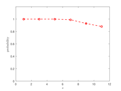
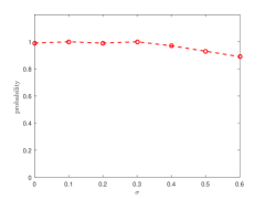
(a) $s$	(b) $\sigma$
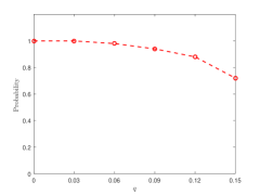
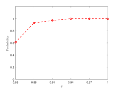
(c) $q$	(d) $q$

Fig. 4: The exact support recovery probability v.s. $s$, $\sigma$ and $q$ on data set $\{m=500,n=1000,s=1:2:12,\nu=0.1,\sigma=0.05,q=1\%\}$ (panel (a)), $\{m=500,n=1000,s=5,\nu=0.3,\sigma=0:0.1:0.6,q=5\%\}$ (panel (b)) and $\{m=500,n=1000,s=5,\nu=0.1,\sigma=0.01,q=0:3\%:15\%\}$ (panel (c)), $\{m=500,n=1000,s=5,\nu=0.1,\sigma=0.01,q=85\%:3\%:100\%\}$ (panel (d)).

5.4 Comparison with other state-of-the-art

Now we compare our proposed model (2) and PDASC algorithm with several state-of-the-art methods such as BIHT [28] (http://perso.uclouvain.be/laurent.jacques/index.php/Main/BIHTDemo), AOP [49] and PBAOP [24] (both AOP and PBAOP available at http://www.esat.kuleuven.be/stadius/ADB/huang/downloads/1bitCSLab.zip) and linear projection (LP) [47, 42]. BIHT, AOP, LP and PBAOP are all required to specify the true sparsity level $s$. Both AOP and PBAOP also need to required to specify the sign flips probability $q$. The PDASC does not require to specify the unknown parameter sparsity level $s$ or the probability of sign flips $q$. We use $\{m=500,n=1000,s=5,\nu=0.1,\sigma=0,q=0\}$, $\{m=500,n=1000,s=5,\nu=0.3,\sigma=0.3,q=5\%\}$, $\{m=500,n=1000,s=5,\nu=0.5,\sigma=0.5,q=10\%\}$, and $\{m=800,n=2000,s=10,\nu=0.1,\sigma=0.1,q=1\%\}$, $\{m=800,n=2000,s=10,\nu=0.2,\sigma=0.3,q=3\%\}$, $\{m=800,n=2000,s=10,\nu=0.3,\sigma=0.5,q=5\%\}$, and $\{m=5000,n=20000,s=50,\nu=0,\sigma=0.2,q=3\}$, $\{m=5000,n=20000,s=50,\nu=0,\sigma=0.1,q=1\}$, $\{m=5000,n=20000,s=5,\nu=0,\sigma=0.3,q=5\%\}$. The average CPU time in seconds (Time (s)), the average of the $\ell_{2}$ error $\|x_{\ell}-x^{*}\|$ ($\ell_{2}$-Err), and the probability of exactly recovering true support (PrE ($\%$)) are reported in Table 1. The PDASC is comparatively very fast and the most accurate even if the correlation $\nu$, the noise level $\sigma$ and the probability of sign flips $q$ are large.

Table 1: Comparison PDASC with state-of-the-art methods on CPU time in seconds (Time (s)), average $\ell_{2}$ error $\|x_{\ell}-x^{*}\|$ ($\ell_{2}$-Err), probability on exactly recovering of true support (PrE ($\%$)).

$\{m=500,n=1000,s=5\}$
(a) $\{\nu=0.1,\sigma=0.1,q=1\%\}$					(b) $\{\nu=0.3,\sigma=0.3,q=5\%\}$				(c) $\{\nu=0.1,\sigma=0.5,q=10\%\}$
Method	Time (s)	$\ell_{2}$-Err	PrE $(\%)$		Time (s)	$\ell_{2}$-Err	PrE $(\%)$		Time	$\ell_{2}$-Err	PrE
BIHT	1.42e-1	1.89e-1	92		1.31e-1	5.73e-1	19		1.32e-1	9.39e-1	0
AOP	2.72e-1	7.29e-2	100		3.55e-1	2.11e-1	92		3.58e-1	4.22e-1	44
LP	8.70e-3	4.19e-1	98		8.50e-3	4.22e-1	93		8.30e-3	4.81e-1	26
PBAOP	1.46e-1	9.08e-2	100		1.36e-1	2.05e-1	90		1.35e-1	4.53e-1	36
PDASC	4.11e-2	6.77e-2	100		4.38e-2	9.40e-2	99		4.56e-2	2.21e-1	71
$\{m=800,n=2000,s=10\}$
(a) $\{\nu=0.1,\sigma=0.1,q=1\%\}$					(b) $\{\nu=0.3,\sigma=0.2,q=3\%\}$				(c) $\{\nu=0.5,\sigma=0.3,q=5\%\}$
Method	Time (s)	$\ell_{2}$-Err	PrE $(\%)$		Time (s)	$\ell_{2}$-Err	PrE $(\%)$		Time	$\ell_{2}$-Err	PrE
BIHT	4.17e-1	2.10-1	84		4.25e-1	4.21e-1	25		4.35e-1	6.46e-1	0
AOP	1.09e-0	7.78-2	100		1.10e-0	1.76e-1	95		1.16e-0	2.86e-1	59
LP	1.95e-2	4.54-1	85		1.99e-2	4.49e-1	71		2.05e-2	5.03e-1	16
PBAOP	4.22e-1	1.00-1	100		4.27e-1	1.58e-1	99		4.31e-1	2.99e-1	51
PDASC	1.23e-1	8.66-2	100		1.27e-1	1.04e-1	98		1.30e-2	1.51e-1	78
$\{m=5000,n=20000,s=50,\nu=0\}$
(a) $\{\sigma=0.1,q=1\%\}$					(b) $\{\sigma=0.2,q=3\%\}$				(c) $\{\sigma=0.3,q=5\%\}$
Method	Time (s)	$\ell_{2}$-Err	PrE $(\%)$		Time (s)	$\ell_{2}$-Err	PrE $(\%)$		Time	$\ell_{2}$-Err	PrE
BIHT	2.56e+1	2.16e-1	58		2.58e+1	4.54e-1	0		2.58e+1	6.29e-1	0
AOP	6.44e+1	7.56e-2	100		6.46e+1	1.66e-1	96		6.47e+1	2.57e-1	16
LP	2.35e-1	4.47e-1	38		2.30e-1	4.46e-1	34		2.30e-1	4.47e-1	26
PBAOP	2.56e+1	9.89e-2	100		2.58e+1	1.66e-1	95		2.58e+1	2.60e-1	18
PDASC	7.09e-0	7.97e-2	100		7.17e-0	9.17e-2	99		7.23e-0	1.23e-1	86

Now we compare the PDASC with the aforementioned competitors to recover a one-dimensional signal. The true signal are sparse under wavelet basis “Db1” [36]. Thus, the matrix $\Psi$ is of size $2500\times 8000$ and consists of random Gaussian and an inverse of one level Harr wavelet transform. The target coefficient has $36$ nonzeros. We set $\sigma=0.5$, $q=4\%$. The recovered results are shown in Fig. 5 and Table 2. The reconstruction by the PHDAS is visually more appealing than others, as shown in Fig. 5. This is further confirmed by the PSNR value reported in Table 2, which is defined by $\mathrm{PSNR}=10\cdot\log\frac{V^{2}}{\rm MSE}$, where $V$ is the maximum absolute value of the true signal, and MSE is the mean squared error of the reconstruction.

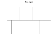
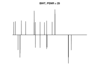
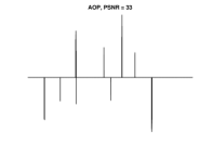
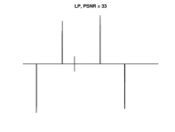
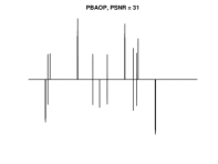
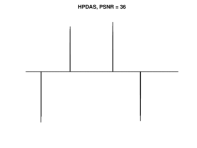
Fig. 5: Reconstruction of the one-dimension signal with $\{m=2500,n=8000,s=36,\nu=0,\sigma=0.5,q=4\%\}$.

Table 2: The CPU time in seconds and the PSNR of one dimensional signal recovery with $\{m=2500,n=8000,s=36,\nu=0,\sigma=0.5,q=4\%\}$.

method	CPU time (s)	PSNR
BIHT	4.97	29
AOP	4.98	33
LP	0.11	33
PBAOP	4.93	31
PDASC	3.26	36

6 Conclusions

In this paper we consider decoding from 1-bit measurements with noise and sign flips. For $m>n$, we show that, up to a constant $c$, with high probability the least squares solution $x_{\textrm{ls}}$ approximates $x^{*}$ with precision $\delta$ as long as $m\geq\widetilde{\mathcal{O}}(\frac{n}{\delta^{2}})$. For $m<n$, we assume that the underlying target $x^{*}$ is $s$-sparse, and prove that up to a constant $c$, with high probability, the $\ell_{1}$-regularized least squares solution $x_{\ell_{1}}$ lies in the ball with center $x^{*}$ and radius $\delta$, provided that $m\geq\mathcal{O}(\frac{s\log n}{\delta^{2}})$. We introduce the one-step convergent PDAS method to minimize the nonsmooth objection function. We propose a novel tuning parameter selection rule which is seamlessly integrated with the continuation strategy without any extra computational overhead. Numerical experiments are presented to illustrate salient features of the model and the efficiency and accuracy of the algorithm.

There are several avenues for further study. First, many practitioners observed that nonconvex sparse regularization often brings in additional benefit in the standard CS setting. Whether the theoretical and computational results derived in this paper can still be justified when nonconvex regularizers are used deserves further consideration. The 1-bit CS is a kind of nonlinear sampling approach. Analysis of some other nonlinear sampling methods are also of immense interest.

Appendix A Proof of Lemma 3

Proof.

Let $u=\tilde{\psi}^{t}x^{*}$. Then $u\sim\mathcal{N}(0,1)$ due to $\tilde{\psi}\sim\mathcal{N}(\textbf{0},\Sigma)$ and the assumption that $\|x^{*}\|_{\Sigma}=1.$

$$\mathbb{E}[\tilde{\psi}\tilde{y}] =\mathbb{E}[\tilde{\psi}\tilde{\eta}\textrm{sign}(\tilde{\psi}^{t}x^{*}+\tilde{\epsilon})]=\mathbb{E}[\tilde{\eta}]\mathbb{E}[\tilde{\psi}\textrm{sign}(\tilde{\psi}^{t}x^{*}+\tilde{\epsilon})]$$

$$=[q-(1-q)]\mathbb{E}[\tilde{\psi}\textrm{sign}(\tilde{\psi}^{t}x^{*}+\tilde{\epsilon})]$$

$$=(2q-1)\mathbb{E}[\mathbb{E}[\tilde{\psi}\textrm{sign}(\tilde{\psi}^{t}x^{*}+\tilde{\epsilon})|\tilde{\psi}^{t}x^{*}]]$$

$$=(2q-1)\mathbb{E}[\mathbb{E}[\tilde{\psi}|\tilde{\psi}^{t}x^{*}]\textrm{sign}(\tilde{\psi}^{t}x^{*}+\tilde{\epsilon})]$$

$$=(2q-1)\mathbb{E}[\mathbb{E}[\tilde{\psi}|\tilde{\psi}^{t}x^{*}]\mathbb{E}[\textrm{sign}(\tilde{\psi}^{t}x^{*}+\tilde{\epsilon})|\tilde{\psi}^{t}x^{*}]]$$

$$=(2q-1)\mathbb{E}[\Sigma x^{*}\tilde{\psi}^{t}x^{*}\mathbb{E}[\textrm{sign}(\tilde{\psi}^{t}x^{*}+\tilde{\epsilon})|\tilde{\psi}^{t}x^{*}]]$$

$$=(2q-1)\mathbb{E}[\textrm{sign}(\tilde{\psi}^{t}x^{*}+\tilde{\epsilon})\tilde{\psi}^{t}x^{*}]\Sigma x^{*}$$

$$=c\Sigma x^{*},$$

where $c=(2q-1)\mathbb{E}[\textrm{sign}(\tilde{\psi}^{t}x^{*}+\tilde{\epsilon})\tilde{\psi}x^{*}]$. The second line follows from independence assumption and the third from law of total expectation, and the fourth and fifth lines are due to the independence between $\tilde{\epsilon}$ and $u$, and the sixth line uses the projection interpretation of conditional expectation i.e., $\mathbb{E}[\tilde{\psi}|\tilde{\psi}^{t}x^{*}]=\frac{\mathbb{E}[\tilde{\psi}\tilde{\psi}^{t}x^{*}]-\mathbb{E}[\tilde{\psi}^{t}x^{*}]\mathbb{E}[\tilde{\psi}]}{\mathbb{E}[(\tilde{\psi}^{t}x^{*}-\mathbb{E}[\tilde{\psi}^{t}x^{*}])^{2}]}(\tilde{\psi}^{t}x^{*}-\mathbb{E}[\tilde{\psi}^{t}x^{*}])+\mathbb{E}[\tilde{\psi}]=\Sigma x^{*}\tilde{\psi}^{t}x^{*}$, where we use $\mathbb{E}[\tilde{\psi}]=\textbf{0}$ and $u\sim\mathcal{N}(0,1)$. Let $f(t)=\frac{1}{\sqrt{2\pi}\sigma}\exp{\frac{-t^{2}}{2\sigma^{2}}}$ be the density function of $\tilde{\epsilon}\sim\mathcal{N}(0,\sigma^{2})$. Integrating by parts shows that

$$c=(2q-1)\mathbb{E}[\textrm{sign}(u+\tilde{\epsilon})u] =(2q-1)\mathbb{E}[(1-2\mathbb{P}[\tilde{\epsilon}\leq-u])u]$$

$$=(2q-1)\mathbb{E}[\frac{\partial(1-2\mathbb{P}[\tilde{\epsilon}\leq-u)}{\partial u}]$$

$$=(2q-1)\mathbb{E}[f(-u)]=(2q-1)\sqrt{\frac{2}{\pi(\sigma^{2}+1)}}.$$

The proof is completed by inverting $c\Sigma$. ∎

Appendix B Preliminaries

We recall some simple properties of subgaussian and subexponential random variables.

Lemma 5.

( Lemma 2.7.7 of [48] and Remark 5.18 of [46].) Let $\xi_{1}$ and $\xi_{2}$ be subgaussian random variables. Then both $\xi_{1}\xi_{2}$ and $\xi_{1}\xi_{2}-\mathbb{E}[\xi_{1}\xi_{2}]$ are subexponential random variables.

Lemma B.2 states the nonasymptotic bound on the spectrums of $\Psi$ and the operator norm of $\Psi^{t}\Psi/m-\Sigma$ when $m\geq\mathcal{O}(n).$

Lemma 6.

Let $\Psi\in\mathcal{R}^{m\times n}$ whose rows $\psi_{i}^{t}$ are independent subgaussian vectors in $\mathcal{R}^{n}$ with mean 0 and covariance matrix $\Sigma$. Let $m>n$. Then for every $t>0$ with probability at least $1-2\exp{(-C_{1}t^{2})}$, one has

$$(1-\tau)\sqrt{\gamma_{min}(\Sigma)}\leq\sqrt{\gamma_{\textrm{min}}(\frac{\Psi^{t}\Psi}{m})}\leq\sqrt{\gamma_{\textrm{max}}(\frac{\Psi^{t}\Psi}{m})}\leq(1+\tau)\sqrt{\gamma_{max}(\Sigma)},$$ (19)

and

$$\|\Psi^{t}\Psi/m-\Sigma\|\leq\max\{\tau,\tau^{2}\}\gamma_{\textrm{max}}(\Sigma),$$ (20)

where $\tau=C_{2}\sqrt{\frac{n}{m}}+\frac{t}{\sqrt{m}},$ and $C_{1},C_{2}$ are generic positive constants depending on the maximum subgaussian norm of rows of $\Psi$.

Proof.

Let $\Phi=\Psi\Sigma^{-\frac{1}{2}}$. Then the rows of $\Phi$ are independent sub-gaussian isotropic vectors. (19) follows from Theorem 5.39 and Lemma 5.36 of [46] and (20) is a direct consequence of Remark 5.40 of [46].

∎

We state the Bernstein-type inequality for the sum of independent and mean $0$ sub-exponential random random variables.

Lemma 7.

(Corollary 5.17 of [46]) Let $\xi_{1},...,\xi_{m}$ be independent centered sub-exponential random variables. Then for every $t>0$ one has

$$\mathbb{P}[|\sum_{i=1}^{m}\xi_{i}|/m\geq t]\leq 2\exp(-\min\{C_{1}t^{2},C_{2}t\}m)$$

where $C_{1}$ and $C_{2}$ are are generic positive constants depending on the maximum subexponential norm of of $\xi_{i}$.

Lemma 8.

Let $\Psi\in\mathcal{R}^{m\times n}$ whose rows $\psi_{i}$ are independent subgaussian vectors in $\mathcal{R}^{n\times 1}$ with mean 0 and covariance matrix $\Sigma$. Then, with probability at least $1-2\exp{(-C_{1}C_{2}^{2}n)}$,

$$\|\Psi^{t}\Psi/m-\mathbb{E}[\Psi^{t}\Psi/m]\|\leq 2C_{2}\gamma_{\textrm{max}}(\Sigma)\sqrt{\frac{n}{m}},$$ (21)

as long as $m\geq 4C^{2}_{2}n$. Furthermore, if $m>\frac{4C_{1}}{C_{2}^{2}}\log n$, then

$$\|\sum_{i=1}^{m}(\mathbb{E}[\psi_{i}y_{i}]-\psi_{i}y_{i})/m\|_{\infty}\leq 2\sqrt{\frac{\log n}{C_{1}m}},$$ (22)

holds with probability at least $1-\frac{2}{n^{3}},$ and

$$\|\Psi^{t}\Psi/m-\Sigma\|_{\infty}\leq 2\sqrt{\frac{\log n}{C_{1}m}},$$ (23)

holds with probability at least $1-\frac{1}{n^{2}}.$

Proof.

By (5), $\mathbb{E}[\Psi^{t}\Psi/m]=\Sigma$, hence (21) follows from (20) with $t=C_{2}\sqrt{n}$ and the assumption $m\geq 4C^{2}_{2}n$. Define $G_{i,j}:=y_{i}(\psi_{i})_{j}\in\mathcal{R}^{1},i=1,...,m,j=1,..,n,$ which is subexponential by Lemma 5. Therefore,

$$\mathbb{P}[\|\sum_{i=1}^{m}(\mathbb{E}[\psi_{i}y_{i}]-\psi_{i}y_{i})/m\|_{\infty}\geq t] =\mathbb{P}[\bigcup_{j=1}^{n}\{|\sum_{i=1}^{m}G_{i,j}/m|\geq t\}]$$

$$\leq\sum_{j=1}^{n}\mathbb{P}[|\sum_{i=1}^{m}G^{(i)}_{k,j}|/m\geq t]$$

$$\leq n\exp(-\min\{C_{1}t^{2},C_{2}t\}m)$$

$$\leq 2n\exp(-C_{1}t^{2}m),$$

where the first inequality is due to the union bound, the second follows from Lemma 7 and the last is because of restrictions $t\leq\frac{C_{2}}{C_{1}}$ and $m<n.$ Then (22) follows from our assumption that $m>\frac{4C_{1}}{C_{2}^{2}}\log n$ by setting $t=2\sqrt{\frac{\log n}{C_{1}m}}$ and. Let $G_{j,k}^{i}:=(\psi_{i})_{j}(\psi_{i})_{k}-\Sigma_{j,k}\in\mathcal{R}^{1},i=1,...,n,j=1,...,n,\ell=1,..,n,$ which is mean $0$ subexponential by Lemma 5. Therefore,

$$\mathbb{P}[\|\Psi^{t}\Psi/m-\Sigma\|_{\infty}\geq t] =\mathbb{P}[\max_{j,k}|\sum_{i=1}^{m}G_{j,k}^{i}/m|\geq t]$$

$$=\mathbb{P}[\bigcup_{j=1,k=1}^{n,n}\{|\sum_{i=1}^{m}G_{j,k}^{i}/m|\geq t\}]$$

$$\leq\sum_{j=1,k=1}^{n,n}\mathbb{P}[|\sum_{i=1}^{m}G_{j,k}^{i}/m|\geq t]$$

$$\leq n^{2}\exp(-\min\{C_{1}t^{2},C_{2}t\}m)$$

$$\leq n^{2}\exp(-C_{1}t^{2}m),$$

where the first inequality is due to the union bound, and the second follows from Lemma 7 and the last inequality is because of restricting $t\leq\frac{C_{2}}{C_{1}}$. Then by the assumption that $m>\frac{4C_{1}}{C_{2}^{2}}\log n$, Lemma 23 follows by setting $t=2\sqrt{\frac{\log n}{C_{1}m}}$. ∎

Appendix C Proof of Theorem 2

Proof.

First we show that the sample covariance matrix $\Psi^{t}\Psi/m$ is invertible with probability at least $1-2\exp{(-C_{1}C_{2}^{2}n)}$ as long as $m>4C_{2}n.$ This follows from (19) in Lemma 6 by setting $t=C_{2}\sqrt{n}$. Recall

$$\widetilde{x}^{*}=cx^{*}.$$ (24)

Let

$$\Delta=y-\Psi\widetilde{x}^{*},$$ (25)

be the error in measuring nonlinearity, sign flips and noise in the 1-bit CS measurement. Then,

$$\|\Psi^{t}\Delta/m\|_{2} =\|\Psi^{t}(\Psi\widetilde{x}^{*}-y)/m\|_{2}=\|\frac{\Psi^{t}\Psi}{m}\widetilde{x}^{*}-\Psi^{t}y/m\|_{2}=\|(\frac{\Psi^{t}\Psi}{m}\widetilde{x}^{*}-\Sigma\widetilde{x}^{*})+(\Sigma\widetilde{x}^{*}-\Psi^{t}y/m)\|_{2}$$

$$=\|(\frac{\Psi^{t}\Psi}{m}\widetilde{x}^{*}-\mathbb{E}[\frac{\Psi^{t}\Psi}{m}\widetilde{x}^{*}])+(\mathbb{E}[\Psi^{t}y/m]-\Psi^{t}y/m)\|_{2}$$

$$\leq|c|\|{x^{*}}\|_{2}\|\frac{\Psi^{t}\Psi}{m}-\mathbb{E}[\frac{\Psi^{t}\Psi}{m}]\|+\|\sum_{i=1}^{m}(\mathbb{E}[\psi_{i}y_{i}]-\psi_{i}y_{i})/m\|_{2}$$

$$\leq|c|\frac{1}{\sqrt{\gamma_{\textrm{min}}(\Sigma)}}\|\frac{\Psi^{t}\Psi}{m}-\mathbb{E}[\frac{\Psi^{t}\Psi}{m}]\|+\sqrt{n}\|\sum_{i=1}^{m}(\mathbb{E}[\psi_{i}y_{i}]-\psi_{i}y_{i})/m\|_{\infty},$$ (26)

where the fourth equality is due to (3), (5) and (6), the first inequality follows from the triangle inequality and the definition of $\widetilde{x}^{*}$, and the last inequality uses the assumption $1=\|x^{*}\|^{2}_{\Sigma}\geq\gamma_{\textrm{min}}(\Sigma)\|x^{*}\|_{2}^{2}$ and the fact that $\|\cdot\|_{2}\leq\sqrt{n}\|\cdot\|_{\infty}$. Combining with (21) and $\eqref{linfnoise2}$, we deduce that, with probability at least $1-2\exp{(-C_{1}C_{2}^{2}n)}-\frac{2}{n^{3}}$,

$$\|\Psi^{t}\Delta/m\|_{2}\leq\sqrt{\frac{n}{m}}2(|c|C_{2}\sqrt{\kappa(\Sigma)\gamma_{\textrm{max}}(\Sigma)}+\sqrt{\frac{\log n}{C_{1}}}).$$ (27)

Now we prove that $\|x_{\textrm{ls}}/c-cx^{*}\|_{2}=\widetilde{\mathcal{O}}(\sqrt{\frac{n}{m}}/c)$ with high probability.

$$|c|\|x_{\textrm{ls}}/c-x^{*}\|_{2} =\|x_{\textrm{ls}}-\widetilde{x}^{*}\|_{2}=\|(\Psi^{t}\Psi)^{-1}\Psi^{t}y-\widetilde{x}^{*}\|_{2}$$

$$\leq\|(\Psi^{t}\Psi/m)^{-1}\Psi^{t}(\Psi\widetilde{x}^{*}+y-\Psi\widetilde{x}^{*})/m-\widetilde{x}^{*}\|_{2}$$

$$=\|(\Psi^{t}\Psi/m)^{-1}\|\|\Psi^{t}\Delta/m\|_{2}$$

$$\leq\sqrt{\frac{n}{m}}2(|c|C_{2}\sqrt{\kappa(\Sigma)\gamma_{\textrm{max}}(\Sigma)}+\sqrt{\frac{\log n}{C_{1}}})/(1-2C_{2}\sqrt{\frac{n}{m}})^{2}$$

$$\leq\sqrt{\frac{n}{m}}4(|c|C_{2}\sqrt{\kappa(\Sigma)\gamma_{\textrm{max}}(\Sigma)}+\sqrt{\frac{\log n}{C_{1}}}),$$

where the second inequality follows with probability at least $1-4\exp{(-C_{1}C_{2}^{2}n)}-\frac{2}{n^{3}}$ from (26) and (19) by setting $t=C_{2}\sqrt{n}$, and the last line is due to the assumption $m\geq 16C_{2}^{2}n.$ Hence, the proof of Theorem 2 is completed by dividing $|c|$ on both side and some algebra. ∎

Appendix D Proof of Theorem 3

Proof.

Our proof is based on Lemmas 9 - 11 below. Denote $R=x_{\ell_{1}}-\widetilde{x}^{*}$, $\mathcal{A}^{*}=supp(x^{*})$ and $\mathcal{I}^{*}=\overline{\mathcal{A}^{*}}$. The first lemma shows that $R$ is sparse in the sense that its energy is mainly cumulated on $\mathcal{A}^{*}$ if $\lambda$ is chosen properly.

Lemma 9.

Let

$$\mathcal{C}_{\mathcal{A^{*}}}=\{z\in\mathcal{R}^{n}:\|z_{\mathcal{I^{*}}}\|_{1}\leq 3\|z_{\mathcal{A^{*}}}\|_{1}\},$$ (28)

and define $\mathcal{E}=\{\|\Psi^{t}\Delta/m\|_{\infty}\leq\lambda/2\}$. Conditioning on the event $\mathcal{E}$, we have $R\in\mathcal{C}_{\mathcal{A^{*}}}$.

Proof.

The optimality of $x_{\ell_{1}}$ implies that $\frac{1}{2m}\|y-\Psi x_{\ell_{1}}\|_{2}^{2}+\lambda\|x_{\ell_{1}}\|_{1}\leq\frac{1}{2m}\|y-\Psi\widetilde{x}^{*}\|_{2}^{2}+\lambda\|\widetilde{x}^{*}\|_{1}.$ Recall that $y=\Psi\widetilde{x}^{*}+\Delta$. Some algebra on the above display shows

$$\frac{1}{2m}\|\Psi R\|_{2}^{2}+\lambda\|R_{\mathcal{I}^{*}}\|_{1}\leq\langle R,\Psi^{t}\Delta/m\rangle+\lambda\|R_{\mathcal{A}^{*}}\|_{1}$$

$$\leq\|R\|_{1}\|\Psi^{t}\Delta/m\|_{\infty}+\lambda\|R_{\mathcal{A}^{*}}\|_{1}\leq\|R\|_{1}\lambda/2+\lambda\|R_{\mathcal{A}^{*}}\|_{1},$$

where, we use Cauchy Schwartz inequality and the definition of $\mathcal{E}$. The above inequality shows

$$\frac{1}{m}\|\Psi R\|_{2}^{2}+\lambda\|R_{\mathcal{I}^{*}}\|_{1}\leq 3\lambda\|R_{\mathcal{A}^{*}}\|_{1},$$ (29)

i.e., $R\in\mathcal{C}_{\mathcal{A^{*}}}$. This finishes the proof of Lemma 9. ∎

The next Lemma gives a lower bound on $\mathbb{P}[\mathcal{E}]$ with a proper regularization parameter $\lambda$.

Lemma 10.

Let $C_{3}\geq\|x^{*}\|_{1}$. If $m>\frac{4C_{1}}{C_{2}^{2}}\log n$, taking $\lambda=\frac{4(1+|c|C_{3})}{\sqrt{C_{1}}}\sqrt{\frac{\log n}{m}}$, then with probability at least $1-2/n^{3}-2/n^{2}$, one has

$$\|\Psi^{t}\Delta/m\|_{\infty}\leq\lambda/2.$$ (30)

Proof.

$$\|\Psi^{t}\Delta/m\|_{\infty} =\|\Psi^{t}(\Psi\widetilde{x}^{*}-y)/m\|_{\infty}=\|(\frac{\Psi^{t}\Psi}{m}\widetilde{x}^{*}-\Sigma\widetilde{x}^{*})+(\Sigma\widetilde{x}^{*}-\Psi^{t}y/m)\|_{\infty}$$

$$\leq\|(\frac{\Psi^{t}\Psi}{m}\widetilde{x}^{*}-\Sigma\widetilde{x}^{*})\|_{\infty}+\|(\mathbb{E}[\Psi^{t}y/m]-\Psi^{t}y/m)\|_{\infty}$$

$$\leq|c|\|(\frac{\Psi^{t}\Psi}{m}-\Sigma)\|_{\infty}\|x^{*}\|_{1}+\|\sum_{i=1}^{m}(\mathbb{E}[\psi_{i}y_{i}]-\psi_{i}y_{i})/m\|_{\infty}$$

$$\leq|c|C_{3}2\sqrt{\frac{\log n}{C_{1}m}}+2\sqrt{\frac{\log n}{C_{1}m}}$$

$$=\frac{2(1+|c|C_{3})}{\sqrt{C_{1}}}\sqrt{\frac{\log n}{m}},$$

where the first inequality is due to the triangle inequality, (3), (5) and (6), the second inequality follows from the definition of $\widetilde{x}^{*}$ and Cauchy-Schwartz inequality, and the third one uses (22) and (23). The proof of Lemma 10 is completed by setting $\lambda=\frac{4(1+|c|C_{3})}{\sqrt{C_{1}}}\sqrt{\frac{\log n}{m}}$. ∎

The last Lemma shows $\Psi$ is strongly convex along the direction contained in the cone $\mathcal{C}_{\mathcal{A^{*}}}$ defined in (28).

Lemma 11.

If $s\leq\exp^{(1-\frac{C_{1}}{2})}n$ and $m\geq\frac{64(4\kappa(\Sigma)+1)^{2}}{C_{1}}s\log\frac{en}{s},$ then with probability at least $1-1/n^{2}$, we have

$$\|\Psi z\|^{2}_{2}/m\geq\frac{\gamma_{min}(\Sigma)}{68(4\kappa(\Sigma)+1)^{2}}\|z\|_{2}^{2},\quad\forall z\in\mathcal{C}_{\mathcal{A^{*}}}.$$

Proof.

$\forall z\in\mathcal{C}_{\mathcal{A^{*}}}=\{v\in\mathcal{R}^{n}:\|v_{\mathcal{I^{*}}}\|_{1}\leq 3\|v_{\mathcal{A^{*}}}\|_{1}\}$, we sort its entries such that

$$|z_{k_{1}}|\geq|z_{k_{2}}|\geq...\geq|z_{k_{n}}|.$$

Let $\mathcal{A}=\{k_{1},...,k_{s}\}$, and $\mathcal{I}=\bigcup_{t\geq 1}\mathcal{I}_{t}=\{k_{st+1},...,k_{(t+1)s}\},$ where $s=\|x^{*}\|_{0}.$ Then

$$\|z_{\mathcal{I}}\|_{1}\leq 3\|z_{\mathcal{A}}\|_{1}.$$ (31)

By the elementary inequality $\|v\|_{2}\leq\frac{\|v\|_{1}}{\sqrt{s}}+\frac{\sqrt{s}\|v\|_{\infty}}{4},\quad\forall v\in\mathcal{R}^{s},$ we have

$$\sum_{t\geq 1}\|z_{\mathcal{I}_{t}}\|_{2} \leq\sum_{t\geq 1}\frac{\|z_{\mathcal{I}_{t}}\|_{1}}{\sqrt{s}}+\frac{\sqrt{s}\|z_{\mathcal{I}_{t}}\|_{\infty}}{4}$$

$$=\frac{\|z_{\mathcal{I}}\|_{1}}{\sqrt{s}}+\sum_{t\geq 1}\frac{\sqrt{s}\|z_{k_{st+1}}\|_{\infty}}{4}$$

$$\leq\frac{\|z_{\mathcal{I}}\|_{1}}{\sqrt{s}}+\frac{\|z_{\mathcal{A}}\|_{1}+\|z_{\mathcal{I}}\|_{1}}{4\sqrt{s}}$$

$$\leq\frac{3\|z_{\mathcal{A}}\|_{1}}{\sqrt{s}}+\frac{\|z_{\mathcal{A}}\|_{1}+3\|z_{\mathcal{A}}\|_{1}}{4\sqrt{s}}\quad(using\quad\eqref{nnc})$$

$$=\frac{4\|z_{\mathcal{A}}\|_{1}}{\sqrt{s}}$$

$$\leq 4\|z_{\mathcal{A}}\|_{2},$$ (32)

which implies,

$$\|z\|_{2}^{2}=\|z_{\mathcal{A}}\|_{2}^{2}+\sum_{t\geq 1}\|z_{\mathcal{I}_{t}}\|_{2}^{2}\leq\|z_{\mathcal{A}}\|_{2}^{2}+(\sum_{t\geq 1}\|z_{\mathcal{I}_{t}}\|_{2})^{2}=17\|z_{\mathcal{A}}\|_{2}^{2}.$$ (33)

Define

$$C_{2s}(\Psi)=\inf_{A\subset[n],|A|\leq 2s}\frac{\gamma_{min}(\Psi_{A}^{t}\Psi_{A})}{m},$$

and

$$O_{s}(\Psi)=\sup_{A,B\subset[n],A\cap B=\emptyset,|A|\leq s,|B|\leq s}\|\Psi_{A}^{t}\Psi_{B}/m\|.$$

We obtain that,

$$\langle\Psi_{\mathcal{A}}z_{\mathcal{A}},\Psi_{\mathcal{I}}z_{\mathcal{I}}\rangle/m =\langle\Psi_{\mathcal{A}}z_{\mathcal{A}},\sum_{t\geq 1}\Psi_{\mathcal{I}_{t}}z_{\mathcal{I}_{t}}\rangle/m$$

$$\leq\|z_{\mathcal{A}}\|_{2}\sum_{t\geq 1}\|\Psi^{t}_{\mathcal{A}}\Psi_{\mathcal{I}_{t}}\|_{2}\|z_{\mathcal{I}_{t}}\|_{2}$$

$$\leq O_{s}(\Psi)\|z_{\mathcal{A}}\|_{2}\sum_{t\geq 1}\|z_{\mathcal{I}_{t}}\|_{2}$$

$$\leq 4O_{s}(\Psi)\|z_{\mathcal{A}}\|^{2},$$ (34)

where the first inequality uses Cauchy-Schwartz inequality, the second inequality follows from the definition of $O_{s}(\Psi),$ and the third is due to (32). Then, $\forall z\in\mathcal{C}_{\mathcal{A^{*}}},z\neq 0,$ we have

$$\|\Psi z\|^{2}_{2}/(m\|z\|^{2})\geq\|\Psi z\|^{2}_{2}/(17m\|z_{\mathcal{A}}\|^{2})$$

$$=(\|\Psi_{\mathcal{A}}z_{\mathcal{A}}\|^{2}+\|\Psi_{\mathcal{I}}z_{\mathcal{I}}\|^{2}+2\langle\Psi_{\mathcal{A}}z_{\mathcal{A}},\Psi_{\mathcal{I}}z_{\mathcal{I}}\rangle)/(17m\|z_{\mathcal{A}}\|^{2})$$

$$\geq(\|\Psi_{\mathcal{A}}z_{\mathcal{A}}\|^{2}-8O_{s}(\Psi)\|z_{\mathcal{A}}\|^{2})/(17m\|z_{\mathcal{A}}\|^{2})$$

$$\geq(C_{2s}(\Psi)-8O_{s}(\Psi))/17,$$ (35)

where the first inequality uses (33), the second inequality follows from (34), and the last holds due to the definition of $C_{2s}(\Psi).$ It follows from (35) that, to complete the proof of this lemma it suffices to derive a lower bound on $C_{2s}(\Psi)$ and an upper bound on $O_{s}(\Psi)$ with high probability, respectively. Given $A\subset[n],|A|\leq 2s$, we define the event $E_{A}=\{\sqrt{\frac{\gamma_{min}(\Psi_{A}^{t}\Psi_{A})}{m}}>\sqrt{\gamma_{min}(\Sigma)}(1-C_{2}\sqrt{\frac{2s}{m}}-\frac{t}{\sqrt{m}})\}$. Then,

$$\mathbb{P}[C_{2s}(\Psi)>\gamma_{min}(\Sigma)(1-C_{2} \sqrt{\frac{2s}{m}}-\frac{t}{\sqrt{m}})^{2}]=\mathbb{P}[\bigcap_{A\in[n],|A|\leq 2s}E_{A}]=\mathbb{P}[\bigcap_{A\in[n],|A|=\ell,1\leq\ell\leq 2s}E_{A}]$$

$$=1-\mathbb{P}[\bigcup_{A\in[n],|A|=\ell,1\leq\ell\leq 2s}\overline{E_{A}}]$$

$$\geq 1-\sum_{\ell=1}^{2s}\sum_{A\subset[n],|A|=\ell}(1-\mathbb{P}[E_{A}])$$

$$\geq 1-\sum_{\ell=1}^{2s}\sum_{A\subset[n],|A|\leq\ell}2\exp(-C_{1}t^{2})$$

$$=1-\sum_{\ell=1}^{2s}\binom{n}{\ell}2\exp(-C_{1}t^{2})$$

$$\geq 1-2(\frac{en}{2s})^{2s}\exp(-C_{1}t^{2}),$$

where the first inequality follows from the union bound, the second inequality follows from (19) by replacing $\Psi$ with $\Psi_{A}$, and the third inequality holds since $\sum_{\ell=1}^{2s}\binom{n}{\ell}\leq(\frac{n}{2s})^{2s}\sum_{\ell=0}^{2s}\binom{n}{\ell}(\frac{2s}{n})^{\ell}\leq(\frac{n}{2s})^{2s}(1+\frac{2s}{n})^{n}\leq(\frac{en}{2s})^{2s}$. Then, we derive with probability at least $1-2(\frac{en}{2s})^{2s}\exp(-C_{1}t^{2}),$

$$C_{2s}(\Psi)>\gamma_{min}(\Sigma)(1-C_{2}\sqrt{\frac{2s}{m}}-\frac{t}{\sqrt{m}})^{2}.$$ (36)

Given $A\subset[n],B\subset[n],|A|\leq s,|B|\leq s,A\cap B=\emptyset$, we define the event $E_{A,B}=\{\|\Psi_{A}^{t}\Psi_{B}/m\|>\gamma_{max}(\Sigma)(C_{2}\sqrt{\frac{2s}{m}}+\frac{t}{\sqrt{m}})\}$. Denote $C=A\cup B,$ $\Phi_{C}=\Psi_{C}\Sigma_{CC}^{-\frac{1}{2}}$, $G_{C}=\Phi_{C}^{t}\Phi_{C}/m-\textbf{I}_{2s}$. Then each row of $\Phi_{C}$ is multivariate normal random vector that is sampled from $\mathcal{N}(\textbf{0},\textbf{I}_{2s})$. It follows from (20) with $\Psi$ and $\Sigma$ replaced by $\Phi_{C}$ and $\textbf{I}_{2s}$, respectively, that

$$\mathbb{P}[\|G_{C}\|\geq C_{2}\sqrt{\frac{2s}{m}}+\frac{t}{\sqrt{m}}]\leq 2\exp{(-C_{1}t^{2})}.$$

Observing $\Sigma_{CC}^{-\frac{1}{2}}\Psi_{A}^{t}\Psi_{B}\Sigma_{CC}^{-\frac{1}{2}}/m$ is a sub-matrix of $G_{C}$, we deduce,

$$\mathbb{P}[E_{A,B}]\leq 2\exp{(-C_{1}t^{2})}.$$

Then, similarly to the proof of (36), we have

$$\mathbb{P}[O_{s}(\Psi)>\gamma_{max}(\Sigma)(C_{2}\sqrt{\frac{2s}{m}}+\frac{t}{\sqrt{m}})] =\mathbb{P}[\bigcup_{A,B\subset[n],A\cap B=\emptyset,|A|\leq s,|B|\leq s}E_{A,B}]$$

$$=\mathbb{P}[\bigcup_{A\subset[n],|A|=\ell,B\subset[n],|B|=\tilde{\ell},A\cap B=\emptyset,1\leq\ell\leq s,1\leq\tilde{\ell}\leq s}E_{A,B}]$$

$$\leq\sum_{\ell=1,\tilde{\ell}=1}^{s}\sum_{A\in[n],|A|\leq\ell,B\in[n],|B|\leq\tilde{\ell},A\cap B=\emptyset}2\exp(-C_{1}t^{2})$$

$$\leq(\sum_{\ell=1}^{s}\binom{n}{\ell})^{2}2\exp(-C_{1}t^{2})$$

$$\leq 2(\frac{en}{s})^{2s}\exp(-C_{1}t^{2}),$$

which implies with probability at least $1-2(\frac{en}{s})^{2s}\exp(-C_{1}t^{2})$,

$$O_{s}(\Psi)\leq\gamma_{max}(\Sigma)(C_{2}\sqrt{\frac{2s}{m}}+\frac{t}{\sqrt{m}}).$$ (37)

Combining (36) and (37) and setting $t=\sqrt{\frac{4s}{C_{1}}\log\frac{en}{s}}$, we obtain that with probability at least $1-4/(\frac{en}{s})^{2s}\geq 1-4/n^{2}$

$$C_{2s}(\Psi)-8O_{s}(\Psi)\geq\gamma_{min}(\Sigma)f\big{(}\sqrt{\frac{2s}{m}}+\sqrt{\frac{4s}{mC_{1}}\log\frac{en}{s}}\big{)},$$

where the unitary function $f(z)=z^{2}-(8\kappa(\Sigma)+2)z+1$. It follows from the assumption $s\leq\exp^{(1-\frac{C_{1}}{2})}n$ that $\sqrt{\frac{2s}{m}}\leq\sqrt{\frac{4s}{mC_{1}}\log\frac{en}{s}}$. Then some basic algebra shows that $f\big{(}\sqrt{\frac{2s}{m}}+\sqrt{\frac{4s}{mC_{1}}\log\frac{en}{s}}\big{)}\geq f(\frac{1}{8\kappa(\Sigma)+2})=\frac{1}{4(4\kappa(\Sigma)+1)^{2}}$ as long as $m\geq\frac{64(4\kappa(\Sigma)+1)^{2}}{C_{1}}s\log\frac{en}{s}$. The proof of Lemma 11 is completed. ∎

Now we are in the place of combining the above pieces together to finish the proof of Theorem 3. Recall $R=x_{\ell_{1}}-\widetilde{x}^{*}$. It follows from Lemma 9 that $R\in\mathcal{C}_{\mathcal{A}^{*}}$ and (29) holds by conditioning on $\mathcal{E}$, i.e.,

$$\frac{1}{m}\|\Psi R\|_{2}^{2}+\lambda\|R_{\mathcal{I}^{*}}\|_{1}\leq 3\lambda\|R_{\mathcal{A}^{*}}\|_{1},$$

which together with Lemma 11 implies that, with probability at least $1-4/n^{2}$,

$$\frac{\gamma_{min}(\Sigma)}{68(4\kappa(\Sigma)+1)^{2}}\|R\|_{2}^{2}\leq 3\lambda\|R_{\mathcal{A}^{*}}\|_{1}\leq 3\lambda\sqrt{s}\|R_{\mathcal{A}^{*}}\|_{2},$$

i.e.,

$$|c|\|x_{\ell_{1}}/c-{x}^{*}\|_{2}=\|x_{\ell_{1}}-\widetilde{x}^{*}\|_{2}\leq\frac{204(4\kappa(\Sigma)+1)^{2}}{\gamma_{min}(\Sigma)}\lambda\sqrt{s}.$$

The proof of Theorem 3 is completed by dividing $|c|$ on both side and using Lemma 10, which guaranties that $\eqref{basiceq}$ holds with $\lambda=\frac{4(1+|c|C_{3})}{\sqrt{C_{1}}}\sqrt{\frac{\log n}{m}}$ with probability greater than $1-2/n^{3}-2/n^{2}$. ∎

Appendix E Proof of the equivalency between the PDAS and (15) - (16)

Proof.

Partition $Z^{k}$, $D^{k}$ and $F(Z^{k})$ according to $\mathcal{A}_{k}$ and $\mathcal{I}_{k}$ such that

$$Z^{k}=\left(\begin{array}[]{c}x_{\mathcal{A}_{k}}\\ x_{\mathcal{I}_{k}}\\ d_{\mathcal{A}_{k}}\\ d_{\mathcal{I}_{k}}\\ \end{array}\right),$$

$$D^{k}=\left(\begin{array}[]{c}D^{x}_{\mathcal{A}_{k}}\\ D^{x}_{\mathcal{I}_{k}}\\ D^{d}_{\mathcal{A}_{k}}\\ D^{d}_{\mathcal{I}_{k}}\\ \end{array}\right),$$ (38)

$$F(Z^{k})=\left[\begin{array}[]{c}-d_{\mathcal{A}_{k}}^{k}+\lambda sign(x_{\mathcal{A}}^{k}+d_{\mathcal{A}}^{k})\\ x_{\mathcal{I}_{k}}^{k}\\ \Psi^{t}_{\mathcal{A}_{k}}\Psi_{\mathcal{A}_{k}}x_{\mathcal{A}_{k}}^{k}+\Psi^{t}_{\mathcal{A}_{k}}\Psi_{\mathcal{I}_{k}}x_{\mathcal{I}_{k}}^{k}+md_{\mathcal{A}_{k}}^{k}-\Psi^{t}_{\mathcal{A}_{k}}y\\ \Psi^{t}_{\mathcal{I}_{k}}\Psi_{\mathcal{A}_{k}}x_{\mathcal{A}_{k}}^{k}+\Psi^{t}_{\mathcal{I}_{k}}\Psi_{\mathcal{I}_{k}}x_{\mathcal{I}_{k}}^{k}+md_{\mathcal{I}_{k}}^{k}-\Psi^{t}_{\mathcal{I}_{k}}y\end{array}\right].$$ (39)

Substituting (38) - (39) and (17) into (15), we have

$$-(d_{\mathcal{A}_{k}}^{k}+D^{d}_{\mathcal{A}_{k}}) =-\lambda sign(x_{\mathcal{A}}^{k}+d_{\mathcal{A}}^{k}),$$ (40)

$$x^{k}_{\mathcal{I}_{k}}+D^{x}_{\mathcal{I}_{k}} =\textbf{0},$$ (41)

$$\Psi^{t}_{\mathcal{A}_{k}}\Psi_{\mathcal{A}_{k}}(x_{\mathcal{A}_{k}}^{k}+D^{x}_{\mathcal{A}_{k}}) =\Psi^{t}_{\mathcal{A}_{k}}y-m(d_{\mathcal{A}_{k}}^{k}+D^{d}_{\mathcal{A}_{k}})-\Psi^{t}_{\mathcal{A}_{k}}\Psi_{\mathcal{I}_{k}}(x^{k}_{\mathcal{I}_{k}}+D^{x}_{\mathcal{I}_{k}}),$$ (42)

$$m(d_{\mathcal{I}_{k}}^{k}+D^{d}_{\mathcal{I}_{k}}) =\Psi^{t}_{\mathcal{I}_{k}}y-\Psi^{t}_{\mathcal{I}_{k}}\Psi_{\mathcal{A}_{k}}(x_{\mathcal{A}_{k}}^{k}+D^{x}_{\mathcal{A}_{k}})-\Psi^{t}_{\mathcal{A}_{k}}\Psi_{\mathcal{I}_{k}}(x_{\mathcal{I}_{k}}^{k}+D^{x}_{\mathcal{I}_{k}}).$$ (43)

It follows from (16) that

$$\left(\begin{array}[]{c}x_{\mathcal{A}_{k}}^{k+1}\\ x_{\mathcal{I}_{k}}^{k+1}\\ d_{\mathcal{A}_{k}}^{k+1}\\ d_{\mathcal{I}_{k}}^{k+1}\\ \end{array}\right)=\left(\begin{array}[]{c}x_{\mathcal{I}_{k}}^{k}+D^{x}_{\mathcal{I}_{k}}\\ d_{\mathcal{A}_{k}}^{k}+D^{d}_{\mathcal{A}_{k}}\\ x_{\mathcal{A}_{k}}^{k}+D^{x}_{\mathcal{A}_{k}}\\ d_{\mathcal{I}_{k}}^{k}+D^{d}_{\mathcal{I}_{k}}\\ \end{array}\right).$$ (44)

Substituting (44) into (40) - (43), we get the iteration procedure of PDAS in Algorithm 1. This completes the proof. ∎

References

- [1] Albert Ai, Alex Lapanowski, Yaniv Plan, and Roman Vershynin, One-bit compressed sensing with non-gaussian measurements, Linear Algebra and its Applications, 441 (2014), pp. 222–239.
- [2] Francis Bach, Rodolphe Jenatton, Julien Mairal, and Guillaume Obozinski, Optimization with Sparsity-Inducing Penalties, Found. Trend. Mach. Learn., 4 (2012), pp. 1–106.
- [3] Rich Baraniuk, Simon Foucart, Deanna Needell, Yaniv Plan, and Mary Wootters, One-bit compressive sensing of dictionary-sparse signals, arXiv preprint arXiv:1606.07531, (2016).
- [4] Richard G Baraniuk, Simon Foucart, Deanna Needell, Yaniv Plan, and Mary Wootters, Exponential decay of reconstruction error from binary measurements of sparse signals, IEEE Transactions on Information Theory, 63 (2017), pp. 3368–3385.
- [5] Petros T Boufounos, Greedy sparse signal reconstruction from sign measurements, in Signals, Systems and Computers, 2009 Conference Record of the Forty-Third Asilomar Conference on, IEEE, 2009, pp. 1305–1309.
- [6] Petros T Boufounos and Richard G Baraniuk, 1-bit compressive sensing, in Information Sciences and Systems, 2008. CISS 2008. 42nd Annual Conference on, IEEE, 2008, pp. 16–21.
- [7] David R Brillinger, A generalized linear model with gaussian regressor variables, in Selected Works of David Brillinger, Springer, 2012, pp. 589–606.
- [8] Emmanuel J. Candés, Justin Romberg, and Terence Tao, Robust uncertainty principles: Exact signal reconstruction from highly incomplete frequency information, IEEE Trans. Inform. Theory, 52 (2006), pp. 489–509.
- [9] Scott Shaobing Chen, David L Donoho, and Michael A Saunders, Atomic decomposition by basis pursuit, SIAM J. Sci. Comput., 20 (1998), pp. 33–61.
- [10] Christian Clason, Bangti Jin, and Karl Kunisch, A duality-based splitting method for l1-tv image restoration with automatic regularization parameter choice, SIAM Journal on Scientific Computing, 32 (2010), pp. 1484–1505.
- [11] , A semismooth newton method for l^1 data fitting with automatic choice of regularization parameters and noise calibration, SIAM Journal on Imaging Sciences, 3 (2010), pp. 199–231.
- [12] P.L. Combettes and J.C. Pesquet, Proximal splitting methods in signal processing, in Fixed-Point Algorithms for Inverse Problems in Science and Engineering, Heinz H. Bauschke, Regina S. Burachik, Patrick L Combettes, Veit Elser, D. Russell Luke, and Henry Wolkowicz, eds., Springer, Berlin, 2011, pp. 185–212.
- [13] Patrick L Combettes and Valérie R Wajs, Signal recovery by proximal forward-backward splitting, Multiscale Modeling & Simulation, 4 (2005), pp. 1168–1200.
- [14] Dao-Qing Dai, Lixin Shen, Yuesheng Xu, and Na Zhang, Noisy 1-bit compressive sensing: models and algorithms, Applied and Computational Harmonic Analysis, 40 (2016), pp. 1–32.
- [15] Bin Dong, Zuowei Shen, et al., Mra based wavelet frames and applications, IAS Lecture Notes Series, Summer Program on The Mathematics of Image Processing , Park City Mathematics Institute, (2010).
- [16] David L. Donoho, Compressed sensing, IEEE Trans. Inform. Theory, 52 (2006), pp. 1289–1306.
- [17] Heinz Werner Engl, Martin Hanke, and Andreas Neubauer, Regularization of inverse problems, vol. 375, Springer Science & Business Media, 1996.
- [18] Qibin Fan, Yuling Jiao, and Xiliang Lu, A primal dual active set with continuation for compressed sensing, IEEE Trans. Signal Proc., 62 (2014), pp. 6276–6285.
- [19] M Fazel, E Candes, B Recht, and P Parrilo, Compressed sensing and robust recovery of low rank matrices, in Signals, Systems and Computers, 2008 42nd Asilomar Conference on, IEEE, 2008, pp. 1043–1047.
- [20] Simon Foucart and Holger Rauhut, A mathematical introduction to compressive sensing, vol. 1, Birkhäuser Basel, 2013.
- [21] Sivakant Gopi, Praneeth Netrapalli, Prateek Jain, and Aditya Nori, One-bit compressed sensing: Provable support and vector recovery, in International Conference on Machine Learning, 2013, pp. 154–162.
- [22] Ankit Gupta, Robert Nowak, and Benjamin Recht, Sample complexity for 1-bit compressed sensing and sparse classification, in Information Theory Proceedings (ISIT), 2010 IEEE International Symposium on, IEEE, 2010, pp. 1553–1557.
- [23] Jarvis Haupt and Richard Baraniuk, Robust support recovery using sparse compressive sensing matrices, in Information Sciences and Systems (CISS), 2011 45th Annual Conference on, IEEE, 2011, pp. 1–6.
- [24] Xiaolin Huang, Lei Shi, Ming Yan, and Johan AK Suykens, Pinball loss minimization for one-bit compressive sensing, arXiv preprint arXiv:1505.03898, (2015).
- [25] Kazufumi Ito and Bangti Jin, Inverse Problems: Tikhonov Theory and Algorithms, vol. 22 of Series on Applied Mathematics, World Scientific, NJ, 2014.
- [26] Kazufumi Ito, Bangti Jin, and Tomoya Takeuchi, A regularization parameter for nonsmooth tikhonov regularization, SIAM Journal on Scientific Computing, 33 (2011), pp. 1415–1438.
- [27] Kazufumi Ito and Karl Kunisch, Lagrange multiplier approach to variational problems and applications, SIAM, 2008.
- [28] Laurent Jacques, Kévin Degraux, and Christophe De Vleeschouwer, Quantized iterative hard thresholding: Bridging 1-bit and high-resolution quantized compressed sensing, arXiv preprint arXiv:1305.1786, (2013).
- [29] Laurent Jacques, Jason N Laska, Petros T Boufounos, and Richard G Baraniuk, Robust 1-bit compressive sensing via binary stable embeddings of sparse vectors, IEEE Transactions on Information Theory, 59 (2013), pp. 2082–2102.
- [30] Yuling Jiao, Bangti Jin, and Xiliang Lu, A primal dual active set with continuation algorithm for the ?0-regularized optimization problem, Applied and Computational Harmonic Analysis, 39 (2015), pp. 400–426.
- [31] Bangti Jin, Yubo Zhao, and Jun Zou, Iterative parameter choice by discrepancy principle, IMA Journal of Numerical Analysis, 32 (2012), pp. 1714–1732.
- [32] Karin Knudson, Rayan Saab, and Rachel Ward, One-bit compressive sensing with norm estimation, IEEE Transactions on Information Theory, 62 (2016), pp. 2748–2758.
- [33] Sadanori Konishi and Genshiro Kitagawa, Information criteria and statistical modeling, Springer Science & Business Media, 2008.
- [34] Jason N Laska, Zaiwen Wen, Wotao Yin, and Richard G Baraniuk, Trust, but verify: Fast and accurate signal recovery from 1-bit compressive measurements, IEEE Transactions on Signal Processing, 59 (2011), pp. 5289–5301.
- [35] Wenhui Liu, Da Gong, and Zhiqiang Xu, One-bit compressed sensing by greedy algorithms, Numerical Mathematics: Theory, Methods and Applications, 9 (2016), pp. 169–184.
- [36] Stephane Mallat, A wavelet tour of signal processing: the sparse way, Academic press, 2008.
- [37] Sahand N Negahban, Pradeep Ravikumar, Martin J Wainwright, Bin Yu, et al., A unified framework for high-dimensional analysis of -estimators with decomposable regularizers, Statistical Science, 27 (2012), pp. 538–557.
- [38] Yurii Nesterov, Introductory lectures on convex optimization: A basic course, vol. 87, Springer Science & Business Media, 2013.
- [39] Michael R Osborne, Brett Presnell, and Berwin A Turlach, A new approach to variable selection in least squares problems, IMA journal of numerical analysis, 20 (2000), pp. 389–403.
- [40] Yaniv Plan and Roman Vershynin, One-bit compressed sensing by linear programming, Communications on Pure and Applied Mathematics, 66 (2013), pp. 1275–1297.
- [41] , Robust 1-bit compressed sensing and sparse logistic regression: A convex programming approach, IEEE Transactions on Information Theory, 59 (2013), pp. 482–494.
- [42] Yaniv Plan, Roman Vershynin, and Elena Yudovina, High-dimensional estimation with geometric constraints, Information and Inference: A Journal of the IMA, 6 (2017), pp. 1–40.
- [43] Liqun Qi and Jie Sun, A nonsmooth version of newton’s method, Mathematical programming, 58 (1993), pp. 353–367.
- [44] Robert Tibshirani, Regression shrinkage and selection via the lasso, J. Roy. Statist. Soc. Ser. B, 58 (1996), pp. 267–288.
- [45] J.A. Tropp and S.J. Wright, Computational methods for sparse solution of linear inverse problems, Proc. IEEE, 98 (2010), pp. 948–958.
- [46] Roman Vershynin, Introduction to the non-asymptotic analysis of random matrices, arXiv preprint arXiv:1011.3027, (2010).
- [47] , Estimation in high dimensions: a geometric perspective, in Sampling theory, a renaissance, Springer, 2015, pp. 3–66.
- [48] , High Dimensional Probability, 2017.
- [49] Ming Yan, Yi Yang, and Stanley Osher, Robust 1-bit compressive sensing using adaptive outlier pursuit, IEEE Transactions on Signal Processing, 60 (2012), pp. 3868–3875.
- [50] Lijun Zhang, Jinfeng Yi, and Rong Jin, Efficient algorithms for robust one-bit compressive sensing, in International Conference on Machine Learning, 2014, pp. 820–828.
- [51] Argyrios Zymnis, Stephen Boyd, and Emmanuel Candes, Compressed sensing with quantized measurements, IEEE Signal Processing Letters, 17 (2010), pp. 149–152.