An Improved Iterative HDG Approach for Partial Differential Equations

Abstract

We propose and analyze an iterative high-order hybridized discontinuous Galerkin (iHDG) discretization for linear partial differential equations. We improve our previous work (SIAM J. Sci. Comput. Vol. 39, No. 5, pp. S782–S808) in several directions: 1) the improved iHDG approach converges in a finite number of iterations for the scalar transport equation; 2) it is unconditionally convergent for both the linearized shallow water system and the convection-diffusion equation; 3) it has improved stability and convergence rates; 4) we uncover a relationship between the number of iterations and time stepsize, solution order, meshsize and the equation parameters. This allows us to choose the time stepsize such that the number of iterations is approximately independent of the solution order and the meshsize; and 5) we provide both strong and weak scalings of the improved iHDG approach up to $16,384$ cores. A connection between iHDG and time integration methods such as parareal and implicit/explicit methods are discussed. Extensive numerical results are presented to verify the theoretical findings.

1 Introduction

Originally developed [1] for the neutron transport equation, first analyzed in [2, 3], the discontinuous Galerkin (DG) method has been studied extensively for virtually all types of partial differential equations (PDEs) [4, 5, 6, 7, 8]. This is due to the fact that DG combines advantages of finite volume and finite element methods. As such, it is well-suited to problems with large gradients including shocks and with complex geometries, and large-scale simulations demanding parallel implementations. In spite of these advantages, DG methods for steady state and/or time-dependent problems that require implicit time-integrators are more expensive in comparison to other existing numerical methods since they typically have many more (coupled) unknowns.

As an effort to mitigate the computational expense associated with DG methods, the hybridized (also known as hybridizable) discontinuous Galerkin (HDG) methods are introduced for various types of PDEs including Poisson-type equation [9, 10, 11, 12, 13, 14], Stokes equation [15, 16], Euler and Navier-Stokes equations, wave equations [17, 18, 19, 20, 21, 22, 23], to name a few. In [24, 25, 26], we have proposed an upwind HDG framework that provides a unified and a systematic construction of HDG methods for a large class of PDEs. We note that the weak Galerkin methods in [27, 28, 29, 30] share many similar advantages with HDG.

Besides the usual DG volume unknown, HDG methods introduce extra single-valued trace unknowns on the mesh skeleton to reduce the number of coupled degrees of freedom and to promote further parallelism. This is accomplished via a Schur complement approach in which the volume unknowns on each elements are independently eliminated in parallel to provide a system of equations involving only the trace unknowns. Moreover, the trace system is substantially smaller and sparser compared to a standard DG linear system. Once the trace unknowns are solved for, the volume unknowns can be recovered in an element-by-element fashion, completely independent of each other. For small and medium sized problems the above approach is popular. However, for practically large-scale applications, where complex and high-fidelity simulations involving features with a large range of spatial and temporal scales are necessary, the trace system is still a bottleneck. In this case, matrix-free iterative solvers/preconditioners [31, 32, 33] which converge in reasonably small number of iterations are required.

Schwarz-type domain decomposition methods (DDMs) have become popular during the last three decades as they provide efficient algorithms to parallelize and to solve PDEs [34, 35, 36]. Schwarz waveform relaxation methods and optimized Schwarz methods [37, 38, 39, 40, 41, 42, 43] are among the most important subclasses of DDMs since they can be adapted to the underlying physics, and thus lead to powerful parallel solvers for challenging problems. While, scalable iterative solvers/preconditioners for the statically condensed trace system can be developed [44], DDMs and HDG have a natural connection which can be exploited to create efficient parallel solvers. We have developed and analyzed one such solver namely iterative HDG (iHDG) in our previous work [45] for elliptic, scalar and system of hyperbolic equations. Independent and similar efforts for elliptic and parabolic equations have been proposed and analyzed in [46, 39, 47].

In the following, we discuss in section 2 an upwind HDG framework [24] for a general class of PDEs and also our notations used in this paper. The iHDG algorithm and significant improvements over our previous work [45] are explained in section 3. The convergence of the new iHDG algorithm for the scalar and for system of hyperbolic PDEs is proved in section 4 using an energy approach. In section 5 we applied the iHDG approach for the convection-diffusion PDE considered in the first order form. The convergence and the scaling of the number of iHDG iterations with meshsize and solution order are derived. Section 6 presents various steady and time dependent examples, in both two and three spatial dimensions, to support the theoretical findings. We also present both strong and weak scaling results of our algorithm up to 16,384 cores in section 6. We finally conclude the paper in section 7.

2 Upwind HDG framework

In this section we briefly review the upwind HDG framework for a general system of linear PDEs and introduce necessary notations. To begin, let us consider the following system of first order PDEs

$$\sum_{k=1}^{{d}}\partial_{k}\mathbf{F}_{k}\left(\mathbf{u}\right)+\mathbf{C}\mathbf{u}:=\sum_{k=1}^{{d}}\partial_{k}\left(\mathbf{A}_{k}\mathbf{u}\right)+\mathbf{C}\mathbf{u}=\mathbf{f},\quad\text{ in }\Omega,$$ (1)

where ${d}$ is the spatial dimension (which, for the clarity of the exposition, is assumed to be ${d}=3$ whenever a particular value of the dimension is of concern, but the result is also valid for $d=\left\{1,2\right\}$), $\mathbf{F}_{k}$ the $k$th component of the flux vector (or tensor) $\mathbf{F}$, $\mathbf{u}$ the unknown solution with values in ${\mathbb{R}}^{m}$, and $\mathbf{f}$ the forcing term. For simplicity, we assume that the matrices $\mathbf{A}_{k}$ and $\mathbf{C}$ are continuous across $\Omega$. Here, $\partial_{k}$ stands for the $k$-th partial derivative and by the subscript $k$ we denote the $k$th component of a vector/tensor. We shall employ HDG to discretize (1). To that end, let us start with the notations and conventions.

We partition $\Omega\in{\mathbb{R}}^{d}$, an open and bounded domain, into ${N_{\text{el}}}$ non-overlapping elements ${K_{j}},j=1,\ldots,{N_{\text{el}}}$ with Lipschitz boundaries such that $\Omega_{h}:=\cup_{j=1}^{N_{\text{el}}}{K_{j}}$ and $\overline{\Omega}=\overline{\Omega}_{h}$. The mesh size $h$ is defined as $h:=\max_{j\in\left\{1,\ldots,{N_{\text{el}}}\right\}}diam\left({K_{j}}\right)$. We denote the skeleton of the mesh by ${\mathcal{E}_{h}}:=\cup_{j=1}^{N_{\text{el}}}\partial K_{j}$, the set of all (uniquely defined) faces $e$. We conventionally identify $\mathbf{n}^{-}$ as the outward normal vector on the boundary ${\partial K}$ of element $K$ (also denoted as $K^{-}$) and $\mathbf{n}^{+}=-\mathbf{n}^{-}$ as the outward normal vector of the boundary of a neighboring element (also denoted as $K^{+}$). Furthermore, we use $\mathbf{n}$ to denote either $\mathbf{n}^{-}$ or $\mathbf{n}^{+}$ in an expression that is valid for both cases, and this convention is also used for other quantities (restricted) on a face $e\in{\mathcal{E}_{h}}$. For convenience, we denote by ${\mathcal{E}_{h}^{\partial}}$ the sets of all boundary faces on $\partial\Omega$, by ${\mathcal{E}_{h}^{o}}:={\mathcal{E}_{h}}\setminus{\mathcal{E}_{h}^{\partial}}$ the set of all interior faces, and $\partial\Omega_{h}:=\left\{{\partial K}:K\in\Omega_{h}\right\}$.

For simplicity in writing we define $\left(\cdot,\cdot\right)_{K}$ as the $L^{2}$-inner product on a domain $K\in{\mathbb{R}}^{d}$ and $\left<\cdot,\cdot\right>_{K}$ as the $L^{2}$-inner product on a domain $K$ if $K\in{\mathbb{R}}^{{d}-1}$. We shall use $\left\|\cdot\right\|_{K}:=\left\|\cdot\right\|_{{L^{2}\left(K\right)}}$ as the induced norm for both cases and the particular value of $K$ in a context will indicate the inner product from which the norm is coming. We also denote the ${\varepsilon}$-weighted norm of a function $u$ as $\left\|u\right\|_{{\varepsilon},K}:=\left\|\sqrt{{\varepsilon}}u\right\|_{K}$ for any positive ${\varepsilon}$. We shall use boldface lowercase letters for vector-valued functions and in that case the inner product is defined as $\left(\mathbf{u},\mathbf{v}\right)_{K}:=\sum_{i=1}^{m}\left(\mathbf{u}_{i},\mathbf{v}_{i}\right)_{K}$, and similarly $\left<\mathbf{u},\mathbf{v}\right>_{K}:=\sum_{i=1}^{m}\left<\mathbf{u}_{i},\mathbf{v}_{i}\right>_{K}$, where ${m}$ is the number of components ($\mathbf{u}_{i},i=1,\ldots,{m}$) of $\mathbf{u}$. Moreover, we define $\left(\mathbf{u},\mathbf{v}\right)_{\Omega}:=\sum_{K\in\Omega_{h}}\left(\mathbf{u},\mathbf{v}\right)_{K}$ and $\left<\mathbf{u},\mathbf{v}\right>_{\mathcal{E}_{h}}:=\sum_{e\in{\mathcal{E}_{h}}}\left<\mathbf{u},\mathbf{v}\right>_{e}$ whose induced (weighted) norms are clear, and hence their definitions are omitted. We employ boldface uppercase letters, e.g. $\mathbf{L}$, to denote matrices and tensors. We conventionally use $\mathbf{u}$ ($\mathbf{v}$ and ${\hat{\mathbf{u}}})$ for the numerical solution and $\mathbf{u}^{e}$ for the exact solution.

We denote by ${\mathcal{P}}^{p}\left(K\right)$ the space of polynomials of degree at most ${p}$ on a domain $K$. Next, we introduce two discontinuous piecewise polynomial spaces

$${{\mathbf{V}}_{h}}\left(\Omega_{h}\right) :=\left\{\mathbf{v}\in\left[L^{2}\left(\Omega_{h}\right)\right]^{m}:\left.\mathbf{v}\right\rvert_{K}\in\left[{\mathcal{P}}^{p}\left(K\right)\right]^{m},\forall K\in\Omega_{h}\right\},$$

$${\boldsymbol{\Lambda}_{h}}\left({\mathcal{E}_{h}}\right) :=\left\{\boldsymbol{\lambda}\in\left[{L^{2}\left({\mathcal{E}_{h}}\right)}\right]^{m}:\left.\boldsymbol{\lambda}\right\rvert_{e}\in\left[{\mathcal{P}}^{p}\left(e\right)\right]^{m},\forall e\in{\mathcal{E}_{h}}\right\},$$

and similar spaces ${{\mathbf{V}}_{h}\left(K\right)}$ and ${\boldsymbol{\Lambda}_{h}\left(e\right)}$ on $K$ and $e$ by replacing $\Omega_{h}$ with $K$ and ${\mathcal{E}_{h}}$ with $e$. For scalar-valued functions, we denote the corresponding spaces as

$${{V}_{h}}\left(\Omega_{h}\right) :=\left\{v\in L^{2}\left(\Omega_{h}\right):\left.v\right\rvert_{K}\in{\mathcal{P}}^{p}\left(K\right),\forall K\in\Omega_{h}\right\},$$

$${{\Lambda}_{h}}\left({\mathcal{E}_{h}}\right) :=\left\{\lambda\in{L^{2}\left({\mathcal{E}_{h}}\right)}:\left.\lambda\right\rvert_{e}\in{\mathcal{P}}^{p}\left(e\right),\forall e\in{\mathcal{E}_{h}}\right\}.$$

Following [24], an upwind HDG discretization for (1) in each element $K$ involves the DG local unknown $\mathbf{u}$ and the extra “trace” unknown ${\hat{\mathbf{u}}}$ such that

$$-\left(\mathbf{F}\left(\mathbf{u}\right),\nabla\mathbf{v}\right)_{K}+\left<{\hat{\mathbf{F}}}\left(\mathbf{u},{\hat{\mathbf{u}}}\right)\cdot\mathbf{n},\mathbf{v}\right>_{\partial K}+\left(\mathbf{C}\mathbf{u},\mathbf{v}\right)_{K} =\left(\mathbf{f},\mathbf{v}\right)_{K},$$ (2a)

$$\left<[\![{{\hat{\mathbf{F}}}\left(\mathbf{u},{\hat{\mathbf{u}}}\right)\cdot\mathbf{n}}]\!],\boldsymbol{\mu}\right>_{e} =\mathbf{0},\quad\forall e\in{\mathcal{E}_{h}^{o}},$$ (2b)

where we have defined the “jump” operator for any quantity $\left(\cdot\right)$ as $[\![{\left(\cdot\right)}]\!]:=\left(\cdot\right)^{-}+\left(\cdot\right)^{+}$. We also define the “average” operator $\left\{\!\!\left\{\left(\cdot\right)\right\}\!\!\right\}$ via $2\left\{\!\!\left\{\left(\cdot\right)\right\}\!\!\right\}:=[\![{\left(\cdot\right)}]\!]$. For simplicity, we have ignored the fact that equations (2a), (2b) must hold for all test functions $\mathbf{v}\in{{\mathbf{V}}_{h}\left(K\right)}$ and $\boldsymbol{\mu}\in{\boldsymbol{\Lambda}_{h}}\left(e\right)$ respectively. This is implicitly understood throughout the paper. Here, the HDG flux is defined as

$${\hat{\mathbf{F}}}\cdot\mathbf{n}=\mathbf{F}\left(\mathbf{u}\right)\cdot\mathbf{n}+\left|\mathbf{A}\right|\left(\mathbf{u}-{\hat{\mathbf{u}}}\right),$$ (3)

with the matrix $\mathbf{A}:=\sum_{k=1}^{d}{\mathbf{A}_{k}\mathbf{n}_{k}}=\mathbf{R}\mathbf{S}\mathbf{R}^{-1}$, and $\left|\mathbf{A}\right|:=\mathbf{R}\left|\mathbf{S}\right|\mathbf{R}^{-1}$. Here $\mathbf{n}_{k}$ is the $k$th component of the outward normal vector $\mathbf{n}$ and $\left|\mathbf{S}\right|$ represents a matrix obtained by taking the absolute value of the main diagonal of the matrix $\mathbf{S}$. We have assumed that $\mathbf{A}$ admits an eigen-decomposition, and this is valid for a large class of PDEs of Friedrichs’ type [48].

The typical procedure for computing HDG solution requires three steps. We first solve (2a) for the local solution $\mathbf{u}$ as a function of ${\hat{\mathbf{u}}}$. It is then substituted into the conservative algebraic equation (2b) on the mesh skeleton to solve for the unknown ${\hat{\mathbf{u}}}$. Finally, the local unknown $\mathbf{u}$ is computed, as in the first step, using ${\hat{\mathbf{u}}}$ from the second step. Since the number of trace unknowns ${\hat{\mathbf{u}}}$ is less than the DG unknowns $\mathbf{u}$ [26], HDG is more advantageous. For large-scale problems, however, the trace system on the mesh skeleton could be large and iterative solvers are necessary. In the following we construct an iterative solver that takes advantage of the HDG structure and the domain decomposition method.

3 iHDG methods

To reduce the cost of solving the trace system, our previous effort [45] is to break the coupling between ${\hat{\mathbf{u}}}$ and $\mathbf{u}$ in (2) by iteratively solving for $\mathbf{u}$ in terms of ${\hat{\mathbf{u}}}$ in (2a), and ${\hat{\mathbf{u}}}$ in terms of $\mathbf{u}$ in (2b). We name this approach iterative HDG (iHDG) method, and now let us call it iHDG-I to distinguish it from the approach developed in this paper. From a linear algebra point of view, iHDG-I can be considered as a block Gauss-Seidel approach for the system (2) that requires only independent element-by-element and face-by-face local solves in each iteration. However, unlike conventional Gauss-Seidel schemes which are purely algebraic, the convergence of iHDG-I [45] does not depend on the ordering of unknowns. From the domain decomposition point of view, thanks to the HDG flux, iHDG can be identified as an optimal Schwarz method in which each element is a subdomain. Using an energy approach, we have rigorously shown the convergence of the iHDG-I for the transport equation, the linearized shallow water equation and the convection-diffusion equation [45].

Nevertheless, a number of questions that need to be addressed for the iHDG-I approach. First, with the upwind flux it theoretically takes infinite number of iterations to converge for the scalar transport equation. Second, it is conditionally convergent for the linearized shallow water system; in particular, it blows up for fine meshes and/or large time stepsizes. Furthermore, we have not been able to estimate the number of iterations as a function of time stepsize, solution order, and meshsize. Third, it is also conditionally convergent for the convection-diffusion equation, especially in the diffusion-dominated regime.

The iHDG approach constructed in this paper, which we call iHDG-II, overcomes all the aforementioned shortcomings. In particular, it converges in a finite number of iterations for the scalar transport equation and is unconditionally convergent for both the linearized shallow water system and the convection-diffusion equation. Moreover, compared to our previous work [45], we provide several additional findings: 1) we make a connection between iHDG and the parareal method, which reveals interesting similarities and differences between the two methods; 2) we show that iHDG can be considered as a locally implicit method, and hence being somewhat in between fully explicit and fully implicit approaches; 3) for both the linearized shallow water system and the convection-diffusion equation, using an asymptotic approximation, we uncover a relationship between the number of iterations and time stepsize, solution order, meshsize and the equation parameters. This allows us to choose the time stepsize such that the number of iterations is approximately independent of the solution order and the meshsize; 4) we show that iHDG-II has improved stability and convergence rates over iHDG-I; and 5) we provide both strong and weak scalings of the iHDG-II approach up to $16,384$ cores.

We now present a detailed construction of the iHDG-II approach. We define the approximate solution for the volume variables at the $\left(k+1\right)$th iteration using the local equation (2a) as

$$-\left(\mathbf{F}\left(\mathbf{u}^{k+1}\right),\nabla\mathbf{v}\right)_{K}+\left<\mathbf{F}\left(\mathbf{u}^{k+1}\right)\cdot\mathbf{n}+\left|\mathbf{A}\right|(\mathbf{u}^{k+1}-{\hat{\mathbf{u}}}^{k,k+1}),\mathbf{v}\right>_{\partial K}$$

$$+\left(\mathbf{C}\mathbf{u}^{k+1},\mathbf{v}\right)_{K}=\left(\mathbf{f},\mathbf{v}\right)_{K},$$ (4)

where the weighted trace $\left|\mathbf{A}\right|{\hat{\mathbf{u}}}^{k,k+1}$ is computed from (2b) using volume unknown in element $K$ at the $\left(k+1\right)$th iteration, i.e. $\left(\mathbf{u}^{k+1}\right)^{-}$, and volume solution of the neighbors at the $\left(k\right)$th iteration, i.e. $\left(\mathbf{u}^{k}\right)^{+}$:

$$\left<2\left|\mathbf{A}\right|{\hat{\mathbf{u}}}^{k,k+1},\boldsymbol{\mu}\right>_{\partial K}= \left<\left|\mathbf{A}\right|\left\{\left(\mathbf{u}^{k+1}\right)^{-}+\left(\mathbf{u}^{k}\right)^{+}\right\},\boldsymbol{\mu}\right>_{\partial K}$$

$$+\left<\mathbf{F}\left\{\left(\mathbf{u}^{k+1}\right)^{-}\right\}\cdot\mathbf{n}^{-}+\mathbf{F}\left\{\left(\mathbf{u}^{k}\right)^{+}\right\}\cdot\mathbf{n}^{+},\boldsymbol{\mu}\right>_{\partial K}.$$ (5)

Algorithm 1 summarizes the iHDG-II approach. Compared to iHDG-I, iHDG-II improves the coupling between ${\hat{\mathbf{u}}}$ and $\mathbf{u}$ while still avoiding intra-iteration communication between elements. The trace ${\hat{\mathbf{u}}}$ is double-valued during the course of iterations for iHDG-II and in the event of convergence it becomes single valued upto a specified tolerance. Another principal difference is that while the well-posedness of iHDG-I elemental local solves is inherited from the original HDG counterpart, it has to be shown for iHDG-II. This is due to the new way of computing the weighted trace in (5) that involves $\mathbf{u}^{k+1}$, and hence changing the structure of the local solves. Similar and independent work for HDG methods for elliptic/parabolic problems have appeared in [46, 39, 47]. Here, we are interested in pure hyperbolic equations/systems and convection-diffusion equations. Unlike existing matrix-based approaches, our convergence analysis is based on an energy approach that exploits the variational structure of HDG methods. Moreover we provide, both rigorous and asymptotic, relationships between the number of iterations and time stepsize, solution order, meshsize and the equation parameters. We also make connection between our proposed iHDG-II approach with parareal and time integration methods. Last but not least, our framework is more general: indeed it recovers the contraction factor results in [46] for elliptic equations as one of the special cases.

0:  Given initial guess $\mathbf{u}^{0}$, compute the weighted trace $\left|\mathbf{A}\right|{\hat{\mathbf{u}}}^{0,1}$ using (5).

1:  while not converged do

2:     Solve the local equation (4) for $\mathbf{u}^{k+1}$ using the weighted trace $\left|\mathbf{A}\right|{\hat{\mathbf{u}}}^{k,k+1}$.

3:     Compute $\left|\mathbf{A}\right|{\hat{\mathbf{u}}}^{k+1,k+2}$ using (5).

4:     Check convergence. If yes, exit, otherwise set $k=k+1$ and continue.

5:  end while

Algorithm 1 The iHDG-II approach.

4 iHDG-II for hyperbolic PDEs

In this section we show that iHDG-II improves upon iHDG-I in many aspects discussed in section 3. The PDEs of interest are (steady and time dependent) transport equation, and the linearized shallow water system [45].

4.1 Transport equation

Let us start with the (steady) transport equation

$$\boldsymbol{\beta}\cdot\nabla u^{e} =f\quad\text{ in }\Omega,$$ (6a)

$$u^{e} =g\quad\text{ on }\partial\Omega^{-},$$ (6b)

where $\partial\Omega^{-}$ is the inflow part of the boundary $\partial\Omega$, and again $u^{e}$ denotes the exact solution. Note that $\boldsymbol{\beta}$ is assumed to be continuous across the mesh skeleton.

Applying the iHDG-II algorithm 1 to the upwind HDG discretization [45] for (6) we obtain the approximate solution $u^{k+1}$ at the $(k+1)$th iteration restricted on each element $K$ via the following independent local solve:

$$-\left(\left(u^{k+1}\right)^{-},\nabla\cdot\left(\boldsymbol{\beta}v\right)\right)_{K}+\left<\boldsymbol{\beta}\cdot\mathbf{n}^{-}\left(u^{k+1}\right)^{-}+\left|\boldsymbol{\beta}\cdot\mathbf{n}\right|\left\{\left(u^{k+1}\right)^{-}-{\hat{u}}^{k,k+1}\right\},v\right>_{\partial K}\\ =\left(f,v\right)_{K},$$ (7)

where the weighted trace $\left|\boldsymbol{\beta}\cdot\mathbf{n}\right|{\hat{u}}^{k,k+1}$ is computed using information from the previous iteration and current iteration as

$$2\left|\boldsymbol{\beta}\cdot\mathbf{n}\right|{\hat{u}}^{k,k+1}=\left\{\boldsymbol{\beta}\cdot\mathbf{n}^{-}\left(u^{k+1}\right)^{-}+\boldsymbol{\beta}\cdot\mathbf{n}^{+}\left(u^{k}\right)^{+}\right\}\\ +\left|\boldsymbol{\beta}\cdot\mathbf{n}\right|\left\{\left(u^{k+1}\right)^{-}+\left(u^{k}\right)^{+}\right\}.$$ (8)

Next we study the convergence of the iHDG-II method (7), (8). Since (6) is linear, it is sufficient to show that the algorithm converges to the zero solution for the homogeneous equation with zero forcing $f=0$ and zero boundary condition $g=0$. Let us define ${{\partial K}^{\text{out}}}$ as the outflow part of ${\partial K}$, i.e. $\boldsymbol{\beta}\cdot\mathbf{n}^{-}>0$ on ${{\partial K}^{\text{out}}}$, and ${{\partial K}^{\text{in}}}$ as the inflow part of ${\partial K}$, i.e. $\boldsymbol{\beta}\cdot\mathbf{n}^{-}<0$ on ${{\partial K}^{\text{in}}}$. First, we will prove the well-posedness of the local solver (7).

Lemma 1.

Assume $-\nabla\cdot\boldsymbol{\beta}\geq\alpha>0$, i.e. (6) is well-posed. Then the local solver (7) of the iHDG-II algorithm for the transport equation is well-posed.

Proof.

Taking $v=\left(u^{k+1}\right)^{-}$ in (7), substituting (8) in (7) and applying homogeneous forcing condition yield

$$-\left(\left(u^{k+1}\right)^{-},\nabla\cdot\left\{\boldsymbol{\beta}\left(u^{k+1}\right)^{-}\right\}\right)_{K}+\frac{1}{2}\left<\left(\boldsymbol{\beta}\cdot\mathbf{n}^{-}+\left|\boldsymbol{\beta}\cdot\mathbf{n}\right|\right)\left(u^{k+1}\right)^{-},\left(u^{k+1}\right)^{-}\right>_{\partial K}\\ =\frac{1}{2}\left<\left(\boldsymbol{\beta}\cdot\mathbf{n}^{+}+\left|\boldsymbol{\beta}\cdot\mathbf{n}\right|\right)\left(u^{k}\right)^{+},\left(u^{k+1}\right)^{-}\right>_{\partial K}.$$ (9)

Since

$$\left(\left(u^{k+1}\right)^{-},\nabla\cdot\left\{\boldsymbol{\beta}\left(u^{k+1}\right)^{-}\right\}\right)_{K}=\left(\left(u^{k+1}\right)^{-},\nabla\cdot\boldsymbol{\beta}\left(u^{k+1}\right)^{-}\right)_{K}\\ +\left(\left(u^{k+1}\right)^{-},\boldsymbol{\beta}\cdot\nabla\left(u^{k+1}\right)^{-}\right)_{K},$$ (10)

integrating by parts the second term on the right hand side

$$\left(\left(u^{k+1}\right)^{-},\nabla\cdot\left\{\boldsymbol{\beta}\left(u^{k+1}\right)^{-}\right\}\right)_{K}=\left(\left(u^{k+1}\right)^{-},\nabla\cdot\boldsymbol{\beta}\left(u^{k+1}\right)^{-}\right)_{K}\\ -\left(\left(u^{k+1}\right)^{-},\nabla\cdot\left\{\boldsymbol{\beta}\left(u^{k+1}\right)^{-}\right\}\right)_{K}+\left<\boldsymbol{\beta}\cdot\mathbf{n}^{-}\left(u^{k+1}\right)^{-},\left(u^{k+1}\right)^{-}\right>_{\partial K},$$ (11)

yields the following identity, after rearranging the terms

$$\left(\left(u^{k+1}\right)^{-},\nabla\cdot\left\{\boldsymbol{\beta}\left(u^{k+1}\right)^{-}\right\}\right)_{K}=\left(\left(u^{k+1}\right)^{-},\frac{\nabla\cdot\boldsymbol{\beta}}{2}\left(u^{k+1}\right)^{-}\right)_{K}\\ +\frac{1}{2}\left<\boldsymbol{\beta}\cdot\mathbf{n}^{-}\left(u^{k+1}\right)^{-},\left(u^{k+1}\right)^{-}\right>_{{\partial K}}.$$ (12)

Using (12) in (9) we get

$$\left\|\left(u^{k+1}\right)^{-}\right\|^{2}_{\frac{-\nabla\cdot\boldsymbol{\beta}}{2},K}+\left\|\left(u^{k+1}\right)^{-}\right\|^{2}_{|\boldsymbol{\beta}\cdot\mathbf{n}|/2,{\partial K}}=\\ \frac{1}{2}\left<\left(\boldsymbol{\beta}\cdot\mathbf{n}^{+}+\left|\boldsymbol{\beta}\cdot\mathbf{n}\right|\right)\left(u^{k}\right)^{+},\left(u^{k+1}\right)^{-}\right>_{\partial K}.$$ (13)

In equation (13) all the terms on the left hand side are positive. Since $\left(u^{k}\right)^{+}$ is the “forcing” for the local equation, by taking $\left(u^{k}\right)^{+}=0$ the only solution possible is $\left(u^{k+1}\right)^{-}=0$ and hence the local solver is well-posed. ∎

Having proved the well-posedness of the local solver we can now proceed to prove the convergence of algorithm 1 for the transport equation.

Theorem 1.

Assume $-\nabla\cdot\boldsymbol{\beta}\geq\alpha>0$, i.e. (6) is well-posed. There exists $J\leq{N_{\text{el}}}$ such that the iHDG-II algorithm for the homogeneous transport equation converges to the HDG solution in $J$ iterations.

Proof.

Using (13) from Lemma 1 and $\boldsymbol{\beta}\cdot\mathbf{n}^{+}>0$ on ${{\partial K}^{\text{in}}}$, $\boldsymbol{\beta}\cdot\mathbf{n}^{+}<0$ on ${{\partial K}^{\text{out}}}$ we can write

$$\left\|\left(u^{k+1}\right)^{-}\right\|^{2}_{\frac{-\nabla\cdot\boldsymbol{\beta}}{2},K}+\left\|\left(u^{k+1}\right)^{-}\right\|^{2}_{|\boldsymbol{\beta}\cdot\mathbf{n}|/2,{\partial K}}=\left<|\boldsymbol{\beta}\cdot\mathbf{n}|{u}^{k}_{\text{ext}},\left(u^{k+1}\right)^{-}\right>_{{{\partial K}^{\text{in}}}}.$$ (14)

where ${u}^{k}_{\text{ext}}$ is either the physical boundary condition or the solution of the neighboring element that shares the same inflow boundary ${{\partial K}^{\text{in}}}$.

Consider the set $\mathcal{K}^{1}$ of all elements $K$ such that ${{\partial K}^{\text{in}}}$ is a subset of the physical inflow boundary $\partial\Omega^{\text{in}}$ on which we have $u^{k}_{\text{ext}}=0$ for all $k\in\mathbb{N}$. We obtain from (14) that

$$\left\|\left(u^{k+1}\right)^{-}\right\|^{2}_{\frac{-\nabla\cdot\boldsymbol{\beta}}{2},K}+\left\|\left(u^{k+1}\right)^{-}\right\|_{|\boldsymbol{\beta}\cdot\mathbf{n}|/2,{\partial K}}^{2}=0,$$ (15)

which implies $u^{1}=0$ on $K\in\mathcal{K}^{1}$, i.e. our iterative solver is exact on $K\in\mathcal{K}^{1}$ at the first iteration.

Next, let us define $\Omega^{1}_{h}:=\Omega_{h}$ and

$$\Omega^{2}_{h}=\Omega^{1}_{h}\backslash\mathcal{K}^{1}.$$

Consider the set $\mathcal{K}^{2}$ of all $K$ in $\Omega^{2}_{h}$ such that ${{\partial K}^{\text{in}}}$ is either (possibly partially) a subset of the physical inflow boundary $\partial\Omega^{\text{in}}$ or (possibly partially) a subset of the outflow boundary of elements in $\mathcal{K}^{1}$. This implies, on ${{\partial K}^{\text{in}}}\in\mathcal{K}^{2}$, $u^{k}_{\text{ext}}=0$ for all $k\in\mathbb{N}\setminus\left\{1\right\}$. Thus, $\forall K\in\mathcal{K}^{2}$, we have

$$\left\|\left(u^{k}\right)^{-}\right\|_{\frac{-\nabla\cdot\boldsymbol{\beta}}{2},K}^{2}+\left\|\left(u^{k}\right)^{-}\right\|_{|\boldsymbol{\beta}\cdot\mathbf{n}|/2,{\partial K}}^{2}=0,\quad\forall k\in\mathbb{N}\setminus\left\{1\right\},$$ (16)

which implies $u^{2}=0$ in $K\in\mathcal{K}^{2}$, i.e. our iterative solver is exact on $K\in\mathcal{K}^{2}$ at the second iteration.

Repeating the same argument, we can construct subsets $\mathcal{K}^{j}\subset\Omega_{h}$, on which the iterative solution on $K\in\mathcal{K}^{j}$ is the exact HDG solution at the $j$-th iteration. Since the number of elements ${N_{\text{el}}}$ is finite, there exists $J\leq{N_{\text{el}}}$ such that $\Omega_{h}=\cup_{j=1}^{J}\mathcal{K}^{j}$. It follows that the iHDG-II algorithm provides exact HDG solution on $\Omega_{h}$ after $J$ iterations. ∎

Remark 1.

Compared to iHDG-I [45], which requires an infinite number of iterations to converge, iHDG-II needs finite number of iterations for convergence. The key to the improvement is the stronger coupling between ${\hat{\mathbf{u}}}$ and $\mathbf{u}$ by using $\left(\mathbf{u}^{k+1}\right)^{-}$ in (5) instead of $\left(\mathbf{u}^{k}\right)^{-}$. The proof of Theorem 1 also shows that iHDG-II automatically marches the flow, i.e., each iteration yields the HDG solution exactly for a group of elements. Moreover, the marching process is automatic (i.e. does not require an ordering of elements) and adapts to the velocity field $\boldsymbol{\beta}$ under consideration.

4.2 Time-dependent transport equation

In this section we first comment on a space-time formulation of the iHDG methods and compare it with the parareal methods studied in [49] for the time-dependent scalar transport equation. Then we consider the semi-discrete version of iHDG combined with traditional time integration schemes and compare it with the fully implicit and explicit DG/HDG schemes.

4.2.1 Comparison of space-time iHDG and parareal methods for the scalar transport equation

Space-time finite element methods have been studied extensively for the past several years both in the context of continuous and discontinuous Galerkin methods [50, 51, 52, 53, 54] and HDG methods [55]. Parareal methods, on the other hand, were first introduced in [56] and various modifications have been proposed and studied (see [57, 58, 59, 60, 61] and references therein).

In the scope of our work, we compare our methods with the parareal scheme proposed in [49] for the scalar advection equation. Let us start with the following ordinary differential equation

$$\frac{d{u}}{d{t}}=f\quad\text{ in }(0,T),\ \ u(0)=g,$$ (17)

for some positive constant $T>0$.

Corollary 1.

Suppose we discretize the temporal derivative in (17) using the iHDG-II method with the upwind flux and the elements $K_{j}$ are ordered such that $K_{j}$ is on the left of $K_{j+1}$. At iteration $k$, $\left.u^{k}\right\rvert_{K_{j}}$ converges to the HDG solution $\left.u\right\rvert_{K_{j}}$ for $j\leq k$.

Proof.

Since (17) can be considered as 1D transport equation (6) with velocity $\boldsymbol{\beta}=1$, the proof follows directly from Theorem 1 and induction. ∎

Note that the iHDG scheme can be considered as a parareal algorithm in which the fine propagator is taken to be the local solver (4) and the coarse propagator corresponds to the conservation condition (5). However, unlike existing parareal algorithms, the coarse propagator of iHDG-parareal is dependent on the fine propagator. Moreover, Corollary 1 says that after $k$ iterations the iHDG-parareal solution converges up to element $k$, a feature common to the parareal algorithm studied in [49]. For time dependent hyperbolic PDEs, the space-time iHDG method again can be understood as parareal approach, and in this case, a layer of space-time elements converges after each iHDG-parareal iteration (see Remark 1). See Figure 1 and Table 1 of section 6 for a demonstration in 2D where either $x$ or $y$ is considered as “time”. It should be pointed out that the specific parareal method in [49] exactly traces the characteristics, and hence may take less iterations to converge than the iHDG-parareal method, but this is only true if the forward Euler discretization in time, upwind finite difference in space, and $CFL=1$ are used with constant advection velocity.

4.3 iHDG as a locally implicit method

In this section we discuss the relationship between iHDG and implicit/explicit HDG methods. For the simplicity of the exposition, we consider time-dependent scalar transport equation given by:

$$\frac{\partial{u^{e}}}{\partial{t}}+\boldsymbol{\beta}\cdot\nabla u^{e}=f.$$ (18)

We first review the implicit/explicit HDG schemes for (18), and then compare them with iHDG-II. The implicit Euler HDG scheme for (18) reads

$$\left(\frac{u^{m+1}}{\Delta t},v\right)_{K}-\left(u^{m+1},\nabla\cdot(\boldsymbol{\beta}v)\right)_{K}+\left<\boldsymbol{\beta}\cdot\mathbf{n}u^{m+1}+\tau(u^{m+1}-{\hat{u}}^{m+1}),v\right>_{\partial K}\\ =\left(f^{m+1}+\frac{u^{m}}{\Delta t},v\right)_{K},\\ \left<[\![{\tau{\hat{u}}^{m+1}}]\!],\boldsymbol{\mu}\right>_{\partial K}=\left<[\![{\tau u^{m+1}}]\!]+[\![{\boldsymbol{\beta}\cdot\mathbf{n}u^{m+1}}]\!],\boldsymbol{\mu}\right>_{\partial K}.$$ (19)

Here, $u^{m+1}$ and ${\hat{u}}^{m+1}$ stands for the volume and the trace unknowns at the current time step, whereas $u^{m}$ and ${\hat{u}}^{m}$ are the computed solutions from the previous time step. Clearly, $u^{m+1}$ and ${\hat{u}}^{m+1}$ are coupled and this can be a challenge for large-scale problems.

Next let us consider an explicit HDG with forward Euler discretization in time for (18):

$$\left(\frac{u^{m+1}}{\Delta t},v\right)_{K}=\left(u^{m},\nabla\cdot(\boldsymbol{\beta}v)\right)_{K}-\left<\boldsymbol{\beta}\cdot\mathbf{n}u^{m}+\tau(u^{m}-{\hat{u}}^{m}),v\right>_{\partial K}+\left(f^{m}+\frac{u^{m}}{\Delta t},v\right)_{K},$$

$$\left<[\![{\tau{\hat{u}}^{m}}]\!],\boldsymbol{\mu}\right>_{\partial K}=\left<[\![{\tau u^{m}}]\!]+[\![{\boldsymbol{\beta}\cdot\mathbf{n}u^{m}}]\!],\boldsymbol{\mu}\right>_{\partial K},$$

which shows that we can solve for $u^{m+1}$ element-by-element, completely independent of each other. However, since it is an explicit scheme, the $CFL$ restriction for stability can increase the computational cost for problems involving fast time scales and/or fine meshes.

Now applying one iteration of the iHDG-II scheme for the implicit HDG formulation (19) with $u^{m}$ as the initial guess yields

$$\left(\frac{u^{m+1}}{\Delta t},v\right)_{K}-\left(u^{m+1},\nabla\cdot(\boldsymbol{\beta}v)\right)_{K}+\left<\boldsymbol{\beta}\cdot\mathbf{n}u^{m+1}+\tau(u^{m+1}-{\hat{u}}^{m,m+1}),v\right>_{\partial K}=\\ \left(f^{m+1}+\frac{u^{m}}{\Delta t},v\right)_{K},\\ \left<[\![{\tau{\hat{u}}^{m,m+1}}]\!],\boldsymbol{\mu}\right>_{\partial K}=\left<\tau^{-}\left(u^{m+1}\right)^{-}+\tau^{+}\left(u^{m}\right)^{+},\boldsymbol{\mu}\right>_{\partial K}\\ +\left<\boldsymbol{\beta}\cdot\mathbf{n}^{-}\left(u^{m+1}\right)^{-}+\boldsymbol{\beta}\cdot\mathbf{n}^{+}\left(u^{m}\right)^{+},\boldsymbol{\mu}\right>_{\partial K}.$$ (20)

Compared to the explicit HDG scheme, iHDG-II requires local solves since it is locally implicit. As such, its CFL restriction is much less (see Figure 2), while still having similar parallel scalability of the explicit method. Indeed, Figure 2 shows that the CFL restriction is only indirectly through the increase of the number of iterations; for CFL numbers between $1$ and $5$, the number of iterations varies mildly. Thus, as a locally implicit method, iHDG-II combines advantages of both explicit (e.g. matrix free and parallel scalability) and implicit (taking reasonably large time stepsize without facing instability) methods. Clearly, on convergence iHDG solution is, up to the stopping tolerance, the same as the fully-implicit solution.

4.4 iHDG-II for system of hyperbolic PDEs

In this section, as an example for the system of linear hyperbolic PDEs, we consider the following linearized oceanic shallow water system [62]:

$$\frac{\partial}{\partial t}\left(\begin{array}[]{c}\phi^{e}\\ \Phi u^{e}\\ \Phi v^{e}\end{array}\right)+\frac{\partial}{\partial x}\left(\begin{array}[]{c}\Phi u^{e}\\ \Phi\phi^{e}\\ 0\end{array}\right)+\frac{\partial}{\partial y}\left(\begin{array}[]{c}\Phi v^{e}\\ 0\\ \Phi\phi^{e}\end{array}\right)=\left(\begin{array}[]{c}0\\ f\Phi v^{e}-\gamma\Phi u^{e}+\frac{\tau_{x}}{\rho}\\ -f\Phi u^{e}-\gamma\Phi v^{e}+\frac{\tau_{y}}{\rho}\end{array}\right)$$ (21)

where $\phi=gH$ is the geopotential height with $g$ and $H$ being the gravitational constant and the perturbation of the free surface height, $\Phi>0$ is a constant mean flow geopotential height, $\boldsymbol{\vartheta}:=\left(u,v\right)$ is the perturbed velocity, $\gamma\geq 0$ is the bottom friction, $\boldsymbol{\tau}:=\left(\tau_{x},\tau_{y}\right)$ is the wind stress, and $\rho$ is the density of the water. Here, $f=f_{0}+\beta\left(y-y_{m}\right)$ is the Coriolis parameter, where $f_{0}$, $\beta$, and $y_{m}$ are given constants. We study the iHDG-II methods for this equation and compare it with the results in [45].

For the simplicity of the exposition and the analysis, let us employ the backward Euler HDG discretization for (21). Since the unknowns of interest are those at the $(m+1)$th time step, we can suppress the time index for the clarity of the exposition. Furthermore, since the system is linear it is sufficient to consider homogeneous system with zero initial condition, zero boundary condition, and zero forcing (wind stress). Applying the iHDG-II algorithm 1 to the homogeneous system gives

$$\left(\frac{\phi^{k+1}}{\Delta t},\varphi_{1}\right)_{K}-\left(\Phi\boldsymbol{\vartheta}^{k+1},\nabla\varphi_{1}\right)_{K}+\left<\Phi\boldsymbol{\vartheta}^{k+1}\cdot\mathbf{n}+\sqrt{\Phi}\left(\phi^{k+1}-\hat{\phi}^{k,k+1}\right),\varphi_{1}\right>_{\partial K}$$

$$=0,$$ (22a)

$$\left(\frac{{\Phi u^{k+1}}}{\Delta t},\varphi_{2}\right)_{K}-\left(\Phi\phi^{k+1},\frac{\partial\varphi_{2}}{\partial x}\right)_{K}+\left<\Phi\hat{\phi}^{k,k+1}\mathbf{n}_{1},\varphi_{2}\right>_{\partial K}$$

$$=\left(f\Phi{v}^{k+1}-\gamma\Phi u^{k+1},\varphi_{2}\right)_{K},$$ (22b)

$$\left(\frac{{\Phi{v}^{k+1}}}{\Delta t},\varphi_{3}\right)_{K}-\left(\Phi\phi^{k+1},\frac{\partial\varphi_{3}}{\partial y}\right)_{K}+\left<\Phi\hat{\phi}^{k,k+1}\mathbf{n}_{2},\varphi_{3}\right>_{\partial K}$$

$$=\left(-f\Phi u^{k+1}-\gamma\Phi{v}^{k+1},\varphi_{3}\right)_{K},$$ (22c)

where $\varphi_{1},\varphi_{2}$ and $\varphi_{3}$ are the test functions, and

$$\hat{\phi}^{k,k+1}=\frac{1}{2}\left\{\left(\phi^{k+1}\right)^{-}+\left(\phi^{k}\right)^{+}\right\}+\frac{\sqrt{\Phi}}{2}\left\{\left(\boldsymbol{\vartheta}^{k+1}\right)^{-}\cdot\mathbf{n}^{-}+\left(\boldsymbol{\vartheta}^{k}\right)^{+}\cdot\mathbf{n}^{+}\right\}.$$ (23)

Lemma 2.

The local solver (22) of the iHDG-II algorithm for the linearized shallow water equation is well-posed.

Proof.

Since $\left\{\left(\phi^{k}\right)^{+},\Phi\left(\boldsymbol{\vartheta}^{k}\right)^{+}\right\}$ is a “forcing” to the local solver it is sufficient to set them to $\left\{{0,{\bf 0}}\right\}$ and show that the only solution possible is $\left\{\left(\phi^{k}\right)^{-},\Phi\left(\boldsymbol{\vartheta}^{k}\right)^{-}\right\}=\left\{{0,{\bf 0}}\right\}$. Choosing the test functions $\varphi_{1}=\phi^{k+1}$, $\varphi_{2}=u^{k+1}$ and $\varphi_{3}={v}^{k+1}$ in (22), integrating the second term in (22a) by parts, and then summing equations in (22) altogether, we obtain

$$\frac{1}{\Delta t}\left(\phi^{k+1},\phi^{k+1}\right)_{K}+\frac{\Phi}{\Delta t}\left(\boldsymbol{\vartheta}^{k+1},\boldsymbol{\vartheta}^{k+1}\right)_{K}+\sqrt{\Phi}\left<\phi^{k+1},\phi^{k+1}\right>_{\partial K}+\gamma\Phi\left(\boldsymbol{\vartheta}^{k+1},\boldsymbol{\vartheta}^{k+1}\right)_{K}$$

$$-\sqrt{\Phi}\left<\hat{\phi}^{k,k+1},\phi^{k+1}\right>_{\partial K}+\Phi\left<\hat{\phi}^{k,k+1},{\bf\mathbf{n}}\cdot{\boldsymbol{\vartheta}^{k+1}}\right>_{\partial K}=0.$$ (24)

Summing (24) over all elements yields

$$\sum_{K}\frac{1}{\Delta t}\left(\phi^{k+1},\phi^{k+1}\right)_{K}+\frac{\Phi}{\Delta t}\left(\boldsymbol{\vartheta}^{k+1},\boldsymbol{\vartheta}^{k+1}\right)_{K}+\gamma\Phi\left(\boldsymbol{\vartheta}^{k+1},\boldsymbol{\vartheta}^{k+1}\right)_{K}$$

$$+\sqrt{\Phi}\left<\phi^{k+1},\phi^{k+1}\right>_{\partial K}-\sqrt{\Phi}\left<\hat{\phi}^{k,k+1},\phi^{k+1}\right>_{\partial K}+\Phi\left<\hat{\phi}^{k,k+1},{\bf\mathbf{n}}\cdot{\boldsymbol{\vartheta}^{k+1}}\right>_{\partial K}=0.$$ (25)

Substituting (23) in the above equation and cancelling some terms we get,

$$\sum_{K}\frac{1}{\Delta t}\left\|\left(\phi^{k+1}\right)^{-}\right\|_{K}^{2}+\left(\gamma+\frac{1}{\Delta t}\right)\left\|\left(\boldsymbol{\vartheta}^{k+1}\right)^{-}\right\|_{\Phi,K}^{2}+\frac{\sqrt{\Phi}}{2}\left\|\left(\phi^{k+1}\right)^{-}\right\|_{\partial K}^{2}$$

$$+\frac{\sqrt{\Phi}}{2}\left\|\left(\boldsymbol{\vartheta}^{k+1}\cdot\mathbf{n}\right)^{-}\right\|_{\Phi,{\partial K}}^{2}=\sum_{\partial K}\frac{\sqrt{\Phi}}{2}\left<\left\{\left(\phi^{k}\right)^{+}+\sqrt{\Phi}\left(\boldsymbol{\vartheta}^{k}\cdot\mathbf{n}\right)^{+}\right\},\left(\phi^{k+1}\right)^{-}\right>_{\partial K}$$

$$-\frac{\Phi}{2}\left<\left\{\left(\phi^{k}\right)^{+}+\sqrt{\Phi}\left(\boldsymbol{\vartheta}^{k}\cdot\mathbf{n}\right)^{+}\right\},\left(\boldsymbol{\vartheta}^{k+1}\cdot\mathbf{n}\right)^{-}\right>_{\partial K}.$$ (26)

Since $\Phi>0$, all the terms on the left hand side are positive. When we set $\left\{\left(\phi^{k}\right)^{+},\Phi\left(\boldsymbol{\vartheta}^{k}\right)^{+}\right\}=\left\{0,{\bf 0}\right\}$, i.e. the data from neighboring elements, the only solution possible is $\left\{\left(\phi^{k+1}\right)^{-},\Phi\left(\boldsymbol{\vartheta}^{k+1}\right)^{-}\right\}=\left\{0,{\bf 0}\right\}$ and hence the method is well-posed. ∎

Next, our goal is to show that $\left(\phi^{k+1},\Phi\boldsymbol{\vartheta}^{k+1}\right)$ converges to zero. To that end, let us define

$$\mathcal{C}:=\frac{\mathcal{A}}{\mathcal{B}},\quad\mathcal{A}:=\frac{\max\left\{1,\Phi\right\}+\sqrt{\Phi}}{4\varepsilon},\quad\mathcal{G}:=\frac{\varepsilon\left(\max\left\{1,\Phi\right\}+\sqrt{\Phi}\right)}{4}$$ (27)

and

$$\mathcal{B}_{1}:=\left(\frac{ch}{\Delta t({p}+1)({p}+2)}+\frac{2\sqrt{\Phi}-(\Phi+\sqrt{\Phi})\varepsilon}{4}\right)$$

$$\mathcal{B}_{2}:=\left(\left(\gamma+\frac{1}{\Delta t}\right)\frac{ch}{({p}+1)({p}+2)}+\frac{2\sqrt{\Phi}-(1+\sqrt{\Phi})\varepsilon}{4}\right),\mathcal{B} :=\min\left\{\mathcal{B}_{1},\mathcal{B}_{2}\right\}.$$

where $0<c\leq 1$, $\varepsilon>0$ are constants. We also need the following norms:

$$\left\|\left(\phi^{k},\boldsymbol{\vartheta}^{k}\right)\right\|^{2}_{\Omega_{h}} :=\left\|\phi^{k}\right\|_{\Omega_{h}}^{2}+\left\|\boldsymbol{\vartheta}^{k}\right\|_{\Phi,\Omega_{h}}^{2},$$

$$\left\|\left(\phi^{k},\boldsymbol{\vartheta}^{k}\cdot\mathbf{n}\right)\right\|^{2}_{\mathcal{E}_{h}} :=\left\|\phi^{k}\right\|_{{\mathcal{E}_{h}}}^{2}+\left\|\boldsymbol{\vartheta}^{k}\cdot\mathbf{n}\right\|_{\Phi,{\mathcal{E}_{h}}}^{2}.$$

Theorem 2.

Assume that the mesh size $h$, the time step $\Delta t$ and the solution order ${p}$ are chosen such that $\mathcal{B}>0$ and $\mathcal{C}<1$, then the approximate solution at the $k$th iteration $\left(\phi^{k},\boldsymbol{\vartheta}^{k}\right)$ converges to zero in the following sense

$$\left\|\left(\phi^{k},\boldsymbol{\vartheta}^{k}\cdot\mathbf{n}\right)\right\|^{2}_{\mathcal{E}_{h}} \leq\mathcal{C}^{k}\left\|\left(\phi^{0},\boldsymbol{\vartheta}^{0}\cdot\mathbf{n}\right)\right\|^{2}_{\mathcal{E}_{h}},$$

$$\left\|\left(\phi^{k},\boldsymbol{\vartheta}^{k}\right)\right\|^{2}_{\Omega_{h}} \leq\Delta t\left(\mathcal{A}+\mathcal{G}\mathcal{C}\right)\mathcal{C}^{k-1}\left\|\left(\phi^{0},\boldsymbol{\vartheta}^{0}\cdot\mathbf{n}\right)\right\|^{2}_{\mathcal{E}_{h}},$$

where $\mathcal{C}$, $\mathcal{A}$ and $\mathcal{G}$ are defined in (27).

Proof.

Using Cauchy-Schwarz and Young’s inequalities for the terms on the right hand side of (26) and simplifying

$$\sum_{K}\frac{1}{\Delta t}\left\|\left(\phi^{k+1}\right)^{-}\right\|_{K}^{2}+\left(\gamma+\frac{1}{\Delta t}\right)\left\|\left(\boldsymbol{\vartheta}^{k+1}\right)^{-}\right\|_{\Phi,K}^{2}+\frac{\sqrt{\Phi}}{2}\left\|\left(\phi^{k+1}\right)^{-}\right\|_{\partial K}^{2}$$

$$+\frac{\sqrt{\Phi}}{2}\left\|\left(\boldsymbol{\vartheta}^{k+1}\cdot\mathbf{n}\right)^{-}\right\|_{\Phi,{\partial K}}^{2}\leq\sum_{\partial K}\frac{\Phi+\sqrt{\Phi}}{4\varepsilon}\left\|\left(\phi^{k}\right)^{+}\right\|_{\partial K}^{2}$$

$$+\frac{1+\sqrt{\Phi}}{4\varepsilon}\left\|\left(\boldsymbol{\vartheta}^{k}\cdot\mathbf{n}\right)^{+}\right\|_{\Phi,{\partial K}}^{2}+\frac{\varepsilon(\Phi+\sqrt{\Phi})}{4}\left\|\left(\phi^{k+1}\right)^{-}\right\|_{\partial K}^{2}$$

$$+\frac{\varepsilon(1+\sqrt{\Phi})}{4}\left\|\left(\boldsymbol{\vartheta}^{k+1}\cdot\mathbf{n}\right)^{-}\right\|_{\Phi,{\partial K}}^{2}.$$ (28)

An application of inverse trace inequality [63] for tensor product elements gives

$$\left(\phi^{k+1},\phi^{k+1}\right)_{K} \geq\frac{2ch}{d({p}+1)({p}+2)}\left<\phi^{k+1},\phi^{k+1}\right>_{\partial K},$$ (29a)

$$\left(\boldsymbol{\vartheta}^{k+1},\boldsymbol{\vartheta}^{k+1}\right)_{K} \geq\frac{2ch}{d({p}+1)({p}+2)}\left<\boldsymbol{\vartheta}^{k+1},\boldsymbol{\vartheta}^{k+1}\right>_{\partial K},$$ (29b)

where $d$ is the spatial dimension which in this case is $2$ and $0<c\leq 1$ is a constant. Inequality (29), together with (28), implies

$$\sum_{\partial K}\left[\left(\frac{ch}{\Delta t({p}+1)({p}+2)}+\frac{2\sqrt{\Phi}-(\Phi+\sqrt{\Phi})\varepsilon}{4}\right)\left\|\left(\phi^{k+1}\right)^{-}\right\|_{\partial K}^{2}\right.$$ (30)

$$\left.+\left(\left(\gamma+\frac{1}{\Delta t}\right)\frac{ch}{({p}+1)({p}+2)}+\frac{2\sqrt{\Phi}-(1+\sqrt{\Phi})\varepsilon}{4}\right)\left\|\left(\boldsymbol{\vartheta}^{k+1}\cdot\mathbf{n}\right)^{-}\right\|_{\Phi,{\partial K}}^{2}\right]$$

$$\leq \sum_{\partial K}\left[\frac{\Phi+\sqrt{\Phi}}{4\varepsilon}\left\|\left(\phi^{k}\right)^{+}\right\|_{\partial K}^{2}+\frac{1+\sqrt{\Phi}}{4\varepsilon}\left\|\left(\boldsymbol{\vartheta}^{k}\cdot\mathbf{n}\right)^{+}\right\|_{\Phi,{\partial K}}^{2}\right],$$

which then implies

$$\left\|\left(\phi^{k+1},\boldsymbol{\vartheta}^{k+1}\cdot\mathbf{n}\right)\right\|^{2}_{\mathcal{E}_{h}}\leq\mathcal{C}\left\|\left(\phi^{k},\boldsymbol{\vartheta}^{k}\cdot\mathbf{n}\right)\right\|^{2}_{\mathcal{E}_{h}},$$

where the constant $\mathcal{C}$ is computed as in (27). Therefore

$$\left\|\left(\phi^{k+1},\boldsymbol{\vartheta}^{k+1}\cdot\mathbf{n}\right)\right\|^{2}_{\mathcal{E}_{h}}\leq\mathcal{C}^{k+1}\left\|\left(\phi^{0},\boldsymbol{\vartheta}^{0}\cdot\mathbf{n}\right)\right\|^{2}_{\mathcal{E}_{h}}.$$ (31)

On the other hand, inequalities (28) and (31) imply

$$\left\|\left(\phi^{k+1},\boldsymbol{\vartheta}^{k+1}\right)\right\|^{2}_{\Omega_{h}} \leq\Delta t\left(\mathcal{A}+\mathcal{G}\mathcal{C}\right)\mathcal{C}^{k}\left\|\left(\phi^{0},\boldsymbol{\vartheta}^{0}\cdot\mathbf{n}\right)\right\|^{2}_{\mathcal{E}_{h}}$$

and this ends the proof. ∎

We now derive an explicit relation between the number of iterations $k$, the meshsize $h$, the solution order $p$, the time step $\Delta t$ and the mean flow geopotential height $\Phi$. First, we need to find an $\varepsilon$ which makes $\mathcal{C}<1$. From (27) we obtain the following inequality for $\varepsilon$

$$\frac{\frac{\max\left\{1,\Phi\right\}+\sqrt{\Phi}}{4\varepsilon}}{\left(\frac{ch}{\Delta t({p}+1)({p}+2)}+\frac{2\sqrt{\Phi}-(\max\left\{1,\Phi\right\}+\sqrt{\Phi})\varepsilon}{4}\right)}<1.$$ (32)

A sufficient condition for the denominator to be positive and existence of a real $\varepsilon>0$ to the above inequality (32) is

$$\frac{\frac{ch}{\Delta t({p}+1)({p}+2)}}{\max\left\{1,\Phi\right\}+\sqrt{\Phi}}>\frac{1}{2}.$$ (33)

This allows us to find an $\varepsilon>0$ that satisfies the inequality (32) for all $\Phi$. In particular, we can pick

$$\varepsilon=\frac{\frac{2ch}{\Delta t({p}+1)({p}+2)}+\sqrt{\Phi}}{\max\left\{1,\Phi\right\}+\sqrt{\Phi}}.$$ (34)

Using this value of $\varepsilon$ in equation (27) we get

$$\mathcal{C}=\left(\frac{\frac{\max\left\{1,\Phi\right\}+\sqrt{\Phi}}{\sqrt{\Phi}}}{1+\frac{2ch}{\sqrt{\Phi}\Delta t({p}+1)({p}+2)}}\right)^{2}$$

and since the numerator is always greater than $1$, the necessary and sufficient condition for the convergence of the algorithm is given by

$$\frac{1}{\left(1+\frac{2ch}{\sqrt{\Phi}\Delta t({p}+1)({p}+2)}\right)^{2k}}\stackrel{{\scriptstyle k\to\infty}}{{\longrightarrow}}0.$$

Using binomial theorem and neglecting higher order terms we get

$$k=\mathcal{O}\left(\frac{\Delta t(p+1)(p+2)\sqrt{\Phi}}{4ch}\right).$$ (35)

Note that if we choose $\Delta t$ similar to explicit method, i.e. $\Delta t=\mathcal{O}\left(\frac{h}{{p}^{2}\sqrt{\Phi}}\right)$ [65], $k=\mathcal{O}(1)$ independent of $h$ and $p$. With this result in hand we are now in a better position to understand the stability of iHDG-I and iHDG-II algorithms for the linearized shallow water system. For unconditional stability of the iterative algorithms under consideration, we need $\mathcal{B}>0$ in (27) independent of $h,p$ and $\Delta t$. There are two terms in $\mathcal{B}$: $\mathcal{B}_{1}$ coming from $\phi$ and $\mathcal{B}_{2}$ from $\boldsymbol{\vartheta}$ or $\boldsymbol{\vartheta}\cdot\mathbf{n}$. We can write $\mathcal{B}$ in Theorem 3.6 of [45] for iHDG-I also as

$$\mathcal{B}_{1}:=\left(\frac{ch}{\Delta t({p}+1)({p}+2)}+\frac{2\sqrt{\Phi}-(\Phi+\sqrt{\Phi})\varepsilon}{2}\right)$$ (36)

$$\mathcal{B}_{2}:=\left(\left(\gamma+\frac{1}{\Delta t}\right)\frac{ch}{({p}+1)({p}+2)}-\frac{(1+\sqrt{\Phi})\varepsilon}{2}\right),\mathcal{B} :=\min\left\{\mathcal{B}_{1},\mathcal{B}_{2}\right\}.$$ (37)

Note that for both iHDG-I and iHDG-II algorithms we have the stability in $\phi$ independent of $h,p$ and $\Delta t$, since we can choose $\varepsilon$ sufficiently small independent of $h,p$ and $\Delta t$ and make $\mathcal{B}_{1}>0$ in (36) and (27). However, from (37) we have to choose $\varepsilon$ as a function of $(h,p,\Delta t)$ in order to have $\mathcal{B}_{2}>0$, and hence iHDG-I lacks the mesh independent stability in the term associated with $\boldsymbol{\vartheta}$. This explains the instability observed in [45] for fine meshes and/or large time steps. Since $\mathcal{B}_{2}$ in (27) can be made positive with a sufficiently small $\varepsilon$, independent of $h,p$ and $\Delta t$, iHDG-II is always stable: a significant advantage over iHDG-I.

5 iHDG-II for convection-diffusion PDEs

5.1 First order form

In this section we apply the iHDG-II algorithm 1 to the following first order form of the convection-diffusion equation:

$$\kappa^{-1}{\boldsymbol{{\sigma}}}^{e}+\nabla u^{e} =0\quad\text{ in }\Omega,$$ (38a)

$$\nabla\cdot{\boldsymbol{{\sigma}}}^{e}+\boldsymbol{\beta}\cdot\nabla u^{e}+\nu u^{e} =f\quad\text{ in }\Omega.$$ (38b)

We assume that (38) is well-posed, i.e.,

$$\nu-\frac{\nabla\cdot\boldsymbol{\beta}}{2}\geq\lambda>0.$$ (39)

Though this is not a restriction, we take constant diffusion coefficient for the simplicity of the exposition. An upwind HDG numerical flux [24] is given by

$${\hat{\mathbf{F}}}\cdot\mathbf{n}=\left[\begin{array}[]{c}{\hat{u}}\mathbf{n}_{1}\\ {\hat{u}}\mathbf{n}_{2}\\ {\hat{u}}\mathbf{n}_{3}\\ {\boldsymbol{{\sigma}}}\cdot\mathbf{n}+\boldsymbol{\beta}\cdot\mathbf{n}u+\tau\left(u-{\hat{u}}\right)\end{array}\right],$$

where $\tau=\frac{1}{2}\left(\alpha-\boldsymbol{\beta}\cdot\mathbf{n}\right)$ and $\alpha=\sqrt{|\boldsymbol{\beta}\cdot\mathbf{n}|^{2}+4}$. Similar to the previous sections, it is sufficient to consider the homogeneous problem. Applying the iHDG-II algorithm 1 we have the following iterative scheme

$$\kappa^{-1}\left({\boldsymbol{{\sigma}}}^{k+1},{\boldsymbol{\tau}}\right)_{K}-\left(u^{k+1},\nabla\cdot{\boldsymbol{\tau}}\right)_{K}+\left<{\hat{u}}^{k,k+1},{\boldsymbol{\tau}}\cdot\mathbf{n}\right>_{\partial K} =0,$$ (40a)

$$-\left({\boldsymbol{{\sigma}}}^{k+1},\nabla v\right)_{K}-\left(u^{k+1},\nabla\cdot\left(\boldsymbol{\beta}v\right)-\nu{v}\right)_{K} +$$

$$\left<\boldsymbol{\beta}\cdot\mathbf{n}u^{k+1}+{\boldsymbol{{\sigma}}}^{k+1}\cdot\mathbf{n}+\tau(u^{k+1}-{\hat{u}}^{k,k+1}),v\right>_{\partial K} =0,$$ (40b)

where

$${\hat{u}}^{k,k+1}=\frac{\left\{\left({\boldsymbol{{\sigma}}}^{k+1}\cdot\mathbf{n}\right)^{-}+\left({\boldsymbol{{\sigma}}}^{k}\cdot\mathbf{n}\right)^{+}\right\}+\left\{\boldsymbol{\beta}\cdot\mathbf{n}^{-}\left(u^{k+1}\right)^{-}+\boldsymbol{\beta}\cdot\mathbf{n}^{+}\left(u^{k}\right)^{+}\right\}}{\alpha}\\ +\frac{\left\{\tau^{-}\left(u^{k+1}\right)^{-}+\tau^{+}\left(u^{k}\right)^{+}\right\}}{\alpha}.$$ (41)

Lemma 3.

The local solver (40) of the iHDG-II algorithm for the convection-diffusion equation is well-posed.

Proof.

The proof is similar to the one for the shallow water equation and hence is given in the Appendix A Appendix A. Proof of well-posedness of local solver of the iHDG-II method for the convection-diffusion equation. ∎

Now, we are in a position to prove the convergence of the algorithm. For $\varepsilon$, $h>0$ and $0<c\leq 1$ given, define

$$\mathcal{C}_{1} :=\frac{(\|\boldsymbol{\beta}\cdot{\bf n}\|_{L^{\infty}({\partial K})}+\bar{\tau})(\bar{\tau}+1)}{2\varepsilon\alpha_{*}},\,\mathcal{C}_{2}:=\frac{(\bar{\tau}+1)}{2\varepsilon\alpha_{*}},$$ (42)

$$\mathcal{C}_{3} :=\frac{\varepsilon\bar{\tau}(1+\bar{\tau}+\|\boldsymbol{\beta}\cdot{\bf n}\|_{L^{\infty}({\partial K})})}{2\alpha_{*}},\,\mathcal{C}_{4}:=\frac{\varepsilon(1+\bar{\tau}+\|\boldsymbol{\beta}\cdot{\bf n}\|_{L^{\infty}({\partial K})})}{2\alpha_{*}},$$ (43)

$$\mathcal{D} :=\frac{\mathcal{A}}{\mathcal{B}},\,\mathcal{A}={\max\{\mathcal{C}_{1},\mathcal{C}_{2}\}},\,\mathcal{E}:=\frac{\max\{\mathcal{C}_{3},\mathcal{C}_{4}\}}{\min\{\kappa^{-1},\lambda\}},\,\mathcal{F}:=\frac{\mathcal{A}}{\min\{\kappa^{-1},\lambda\}},$$ (44)

$$\mathcal{B}_{1} :=\frac{2ch\kappa^{-1}}{d(p+1)(p+2)}+\frac{1}{2\bar{\alpha}}-\mathcal{C}_{4},\mathcal{B}_{2}:=\frac{2ch\lambda}{d(p+1)(p+2)}+\frac{1}{\bar{\alpha}}-\mathcal{C}_{3},$$ (45)

$$\mathcal{B} :={\min\{\mathcal{B}_{1},\mathcal{B}_{2}\}}.$$ (46)

As in the previous section we need the following norms

$$\left\|\left({\boldsymbol{{\sigma}}}^{k},u^{k}\right)\right\|^{2}_{\Omega_{h}} :=\left\|{\boldsymbol{{\sigma}}}^{k}\right\|_{\Omega_{h}}^{2}+\left\|u^{k}\right\|_{\Omega_{h}}^{2},\quad\left\|\left({\boldsymbol{{\sigma}}}^{k}\cdot\mathbf{n},u^{k}\right)\right\|^{2}_{\mathcal{E}_{h}} :=\left\|{\boldsymbol{{\sigma}}}^{k}\cdot\mathbf{n}\right\|_{{\mathcal{E}_{h}}}^{2}+\left\|u^{k}\right\|_{{\mathcal{E}_{h}}}^{2}.$$

Theorem 3.

Suppose that the mesh size $h$ and the solution order $p$ are chosen such that $\mathcal{B}>0$ and $\mathcal{D}<1$, the algorithm (40a)-(41) converges in the following sense

$$\left\|\left({\boldsymbol{{\sigma}}}^{k}\cdot\mathbf{n},u^{k}\right)\right\|^{2}_{\mathcal{E}_{h}} \leq\mathcal{D}^{k}\left\|\left({\boldsymbol{{\sigma}}}^{0}\cdot\mathbf{n},u^{0}\right)\right\|^{2}_{\mathcal{E}_{h}},$$

$$\left\|\left({\boldsymbol{{\sigma}}}^{k},u^{k}\right)\right\|^{2}_{\Omega_{h}} \leq(\mathcal{E}\mathcal{D}+\mathcal{F})\mathcal{D}^{k-1}\left\|\left({\boldsymbol{{\sigma}}}^{0}\cdot\mathbf{n},u^{0}\right)\right\|^{2}_{\mathcal{E}_{h}},$$

where $\mathcal{D},\mathcal{E}$ and $\mathcal{F}$ are defined in (44).

Proof.

The proof is similar to the one for the shallow water equation and hence is given in the Appendix B Appendix B. Proof of convergence of the iHDG-II method for the convection-diffusion equation. ∎

Similar to the discussion in section 4.4, one can show that

$$k=\mathcal{O}\left(\frac{d(p+1)(p+2)}{8\bar{\alpha}ch\min\left\{\kappa^{-1},\lambda\right\}}\right).$$ (47)

For time-dependent convection-diffusion equation, we discretize the spatial differential operators using HDG. For the temporal derivative, we use implicit time stepping methods, again with either backward Euler or Crank-Nicolson method for simplicity. The analysis in this case is almost identical to the one for steady state equation except that we now have an additional $L^{2}$-term $\left(u^{k+1},v\right)_{K}/\Delta t$ in the local equation (40). This improves the convergence of the iHDG-II method. Indeed, the convergence analysis is the same except we now have $\lambda+1/\Delta t$ in place of $\lambda$. In particular we have the following estimation

$$k=\mathcal{O}\left(\frac{d(p+1)(p+2)}{8\bar{\alpha}ch\min\left\{\kappa^{-1},\left(\lambda+1/\Delta t\right)\right\}}\right).$$

Remark 2.

Similar to the shallow water system if we choose $\Delta t=\mathcal{O}\left(\frac{h}{{p}^{2}}\right)$ then the number of iterations is independent of $h$ and $p$. This is more efficient than the iterative hybridizable IPDG method for the parabolic equation in [47], which requires $\Delta t=\mathcal{O}(\frac{h^{2}}{{p}^{4}})$ in order to achieve constant iterations. The reason is perhaps due the fact that hybridizable IPDG is posed directly on the second order form whereas HDG uses the first order form. While iHDG-I has mesh independent stability for only $u$ (see [45, Theorem 4.1]), iHDG-II does for both $u$ and ${\boldsymbol{{\sigma}}}$; an important improvement.

6 Numerical results

In this section various numerical results verifying the theoretical results are provided for the transport equation, the linearized shallow water equation, and the convection-diffusion equation in both two- and three-dimensions.

6.1 Transport equation

We consider the same 2D and 3D test cases in [45, sections 5.1.1 and 5.1.2]. The domain is an unit square/cube with structured quadrilateral/hexahedral elements. Throughout the numerical section, we use the following stopping criteria

$$|\|u^{k}-u^{e}\|_{{L^{2}\left(\Omega\right)}}-\|u^{k-1}-u^{e}\|_{{L^{2}\left(\Omega\right)}}|<10^{-10},$$ (48)

if the exact solution is available, and

$$\|u^{k}-u^{k-1}\|_{{L^{2}\left(\Omega\right)}}<10^{-10},$$ (49)

if the exact solution is not available.

From Theorem 1, the theoretical number of iterations is approximately $d\times(N_{el})^{1/d}$ (where $d$ is the dimension). It can be seen from the fourth and fifth columns of Table 1 that the numerical results agree well with the theoretical prediction. We can also see that the number of iterations is independent of solution order, which is consistent with the theoretical result Theorem 1. Figure 1 shows the solution converging from the inflow boundary to the outflow boundary in a layer-by-layer manner. Again, the process is automatic, i.e., no prior element ordering or information about the advection velocity is required.

Now, we study the parallel performance of the iHDG algorithm. For this purpose we have implemented iHDG algorithm on top of mangll [66, 67, 68] which is a higher order continuous/discontinuous finite element library that supports large scale parallel simulations using MPI. The simulations are conducted on Stampede at the Texas Advanced Computing Center (TACC).

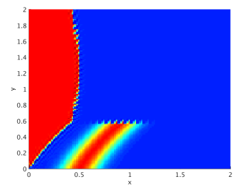
(a) $u^{k}$ at $k=16$

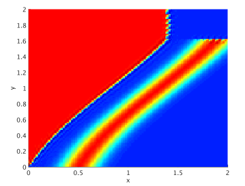
(b) $u^{k}$ at $k=48$

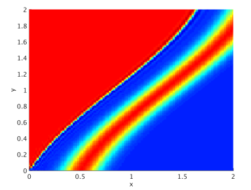
(c) $u^{k}$ at $k=64$

Figure 1: Evolution of the iterative solution for the 2D transport equation using the iHDG-II algorithm.

Table 1: The number of iterations taken by the iHDG-II algorithm for the transport equation in 2D and 3D settings.

$N_{el}$(2D)	$N_{el}$(3D)	$p$	2D solution	3D solution
4x4	2x2x2	1	9	6
8x8	4x4x4	1	17	12
16x16	8x8x8	1	33	23
32x32	16x16x16	1	65	47
4x4	2x2x2	2	9	6
8x8	4x4x4	2	17	12
16x16	8x8x8	2	33	23
32x32	16x16x16	2	65	47
4x4	2x2x2	3	9	7
8x8	4x4x4	3	17	12
16x16	8x8x8	3	33	23
32x32	16x16x16	3	65	47
4x4	2x2x2	4	9	6
8x8	4x4x4	4	17	12
16x16	8x8x8	4	33	24
32x32	16x16x16	4	64	48

Table 2 shows strong scaling results for the 3D transport problem. The parallel efficiency is over $90\%$ for all the cases except for the case where we use 16,384 cores and 16 elements per core whose efficiency is $59\%$. This is due to the fact that, with 16 elements per core, the communication cost dominates the computation. Table 3 shows the weak scaling with 1024 and 128 elements/core. Since the number of iterations increases linearly with the number of elements, we can see a similar increase in time when we increase the number of elements, and hence cores.

Let us now consider the time dependent 3D transport equation with the following exact solution

$$u^{e}=e^{-5((x-0.35t)^{2}+(y-0.35t)^{2}+(z-0.35t)^{2})},$$

where the velocity field is chosen to be $\boldsymbol{\beta}=(0.2,0.2,0.2)$. In Figure 2 are the numbers of iHDG iterations taken per time step to converge versus the $CFL$ number. As can be seen, for $CFL$ in the range $\left[1,5\right]$ the number of iterations grows mildly. As a result, we get a much better weak scaling results in Table 4 in comparison to the steady state case in Table 3.

Table 2: Strong scaling results on TACC’s Stampede system for the 3D transport problem.

$N_{el}=262,144$, $p=4$, dof=32.768 million, Iterations=190
#cores	time [s]	$N_{el}$/core	efficiency [%]
64	1758.62	4096	100.0
128	883.88	2048	99.5
256	439.94	1024	99.9
512	228.69	512	96.1
1024	113.87	256	96.5
2048	56.36	128	97.5
4096	29.26	64	91.8
16384	11.38	16	59
$N_{el}=2,097,152$, $p=4$, dof=262.144 million, Iterations=382
#cores	time [s]	$N_{el}$/core	efficiency [%]
512	3634.89	4096	100.0
1024	1788.78	2048	101.5
2048	932.495	1024	97.3
4096	447.337	512	101.5
8192	232.019	256	97.9
16384	117.985	128	92.9

Table 3: Weak scaling results on TACC’s Stampede system for the 3D transport problem.

1024 $N_{el}$/core, $p=4$
#cores	time [s]	time ratio	Iterations ratio
4	103.93	1	1
32	217.23	2.1	2
256	439.94	4.2	4
2048	932.49	8.9	8
128 $N_{el}$/core, $p=4$
#cores	time [s]	time ratio	Iterations ratio
4	6.52	1	1
32	13.68	2.1	2
256	27.71	4.2	4
2048	56.37	8.6	8

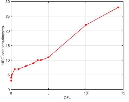
Figure 2: CFL versus Iterations for the 3D time dependent transport

Table 4: Weak scaling results on TACC’s Stampede system for the 3D time dependent transport problem.

128 $N_{el}$/core, ${p}=4$, $\Delta t$=0.01, $|\boldsymbol{\beta}|_{max}$=0.35
#cores	time/timestep [s]	time ratio	Iterations ratio	CFL
4	1.69	1	1	0.45
32	1.91	1.1	1.1	0.9
256	2.09	1.2	1.1	1.8
2048	2.72	1.6	1.4	3.6
16384	4.68	2.8	2.1	7.2

6.2 Linearized shallow water equations

The goal of this section is to verify the theoretical findings in section 4.4. To that extent, let us consider equation (21) with a linear standing wave, for which, $\Phi=1$, $f=0$, $\gamma=0$ (zero bottom friction), ${\boldsymbol{\tau}}=0$ (zero wind stress). The domain is $[0,1]\times[0,1]$ and the wall boundary condition is applied on the domain boundary. The following exact solution [62] is taken

$$\phi^{e} =\cos(\pi x)\cos(\pi y)\cos(\sqrt{2}\pi t),$$ (50a)

$$u^{e} =\frac{1}{\sqrt{2}}\sin(\pi x)\cos(\pi y)\sin(\sqrt{2}\pi t),$$ (50b)

$$v^{e} =\frac{1}{\sqrt{2}}\cos(\pi x)\sin(\pi y)\sin(\sqrt{2}\pi t).$$ (50c)

We use Crank-Nicolson method for the temporal discretization and the iHDG-II approach for the spatial discretization. In Table 5 we compare the number of iterations taken by iHDG-I and iHDG-II methods for two different time steps $\Delta t=0.1$ and $\Delta t=0.01$. Here, “$*$” indicates divergence. As can be seen from the third and fourth columns, the iHDG-I method diverges for finer meshes and/or larger time steps. This is consistent with the findings in section 4.4 where the divergence is expected because of the lack of mesh independent stability in the velocity. On the contrary, iHDG-II converges for all cases.

Table 5: Comparison of iHDG-I and iHDG-II for the shallow water equations.

$N_{el}$	$p$	iHDG-I		iHDG-II
		$\Delta t=10^{-1}$	$\Delta t=10^{-2}$	$\Delta t=10^{-1}$	$\Delta t=10^{-2}$
16	1	19	6	14	6
64	1	*	6	18	9
256	1	*	7	32	10
1024	1	*	9	59	8
16	2	*	9	15	9
64	2	*	11	19	9
256	2	*	13	32	11
1024	2	*	15	59	12
16	3	*	7	16	8
64	3	*	9	20	8
256	3	*	12	31	10
1024	3	*	*	59	12
16	4	*	10	17	9
64	4	*	12	32	10
256	4	*	*	60	9
1024	4	*	*	112	13

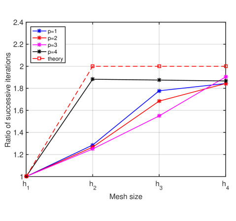
${p}$	iHDG-II				Asymptotics
	$h_{1}$	$h_{2}$	$h_{3}$	$h_{4}$
$2$	1.07	1.06	1	1	2
$3$	1.14	1.11	0.97	1	3.33
$4$	1.21	1.78	1.87	1.9	5

Figure 3: Growth of iterations with mesh size $h$ (left) and solution order $p$ (right) for the iHDG-II method for the shallow water equation.

In Table 5, we use a series of structured quadrilateral meshes with uniform refinements such that the ratio of successive mesh sizes is $1/2$. The asymptotic result (35), which is valid for $\frac{h}{\Delta t(p+1)(p+2)\sqrt{\Phi}}\ll 1$, predicts that the ratio of the number of iterations required by successive refined meshes is $2$, and the results in Figure 3 confirm this prediction. The last two columns of Table 5 also confirms the asymptotic result (35) that the number of iHDG-II iterations scales linearly with the time stepsize.

Next, we study the iHDG iteration growth as the solution order $p$ increases. The asymptotic result (35) predicts that $k={O}(p^{2})$. In Table 3, rows 2–4 show the ratio of the number of iterations taken for solution orders $p=\left\{2,3,4\right\}$ over the one for $p=1$ for four different meshsizes as in Table 5. As can be seen, the theoretical estimation is conservative.

6.3 Convection-diffusion equation

In this section the following exact solution for equation (38) is considered

$$u^{e}=\frac{1}{\pi}\sin(\pi x)\cos(\pi y)\sin(\pi z).$$

The forcing is chosen such that it corresponds to the exact solution. The velocity field is chosen as $\boldsymbol{\beta}=(1+z,1+x,1+y)$ and we take $\nu=1$. The domain is $[0,1]\times[0,1]\times[0,1]$. A structured hexahedral mesh is used for the simulations. The stopping criteria based on the exact solution is used as in the previous sections.

In Table 6 we report the number of iterations taken by iHDG-I and iHDG-II methods for different values of the diffusion coefficent $\kappa$. Similar to the shallow water equations, due to the lack of stability in ${\boldsymbol{{\sigma}}}$, iHDG-I diverges when $\kappa$ is large for fine meshes and/or high solution orders. The iHDG-II method, on the other hand, converges for all the meshes and solution orders, and the number of iterations are smaller than that of the iHDG-I method. Next, we verify the growth of iHDG-II iterations predicted by the asymptotic result (47).

Since $\min\left\{\kappa^{-1},\lambda\right\}=\lambda$ for all the numerical results considered here, due to (47) we expect the number of iHDG-II iterations to be independent of $\kappa$ and this can be verified in Table 6. In Figure 4 the growth of iterations with respect to mesh size $h$ for different $\kappa$ are compared. In the asymptotic limit, for all the cases, the ratio of successive iterations reaches a value of around $1.7$ which is close to the theoretical prediction $2$. Hence the theoretical analysis predicts well the growth of iterations with respect to the mesh size $h$. On the other hand, columns $6-8$ in Table 6 show that the iterations are almost independent of solution orders. This is not predicted by the theoretical results which indicates that the number of iterations scales like $\mathcal{O}(p^{2})$. The reason is due to the convection dominated nature of the problem, for which we have shown that the number of iterations is independent of the solution order.

Finally, we consider the elliptic regime with $\kappa=1$ and $\boldsymbol{\beta}=0$. For this case we use the following stopping criteria based on the direct solver solution $u_{direct}$

$$\left\|u^{k}-u_{direct}\right\|_{L^{2}}<10^{-10}.$$

As shown in Figure 5, our theoretical analysis predicts well the relation between the number of iterations and the mesh size and the solution order.

Table 6: Comparison of iHDG-I and iHDG-II methods for different $\kappa$.

$h$	$p$	iHDG-I			iHDG-II
		$\kappa=10^{-2}$	$\kappa=10^{-3}$	$\kappa=10^{-6}$	$\kappa=10^{-2}$	$\kappa=10^{-3}$	$\kappa=10^{-6}$
0.5	1	24	23	23	17	17	17
0.25	1	30	34	35	25	25	26
0.125	1	50	55	56	35	37	38
0.0625	1	90	94	97	62	64	65
0.5	2	26	24	25	17	19	19
0.25	2	41	42	42	27	27	27
0.125	2	66	67	67	42	43	43
0.0625	2	*	109	110	67	70	71
0.5	3	27	31	31	19	19	19
0.25	3	33	33	38	24	26	27
0.125	3	*	58	60	38	39	41
0.0625	3	*	102	106	69	69	71
0.5	4	26	27	27	17	19	19
0.25	4	50	41	43	26	27	27
0.125	4	*	71	72	42	45	46
0.0625	4	*	123	125	73	78	79

(a) $\kappa=10^{-2}$

(b) $\kappa=10^{-3}$

(c) $\kappa=10^{-6}$

Figure 4: Ratio of successive iterations as we refine the mesh for the iHDG-II method for different $\kappa$.

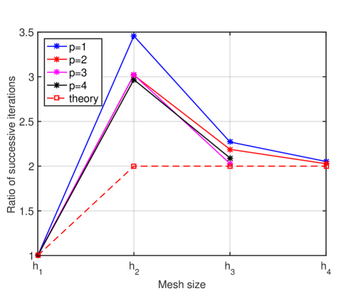
${p}$	iHDG-II			Asymptotics
	$h_{1}$	$h_{2}$	$h_{3}$
$2$	2.41	2.11	2.03	2
$3$	4.07	3.55	3.17	3.33
$4$	6.09	5.23	4.81	5

Figure 5: Growth of iterations with mesh size $h$ (left) and solution order $p$ (right) for the iHDG-II method for the elliptic equation.

7 Conclusions

We have presented an iterative HDG approach which improves upon our previous work [45] in several aspects. In particular, it converges in a finite number of iterations for the scalar transport equation and is unconditionally convergent for both the linearized shallow water system and the convection-diffusion equation. Moreover, compared to our previous work [45], we provide several additional findings: 1) we make a connection between iHDG and the parareal method, which reveals interesting similarities and differences between the two methods; 2) we show that iHDG can be considered as a locally implicit method, and hence being somewhat in between fully explicit and fully implicit approaches; 3) for both the linearized shallow water system and the convection-diffusion equation, using an asymptotic approximation, we uncover a relationship between the number of iterations and time stepsize, solution order, meshsize and the equation parameters. This allows us to choose the time stepsize such that the number of iterations is approximately independent of the solution order and the meshsize; 4) we show that iHDG-II has improved stability and convergence rates over iHDG-I; and 5) we provide both strong and weak scalings of our iHDG approach up to $16,384$ cores. Ongoing work is to develop a preconditioner to reduce the number of iterations as the mesh is refined. Equally important is to exploit the iHDG approach with small number of iterations as a preconditioner.

Appendix A. Proof of well-posedness of local solver of the iHDG-II method for the convection-diffusion equation

Proof.

Choosing ${\boldsymbol{{\sigma}}}^{k+1}$ and $u^{k+1}$ as test functions in (40a)-(40), integrating the second term in (40a) by parts, using (12) for second term in (40), and then summing up the resulting two equations we obtain

$$\kappa^{-1}\left({\boldsymbol{{\sigma}}}^{k+1},{\boldsymbol{{\sigma}}}^{k+1}\right)_{K}+\left(\left\{\nu-\frac{\nabla\cdot\boldsymbol{\beta}}{2}\right\}u^{k+1},u^{k+1}\right)_{K}\\ +\left<\left(\frac{\boldsymbol{\beta}\cdot{\bf n}}{2}+\tau\right)u^{k+1},u^{k+1}\right>_{\partial K}+\left<({\boldsymbol{{\sigma}}}^{k+1}\cdot{\bf n}-\tau u^{k+1}),{\hat{u}}^{k,k+1}\right>_{\partial K}=0.$$ (51)

Substituting (41) in the above equation and simplifying some terms we get,

$$\sum_{K}\kappa^{-1}\left\|\left({\boldsymbol{{\sigma}}}^{k+1}\right)^{-}\right\|_{K}^{2}+\left(\left\{\nu-\frac{\nabla\cdot\boldsymbol{\beta}}{2}\right\}\left(u^{k+1}\right)^{-},\left(u^{k+1}\right)^{-}\right)_{K}$$

$$+\left<\left\{\frac{|\boldsymbol{\beta}\cdot\mathbf{n}|^{2}+2}{2\alpha}\right\}\left(u^{k+1}\right)^{-},\left(u^{k+1}\right)^{-}\right>_{\partial K}+\left<\frac{1}{\alpha}\left({\boldsymbol{{\sigma}}}^{k+1}\cdot\mathbf{n}\right)^{-},\left({\boldsymbol{{\sigma}}}^{k+1}\cdot\mathbf{n}\right)^{-}\right>_{\partial K}$$

$$+\left<\frac{\boldsymbol{\beta}\cdot\mathbf{n}^{-}}{\alpha}\left(u^{k+1}\right)^{-},\left({\boldsymbol{{\sigma}}}^{k+1}\cdot\mathbf{n}\right)^{-}\right>_{\partial K}=\sum_{\partial K}-\left<\frac{1}{\alpha}\left({\boldsymbol{{\sigma}}}^{k+1}\cdot\mathbf{n}\right)^{-},\left({\boldsymbol{{\sigma}}}^{k}\cdot\mathbf{n}\right)^{+}\right>_{\partial K}$$

$$-\left<\left\{\frac{\boldsymbol{\beta}\cdot\mathbf{n}^{+}+\tau^{+}}{\alpha}\right\}\left({\boldsymbol{{\sigma}}}^{k+1}\cdot\mathbf{n}\right)^{-},\left(u^{k}\right)^{+}\right>_{\partial K}+\left<\frac{\tau^{-}}{\alpha}\left(u^{k+1}\right)^{-},\left({\boldsymbol{{\sigma}}}^{k}\cdot\mathbf{n}\right)^{+}\right>_{\partial K}$$

$$+\left<\left\{\frac{\tau^{-}(\boldsymbol{\beta}\cdot\mathbf{n}^{+}+\tau^{+})}{\alpha}\right\}\left(u^{k+1}\right)^{-},\left(u^{k}\right)^{+}\right>_{\partial K}.$$ (52)

Using the identity

$$\left<\frac{\boldsymbol{\beta}\cdot\mathbf{n}}{\alpha}u^{k+1},{\boldsymbol{{\sigma}}}^{k+1}\cdot\mathbf{n}\right>_{\partial K}=\left\|\frac{1}{\sqrt{2\alpha}}\left(\boldsymbol{\beta}\cdot\mathbf{n}u^{k+1}+{\boldsymbol{{\sigma}}}^{k+1}\cdot\mathbf{n}\right)\right\|_{\partial K}^{2}\\ -\left<\frac{\boldsymbol{\beta}\cdot\mathbf{n}^{2}}{2\alpha}u^{k+1},u^{k+1}\right>_{\partial K}-\left<\frac{1}{2\alpha}{\boldsymbol{{\sigma}}}^{k+1}\cdot\mathbf{n},{\boldsymbol{{\sigma}}}^{k+1}\cdot\mathbf{n}\right>_{\partial K},$$ (53)

and the coercivity condition (39) we can write (52) as

$$\sum_{K}\kappa^{-1}\left\|\left({\boldsymbol{{\sigma}}}^{k+1}\right)^{-}\right\|_{K}^{2}+\lambda\left\|\left(u^{k+1}\right)^{-}\right\|_{K}^{2}+\left\|\left(u^{k+1}\right)^{-}\right\|_{1/\alpha,{\partial K}}^{2}$$

$$+\left\|\left({\boldsymbol{{\sigma}}}^{k+1}\cdot\mathbf{n}\right)^{-}\right\|_{1/2\alpha,{\partial K}}^{2}+\left\|\frac{1}{\sqrt{2\alpha}}\left\{\boldsymbol{\beta}\cdot\mathbf{n}^{-}\left(u^{k+1}\right)^{-}+\left({\boldsymbol{{\sigma}}}^{k+1}\cdot\mathbf{n}\right)^{-}\right\}\right\|_{\partial K}^{2}\leq$$

$$\sum_{\partial K}-\left<\frac{1}{\alpha}\left({\boldsymbol{{\sigma}}}^{k+1}\cdot\mathbf{n}\right)^{-},\left({\boldsymbol{{\sigma}}}^{k}\cdot\mathbf{n}\right)^{+}\right>_{\partial K}-\left<\left\{\frac{\boldsymbol{\beta}\cdot\mathbf{n}^{+}+\tau^{+}}{\alpha}\right\}\left({\boldsymbol{{\sigma}}}^{k+1}\cdot\mathbf{n}\right)^{-},\left(u^{k}\right)^{+}\right>_{\partial K}$$

$$+\left<\frac{\tau^{-}}{\alpha}\left(u^{k+1}\right)^{-},\left({\boldsymbol{{\sigma}}}^{k}\cdot\mathbf{n}\right)^{+}\right>_{\partial K}+\left<\left\{\frac{\tau^{-}(\boldsymbol{\beta}\cdot\mathbf{n}^{+}+\tau^{+})}{\alpha}\right\}\left(u^{k+1}\right)^{-},\left(u^{k}\right)^{+}\right>_{\partial K}.$$ (54)

Since all the terms on the left hand side are positive, when we take the “forcing” to the local solver $\left\{\left(u^{k}\right)^{+},\left({\boldsymbol{{\sigma}}}^{k}\right)^{+}\right\}=\left\{0,{\bf 0}\right\}$, the only solution possible is $\left\{\left(u^{k+1}\right)^{-},\left({\boldsymbol{{\sigma}}}^{k+1}\right)^{-}\right\}=\left\{0,{\bf 0}\right\}$ and hence the method is well-posed. ∎

Appendix B. Proof of convergence of the iHDG-II method for the convection-diffusion equation

Proof.

In equation (54) omitting the last term on the left hand side and using Cauchy-Schwarz and Young’s inequalities for the terms on the right hand side we get

$$\sum_{K}\kappa^{-1}\left\|\left({\boldsymbol{{\sigma}}}^{k+1}\right)^{-}\right\|_{K}^{2}+\lambda\left\|\left(u^{k+1}\right)^{-}\right\|_{K}^{2}+\left\|\left(u^{k+1}\right)^{-}\right\|_{1/\alpha,{\partial K}}^{2}$$

$$+\left\|\left({\boldsymbol{{\sigma}}}^{k+1}\cdot\mathbf{n}\right)^{-}\right\|_{1/2\alpha,{\partial K}}^{2}\leq\sum_{\partial K}\frac{1}{2\varepsilon}\left<\left\{\frac{\tau^{-}+1}{\alpha}\right\}\left({\boldsymbol{{\sigma}}}^{k}\cdot\mathbf{n}\right)^{+},\left({\boldsymbol{{\sigma}}}^{k}\cdot\mathbf{n}\right)^{+}\right>_{\partial K}$$

$$+\frac{1}{2\varepsilon}\left<\left\{\frac{(1+\tau^{-})(\boldsymbol{\beta}\cdot\mathbf{n}^{+}+\tau^{+})}{\alpha}\right\}\left(u^{k}\right)^{+},\left(u^{k}\right)^{+}\right>_{\partial K}$$

$$+\frac{\varepsilon}{2}\left<\left\{\frac{1+\tau^{+}+\boldsymbol{\beta}\cdot\mathbf{n}^{+}}{\alpha}\right\}\left({\boldsymbol{{\sigma}}}^{k+1}\cdot\mathbf{n}\right)^{-},\left({\boldsymbol{{\sigma}}}^{k+1}\cdot\mathbf{n}\right)^{-}\right>_{\partial K}$$

$$+\frac{\varepsilon}{2}\left<\left\{\frac{\tau^{-}(1+\tau^{+}+\boldsymbol{\beta}\cdot\mathbf{n}^{+})}{\alpha}\right\}\left(u^{k+1}\right)^{-},\left(u^{k+1}\right)^{-}\right>_{\partial K}.$$ (55)

We can write the above inequality as

$$\kappa^{-1}\left\|\left({\boldsymbol{{\sigma}}}^{k+1}\right)^{-}\right\|_{K}^{2}+\lambda\left\|\left(u^{k+1}\right)^{-}\right\|_{K}^{2}+\frac{1}{\bar{\alpha}}\left\|\left(u^{k+1}\right)^{-}\right\|_{{\partial K}}^{2}+\frac{1}{2\bar{\alpha}}\left\|\left({\boldsymbol{{\sigma}}}^{k+1}\cdot\mathbf{n}\right)^{-}\right\|_{{\partial K}}^{2}$$

$$\leq\frac{\bar{\tau}+1}{2\varepsilon\alpha_{*}}\left\|\left({\boldsymbol{{\sigma}}}^{k}\cdot\mathbf{n}\right)^{+}\right\|_{\partial K}^{2}+\frac{(1+\bar{\tau})(\|\boldsymbol{\beta}\cdot\mathbf{n}\|_{L^{\infty}({\partial K})}+\bar{\tau})}{2\varepsilon\alpha_{*}}\left\|\left(u^{k}\right)^{+}\right\|_{\partial K}^{2}$$

$$+\frac{\varepsilon(1+\bar{\tau}+\|\boldsymbol{\beta}\cdot\mathbf{n}\|_{L^{\infty}({\partial K})})}{2\alpha_{*}}\left\|\left({\boldsymbol{{\sigma}}}^{k+1}\cdot\mathbf{n}\right)^{-}\right\|_{\partial K}^{2}$$

$$+\frac{\varepsilon\bar{\tau}(1+\bar{\tau}+\|\boldsymbol{\beta}\cdot\mathbf{n}\|_{L^{\infty}({\partial K})})}{2\alpha_{*}}\left\|\left(u^{k+1}\right)^{-}\right\|_{\partial K}^{2},$$ (56)

where $\bar{\tau}:=\|\tau\|_{L^{\infty}(\partial\Omega_{h})}$, $\bar{\alpha}:=\|\alpha\|_{L^{\infty}(\partial\Omega_{h})}$, and $\alpha_{*}:=\inf\limits_{{\partial K}\in\partial\Omega_{h}}\alpha$.

By the inverse trace inequality (29) we infer from (56) that

$$\sum_{\partial K}\mathcal{B}_{1}\left\|\left({\boldsymbol{{\sigma}}}^{k+1}\cdot\mathbf{n}\right)^{-}\right\|_{{\partial K}}^{2}+\mathcal{B}_{2}\left\|\left(u^{k+1}\right)^{-}\right\|_{{\partial K}}^{2}\\ \leq\sum_{\partial K}\left[\mathcal{C}_{1}\left\|\left(u^{k}\right)^{+}\right\|_{{\partial K}}^{2}+\mathcal{C}_{2}\left\|\left({\boldsymbol{{\sigma}}}^{k}\cdot\mathbf{n}\right)^{+}\right\|_{{\partial K}}^{2}\right],$$ (57)

which implies

$$\left\|\left({\boldsymbol{{\sigma}}}^{k+1}\cdot\mathbf{n},u^{k+1}\right)\right\|^{2}_{\mathcal{E}_{h}}\leq\mathcal{D}\left\|\left({\boldsymbol{{\sigma}}}^{k}\cdot\mathbf{n},u^{k}\right)\right\|^{2}_{\mathcal{E}_{h}},$$

where the constant $\mathcal{D}$ is computed as in (44). Therefore

$$\left\|\left({\boldsymbol{{\sigma}}}^{k+1}\cdot\mathbf{n},u^{k+1}\right)\right\|^{2}_{\mathcal{E}_{h}}\leq\mathcal{D}^{k+1}\left\|\left({\boldsymbol{{\sigma}}}^{0}\cdot\mathbf{n},u^{0}\right)\right\|^{2}_{\mathcal{E}_{h}}.$$ (58)

Inequalities (56) and (58) imply

$$\left\|\left({\boldsymbol{{\sigma}}}^{k+1},u^{k+1}\right)\right\|^{2}_{\Omega_{h}}\leq(\mathcal{E}\mathcal{D}+\mathcal{F})\mathcal{D}^{k}\left\|\left({\boldsymbol{{\sigma}}}^{0}\cdot\mathbf{n},u^{0}\right)\right\|^{2}_{\mathcal{E}_{h}},$$

and this concludes the proof.

∎

References

References

• [1] W. H. Reed, T. R. Hill, Triangular mesh methods for the neutron transport equation, Tech. Rep. LA-UR-73-479, Los Alamos Scientific Laboratory (1973).
• [2] P. LeSaint, P. A. Raviart, On a finite element method for solving the neutron transport equation, in: C. de Boor (Ed.), Mathematical Aspects of Finite Element Methods in Partial Differential Equations, Academic Press, 1974, pp. 89–145.
• [3] C. Johnson, J. Pitkäranta, An analysis of the discontinuous Galerkin method for a scalar hyperbolic equation, Mathematics of Computation 46 (173) (1986) 1–26.
• [4] J. Douglas, T. Dupont, Interior penalty procedures for elliptic and parabolic galerkin methods, Computing methods in applied sciences (1976) 207–216.
• [5] M. F. Wheeler, An elliptic collocation-finite element method with interior penalties, SIAM Journal on Numerical Analysis 15 (1) (1978) 152–161.
• [6] D. N. Arnold, An interior penalty finite element method with discontinuous elements, SIAM journal on numerical analysis 19 (4) (1982) 742–760.
• [7] B. Cockburn, G. E. Karniadakis, C.-W. Shu, Discontinuous Galerkin Methods: Theory, Computation and Applications, Lecture Notes in Computational Science and Engineering, Vol. 11, Springer Verlag, Berlin, Heidelberg, New York, 2000.
• [8] D. N. Arnold, F. Brezzi, B. Cockburn, L. D. Marini, Unified analysis of discontinuous galerkin methods for elliptic problems, SIAM journal on numerical analysis 39 (5) (2002) 1749–1779.
• [9] B. Cockburn, J. Gopalakrishnan, R. Lazarov, Unified hybridization of discontinuous Galerkin, mixed, and continuous Galerkin methods for second order elliptic problems, SIAM J. Numer. Anal. 47 (2009) 1319–1365.
• [10] B. Cockburn, J. Gopalakrishnan, F.-J. Sayas, A projection-based error analysis of HDG methods, Mathematics Of Computation 79 (271) (2010) 1351–1367.
• [11] R. M. Kirby, S. J. Sherwin, B. Cockburn, To CG or to HDG: A comparative study, J. Sci. Comput. 51 (2012) 183–212.
• [12] N. C. Nguyen, J. Peraire, B. Cockburn, An implicit high-order hybridizable discontinuous Galerkin method for linear convection-diffusion equations, Journal Computational Physics 228 (2009) 3232–3254.
• [13] B. Cockburn, B. Dong, J. Guzman, M. Restelli, R. Sacco, A hybridizable discontinuous Galerkin method for steady state convection-diffusion-reaction problems, SIAM J. Sci. Comput. 31 (2009) 3827–3846.
• [14] H. Egger, J. Schoberl, A hybrid mixed discontinuous Galerkin finite element method for convection-diffusion problems, IMA Journal of Numerical Analysis 30 (2010) 1206–1234.
• [15] B. Cockburn, J. Gopalakrishnan, The derivation of hybridizable discontinuous Galerkin methods for Stokes flow, SIAM J. Numer. Anal 47 (2) (2009) 1092–1125.
• [16] N. C. Nguyen, J. Peraire, B. Cockburn, A hybridizable discontinous Galerkin method for Stokes flow, Comput Method Appl. Mech. Eng. 199 (2010) 582–597.
• [17] N. C. Nguyen, J. Peraire, B. Cockburn, An implicit high-order hybridizable discontinuous Galerkin method for the incompressible Navier-Stokes equations, Journal Computational Physics 230 (2011) 1147–1170.
• [18] D. Moro, N. C. Nguyen, J. Peraire, Navier-Stokes solution using hybridizable discontinuous Galerkin methods, American Institute of Aeronautics and Astronautics 2011-3407.
• [19] N. C. Nguyen, J. Peraire, B. Cockburn, Hybridizable discontinuous Galerkin method for the time harmonic Maxwell’s equations, Journal Computational Physics 230 (2011) 7151–7175.
• [20] L. Li, S. Lanteri, R. Perrrussel, A hybridizable discontinuous Galerkin method for solving 3D time harmonic Maxwell’s equations, in: Numerical Mathematics and Advanced Applications 2011, Springer, 2013, pp. 119–128.
• [21] N. C. Nguyen, J. Peraire, B. Cockburn, High-order implicit hybridizable discontinuous Galerkin method for acoustics and elastodynamics, Journal Computational Physics 230 (2011) 3695–3718.
• [22] R. Griesmaier, P. Monk, Error analysis for a hybridizable discontinous Galerkin method for the Helmholtz equation, J. Sci. Comput. 49 (2011) 291–310.
• [23] J. Cui, W. Zhang, An analysis of HDG methods for the Helmholtz equation, IMA J. Numer. Anal. 34 (1) (2014) 279–295.
• [24] T. Bui-Thanh, From Godunov to a unified hybridized discontinuous Galerkin framework for partial differential equations, Journal of Computational Physics 295 (2015) 114–146.
• [25] T. Bui-Thanh, From Rankine-Hugoniot Condition to a Constructive Derivation of HDG Methods, Lecture Notes in Computational Sciences and Engineering, Springer, 2015, pp. 483–491.
• [26] T. Bui-Thanh, Construction and analysis of HDG methods for linearized shallow water equations, SIAM Journal on Scientific Computing 38 (6) (2016) A3696–A3719.
• [27] J. Wang, X. Ye, A weak galerkin finite element method for second-order elliptic problems, J. Comput. Appl. Math. 241 (2013) 103–115.
• [28] J. Wang, X. Ye, A weak Galerkin mixed finite element method for second order elliptic problems, Math. Comp. 83 (2014) 2101–2126.
• [29] Q. Zhai, R. Zhang, X. Wang, A hybridized weak galerkin finite element scheme for the stokes equations, Science China Mathematics (2015) 1–18.
• [30] L. Mu, J. Wang, X. Ye, A new weak galerkin finite element method for the helmholtz equation, IMA Journal of Numerical Analysis.
• [31] J. Brown, Efficient nonlinear solvers for nodal high-order finite elements in 3D, Journal of Scientific Computing 45 (1-3) (2010) 48–63.
• [32] A. Crivellini, F. Bassi, An implicit matrix-free discontinuous galerkin solver for viscous and turbulent aerodynamic simulations, Computers & Fluids 50 (1) (2011) 81–93.
• [33] D. A. Knoll, D. E. Keyes, Jacobian-free newton–krylov methods: a survey of approaches and applications, Journal of Computational Physics 193 (2) (2004) 357–397.
• [34] P.-L. Lions, On the Schwarz alternating method. I, in: First International Symposium on Domain Decomposition Methods for Partial Differential Equations (Paris, 1987), SIAM, Philadelphia, PA, 1988, pp. 1–42.
• [35] P.-L. Lions, On the Schwarz alternating method. II. Stochastic interpretation and order properties, in: Domain decomposition methods (Los Angeles, CA, 1988), SIAM, Philadelphia, PA, 1989, pp. 47–70.
• [36] P.-L. Lions, On the Schwarz alternating method. III. A variant for nonoverlapping subdomains, in: Third International Symposium on Domain Decomposition Methods for Partial Differential Equations (Houston, TX, 1989), SIAM, Philadelphia, PA, 1990, pp. 202–223.
• [37] L. Halpern, Optimized Schwarz waveform relaxation: roots, blossoms and fruits, in: Domain decomposition methods in science and engineering XVIII, Vol. 70 of Lect. Notes Comput. Sci. Eng., Springer, Berlin, 2009, pp. 225–232.
• [38] M. J. Gander, L. Gouarin, L. Halpern, Optimized Schwarz waveform relaxation methods: a large scale numerical study, in: Domain decomposition methods in science and engineering XIX, Vol. 78 of Lect. Notes Comput. Sci. Eng., Springer, Heidelberg, 2011, pp. 261–268.
• [39] M. J. Gander, S. Hajian, Analysis of Schwarz methods for a hybridizable discontinuous Galerkin discretization, SIAM J. Numer. Anal. 53 (1) (2015) 573–597.
• [40] M.-B. Tran, Parallel Schwarz waveform relaxation method for a semilinear heat equation in a cylindrical domain, C. R. Math. Acad. Sci. Paris 348 (13-14) (2010) 795–799.
• [41] M.-B. Tran, A parallel four step domain decomposition scheme for coupled forward–backward stochastic differential equations, Journal de mathématiques pures et appliquées 96 (4) (2011) 377–394.
• [42] M.-B. Tran, Overlapping domain decomposition: Convergence proofs, in: Domain Decomposition Methods in Science and Engineering XX, Springer, 2013, pp. 493–500.
• [43] M.-B. Tran, The behavior of domain decomposition methods when the overlapping length is large, Central European Journal of Mathematics 12 (10) (2014) 1602–1614.
• [44] B. Cockburn, O. Dubois, J. Gopalakrishnan, S. Tan, Multigrid for an HDG method, IMA Journal of Numerical Analysis (2013) 1–40.
• [45] S. Muralikrishnan, M.-B. Tran, T. Bui-Thanh, iHDG: An iterative HDG framework for partial differential equations, SIAM Journal on Scientific Computing 39 (5) (2017) S782–S808.
• [46] M. J. Gander, S. Hajian, Block jacobi for discontinuous galerkin discretizations: no ordinary schwarz methods, in: Domain Decomposition Methods in Science and Engineering XXI, Springer, 2014, pp. 305–313.
• [47] M. J. Gander, S. Hajian, Analysis of schwarz methods for a hybridizable discontinuous galerkin discretization: the many subdomain case, arXiv preprint arXiv:1603.04073.
• [48] K. O. Friedrichs, Symmetric positive linear differential equations, Communications on pure and applied mathematics XI (1958) 333–418.
• [49] M. J. Gander, Analysis of the parareal algorithm applied to hyperbolic problems using characteristics, Boletin de la Sociedad Espanola de Matemática Aplicada 42 (2008) 21–35.
• [50] Z. Kaczkowski, The method of finite space-time elements in dynamics of structures, Journal of Technical Physics 16 (1) (1975) 69–84.
• [51] J. Argyris, D. Scharpf, Finite elements in time and space, Nuclear Engineering and Design 10 (4) (1969) 456–464.
• [52] J. T. Oden, A general theory of finite elements. ii. applications, International Journal for Numerical Methods in Engineering 1 (3) (1969) 247–259.
• [53] C. M. Klaij, J. J. van der Vegt, H. van der Ven, Space–time discontinuous Galerkin method for the compressible Navier–Stokes equations, Journal of Computational Physics 217 (2) (2006) 589–611.
• [54] T. Ellis, J. Chan, L. Demkowicz, Robust DPG methods for transient convection-diffusion, in: Building Bridges: Connections and Challenges in Modern Approaches to Numerical Partial Differential Equations, Springer, 2016, pp. 179–203.
• [55] S. Rhebergen, B. Cockburn, A space–time hybridizable discontinuous galerkin method for incompressible flows on deforming domains, Journal of Computational Physics 231 (11) (2012) 4185–4204.
• [56] J.-L. Lions, Y. Maday, G. Turinici, Résolution d’edp par un schéma en temps pararéel, Comptes Rendus de l’Académie des Sciences-Series I-Mathematics 332 (7) (2001) 661–668.
• [57] I. Garrido, B. Lee, G. Fladmark, M. Espedal, Convergent iterative schemes for time parallelization, Mathematics of computation 75 (255) (2006) 1403–1428.
• [58] C. Farhat, M. Chandesris, Time-decomposed parallel time-integrators: theory and feasibility studies for uid, structure, and fluid-structure applications, International Journal for Numerical Methods in Engineering 58 (9) (2003) 1397–1434.
• [59] Y. Maday, G. Turinici, A parareal in time procedure for the control of partial differential equations, Comptes Rendus Mathematique 335 (4) (2002) 387–392.
• [60] M. Minion, A hybrid parareal spectral deferred corrections method, Communications in Applied Mathematics and Computational Science 5 (2) (2011) 265–301.
• [61] M. J. Gander, S. Vandewalle, Analysis of the parareal time-parallel time-integration method, SIAM Journal on Scientific Computing 29 (2) (2007) 556–578.
• [62] F. X. Giraldo, T. Warburton, A high-order triangular discontinous Galerkin oceanic shallow water model, International Journal For Numerical Methods In Fluids 56 (2008) 899–925.
• [63] J. Chan, Z. Wang, A. Modave, J.-F. Remacle, T. Warburton, GPU-accelerated discontinuous galerkin methods on hybrid meshes, Journal of Computational Physics 318 (2016) 142–168.
• [64] T. Warburton, J. S. Hesthaven, On the constants in $hp$-finite element trace inverse inequalities, Comput. Methods Appl. Mech. Engrg. 192 (25) (2003) 2765–2773.
• [65] M. Taylor, J. Tribbia, M. Iskandarani, The spectral element method for the shallow water equations on the sphere, Journal of Computational Physics 130 (1) (1997) 92 – 108.
• [66] L. C. Wilcox, G. Stadler, C. Burstedde, O. Ghattas, A high-order discontinuous Galerkin method for wave propagation through coupled elastic-acoustic media, Journal of Computational Physics 229 (24) (2010) 9373–9396.
• [67] C. Burstedde, O. Ghattas, M. Gurnis, T. Isaac, G. Stadler, T. Warburton, L. C. Wilcox, Extreme-scale AMR, in: SC10: Proceedings of the International Conference for High Performance Computing, Networking, Storage and Analysis, ACM/IEEE, 2010.
• [68] C. Burstedde, O. Ghattas, M. Gurnis, E. Tan, T. Tu, G. Stadler, L. C. Wilcox, S. Zhong, Scalable adaptive mantle convection simulation on petascale supercomputers, in: SC08: Proceedings of the International Conference for High Performance Computing, Networking, Storage and Analysis, ACM/IEEE, 2008.