Entanglement entropy of a three-spin interacting spin chain with a time-reversal breaking impurity at one boundary

Abstract

We investigate the effect of a time-reversal breaking impurity term (of strength $\lambda_{d}$) on both the equilibrium and non-equilibrium critical properties of entanglement entropy (EE) in a three-spin interacting transverse Ising model which can be mapped to a $p$-wave superconducting chain with next-nearest-neighbor hopping and interaction. Importantly, we find that the logarithmic scaling of the EE with block size remains unaffected by the application of the impurity term, although, the coefficient (i.e., central charge) varies logarithmically with the impurity strength for a lower range of $\lambda_{d}$ and eventually saturates with an exponential damping factor ($\sim\exp(-\lambda_{d})$) for the phase boundaries shared with the phase containing two Majorana edge modes. On the other hand, it receives a linear correction in term of $\lambda_{d}$ for an another phase boundary. Finally, we focus to study the effect of the impurity in the time evolution of the EE for the critical quenching case where impurity term is applied only to the final Hamiltonian. Interestingly, it has been shown that for all the phase boundaries, in contrary to the equilibrium case, the saturation value of the EE increases logarithmically with the strength of impurity in a certain regime of $\lambda_{d}$ and finally, for higher values of $\lambda_{d}$, it increases very slowly dictated by an exponential damping factor. The impurity induced behavior of EE might bear some deep underlying connection to thermalization.

I Introduction

Study of various quantum information theoretic measures such as fidelity gu08 , decoherence quan06 ; damski11a , concurrence wootters01 ; osterloh02 , quantum discord ollivier01 and entanglement entropy (EE) vidal03 has grabbed immense attention as it connects the quantum information science kitaev09 ; nag12b ; sachdeva14 ; suzuki15 ; nag15 ; nag16 ; rajak16 , statistical physics and condensed matter physics chakrabarti96 ; sachdev99 ; polkovnikov11 ; dutta15 in a concrete way. All of the above quantities are able to capture the ground state singularity and thus are used as indicators of quantum phase transition (QPT). For example, the EE of a block of length $l$ quantified by von Neumann entropy is given by

$$S(l)=-{\rm Tr}(\rho_{l}\ln\rho_{l}),$$ (1)

where the reduced density matrix $\rho_{l}={\rm Tr}_{L-l}(\rho)$ is obtained after tracing over the block of length $L-l$ from the composite system of length $L$ with pure state density matrix $\rho$. For a one-dimensional homogeneous critical spin chain with open boundary conditions, the EE scales with the shortest length scale ($l$) of the system as $S=\frac{c}{6}\ln l+\gamma$, where $c$ is a universal quantity and given by the central charge of the underlying conformal field theory, whereas $\gamma$ is a non-universal constant vidal03 ; calabrese04 . In the context of disordered spin chain (i.e., inhomogeneous case), for the critical case, it has been shown that the EE still varies logarithmically with block size but it acquires an effective central charge different from the bare central charge derived in the clean limit refael07 . It has been shown that the effective central charge also appears for the interface defects in a spin chain peschel05 .

At the same time, the study of entanglement spectrum and EE in quantum many-body systems has initiated a plethora of intensive research to characterize a topological system, through the concept of quantum entanglement li08 ; yao10 ; fidkowski10 ; pollmann10 ; facchi08 . The topological phases are charaterized by a topological invariant number (Chern number or $Z_{2}$ invariant or zero energy Majorana modes) and this phase supports edge modes hasan10 ; qi11 . In the connection of EE and edge state, it is noteworthy that the equilibrium EE receives a finite contribution from the localized boundary states in addition to the contribution from bulk energy spectrum. The finite contribution from boundaries is associated to the non-zero value of the Berry phase ryu06 . A non-extensive correction to the area law of EE, named as topological EE, has been proposed as a tool to characterize the topological phases of the systemkitaev06 . Interestingly, it has been shown for two dimension spin-orbit coupled superconductor that the derivatives of the EE with respect to model parameters are sharply peaked at the point of topological phase transitions borchmann14 .

In parallel, the behavior of the EE in quantum systems considering a non-equilibrium situation has received an enormous amount of attention in recent years  calabrese05 ; eisler07 ; calabrese07 ; eisler08 ; igloi09 ; hsu09 ; cardy11 . The upsurge of such studies is motivated by the experimental demonstration in optical lattice bloch08 . In particular, an out-of-equilibrium one-dimensional Bose gases has been prepared experimentally using the combination of a two-dimensional optical lattice and a crossed dipole trap kinoshita05 ; kinoshita06 . It has been shown that a global sudden quench leads to an initial linear rise of the EE with time followed by a saturation calabrese05 . Moreover, the dynamics of EE in the random transverse-field Ising chain after a sudden critical quench becomes ultraslow and has a double-logarithmic time dependence igloi12 . Also, the robustness of the Majorana zero-mode in the infinite time limit following a sudden quench of a one-dimensional p-wave superconductor has been investigated by examining the one-particle entanglement spectrum chung14 . The quench dynamics in optical lattice with $\rm Rb^{87}$ atoms is experimentally investigated in the context of quantum information namely, the signature of Lieb-Robinson bound of light-cone-like spreading of correlations is studied cheneau12 . Moreover, optical interferometry is directly used to measure entanglement entropy in a quantum many-body system composed of ultracold bosonic atoms in optical lattices islam15 .

In recent years, a considerable amount of work has been carried out to investigate the topological properties of one-dimensional $p$-wave Majorana chain kitaev01 ; fulga11 ; sau12 ; lutchyn11 ; degottardi11 ; degottardi13 ; thakurathi13 ; wdegottardi13 ; alicea12 ; rajak14 ; rajak14b . Our main aim here is to study the effect of a single impurity, located at one of the boundaries, on the critical behavior of the EE in this model with an additional next nearest neighbor hopping term. This single impurity indeed breaks the time-reversal invariance of the system. We show that in the equilibrium case, the derivative of EE can be used as an indicator of QPTs. We find that the scaling relation of the EE with the subsystem size remains same as obtained in the inhomogeneous case with an effective central charge. This effective central charge here shows a logarithmic scaling relation with $\lambda_{d}$ for an initial window of $\lambda_{d}$ and eventually saturates for large value of $\lambda_{d}$. This phenomena is observed at the phase boundaries shared with the phase containing two Majorana modes sitting at each end of the chain. On the other hand, for the phase boundary separating topological phase with one Majorana mode from non-topological one, the effective central charge acquires a linear correction due to this impurity term. Additionally, for the non-equilibrium time evolution of EE obtained by adding a boundary impurity term to the critical quenched chain, irrespective of the nature of phase boundaries the logarithmic behavior and the subsequent exponential scaling show up only in the saturation value of the EE but not in the initial rise of EE.

This paper is organized as follows: In Sec. II we introduce the three-spin interacting transverse field Ising model and discuss its phase diagram. We also mention the effect of an impurity term on the different phases of the model. In Sec. III, we present the method to compute EE and extend it to calculate the time-evolution of the EE numerically. In Sec. IV, we illustrate our results for equilibrium as well as for non-equilibrium case. Finally, we provide our concluding remarks in Sec. V.

II Model

The Hamiltonian we consider here is given by a three-spin interacting transverse Ising model with $N$ spins  kopp05

$$H~{}=~{}-\sum_{n}(h\sigma_{n}^{z}~{}+~{}\lambda_{1}\sigma_{n}^{x}\sigma_{n+1}^{x}~{}+~{}\lambda_{2}\sigma_{n-1}^{x}\sigma_{n}^{z}\sigma_{n+1}^{x}),$$ (2)

where $h$, $\lambda_{1}$ and $\lambda_{2}$ are transverse magnetic field, cooperative interaction and three-spin interaction respectively and, $\sigma^{\alpha}$ ($\alpha=x,y,z$) are the standard Pauli matrices. Using Jordan-Wigner transformation the model can be written in terms of spinless fermions with a next-nearest-neighbor hopping and superconducting pairing terms. At the same time, one can re-write the Hamiltonian in terms of Majorana fermions with open boundary condition (OBC), given by

$$H=-i\Big{[}-h\sum_{n=1}^{N}b_{n}a_{n}~{}+~{}\lambda_{1}\sum_{n=1}^{N-1}b_{n}a_{n+1}~{}+~{}\lambda_{2}\sum_{n=2}^{N-1}b_{n-1}a_{n+1}\Big{]}.$$ (3)

where, $a_{n}=c_{n}^{\dagger}+c_{n},b_{n}=-i(c_{n}^{\dagger}-c_{n})$ are Majorana fermions. The system discussed above has time-reversal symmetry ($T^{2}=1$). This transformation $T$ is defined as the complex conjugation of all the objects in the Hamiltonian (3). As a result, $T$ leads to $a_{n}\rightarrow a_{n}$ and $b_{n}\rightarrow-b_{n}$, and hence, Eq. (3) is invariant under time-reversal  wdegottardi13 .

We now briefly discuss the phase diagram of the model with $h=1$ (see Fig. (1)). This model has three phases: (i) the ferromagnetic phase which is topologically non-trivial hosting one unpaired Majorana at each end, i.e., $a_{1}$ and $b_{N}$, (ii) the paramagnetic phase, a non-topological phase, with no Majorana edge modes, and (iii) three-spin dominated topological phase with two unpaired Majorana modes at each edge i.e., $a_{1}$ and $a_{2}$ are at the left boundary with $b_{N}$ and $b_{N-1}$ exist at the right boundary. The detail of the model and phase diagram are discussed in Refs.niu12 ; rajak17 .

It is noteworthy that a similar kind of model namely, cluster-Ising model, has been studied before in the context of locating its QPTs between cluster and antiferromagnetic phases using geometric son11 and multipartite giampaolo14 entanglement. Although, the three-spin dominated phase of the model (2) is analogous to the cluster phase of the cluster-Ising model, there are a few differences between these two models: (i) model given in Eq. (2) contains an extra transverse field term, (ii) it has $Z_{2}^{T}$ symmetry (an anti-unitary $Z_{2}$ symmetry, $\sigma_{x}\rightarrow-\sigma_{x}$) friedman17 , whereas the cluster-Ising model is symmetric under is symmetric under $Z_{2}\times Z_{2}$, and (iii) the dual model of (2) is a transverse XY spin chain, on the other hand, the cluster-Ising model is its self-dual.

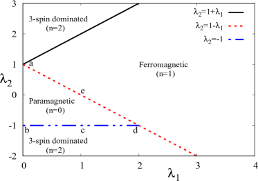
Figure 1: (Color online) Zero-temperature phase diagram of the model Hamiltonian (2) for $h=1$. The line $\lambda_{2}=1+\lambda_{1}$ represents the phase boundary between upper $3$-spin dominated phase (with two zero-energy Majorana end modes at each edge) and ferromagnetic phase with one Majorana at each end. There are two more phase boundaries, given by $\lambda_{2}=1-\lambda_{1}$ ($a-e-d$ line) and $\lambda_{2}=-1$ ($b-d$ line). The paramagnetic region denoted by $n=0$ does not have any zero-energy Majorana mode. In terms of topology both the $3$-spin dominated phases have two zero-energy Majorana modes at each end.

Our main goal is to find the effect of an impurity term in the critical behavior of the EE for both equilibrium and non-equilibrium cases. To achieve this goal, we introduce an additional term in the Hamiltonian (3) of the form rajak17

$$H_{\rm imp}~{}=~{}-i\lambda_{d}a_{j}a_{q},q=j+m.$$ (4)

The impurity term (4) affects the phase with two Majorana modes at one end (three-spin dominated phase). We here take into account the impurity term (4), located in the left edge of the system, that results in the annihilation of the $a$-type Majorana modes, however, the $b$-type Majorana modes residing at the right edge remain intact niu12 ; rajak17 . In contrast, the phase with one Majorana mode at each end remains unaffected. This term breaks the time-reversal symmetry of the system as $T$ reverses the sign of $H_{\rm imp}$. The annihilation of the edge Majorana mode is related to this symmetry breaking.

In the spin representation, the impurity Hamiltonian is expressed as $H_{\rm imp}=\lambda_{d}\sigma_{j}^{y}\prod_{n=j+1}^{j+m-1}(-\sigma_{n}^{z})\sigma_{j+m}^{x}$, which is a string operator. Therefore, in the spin language, the breaking of time reversal symmetry of the model in Eq. (3) is related to the breaking of $Z_{2}^{T}$ symmetry as the impurity term explicitly breaks this symmetry. Similarly for the cluster Ising model, we note that if one considers an additional impurity term, breaking $Z_{2}\times Z_{2}$ symmetry of the cluster phase, the existence of the edge Majorana modes might get affected in a similar fashion there also.

As mentioned already, the impurity term is a non-local string operator, though, in the Majorana language we can say it is quasi-local (see Eq. (4)). We hence stress that the impurity is purely quantum in nature. In parallel, the effect of a classical impurity, the zero transverse field at the first site of an otherwise homogeneous chain, has been investigated in a quantum Ising chain by studying the finite size scaling of the magnetizations apollaro17 . The nature of this impurity is classical due to the fact that the left most spin can not flip; in contrary, the impurity term considered in Eq. (4) is able to flip the spins. Simultaneously, transverse Ising model with multi-impurities gives rise to many non-trivial changes in deformation energy and specific heat huang15 .

Connecting to experimental realization, the impurity term in Eq. (4) can be prepared by experiments on entangled atoms in optical lattice. The array of parallel spin chains are created from two-dimensional degenerate gas of ${}^{87}{\rm Rb}$ atoms by applying two horizontal optical lattice beams. The atoms are initially prepared in a hyperfine state and then impurity is introduced by changing the hyperfine structure of one of the atoms fukuhara .

III Entanglement entropy

We shall here present our numerical method to calculate EE in the Majorana basis under the sudden quenching of a parameter of the chain. In order to formulate the non-equilibrium EE, we first briefly discuss the equilibrium EE in the Majorana basis latorre04 . Let us consider a general quadratic form of Eq. (3) in terms of Majorana operators

$$H=\frac{i}{4}\sum_{m,n=1}^{2N}e_{m}A_{mn}e_{n},$$ (5)

where $e_{2m-1}=a_{m}$ and $e_{2m}=b_{m}$. The matrix elements for $A$ are given by $A_{n,n+1}=-A_{n+1,n}=1$, $A_{2n,2n+1}=-A_{2n+1,2n}=-\lambda_{1}$ and $A_{2n,2n+3}=-A_{2n+3,2n}=-\lambda_{2}$. The impurity Hamiltonian (4) generates two extra elements in the matrix $A$: $A_{2j-1,2j+2m-1}=-A_{2j+2m-1,2j-1}=-\lambda_{d}$.

Let $W\in SO(2N)$ be a special orthogonal matrix that makes $A$ block diagonal of the form,

$$D=\bigoplus_{k=1}^{N}\tilde{\epsilon}_{k}\left[\begin{array}[]{cc}0&1\\ -1&0\end{array}\right],$$ (6)

where $D=WAW^{\dagger}$. Now, a new set of Majorana operators is defined as

$$d_{p}=\sum_{m=1}^{2N}W_{pm}e_{m},\hskip 5.69054pt{\rm where}\hskip 5.69054ptp=1,\cdots,2N.$$ (7)

Here, $d_{p}$ satisfies the relations $d_{p}^{\dagger}=d_{p},~{}\{d_{p},d_{q}\}=2\delta_{pq}$ The Hamiltonian in Eq. (5) in terms of the new Majorana operators is given by

$$H=\frac{i}{4}\sum_{k=1}^{N}\tilde{\epsilon}_{k}(d_{2k-1}d_{2k}-d_{2k}d_{2k-1}).$$ (8)

We can now define the ground state correlation matrix $\langle d_{p}d_{q}\rangle=\delta_{pq}+i\Gamma^{B}_{pq}$ where $\Gamma^{B}$ is given by

$$\Gamma^{B}=\bigoplus_{k=1}^{N}\left[\begin{array}[]{rc}0&1\\ -1&0\end{array}\right].$$ (9)

Finally, we obtain the correlation matrix $\langle e_{m}e_{n}\rangle=\delta_{mn}+i\Gamma^{A}_{mn}$ in terms of initial Majorana operators $e$. The matrix $\Gamma^{A}$ is found from $\Gamma^{B}$ using the relation

$$\Gamma^{A}=W^{\dagger}\Gamma^{B}W.$$ (10)

As shown in Appendix A, the EE for a block of length $l$ is given by

$$S(l)=-\sum_{n=1}^{l}\big{[}\big{(}{1+\eta_{n}\over 2}\big{)}\log\big{(}{1+\eta_{n}\over 2}\big{)}+\big{(}{1-\eta_{n}\over 2}\big{)}\log\big{(}{1-\eta_{n}\over 2}\big{)}\big{]},$$ (11)

where $\eta_{n}$ are the imaginary part of the purely imaginary eigenvalues of the $2l\times 2l$ skew-symmetric matrix $\Gamma^{A}$. We note that the eigenvalues come in pairs.

Now, we shall extend the above equilibrium technique for calculating the EE in a situation when the system is suddenly driven out of equilibrium. We consider the Majorana Hamiltonian $H$ that instantaneously changes from $H=H_{i}$ to $H=H_{f}$ at time $t=0$. We therefore have two sets of $W$, namely, $W_{i}$ and $W_{f}$ which can transform two Hamiltonians $H_{i}$ and $H_{f}$ into two block diagonal form as mentioned in Eq. (6). Similar to Eq. (7), we can now define two new set of Majorana operators corresponding to the Hamiltonians $H_{i}$ and $H_{f}$ given by

$$d_{p}=\sum_{m=1}^{2N}(W_{i})_{pm}e_{m}\hskip 5.69054pt{\rm and}\hskip 5.69054ptd_{p}^{\prime}=\sum_{m=1}^{2N}(W_{f})_{pm}e_{m}.$$ (12)

Let us assume that $|\psi_{i}\rangle$ is the ground state(in the Majorana basis) of the initial Hamiltonian $H_{i}$. Using the relation $\langle\psi_{i}|e_{m}e_{n}|\psi_{i}\rangle=\delta_{mn}+i\Gamma^{A}_{mn}$, the correlation matrix looks like $\langle\psi_{i}|d^{\prime}_{p}d^{\prime}_{q}|\psi_{i}\rangle=\delta_{pq}+i\Gamma^{\prime B}_{pq}$, where $\Gamma^{\prime B}=W_{f}\Gamma^{A}W_{f}^{\dagger}$. The point to note here is that the matrix $\Gamma^{A}$ is calculated using the parameters of the initial Hamiltonian $H_{i}$ given by $\Gamma^{A}=W_{i}^{\dagger}\Gamma^{B}W_{i}$ where the expression of $\Gamma^{B}$ is shown in Eq. (9). Under the non-equilibrium dynamics, the time dependence of the above mentioned correlation matrix can be determined as $\langle\psi_{i}|d^{\prime}_{p}(t)d^{\prime}_{q}(t)|\psi_{i}\rangle=\delta_{pq}+i\Gamma^{\prime B}_{pq}(t)$ where $\Gamma^{\prime B}(t)=\exp(iH_{f}t)\Gamma^{\prime B}\exp(-iH_{f}t)$. Finally, in order to calculate the time evolved EE, we compute the time-dependent correlation matrix after a sudden quench given by $\langle\psi_{i}|e_{m}(t)e_{n}(t)|\psi_{i}\rangle=\delta_{mn}+i\Gamma^{A}_{mn}(t)$, where

$$\biggr{[}\Gamma^{A}(t)\biggl{]}_{2l\times 2l}=\biggl{[}W_{f}^{\dagger}\biggr{]}_{2l\times 2N}\biggl{[}\Gamma^{\prime B}(t)\biggr{]}_{2N\times 2N}\biggl{[}W_{f}\biggr{]}_{2N\times 2l}.$$ (13)

For each time instant the matrix in Eq. (13) is diagonalized and then the EE can be calculated using Eq. (11) as a function of time.

IV Results

We here investigate the effect of the impurity term $H_{\rm imp}=-i\lambda_{d}a_{1}a_{2}$ in the critical behavior of EE under both equilibrium and non-equilibrium cases where the $H_{\rm imp}$ is only applied to the final quenched Hamiltonian.

IV.1 Equilibrium

The quantum information theoretic measures such as the fidelity gu10 , the Loschmidt echo quan06 ; sharma12 ; rajak14u , the quantum discord sarandy09 ; dillenschneider08 , and the entanglement entropy are currently being studied intensively in the context of characterizing QPTs in various condensed matter systems. In this section, we will first show the EE as an indicator of the QPTs of the model (2). We open our study by calculating the derivative of the EE, and plot as a function of $\lambda_{2}$ to get the phase transition points as shown in Fig. (2). The derivative of EE shows dip, peak or kink at the QCPs. It is noteworthy that the impurity has a noticeable effect on the derivative $\Delta S/\Delta\lambda_{2}$ over the phase boundaries separating a topological or a non-topological phase from $n=2$ topological phase, since it destroys two Majorana modes of the left end of the chain. In the inset of Fig. (2), we have plotted the EE as a function of $\lambda_{2}$ for various values of $\lambda_{d}$ by fixing $\lambda_{1}=1$. It shows that the peak value of the EE decreases at $n=2$-$n=1$ and $n=2$-$n=0$ phase boundaries with increasing $\lambda_{d}$, on the other hand, it indeed increases for $n=1$-$n=0$ boundary. This feature gets reflected in the derivative where the dip height in $n=2$-$n=1$ and $n=2$-$n=0$ phase boundaries reduces with $\lambda_{d}$ and peak height in $n=1$-$n=0$ boundary enhances.

Figure 2: (Color online) The derivative of EE with $\lambda_{2}$ shows peak, dip or kink at the phase boundaries pointing towards the fact that it can be used as an indicator of QPTs. For $\lambda_{d}=0$, the derivative shows a dip at $n=2$-$n=0$ phase boundary while the peaks are observed for $n=1$-$n=0$ and $n=1$-$n=2$ phase boundaries. These dip and peak in the derivative of EE that appear in the phase boundaries separating $n=2$ phase with others change to a kink like structure for finite $\lambda_{d}$. This qualitative change in behavior of the derivative is clearly evident from the variation of EE with $\lambda_{2}$ as shown in the inset (we set $\lambda_{1}=1$); the value of EE reduces inside the $n=2$ phase when $\lambda_{d}$ becomes finite. The dip/peak height of the derivative at these kinks is maximum for an infinitesimal impurity strength and decreases with increasing $\lambda_{d}$; inset suggests similar feature that at $n=2$-$n=0$ and $n=1$-$n=2$ phase boundaries the EE shows a peak that decreases with $\lambda_{d}$. In contrast, at $n=0$-$n=1$ phase boundary, the peak height of the derivative enhances with $\lambda_{d}$ as peak height of EE increases. We choose the system size to be $N=100$ and block length to be $l=30$.

The noteworthy feature observed in the derivative at these phase boundary points is that the peak/ dip for $\lambda_{d}=0$ changes to dip/ peak for any finite $\lambda_{d}$ and the height associated with them decreases with increasing $\lambda_{d}$. These behavior are observed over the phase boundaries that separates $n=2$ phase from others. For, $\lambda_{d}=0$, the EE decreases when the system enters from $n=2$ phase to $n=0$ phase. For finite $\lambda_{d}$, vice versa occurs. Hence, the dip observed in the derivative turns into a peak for a finite $\lambda_{d}$. On the other hand, the peak structure remains unaffected over the $n=0$-$n=1$ phase boundary as the impurity term is introduced.

We shall now analyze the behavior of EE in three phases extensively as shown in the inset of fig. (2). For $\lambda_{d}=0$, the EE remains almost constant inside lower $n=2$ phase and then after it starts decreasing around $\lambda_{2}=-1$; it reaches minimum value in the $n=0$ phase. Afterwards it starts increasing up to $\lambda_{2}=2$, in between, showing a kink around $n=0$-$n=1$ boundary (where $\lambda_{2}=0$). Finally it saturates inside the upper $n=2$ phase to the same value as of the lower one. Furthermore, the value of EE reduces in both the $n=2$ phases in the presence of the impurity, whereas it remains almost unchanged inside $n=0$ and $n=1$ phases.

We can explain this phenomena qualitatively by considering that the EE in Eq. (11) consists three contributions, given by

$$S(l)=S_{BU}+S_{B}^{L}+S_{B}^{R},$$ (14)

where the contributions $S_{\rm BU}$, $S_{B}^{L}$ and $S_{B}^{R}$ come from bulk, left and right boundary modes of the system respectively. The EE inside the $n=2$ phases has all three contributions of Eq. (14), since there exists two Majorana modes in each end. On the other hand, the $n=0$ phase does not host any Majorana edge mode that results only bulk contribution in the EE. Again, since the $n=1$ phase has one Majorana mode at each end, the EE has all three contributions but the value will be less than that of the $n=2$ phase. Now, once the impurity term is applied, the constant value of EE obtained for $\lambda_{d}=0$ case inside the $n=2$ phases decreases, but it does not depend on the impurity strength. This is due to the fact that the application of the impurity term, the left end Majorana modes of $n=2$ phases vanish, although the right end modes remain intact. As a result, the left end modes do not contribute in the EE (see Eq. (14)) that reduces the EE compared to the $\lambda_{d}=0$ case. On the other hand, inside $n=0$ and $n=1$ phases the EE for $\lambda_{d}=0$ and $\neq 0$ coincides with each other. This phenomena can be explained using the fact that the Majorana mode of $n=1$ phase remains unaffected by the impurity term. Therefore, the EE has all three terms as described in Eq. (14) even after the application of $\lambda_{d}$. As mentioned already, since the $n=0$ phase does not have any zero mode it remains unaffected by the impurity. This explains the behavior of the EE inside the $n=0$ and $n=1$ phases in the presence of the impurity.

Figure 3: (Color online) Plot shows that peak/ dip, observed in the derivative of EE for a clean system with $\lambda_{d}=0.1$, becomes more sharper with block size $l$. We choose $n=1$-$n=2$ phase boundary. We see that $\frac{\Delta S(\lambda_{2}=2)}{\Delta\lambda_{2}}$ matches well with $(m/l)\log l+b$ (depicted by blue dashed lines) where $m$ and $b$ is found to be $13.31$ and $-2.36$. Inset shows the variation of the derivative with $l$ by varying $\lambda_{2}$ and $\lambda_{1}$ is kept fixed at unity.

In parallel, we investigate the height of the singularities in derivative of the EE as a function of block size $l$ for $\lambda_{d}=0.1$. It can be noted that dip/ peak in Fig. 3 becomes sharper with increasing block length $l$. Here we have studied height of dips at $n=2$-$n=1$ boundary and found that it varies as $l^{-1}\log l$. Our result for derivative of the EE is in accordance with the study of the finite size effect of EE in one dimensional topological system wang17 . Similar to scaling function associated with free energy gulden16 , here also the finite size scaling of EE is sensitive to the topological character of the model.

Figure 4: (Color online) The equilibrium EE, $S_{l}$ as function of block length $l$ for different values of $\lambda_{d}$ is plotted for (a) $n=2$-$n=0$ (with $\lambda_{2}=-1$), (b) $n=1$-$n=0$ (with $\lambda_{2}=0$), (c) $n=2$-$n=1$ (with $\lambda_{2}=-2$) and (d) $n=2$-$n=1$ (with $\lambda_{2}=2.1$) phase boundaries. For (a) and (b), the EE becomes maximum for $\lambda_{d}=4.8$ as shown by the solid brown line appeared at the top of the plots. The dotted-long-dashed sky line with $\lambda_{d}=3.2$, long-dashed red line with $\lambda_{d}=2.4$, short-dashed blue line with $\lambda_{d}=1.6$, dotted green line with $\lambda_{d}=0.8$, and solid black line with $\lambda_{d}=0$ appear in a decreasing order. The order is reversed for (c) and (d) compared to (a) and (b). The value of EE with the impurity strength $\lambda_{d}$ increases for (a) and (b), whereas decreases for (c) and (d). The inset shows the variation of the effective central charge $c_{\lambda}$ as a function of $\lambda_{d}$. The behavior exhibited by $c_{\lambda}$ is opposite to that of the EE in all the above cases. Additionally, insets of (a), (c) and (d) show that $c_{\lambda}$ varies logarithmically with $\lambda_{d}$ for $\lambda_{d}^{l}<\lambda_{d}<\lambda_{d}^{u}$; $c_{\lambda}=\alpha\log\lambda_{d}+\beta$ (indicated by blue solid lines). On the other hand, for (b) it is linear throughout the range of $\lambda_{d}$; $c_{\lambda}=\alpha\lambda_{d}+\beta$ (drawn using blue solid lines). In this case, $\beta$ equals to the central charge ($c_{0}=1/12$) for the clean system. Numerically, the extrapolated value of $c_{\lambda}$ at $\lambda_{d}=0$ is $\beta=c_{0}=0.082$ (close to $1/12$).

Our aim is now to study the variation of $S_{l}$ with $l$ for different values of impurity strength over various phase boundaries (see Fig. 4). As mentioned before, the critical EE shows a scaling relation $S_{l}=c_{0}\log l+\gamma$ with the block size $l$, where $c_{0}=c/6$ and $c$ being the central charge and $\gamma$ is a non-universal constant. As shown in Fig. 4, in the presence of the impurity term the EE follows similar scaling relation as in the clean case with an effective $c_{0}$ (namely, $c_{\lambda}$) and non-universal constant $\gamma_{\lambda}$ which depend on $\lambda_{d}$: $S_{l}=c_{\lambda}\log l+\gamma_{\lambda}$. The EE on the anisotropic critical line $n=0$-$n=2$ is minimally increased by $\lambda_{d}$ (see Fig. 4(a)), whereas the EE increases substantially for Ising critical line with $\lambda_{2}=0$ (see Fig. 4(b)). In contrast, for $n=1$-$n=2$ phase boundaries the value of EE reduces considerably compared to $\lambda_{d}=0$ once a finite $\lambda_{d}$ is applied (see Fig. 4(c) and (d)). However, it does not change so much for two different values of $\lambda_{d}$. We have plotted $c_{\lambda}$, which essentially captures the signatures of the effective central charge, as a function of $\lambda_{d}$ for all cases in the insets of Fig. 4. Interestingly, for all phase boundaries the central charge as a function of $\lambda_{d}$ exhibits exactly an opposite behavior as compared to the EE in terms of decreasing or increasing nature. It seems that these two behaviors contradictory to each other i.e., when EE decreases with $\lambda_{d}$, central charge increases. However, this is indeed easy to explain using $\gamma_{\lambda}$ which also changes with $\lambda_{d}$ in an opposite way compared to $c_{\lambda}$.

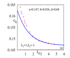
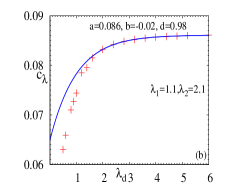
Figure 5: (Color online) Plots (a) and (b) show the variation of $c_{\lambda}$ with $\lambda_{d}$ as shown in Fig. 4 (a) and (d) respectively. Here, it has been seen that both the plots can be fitted with $c_{\lambda}=a+b\exp(-d\lambda_{d})$ for $\lambda_{d}>\lambda_{d}^{u}$ as shown by blue solid lines. It indeed indicates that the effective central charge eventually saturates for strong impurity limit with an exponential damping. The values of fitting parameters are provided inside the plots.

Let us now extensively investigate the behavior of central charge as reflected in $c_{\lambda}$ with $\lambda_{d}$. A clean spin chain (i.e., with $\lambda_{d}=0$) with open boundary condition in one dimension has the central charge $c=1/2$ and $1$ (with $c_{0}=1/12$ and $c_{0}=1/6$) for Ising and anisotropic critical lines respectively. We note that for Figs. 4(b), (c) and (d) with $\lambda_{d}=0$, $c_{0}$ close to $1/12$ which correspond to Ising critical line, whereas for Fig. 4(a), $c_{0}\sim 0.161$ that represents the anisotropic critical line.

For the phase boundaries separating $n=2$ phase from others (see inset of Fig. (4) (a), (c), and (d)), a careful analysis suggests that effective central charge contained in $c_{\lambda}$ that follows the relation: $c_{\lambda}\approx\alpha\log(\lambda_{d})+\beta$ for a range $\lambda_{d}^{l}<\lambda_{d}<\lambda_{d}^{u}$, where the values of $\lambda^{l}_{d}$ and $\lambda^{u}_{d}$ depend on the strengths of $\lambda_{1}$ and $\lambda_{2}$. Afterwards, it eventually saturates with an additional exponential damping term given by $\exp(-\lambda_{d})$ (see Fig. 5). The saturation characteristics of $c_{\lambda}$ for strong impurity limit can be explained by the mathematical form given by $c_{\lambda}=a+b\exp(-d\lambda_{d})$; hence $\lambda_{d}\to\infty$, $c_{\lambda}\to a$.

In contrary, on the $n=1$-$n=0$ phase boundary (with $\lambda_{2}=0$) the effective central charge shows a linear relation with $\lambda_{d}$, $c_{\lambda}=\beta+\alpha\lambda_{d}$. Interestingly, in this case, the value of $\beta$ is close to $c_{0}=1/12$ which is the central charge on that boundary with $\lambda_{d}=0$. Therefore, the term $\alpha\lambda_{d}$ can be considered as the correction over the bare central charge due to the application of the impurity. It is noteworthy that over the complete phase boundary with $\lambda_{2}\neq 0$ and even in the strong impurity limit this linear behavior remains unaffected. Hence it can be inferred that the impurity term indeed plays a distinctly different role in the phase boundaries shared with $n=2$ phase compared to others.

In this connection, we would like to mention that for a disordered quantum spin chain, an effective central charge comes into play instead of the bare central charge obtained in the clean limit refael07 . We here show that even a single impurity term can also lead to an effective central charge. At the same time, this effective central charge has distinct scaling relations with the strength of the impurity over different phase boundaries.

IV.2 Non-equilibrium

In the previous section, we have discussed the influence of the impurity term on both critical and off-critical EE when the system is in equilibrium. Provided the general formalism for calculating the time evolution of the EE with a complex term in the Hamiltonian in Eq. (3) as presented in Sec. III, here we shall now investigate the effect of the impurity term $H_{\rm imp}=-i\lambda_{d}a_{1}a_{2}$ on the evolution of the EE when the Majorana chain is suddenly quenched to various critical points.

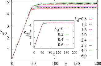
Figure 6: (Color online) Evolution of the EE as a function of time for different values of the impurity strength ($\lambda_{d}$). It can be observed that the EE gets affected by the $\lambda_{d}$ after a certain value of $\lambda_{d}$ when the system is quenched to $n=0$-$n=1$ phase boundary (with $\lambda_{1}=1$ and $\lambda_{2}=0$) from $n=0$ phase with $\lambda_{1}=0.5$. The different curves from bottom to top are given by, solid red line ($\lambda_{d}=0.8$), dashed black line ($\lambda_{d}=1.2$), long-dashed-dotted pink line ($\lambda_{d}=1.6$), double dotted grey line ($\lambda_{d}=2.0$), dashed red line ($\lambda_{d}=2.4$), long-dashed black line ($\lambda_{d}=2.8$), dashed green line ($\lambda_{d}=4.0$), dashed orange line ($\lambda_{d}=6.0$). Inset: It shows that saturation value of the EE is almost independent $\lambda_{d}$ upto some value, say $\lambda_{d}^{*}$. At the same time, main plot depicts that the saturation value of the EE increases logarithmically with $\lambda_{d}$ after $\lambda_{d}^{*}$. Here, block length, $l=20$ and $N=300$.

Let us first assume a situation where $\lambda_{1}$ is suddenly changed from $n=0$ phase to $n=1-n=0$ phase boundary by fixing $\lambda_{2}$ at $0$. The EE after the sudden quench increases linearly up to a time $t^{*}=l/v$ where $v$ is the group velocity of the quasiparticles generated due to the sudden quench (see Fig. 6) and $l$ being the length of subsystem. This phenomena has been explained in the earlier related literature using the picture of quasiparticle propagation through the system after the quench calabrese04 . We find that the group velocity $v$, numerically calculated from the final real space Hamiltonian, is almost independent of $\lambda_{d}$ and it remains at nearly equal to $0.5$ in this case. This also can be observed from Fig. 6 where the EE for a block of length $l=20$ shows a linear rise with time up to $t^{*}\simeq 40$ with different values of $\lambda_{d}$. After time $t=t^{*}$, the EE saturates at some finite values that depend on the strength of $\lambda_{d}$. The inset of Fig. 6 shows that the EE curves almost overlap with each other even in the saturation region up to a threshold value of $\lambda_{d}$, denoted by $\lambda_{d}^{*}$. At the same time, for $\lambda_{d}>\lambda_{d}^{*}$, the saturation value increases with $\lambda_{d}$. It has been observed from the plot that the value of $\lambda_{d}^{*}$ depends only on the final values of parameters $\lambda_{1}$ and $\lambda_{2}$.

One can see from Fig. 7 that the linear behavior of the EE persists up to $t=l$ for the $n=0-n=2$ boundary as $v$ becomes unity there. In contrast to the previous case, here the saturation value of the EE indeed decreases by a small amount with increasing $\lambda_{d}$ when $\lambda_{d}<\lambda_{d}^{*}$. Here also the saturation value of the EE increases with $\lambda_{d}$ after $\lambda_{d}>\lambda_{d}^{*}$. On the other hand, the EE increases linearly up to $t=2l/3$ as $v\simeq 3/2$ over the $n=2-n=1$ phase boundary (see the Fig. (8)). In this case, the decrease of the saturation value of the EE with increasing $\lambda_{d}$ (up to $\lambda_{d}^{*}$) is more prominent than the $n=0-n=2$ boundary. However, the behavior of the EE for $\lambda_{d}>\lambda_{d}^{*}$ seems to be similar to the previous cases.

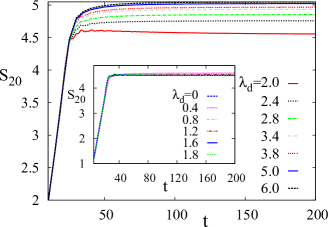
Figure 7: (Color online) Variation of the EE with time after quenching the system to $n=0$-$n=2$ boundary ($\lambda_{1}=1$ and $\lambda_{2}=-1$) from $n=0$ phase with $\lambda_{2}=-0.5$ and $\lambda_{1}=1$. The various curves from bottom to top are given as solid red line ($\lambda_{d}=2.0$), dashed black line ($\lambda_{d}=2.4$), long-dashed-dotted green line ($\lambda_{d}=2.8$), double dotted grey line ($\lambda_{d}=3.4$), dashed red line ($\lambda_{d}=3.8$), solid blue line ($\lambda_{d}=5.0$), long-dashed black line ($\lambda_{d}=6.0$). Here, block length, $l=20$ and $N=300$. Inset plot shows that saturation value of the EE is weakly dependent on $\lambda_{d}$ and decreases by a small amount with increasing the value of $\lambda_{d}$ upto a certain value, say $\lambda_{d}^{*}$. On the other hand, the main plot depicts that the saturation value of EE increases with $\lambda_{d}$ in a non-linear fashion after $\lambda_{d}^{*}$.

We are now interested to determine the relation between the saturation value of the EE and $\lambda_{d}$. It can be observed from Fig. 9 that the variation of the saturation value of EE with $\lambda_{d}$ ($>\lambda_{d}^{*}$) is given by $S_{\rm sat}\propto\log\lambda_{d}$ for all three cases discussed above. The logarithmic behavior of EE suggests the fact that $\lambda_{d}$ affects the EE in an identical manner irrespective of the nature of the phase boundary i.e., whether the phase boundary separates a topological phase from a non-topological phase or two different topological phases. The semiclassical theory of the EE rieger11 suggests that the more number of quasiparticles is generated as one increases the strength of impurity and as a result saturation value of the EE increases with $\lambda_{d}$. However, the logarithmic dependence of saturation value of EE for $\lambda_{d}>\lambda_{d}^{*}$ can not be explained by this theory of quasiparticle generation.

Similar to the variation of $c_{\lambda}$ on the phase boundary shared with $n=2$ phase as shown in Fig. (5), we find that the saturation value of EE eventually approaches to a fixed value with $\lambda_{d}$ for strong impurity limit (see Fig. 10 (a)). In contrary to the equilibrium case, the saturation in $S_{\rm sat}$ is also observed for $n=1$-$n=0$ boundary (see Fig. 10 (b)), whereas $c_{\lambda}$ shows linear variation for whole range of $\lambda_{d}$ there. The strong impurity limit here is meant to be above the range of $\lambda_{d}$ within which logarithmic rise of $S_{\rm sat}$ is observed. As described earlier, it might be the case that after a cut-off value of $\lambda_{d}$ the rate of quasiparticle generation decreases with an exponential damping factor resulting $S_{\rm sat}=a+b\exp(-\lambda_{d})$ for strong impurity limit. It can be noted that the ranges of $\lambda_{d}$ within which the logarithmic rise in $c_{\lambda}$ and $S_{\rm sat}$ occurs following saturation are different from each other.

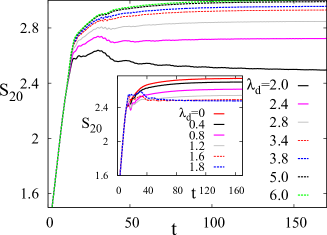
Figure 8: (Color online) Time-evolution of the EE is affected by the impurity strength as the system is quenched to $n=1$-$n=2$ boundary (with $\lambda_{1}=1$ and $\lambda_{2}=2$) from $n=2$ phase with $\lambda_{1}=0.5$ and $\lambda_{2}=2$. The different curves from bottom to top are denoted by solid black line ($\lambda_{d}=2.0$), solid pink line ($\lambda_{d}=2.4$), solid grey line ($\lambda_{d}=2.8$), long-dashed red line ($\lambda_{d}=3.4$), long-dashed blue line ($\lambda_{d}=3.8$), long-dashed black line ($\lambda_{d}=5.0$), long-dashed green line ($\lambda_{d}=6.0$). Here, block length, $l=20$ and $N=300$. Inset: It can be seen that the saturation value of the EE decreases slowly when $\lambda_{d}$ increases up to a certain value $\lambda_{d}^{*}$. Main plot: Similar to the previous cases, after $\lambda_{d}^{*}$, the saturation value of the EE increases with $\lambda_{d}$ in a non-linear fashion.

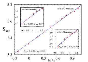
Figure 9: (Color online) We have plotted the saturation value of the EE as a function of $\ln\lambda_{d}$ for three different cases studied in Figs. 6, 7 and 8. This plot shows that saturation value of the EE increases linearly with $\ln\lambda_{d}$ after $\lambda_{d}^{*}$. The blue dashed lines represent the fitted curve: $S_{\rm sat}=\alpha\ln\lambda_{d}+\beta$.

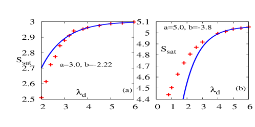
Figure 10: (Color online) Variation of $S_{\rm sat}$ as a function of $\lambda_{d}$ when the quenching is performed up to (a) $n=1$-$n=2$ and (b) $n=1$-$n=0$ phase boundaries. After a logarithmic increase, $S_{\rm sat}$ follows the relation $c_{\lambda}=a+b\exp(-\lambda_{d})$ (depicted by blue solid lines).

For a global quench to a critical point it has been shown that the EE follows the relations $S_{l}\sim c~{}t$ for $t<l/v$ and $S_{l}\sim c~{}l$ for $t>l/v$ calabrese05 ; therefore, the central charge plays a crucial role in both the temporal regions. In our case, interestingly, the linear rise of EE with $t$ remains almost unaltered even if $c_{\lambda}$ (i.e., essentially the effective central charge) depends on $\lambda_{d}$, although, some minor changes occur in a small time window where the linear rise terminates and the saturation starts. On the other hand, saturation values of EE behave in an identical manner as exhibited by $c_{\lambda}$ for boundaries shared with $n=2$ phase. Therefore, the upshot of $\lambda_{d}$ on the effective central charge gets imprinted on the saturation characteristics of EE. Considering the complete non-equilibrium evolution over all the phase boundaries, one can say that the outcome of the effective central charge seems to behave differently with $\lambda_{d}$ as compared to the static limit.

In the present context, one can easily note the difference between equilibrium and non-equilibrium scenarios. The non-equilibrium case which we consider can be illustrated as two simultaneous quenches comprising of a global and a local quench. The global quench is performed by changing a parameter of the Hamiltonian up to a critical point, whereas addition of an impurity term at one end of the chain can be considered as a local quench. Therefore the behaviour of the EE with time is determined by both the quenches unlike the situation to the equilibrium case where one impurity term is added in the critical chain. This might be one of the reasons why the linear rise of the EE with time is not noticeably affected by the impurity term. In other words, for linear rise of the EE global quench dominates and effectively central charge remains unaffected by the impurity term. In addition, this anomalous behavior may be due to the fact that the EE in static limit is governed by low energy properties of the ground state only, whereas, due to the sudden quench, the behavior of EE in non-equilibrium case is substantially determined by the excited energy levels. In this connection, we would like to mention that the contribution from higher excited state is extensively studied using the spectral function following a sudden quench between two different phases in the Lipkin-Meshkov-Glick model campbell16 .

V Conclusions

We investigate the critical characteristics of EE in both equilibrium and non-equilibrium situations by considering the effect of the impurity in a three spin interacting model. We show that the topological phase transitions can be detected by the derivative of EE that shows cusps in the vicinity of the phase boundaries. By applying the impurity term we can probe that the edge modes do contribute in the EE. Additionally, our study suggests that the equilibrium EE satisfies a finite size scaling relation $l^{-1}\ln l$. Interestingly, similar to disordered systems, the application of a single impurity in the system leads to the effective central charge while keeping the critical scaling relation (i.e., $\log l$) of the EE unchanged. For phase boundaries connected with $n=2$ phase, we find that the effective central charge shows a logarithmic scaling relation with $\lambda_{d}$ in a certain range of $\lambda_{d}$ following the saturation with an exponentially damping factor at large $\lambda_{d}$. At the same time, the central charge acquires a linear correction as a function of $\lambda_{d}$ over the bare value at the phase boundary separating $n=0$ and $n=1$ phases.

Furthermore, we extend our study to the time-evolution of the EE following the a critical quench where the impurity term is only added to the boundary of the quenched critical chain. In this case, we focus on the effect of the impurity Hamiltonian on the saturation value of the EE as the linear rise remains unaffected. Our study indicates that irrespective of the phase boundaries there exists a threshold value of the impurity strength after which the saturation value of the EE increases logarithmically with impurity strength. The threshold value of the impurity depends on the final parameters of the critical Hamiltonian. In the strong impurity limit, the increase of saturation value of EE with $\lambda_{d}$ is suppressed by an exponential damping factor.

It has been observed that the effect of the impurity term shows up differently in the EE under equilibrium and non-equilibrium situations i.e., change in the effective central charge due to impurity, as probed in the equilibrium analysis of EE, is substantially visible in the later temporal saturation of EE not in the initial rise with time. We provide two probable reasons for this anomalous behavior. One is related to the competitive effects of two simultaneous quenches. The another one is due to the fact that the higher excited energy levels contribute in the dynamics of EE, whereas, equilibrium behavior of EE is completely governed by the ground state. However, in both the equilibrium and non-equilibrium cases, the range of $\lambda_{d}$ within which the effects are appreciably visible depends on the phase boundary and the values of the other parameters.

In recent years entanglement entropy serves as an indicator of thermalization and many body localization. We would like to mention a few commnents in that direction. General belief says that the ballistic growth (i.e, linear in time) of EE is a signature of thermalization for non-integrable systems kim13 . Although, in our case the impurity term, being quadratic in fermionic operator, is not able to break the integrability of the system, we find a linear rise of EE followed by a saturation. On the other hand, logarithmic growth of EE for many body localized state is clearly distinguished from the dynamical evolution of EE in thermalized phase nanduri14 .

Appendix A Entanglement entropy

To calculate the EE in Eq. (1), we first have to determine the reduced density matrix $\rho_{l}$. The non-local nature of the underlying Jordan-Wigner fermion allows us to construct a $2l\times 2l$ correlation matrix, given by

$$\biggr{[}\Gamma^{A}_{l}\biggl{]}_{2l\times 2l}=\biggl{[}W^{\dagger}\biggr{]}_{2l\times 2N}\biggl{[}\Gamma^{B}\biggr{]}_{2N\times 2N}\biggl{[}W\biggr{]}_{2N\times 2l}.$$ (15)

The matrix $\Gamma^{A}_{l}$ is a skew-symmetric matrix which can be represented into the block-diagonal form $\Gamma^{C}_{l}=V\Gamma^{A}_{l}V^{\dagger}$ by an orthogonal transformation with $V$. Then the matrix $\Gamma^{C}_{l}$ can be written as

$$\Gamma^{C}_{l}=\bigoplus_{j=1}^{l}\left[\begin{array}[]{cc}0&\eta_{j}\\ -\eta_{j}&0\end{array}\right].$$ (16)

This defines a new set of Majorana fermion operators

$$c_{p}=\sum_{q=1}^{2l}V_{pq}e_{q}.$$ (17)

In this basis, the new correlation matrix is given by

$$\langle c_{p}c_{q}\rangle=\delta_{pq}+i(\Gamma^{C}_{l})_{pq}.$$ (18)

The Eq. (16) indicates that the $c$ Majorana fermions are correlated when their site indices are separated by $1$. We use this fact in our next steps of calculations.

Finally, we express the Majorana fermions in terms of usual complex fermions. We define $l$ fermionic modes from $2l$ Majorana operators

$$f_{j}=\frac{c_{2j-1}+ic_{2j}}{2}.$$ (19)

By definition the fermionic modes satisfy the relations

$$\langle f_{j}f_{k}\rangle=0,\hskip 5.69054pt\langle f_{j}^{\dagger}f_{k}\rangle=\delta_{jk}\frac{1+\eta_{j}}{2}.$$ (20)

It signifies that there has no correlation among the $l$ fermionic modes. Using this fact the density matrix of the $l$ fermionic modes can be written as a direct product of $l$ uncorrelated modes $\rho_{l}=\otimes_{n=1}^{l}\varrho_{n}$ with each $\varrho_{n}$ having eigenvalues $(1\pm\eta_{n})/2$. Now, from definition of the EE in Eq. (1), it is given by

$$S(l)=-\sum_{n=1}^{l}\big{[}\big{(}{1+\eta_{n}\over 2}\big{)}\log\big{(}{1+\eta_{n}\over 2}\big{)}+\big{(}{1-\eta_{n}\over 2}\big{)}\log\big{(}{1-\eta_{n}\over 2}\big{)}\big{]}.$$ (21)

References

- (1)
- (2) S-J Gu, Int. J. Mod. Phys. B 24, 4371 (2010).
- (3) H. T. Quan, Z. Song, X. F. Liu, P. Zanardi, and C. P. Sun, Phys. Rev. Lett. 96, 140604 (2006).
- (4) B. Damski, H. T. Quan, W. H. Zurek, Phys. Rev. A 83, 062104 (2011).
- (5) W. K. Wootters, Qunatum Inf. Comput. I, 27 (2001), M. Horodecki, Qunatum Inf. Comput. I, 3 (2001).
- (6) A. Osterloh, L. Amico, G. Falci and R. Fazio, Nature 416, 608 (2002), T. J. Osborne and M. A. Nielsen, Phys. Revs. A, 66, 032110 (2002).
- (7) H. Ollivier and W. H. Zurek, Phys. Rev. Lett. 88, 017901 (2001); W. H. Zurek, Rev. Mod. Phys. 75, 715 (2003).
- (8) G. Vidal, J. I. Latorre, E. Rico, and A. Kitaev, Phys. Rev. Lett. 90, 227902 (2003).
- (9) A. Kitaev and C. Laumann, arXiv:0904.2771v1 (2009), J. C. Budich, S. Walter and B. Tranzettel, Phys. Rev. B 85, 121405 (R) 2012, M. J. Scmidt, D. Rainis and D. Loss, Phys. Rev. B 86, 085414 (2012), S. Tewari, S. D. Sarma, C. Nayak, C. Zhang, and P. Zoller, Phys. Rev. Lett. 98, 010506 (2007).
- (10) T. Nag, U. Divakaran and A. dutta, Phys. Rev. B, 86 020401 (R) (2012).
- (11) R. Sachdeva, T. Nag, A. Agarwal, and A. Dutta, Phys. Rev. B 90, 045421 (2014)
- (12) S. Suzuki, T. Nag and A. Dutta, Phys. Rev. A, 93, 012112(2016).
- (13) T. Nag, Phys. Rev. E 93 062119 (2016).
- (14) T. Nag, and A. Dutta, Phys. Rev. A 94, 022316 (2016).
- (15) A. Rajak, and U. Divakaran, JSTAT 043107 (2016).
- (16) B. K. Chakrabarti, A. Dutta and P. Sen, Quantum Ising Phases and transitions in transverse Ising Models, m41 (Springer, Heidelberg,1996).
- (17) S. Sachdev, Quantum Phase Transitions(Cambridge University Press, Cambridge, England,1999).
- (18) A. Polkovnikov, K. Sengupta, A. Silva and M. Vengalattore, Rev. of Mod. Phys. 83, 863 (2011).
- (19) A. Dutta, G. Aeppli, B. K. Chakrabarti, U. Divakaran, T. Rosenbaum and D. Sen, Quantum Phase Transitions in Transverse Field Spin Models: From Statistical Physics to Quantum Information (Cambridge University Press, Cambridge, 2015).
- (20) P. Calabrese and J. Cardy, J. Stat. Mech. P06002 (2004).
- (21) G. Refael and J. E. Moore, Phys. Rev. B 76, 024419 (2007).
- (22) I. Peschel, J. Phys. A: Math. Gen. 38, 4327–4335 (2005).
- (23) H. Li and F. D. M. Haldane, Phys. Rev. Lett. 101, 010504 (2008).
- (24) H. Yao and X-L Qi, Phys. Rev. Lett. 105, 080501 (2010).
- (25) L. Fidkowski, Phys. Rev. Lett. 104, 130502 (2010).
- (26) F. Pollmann, A. M. Turner, E. Berg, and M. Oshikawa, Phys. Rev. B 81, 064439 (2010).
- (27) P. Facchi, U. Marzolino, G. Parisi, S. Pascazio, and A. Scardicchio, Phys. Rev. Lett. 101, 050502 (2008).
- (28) M. Z. Hasan and C.L. Kane, Rev. Mod. Phys. 82, 3045 (2010).
- (29) X.-L. Qi and S.-C. Zhang, Rev. Mod. Phys. 83, 1057 (2011).
- (30) S. Ryu and Y. Hatsugai, Phys. Rev. B 73, 245115 (2006).
- (31) A. Kitaev and J. Preskill, Phys. Rev. Lett. 96, 110404 (2006), M. Levin and X.G. Wen, Phys. Rev. Lett. 96, 110405 (2006).
- (32) J. Borchmann, A. Farrell, S. Matsuura, and T. Pereg- Barnea, Phys. Rev. B 90, 235150 (2014), T. P. Oliveira, P. Ribeiro, P. D. Sacramento, J. Phys.: Condens. Matter 26 425702 (2014), J. Borchmann, A. Farrell, T. P-Barnea, Phys. Rev. B 93, 125133 (2016).
- (33) P. Calabrese and J. Cardy, J. Stat. Mech., P04010 (2005).
- (34) V. Eisler and I. Peschel, J. Stat. Mech., P06005 (2007).
- (35) P. Calabrese and J. Cardy, J. Stat. Mech., P10004 (2007).
- (36) V. Eisler, D. Karevski, T. Platini, and I. Peschel, J. Stat. Mech., P01023 (2008).
- (37) F. Igloi, Z. Szatmari, and Y. -C. Lin, Phys. Rev. B 80, 024405 (2009).
- (38) B. Hsu, E. Grosfeld, and E. Fradkin, Phys. Rev. B 80, 235412 (2009).
- (39) J. Cardy, Phys. Rev. Lett. 106, 150404 (2011).
- (40) I Bloch, J. dalibard, and W. Zwerger, Rev. Mod. Phys. 80, 885 (2008).
- (41) T. Kinoshita, T. Wenger, and D. S. Weiss, Phys. Rev. Lett. 95, 190406 (2005).
- (42) T. Kinoshita, T. Wenger, and D. S. Weiss, Nature 440, 900 (2006).
- (43) F. Igloi, Z. Szatmari, and Y. -C. Lin, Phys. Rev. B 85, 094417 (2012).
- (44) M.-C. Chung, Y. -H. Jhu, P. Chen, C.-Y. Mou, and X. Wan, arXiv:1401.0433.
- (45) M. Cheneau etal., Nature 481, 484–487 ( 2012).
- (46) R. Islam etal., Nature 528, 77–83 ( 2015).
- (47) A. Kitaev, Physics-Uspekhi 44, 131 (2001),arXiv:cond-mat/0010440v2 (2000).
- (48) I. C. Fulga, F. Hassler, A. R. Akhmerov, and C. W. J. Beenakker, Phys. Rev. B 83, 155429 (2011).
- (49) J. D. Sau and S. Das Sarma, Nature communications 3, 964 (2012).
- (50) R. M. Lutchyn and M. P. A. Fisher, Phys. Rev. B 84, 214528 (2011).
- (51) W. DeGottardi, D. Sen, and S. Vishveshwara, New J. Phys. 13, 065028 (2011).
- (52) W. DeGottardi, D. Sen, and S. Vishveshwara, Phys. Rev. Lett. 110, 146404 (2013).
- (53) M. Thakurathi, A.A. Patel, D. Sen, and A. Dutta, Phys. Rev. B 88, 155133 (2013).
- (54) W. DeGottardi, M. Thakurathi, S. Vishveshwara, and D. Sen, Phys. Rev. B 88 165111 (2013).
- (55) J. Alicea, Rep. Prog. Phys. 75, 076501 (2012).
- (56) A. Rajak and A. Dutta, Phys. Rev. E 89, 042125 (2014).
- (57) A. Rajak, T. Nag and A. Dutta, Phys. Rev. E 90, 042107 (2014).
- (58) A. Kopp and S. Chakravarty, Nat. Phys., 1, 53 (2005).
- (59) Y. Niu, S. K. Chung, C-H Hsu, I. Mandal, S. Raghu and S. Chakravarty, Phys. Rev. B 85, 035110 (2012).
- (60) A. Rajak and T. Nag, Phys. Rev. E 96, 022136 (2017).
- (61) W. Son, L. Amico, R. Fazio, A. Hamma, S. Pascazio, and V. Vedral, Europhys. Lett. 95, 50001 (2011).
- (62) S M Giampaolo and B C Hiesmayr, New J. Phys. 16, 093033 (2014).
- (63) B. -e. Friedman, A. Rajak, A. Russomanno, and E. G. D. Torre, arXiv:1708.03400v2 (2017).
- (64) T. J. G. Apollaro, G. Francica, D. Giuliano, G. Falcone, G. M. Palma, and F. Plastina, Phys. Rev. B 96, 155145 (2017).
- (65) X. Huang, and, Z. Yang, Solid State communications, 204, 28-32 (2015).
- (66) T. Fukuhara et al., Nat. Phys. 9, 235 (2013).
- (67) J. I. Latorre, E. Rico, and G. Vidal, Quant. Inf. Comput. 4, 48-92 (2004).
- (68) S. J. Gu, Int. J. Mod. Phys. B 24, 4371 (2010).
- (69) S. Sharma and A. Rajak, J. Stat. Mech., P08005 (2012).
- (70) A. Rajak and U. Divakaran, J. Stat. Mech., P04023 (2014).
- (71) M. S. Sarandy, Phys. Rev. A 80, 022108 (2009).
- (72) R. Dillenschneider, Phys. Rev. B 78, 224413 (2008).
- (73) Y. Wang, T. Gulden, and A. Kamenev, Phys. rev. B, 95, 075401 (2017).
- (74) T. Gulden, M. Janas, Y. Wang, and A. Kamenev, Phys. Rev. Lett. 116, 026402 (2016).
- (75) H. Rieger, Ferenc Igloi, Phys. rev. B, 84, 165117 (2011).
- (76) S. Campbell, Phys. Rev. B 94, 184403 (2016).
- (77) H. Kim, and D. A. Huse, Phys. Rev. Lett. 111, 127205 (2013).
- (78) A. Nanduri, H. Kim, and D. A. Huse, Phys. Rev. B 90, 064201 (2014).