Functionality of Disorder in Muscle Mechanics

Abstract

A salient feature of skeletal muscles is their ability to take up an applied slack in a microsecond timescale. Behind this remarkably fast adaptation is a collective folding in a bundle of elastically interacting bistable elements. Since this interaction has long-range character, the behavior of the system in force and length controlled ensembles is different; in particular, it can have two distinct order-disorder–type critical points. We show that the account of the disregistry between myosin and actin filaments places the elementary force-producing units of skeletal muscles close to both such critical points. The ensuing "double-criticality" contributes to the system’s ability to perform robustly and suggests that the disregistry is functional.

If an isometrically activated muscle is suddenly shortened, the force first abruptly decreases but then partially recovers over $\sim$ 1 ms timescale Podolsky (1960); Huxley and Simmons (1971); Irving et al. (1992). Behind this remarkably swift contraction is a cooperative conformational change in an assembly of actin-bound myosin heads (cross bridges). Given that this "power stroke" takes place at a timescale that is much shorter than the timescale of the adenosine triphosphate (ATP)-driven attachment-detachment ($\sim$ 100 ms) Howard (2001); Piazzesi et al. (2002); Kaya et al. (2017), such fast force recovery is usually interpreted as a passive phenomenon Vilfan and Duke (2003); Marcucci and Truskinovsky (2010).

If it is an applied force, which is controlled, the mean-field theory of fast force recovery, viewing filaments as rigid and cross bridges as parallel Caruel and Truskinovsky (2016), predicts metastability associated with a coherent response Caruel et al. (2013). It also predicts the existence of an order-disorder–type critical point, and it was argued that this critical point plays an essential role in the functioning of the muscle machinery Caruel and Truskinovsky (2017, 2018). This is consistent with the fact that critical systems are ubiquitous in biology because of their adaptive advantages, in particular, their robustness in the face of random perturbations Balleza et al. (2008); Beggs and Timme (2012); Mora and Bialek (2011); Krotov et al. (2014); Kessler and Levine (2015). Criticality is often linked to marginal stability and, indeed, skeletal muscles are known to exhibit near zero passive rigidity in physiological (isometric contractions) conditions Huxley and Simmons (1971); Brunello et al. (2014); Piazzesi et al. (2007); Linari et al. (1998).

The mechanical functioning of this force generated system system is complicated by the fact that muscle architecture involves both parallel and series connections (see Fig. 1). Parallel elements respond to a common displacement (hard device, Helmholtz ensemble), while series structures sense a common force (soft device, Gibbs ensemble). To fold coherently, individual contractile units should be able to coordinate in both types of loading conditions; however, the dominance of long-range interactions Campa et al. (2009); Barré et al. (2001) induces different collective behavior in force and length controlled ensembles Caruel et al. (2013). In particular, the critical points corresponding to length and force clamp loading conditions are strictly distinct Caruel and Truskinovsky (2018).

In realistic conditions, however, they turn out to be close to each other and, to ensure the robustness of the response under a broad range of mechanical stimuli (flexibility) Muñoz (2018), the system can still be poised in the vicinity of both critical points.

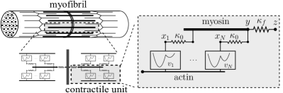
Figure 1: Schematic representation of a muscle myofibril, of an elementary contractile unit (half-sarcomere) and of a parallel bundle of $N$ cross bridges. In the model, the double-well potentials are mimicked by spin variables.

In this Letter, we argue that such "double criticality" is actualized in the system of muscle cross bridges due to quenched disorder. While skeletal muscles are often compared to ideal crystals, the perfect ordering is compromised by the intrinsic disregistry between the periodicities of myosin cross bridges and actin binding sites. Binding of cross bridges is restricted to incompatibly placed segments on actin filaments (target zones), and experimental studies based on electron microscopy and x-ray diffraction suggest that myosin heads are bound to actin at seemingly random positions Tregear et al. (1998, 2004). To gain an insight into the role of variable offsets, we assume that the attachment sites are indeed chosen at random and show that this gives us an analytically tractable model.

The idea that actomyosin disregistry brings the system’s stiffness to zero was pioneered in Huxley and Tideswell (1996). More recently the utility of quenched disorder for the active aspects of muscle mechanics has been advocated in Egan et al. (2017). The beneficial role of random inhomogeneity has been established in many other fields of physics from high-temperature superconductivity in electronic materials Zaanen (2010) to Griffiths phases in brain networks Moretti and Muñoz (2013).

To explore the reachability of the "double criticality" condition in realistic conditions, we reduce the description of the system of interacting cross bridges to a random field Ising model (RFIM) and compute the equilibrium free energy applying techniques from the theory of glassy systems Castellani and Cavagna (2005). We then use the available experimental data on skeletal muscles to justify the claim that quenched disorder is the main factor ensuring the targeted mechanical response.

We associate with each cross bridge a spin variable $x$ taking the value $0$ in the pre-power-stroke state (unfolded conformation) and $-1$ in the post-power-stroke state (folded conformation). Each spin element is then placed in series with a linear elastic spring of stiffness $\kappa_{0}$. If we nondimensionalize lengths by the power-stroke size $a$ and energy by $\kappa_{0}a^{2}$, the dimensionless energy of a cross bridge reads $(1+x)v+\frac{1}{2}(y-x)^{2},$ where $y$ is the dimensionless displacement of myosin relative to actin and $v$ is the dimensionless energetic bias, see Fig.1. To model disregistry, we assume that the parameter $v$ is different for different cross bridges .

Consider now a parallel bundle of $N$ cross bridges shown schematically in Fig. 1. Individual cross bridges are attached to a backbone composed of myosin tails. The elasticity of the backbone can be accounted through a lump spring of stiffness $\kappa_{f}$ in series with the bundle Linari et al. ; Caruel et al. (2015); Jülicher and Prost (1995). The system loaded in a hard device is then characterized by the dimensionless energy

$$E=\sum_{i=1}^{N}[(1+x_{i})v_{i}+\frac{1}{2}(y-x_{i})^{2}]+N\frac{\lambda_{f}}{2}(z-y)^{2},$$ (1)

where $z$ is the applied displacement and $\lambda_{f}=\kappa_{f}/(N\kappa_{0})$. We assume that the parameters $v_{i}$ are independent identically distributed random variables with probability density $p(v)$.

If we replace variables $x_{i}$ by $s_{i}=2x_{i}+1=\pm 1$ and adiabatically eliminate $y$, assuming that $\partial E/\partial y=0$, the energy (1) takes the form

$$E=-J/(2N)\sum_{i,j}s_{i}s_{j}-\sum_{i}h_{i}s_{i}+c,$$

where $J=1/4(1+\lambda_{f})$, $c$ is a $z$ dependent constant, and the coefficients $h_{i}$ are linear in $v_{i}$ (see Supplemental Material SM ). We can then conclude that (1) is a version of the mean-field RFIM, which is explicitly solvable Schneider and Pytte (1977); Krzakala et al. (2010).

Using the self-averaging property of the free energy in the thermodynamic limit, we write

$$\mathcal{F}(\beta,z)=-\lim_{N\rightarrow\infty}(N\beta)^{-1}\langle\log\mathcal{Z}(\beta,z;\{v\})\rangle_{v},$$

where the averaging $\langle\cdot\rangle_{v}$ is over the disorder, $\beta=\kappa_{0}a^{2}/(k_{B}T)$, and

$$\mathcal{Z}=\displaystyle\int dy\sum_{x\in\{0,-1\}^{N}}\exp(-\beta E(\bm{x},y,z;\{v\}).$$

In the thermodynamic limit, we obtain SM

$$\begin{split}\mathcal{F}(\beta,z)&=\frac{\lambda_{f}}{2}(z-y_{0})^{2}+\frac{1}{4}(y_{0}+1)^{2}+\frac{1}{2}(\frac{y_{0}^{2}}{2}+v_{0})\\ &-\frac{1}{\beta}\int dv\,p(v)\log\left[2\cosh[\frac{\beta}{4}(1+2y_{0}-2v)]\right],\end{split}$$ (2)

where $y_{0}$ must solve the self-consistency equation

$$y_{0}=\frac{2\lambda_{f}z-1}{2(\lambda_{f}+1)}+\int dv\,\frac{p(v)}{2(\lambda_{f}+1)}\tanh\left[\frac{\beta}{4}(1-2v+2y_{0})\right].$$ (3)

The multiplicity of solutions of Eq. (3) is a result of the nonconvexity of the free energy with respect to $y$, which is ultimately an effect of long-range interactions. The multiplicity leads to the possibility of discontinuous tension-elongation curves $t=\partial\mathcal{F}/\partial z=\lambda_{f}(z-y_{0})$.

If we assume that the disorder is Gaussian $p(v)=(2\pi\sigma^{2})^{-1/2}\exp(-\frac{(v-v_{0})^{2}}{2\sigma^{2}})$, the behavior of the system will be fully defined by the temperature $1/\beta$, the variance of disorder $\sigma^{2}$, and the parameter $\lambda_{f}$, characterizing the degree of elastic coupling. The resulting phase diagram is shown in Fig. 2. The disorder-free section $\sigma=0$ of this diagram was previously studied in Caruel and Truskinovsky (2018). At $\sigma>0$ the system responds as if it was subjected to a higher effective temperature Roux (2000); Politi et al. (2002). The Helmholtz free energy $\mathcal{F}(\beta,z)$ and the tension-elongation relations $t(\beta,z)$ in the three phases I, II, and III are illustrated in Fig. 3.

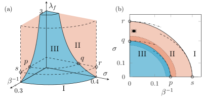
Figure 2: (a) Configuration of phases I, II, and III in the parameter space ($1/\beta$, $\sigma$ , $\lambda_{f}$). (b) A section of this phase diagram corresponding to $\lambda_{f}=0.54\pm 0.2$; the shadowed region near the boundary of II and III reflects the uncertainty in $\lambda_{f}$. The realistic dataset for skeletal muscles is presented in (b) by a filled circle with the superimposed error bars indicating uncertainty in temperature. Analytic approximations in (b): dashed-dotted lines indicate low temperature; dashed lines indicate low disorder.

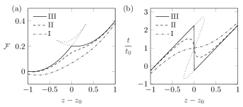
Figure 3: (a) Representative Helmholtz free energies in each of the phases I, II, III. (b) The corresponding tension-elongation relations; $z_{0}=(1+\lambda_{f})v_{0}/\lambda_{f}-1/2$; $t_{0}=v_{0}$.

In phase I, the cooperativity is absent and the cross bridges fluctuate independently. In phase III, the cross bridges can synchronously switch between two "pure states". In the intermediate phase II, the tension-elongation relation exhibits negative stiffness. The boundary between phases II and III is defined by the condition that $\partial^{2}\tilde{\mathcal{F}}(\beta,z,y)/\partial y^{2}=0$, which is a condition that the three roots of (3) collapse into one.

In the limiting case $\sigma\rightarrow 0$, the point $p$ in Fig. 2(b) is at $\beta=4(\lambda_{f}+1)$. Around this point, the $p-q$ curve is described accurately by the low-disorder approximation $\beta_{e}=4(\lambda_{f}+1)$ where $\beta_{e}=(\beta^{-2}+\sigma^{2}/2)^{-1/2}$ is the inverse effective temperature (see Supplemental Material SM ). In another limiting case $\beta\rightarrow\infty$, the point $q$ can be found from the equation $\sigma=1/\sqrt{2\pi(\lambda_{f}+1)}$ and around this point the $p-q$ curve is given by the small temperature approximation $\sigma_{e}=1/\sqrt{2\pi(\lambda_{f}+1)}$, where $\sigma_{e}^{2}=(\sigma^{2}+2\beta^{-2})=2\beta_{e}^{-2}$ is the variance of the effective disorder SM .

The boundary between phases II and III marks a second-order phase transition: the order parameter $\phi=N^{-1}\sum_{i=1}^{N}\left<s_{i}\right>_{\beta}$, where $\langle\cdot\rangle_{\beta}$ is the thermal average, is double valued in phase III and single valued in phase II. To distinguish between different microscopic configurations, we also compute the Edwards-Anderson (overlap) parameter $q_{\text{EA}}=N^{-1}\sum_{i=1}^{N}\langle\langle s_{i}\rangle^{2}_{\beta}\rangle_{v}$ SM . If $q_{\text{EA}}\neq 0$ while $\phi=0$, the pre- and post-power-stroke symmetry is broken and cross bridges may be locally frozen in either of the two states, even though such local ordering in time does not imply any spatial order. Figure 4 shows that $q_{\text{EA}}$ is indeed different from zero in the phase II close to the $p-q$ boundary, which indicates weakly glassy behavior Schneider and Pytte (1977); Vilfan (1987); Krzakala et al. (2010). This is a hint that, in a more realistic model, where the finite backbone stiffness is taken into account, a real "strain glass" phase Wang et al. (2006); Vasseur et al. (2012) is likely to appear.

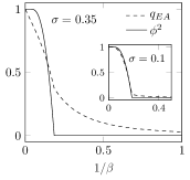
Figure 4: The behavior of the parameter $\phi^{2}$ (solid lines) and the Edwards-Anderson parameter $q_{\text{EA}}$ (dashed lines) near the boundary between phases II and III at the realistic value of disorder. (Inset) The case of weak disorder.

To find the boundary between phases I and II, we need to solve the equation $\partial^{2}\mathcal{F}/\partial z^{2}=0$ or $\partial y_{0}/\partial z=1$, where $y_{0}$ is a solution of (3). When $\sigma=0$, we obtain $\beta=4$, which defines the location of point $s$ in Fig. 2(b) (see also Caruel et al. (2013, 2015)). The low-disorder approximation gives $\beta_{e}=4$. In another limiting case $\beta\rightarrow\infty$, the location of the point $r$ in Fig. 2(b) is given by $\sigma=\sigma_{e}=\sqrt{1/2\pi}$.

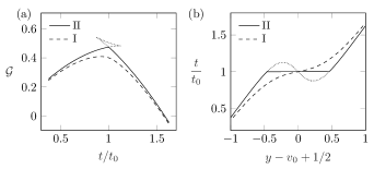
Figure 5: (a) Representative Gibbs free energies in each of the phases I and II. (b) The corresponding tension-elongation curves; $z_{0}=(1+\lambda_{f})v_{0}/\lambda_{f}-1/2$; $t_{0}=v_{0}$.

The boundary between the phases I and II can be also interpreted as a line of second-order phase transitions, but now in the soft device (force clamp) ensemble. In this case, the presence of a series spring is irrelevant and we can assume that $\lambda_{f}\rightarrow 0$, $z\rightarrow\infty$, but $\lambda_{f}z\rightarrow t$, where tension $t$ is the new control parameter. Following the approach used in the case of a hard device, we similarly obtain the Gibbs free energy $\mathcal{G}(\beta,t)$ and compute the tension-elongation relation $y=-\partial\mathcal{G}/\partial t$, (see Supplemental Material SM ).

In Fig. 5, we show that the soft device tension-elongation relation in phase II is monotone but discontinuous. On the boundary of I and II [see Fig. 2(b)], the stiffness becomes zero in stall conditions, which means that it is a set of critical points in the soft device ensemble. This line, targeted numerically in Huxley and Tideswell (1996), represents regimes that can be expected to deliver the optimal trade-off between robustness and flexibility in the soft device Kauffman (1993); Darabos et al. (2011).

So far, we have operated under an implicit assumption that in the thermodynamic limit $\kappa_{f}\to\infty$, while $\lambda_{f}$ remains finite. This assumption is based on the picture of a myosin filament as a parallel arrangement of $N$ myosin tails, all contributing to the lump stiffness of the backbone. An alternative assumption may be that the effective stiffness of the backbone $\kappa_{f}$ does not depend on the number of attached cross bridges $N$ and, in this case, we have a different scaling $\lambda_{f}\sim N^{-1}$. Then Fig. 2(a), illustrating the size effect, suggests that the quasicritical behavior should be tightly linked to the particular (optimal) number of cross bridges.

To apply our results to a realistic muscle system, we use the data for Rana temporaria at $T=277.15$ K Caruel and Truskinovsky (2018). From structural analysis, we obtain the value $a\sim 10$ nm Dominguez et al. (1998); Rayment et al. (1993a, b). Measurements of the fiber stiffness in rigor mortis, where all the 294 cross bridges per half-sarcomere were attached, produced the estimate $\kappa_{0}=2.7\pm 0.9$ pN/nm Brunello et al. (2014); Piazzesi et al. (2007). The number of attached cross bridges in physiological conditions is $N=106\pm 11$ and experimental measurements at different $N$ converge on the value $\kappa_{f}=154\pm 8$ pN.nm^-1 for the lump filaments stiffness Wakabayashi et al. (1994); Huxley et al. (1994); Piazzesi et al. (2002). This gives $\lambda_{f}=0.54\pm 0.2$. Knowing $\kappa_{0}$ and $a$ we can estimate the nondimensional inverse temperature to be $\beta=71\pm 26$.

Now, for $y>y_{*}$, where $y_{*}=v_{0}-1/2$, the ground state of a single cross bridge is in the pre-power-stroke state, while for $y<y_{*}$ it is in the post-power-stroke state, so $y_{*}$ represents the characteristic offset for an individual cross bridge. Knowing that $y_{*}\sim 4$nm Huxley and Simmons (1971); Huxley and Tideswell (1996), we conclude that $v_{0}\sim 24.3$pN $/(\kappa_{0}a)$. It was experimentally shown in Tregear et al. (2004) that at least 60$\%$ of the cross bridges are axially displaced within half of the spacing between actin monomers, which corresponds to $\sim 2.76$ nm shift from the nearest actin binding site (see also Huxley and Tideswell (1996)). Given the linear relation between $v_{0}$ and $y_{*}$ with the proportionality coefficient equal to one, the variances of these two quantities are the same. If the axial offsets are Gaussian random numbers, we can estimate the standard deviation of the energetic bias $\sigma\sim 3.3$nm$/a$ (see Supplemental Material SM ).

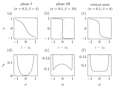
Figure 6: The structure of the energy barriers in different regimes for the case of the hard device. (a)–(c) $z$ dependence of the order parameter $\phi=N^{-1}\sum_{i=1}^{N}\langle s_{i}\rangle$ in different regimes; (d)–(f) matching free energies at fixed $z=z_{0}$. $\lambda_{f}=0.35$ and $v_{0}=0.1$

Based on these data we find that, rather remarkably, the system appears to be operating in a narrow domain of stability of phase II, close to both critical lines $p-q$ and $r-s$ [see the point marked by a filled circle in Fig. 2(b)]. The gap between these boundaries corresponds to $\sim 1$ nm difference in the cross bridge attachment positions, which is rather small given that the size of a single actin monomer is about $5.5$ nm. The mechanical responses in the adjacent critical regimes are structurally similar; however, if in the hard device ensemble we can expect coherent fluctuations of stress (infinite rigidity), in the soft device, criticality would manifest itself through system size correlations of strain (zero rigidity).

The special nature of the critical regimes is illustrated in Fig. 6 for the case of a hard device. In phase I, the response is uncorrelated, and the collective power stroke is impossible [Figs. 6(a) and 6(d)]. In phase III, the response is synchronous but at the cost of crossing an energetic barrier that diverges in the thermodynamic limit ($\mathcal{F}$ is the free energy per cross bridge), which facilitates freezing in the pure states, [see Figs. 6(b) and 6(e)]. The advantage of the critical regime is that the system can perform the collective stroke without crossing a prohibitively high macroscopic barrier, [see Figs. 6(c) and 6(f)]. The analysis is similar for the case of a soft device.

Our study then suggests that evolution might have used quenched disorder to tune the muscle machinery to perform near the conditions where both the Helmholtz and the Gibbs free energies are singular. Such design is highly functional when elementary force-producing units are loaded in a mixed, soft-hard device. We recall that the muscle architecture is characterized by hierarchical structures with coupled modular elements loaded both in parallel and in series. In such systems, the proximity to only one of the two critical points will not be sufficient to ensure high performance in a broad range of conditions Muñoz (2018); Bialek (2018). Moreover, as we show in the Supplemental Material SM , the very idea of ensemble independent local constitutive relations for such systems becomes questionable.

In conclusion, we established new links between muscle physiology and the theory of spin glasses and revealed a tight relation between actomyosin disregistry and the optimal mechanical performance of the force-generating machinery. At a price of neglecting many important features of actual muscles, we were able to focus attention on the role of quenched disorder in the functioning of this biological system. The observed glassiness in the regime of isometric contractions allows the system to access the whole spectrum of rigidities from zero (adaptability, fluidity) to infinite (control, solidity) and may serve as the factor ensuring the largest dynamic repertoire of the "muscle material". Similar disorder-mediated tuning towards criticality can be expected in other biological systems relying on bistability and long-range interactions (Caruel and Truskinovsky, 2016), including hair cells, which employ elastically coupled gating springs Bormuth et al. (2014) and focal adhesions with their cell adhesion molecules bound to a common substrate Schwarz and Safran (2013).

Appendix A Supplemental Material for the paper "Functionality of Disorder in Muscle Mechanics"

A.0.1 Mapping to the Random-Field Ising Model

We start with the energy function (1) in the main text and assume that the internal variable $y$ is eliminated using the condition $\partial E/\partial y=0$. Then,

$$y=\frac{\lambda_{f}z}{1+\lambda_{f}}+\frac{1}{N(1+\lambda_{f})}\sum_{i}x_{i}.$$

and the relaxed energy reads

$$\begin{split}E(x_{i},z)&=-\frac{1}{2N(1+\lambda_{f})}\left(\sum_{i}x_{i}\right)^{2}\\ +\sum_{i}(1&+x_{i})v_{i}-\frac{\lambda_{f}z}{1+\lambda_{f}}\sum_{i}x_{i}+\sum_{i}\frac{x_{i}^{2}}{2}+\frac{N\lambda_{f}z^{2}}{2(1+\lambda_{f})}\end{split}$$

Since $x_{i}$ is either 0 or -1, we may write $\sum_{i}x_{i}^{2}=-\sum_{i}x_{i}$ and $\left(\sum_{i}x_{i}\right)^{2}=\sum_{i}\sum_{j}x_{i}x_{j}=\sum_{i,j}x_{i}x_{j}$. In terms of spin variables, $2x_{i}=s_{i}-1,\,\text{with }s_{i}=\pm 1$ the relaxed energy can be written as,

$$\begin{split}E(s_{i},z)&=-\frac{1}{8N(1+\lambda_{f})}\sum_{i,j}s_{i}s_{j}\\ -&\sum_{i}\left(\frac{2\lambda_{f}z-1}{4(1+\lambda_{f})}+\frac{1}{4}-\frac{v_{i}}{2}\right)s_{i}\\ +&\sum_{i}\left(\frac{\lambda_{f}z(1+z)}{2(1+\lambda_{f})}+\frac{1}{4}+\frac{v_{i}}{2}-\frac{1}{8(1+\lambda_{f})}\right)\\ &=-\frac{J}{2N}\sum_{i,j}s_{i}s_{j}-\sum_{i}h_{i}s_{i}+f(z).\end{split}$$ (4)

where $J=\frac{1}{4(1+\lambda_{f})}$, $h_{i}=\frac{2\lambda_{f}z-1}{4(1+\lambda_{f})}+\frac{1}{4}-\frac{v_{i}}{2}$ and $f(z)=\sum_{i}\frac{\lambda_{f}z(1+z)}{2(1+\lambda_{f})}+\frac{1}{4}+\frac{v_{i}}{2}-\frac{1}{8(1+\lambda_{f})}$.

A.0.2 Computation of the free energy

Using the self-averaging property of the free energy in the thermodynamic limit, we write

$$\mathcal{F}(\beta,z)=-\lim_{N\rightarrow\infty}(N\beta)^{-1}\langle\log\mathcal{Z}(\beta,z;\{v\})\rangle_{v},$$

where the averaging $\langle\cdot\rangle_{v}$ is over the disorder, $\beta=\kappa_{0}a^{2}/(k_{B}T)$, and

$$\mathcal{Z}=\displaystyle\int dy\sum_{x\in\{0,-1\}^{N}}\exp(-\beta E(\bm{x},y,z;\{v\}).$$

The mean field nature of the model allows one to rewrite this expression in the form

$$\mathcal{Z}=\int dy\exp(-\beta N[\frac{\lambda_{f}}{2}(z-y)^{2}-\frac{1}{\beta N}\sum_{i=1}^{N}\log\tilde{\mathcal{Z}}]),$$

where $\tilde{\mathcal{Z}}=e^{-\frac{\beta}{2}(y+1)^{2}}+e^{-\beta(y^{2}/2+v_{i})}$ is the partition function of a single Huxley-Simmons element Huxley and Simmons (1971); Caruel and Truskinovsky (2016). In the thermodynamic limit, we can use the saddle-point approximation to obtain $\mathcal{F}(\beta,z)=\tilde{\mathcal{F}}(y_{0},\beta,z),$ where $\tilde{\mathcal{F}}(y,\beta,z)=\beta\frac{\lambda_{f}}{2}(z-y)^{2}-\langle\log\tilde{\mathcal{Z}}\rangle_{v}$ and $y_{0}(\beta,z)$ is the minimum of $\tilde{\mathcal{F}}$. More explicitly,

$$\begin{split}\mathcal{F}(\beta,z)&=\frac{\lambda_{f}}{2}(z-y_{0})^{2}+\frac{1}{4}(y_{0}+1)^{2}+\frac{1}{2}(\frac{y_{0}^{2}}{2}+v_{0})\\ &-\frac{1}{\beta}\int dv\,p(v)\log\left[2\cosh[\frac{\beta}{4}(1+2y_{0}-2v)]\right],\end{split}$$ (5)

where $y_{0}$ solves the self-consistency equation,

$$y_{0}=\frac{2\lambda_{f}z-1}{2(\lambda_{f}+1)}+\int dv\,\frac{p(v)}{2(\lambda_{f}+1)}\tanh\left[\frac{\beta}{4}(1-2v+2y_{0})\right].$$

A.0.3 Boundary between phases II and III

Using the expression for the partial free energy,

$$\begin{split}\tilde{\mathcal{F}}(\beta,z,y)&=\frac{\lambda_{f}}{2}(z-y)^{2}+\frac{1}{4}(y+1)^{2}+\frac{1}{2}(y^{2}/2+v_{0})\\ &-\frac{1}{\beta}\int dv\,p(v)\log\left[2\cosh[\frac{\beta}{4}(1+2y-2v)]\right]\end{split}$$

we can write the condition $\partial^{2}\tilde{\mathcal{F}}(\beta,z,y)/\partial y^{2}=0$ in the form

$$\lambda_{f}+1-\frac{\beta}{4}\int dv\,p(v)\operatorname{sech}^{2}\frac{\beta}{4}(1-2v+2y_{0})=0.$$

If we use the Gaussian distribution of disorder introduced in the main text and use new variables $\eta=\beta(1+2y_{0})/2$ and $\bar{v}=\beta v$ we can rewrite this equation in the form

$$\lambda_{f}+1-\frac{\beta}{4}\int d\bar{v}\frac{e^{-\frac{(\bar{v}-\beta v_{0})^{2}}{2\sigma^{2}\beta^{2}}}}{\sqrt{2\pi\sigma^{2}\beta^{2}}}\operatorname{sech}^{2}\frac{1}{2}(\eta-\bar{v})=0.$$

Note that the variance of disorder appears in this formula only in the combination $\sigma^{2}\beta^{2}$. This means that, modulo some obvious adjustments, the small disorder $\sigma\to 0$ and large temperature $\beta\to 0$ limits are complimentary. The same can be said about the small temperature $\beta\to\infty$ and the large disorder $\sigma\to\infty$ limits.

Zero disorder limit. In the limit $\sigma\rightarrow 0$ we have $p(v)\rightarrow\delta(v-v_{0})$ and the boundary between phase II and III is defined by the equation

$$\lambda_{f}+1=\frac{\beta}{4}\operatorname{sech}^{2}\frac{\beta}{4}(1-2v_{0}+2y_{0}).$$

Since $\operatorname{sech}^{2}x\in[0,1]$, this equation does not have solutions $y_{0}$ for $\beta>4(\lambda_{f}+1)$ and therefore the point $r$ is defined by the condition $\beta=4(\lambda_{f}+1)$.

To get the next term of the asymptotic expansion we introduce the new variable $\xi=(1-2v+2y_{0})/4$ and assume that the temperature is large $\beta\to 0$. Then we can expand $\log\operatorname{sech}^{2}\beta\xi\approx-\beta^{2}\xi^{2}+O(\beta^{4}),$ which implies that $\operatorname{sech}^{2}\beta\xi\approx e^{-\beta^{2}\xi^{2}}$. Using this approximation we can compute the integral and represent the boundary between phase II and III in the form

$$\lambda_{f}+1=\frac{e^{\frac{-(y_{0}-v_{0}+1/2)^{2}}{2(2T^{2}+\sigma^{2})}}}{2\sqrt{2(2T^{2}+\sigma^{2})}}.$$

where $T=1/\beta$. Since $e^{-x^{2}}\in(0,1]$ the criticality condition is

$$(\lambda_{f}+1)2\sqrt{2(2T^{2}+\sigma^{2})}=1$$

The equivalent quenched disorder is then defined by the condition $\sigma^{2}_{eq}=2T^{2}+\sigma^{2}$.

Zero temperature limit. In the zero temperature limit $\beta\rightarrow\infty$ we use the fact that $\lim_{k\rightarrow\infty}\frac{k}{2}\operatorname{sech}^{2}kx\rightarrow\delta(x).$ to rewrite the equation defining the boundary between phase II and III in the form

$$(\lambda_{f}+1)\sqrt{2\pi\sigma^{2}}=e^{-\frac{(y_{0}+1/2-v_{0})^{2}}{2\sigma^{2}}}.$$

Here the r.h.s is defined in the interval $(0,1]$ and therefore there are no solutions $y_{0}$ if $(\lambda_{f}+1)\sqrt{2\pi\sigma^{2}}>1$ where we used the fact that $\sigma,\lambda_{f}>0$. The point $q$ is then defined by the condition $(\lambda_{f}+1)\sqrt{2\pi\sigma^{2}}=1$.

To obtain the next term of the asymptotic expansion we assume that disorder is large $\sigma\rightarrow\infty$. In this case we can still approximate the function $\operatorname{sech}^{2}(x)$ by the Gaussian distribution but now the approximation should be good not at $x=0$ but globally. To this end we need to require that the two functions are equally normalized

$$\begin{split}\frac{1}{4T}\int dv\operatorname{sech}^{2}&\frac{1-2v-y_{0}}{4T}\\ &=\frac{1}{\sqrt{4\pi T^{2}}}\int dve^{-\frac{(v-y_{0}-1/2)^{2}}{4T^{2}}}=1,\end{split}$$

where again $T=1/\beta$. With this normalization the integral can be again computed and we obtain the condition

$$(\lambda_{f}+1)\sqrt{2\pi}=\frac{e^{\frac{-(y-v_{0}+1/2)^{2}}{2(2T^{2}+\sigma^{2})}}}{\sqrt{2T^{2}+\sigma^{2}}}.$$

The criticality criterion is then

$$(\lambda_{f}+1)\sqrt{2\pi(2T^{2}+\sigma^{2})}=1,$$

which allows us to introduce the effective disorder by the condition $\sigma_{e}^{2}=2T^{2}+\sigma^{2}$.

A.0.4 Gibbs free energy

In the case of soft device the relevant potential is,

$$G=\sum_{i=1}^{N}\left[(1+x_{i})v_{i}+\frac{1}{2}(y-x_{i})^{2}\right]-ty.$$ (6)

Following the approach used in the case of hard device, we obtain the expression for the Gibbs free energy

$$\begin{split}\mathcal{G}(\beta,t)&=-ty_{0}+\frac{1}{4}(y_{0}+1)^{2}+\frac{1}{2}(\frac{y_{0}^{2}}{2}+v_{0})\\ &-\frac{1}{\beta}\int dv\,p(v)\log\left[2\cosh[\frac{\beta}{4}(1+2y_{0}-2v)]\right]\end{split}$$ (7)

where now $y_{0}$ solves the equation

$$t=y_{0}+\frac{1}{2}-\frac{1}{2}\int dv\,p(v)\tanh\left[\frac{\beta}{4}(1-2v+2y_{0})\right].$$ (8)

The tension elongation relation is then a solution of $y=-\partial\mathcal{G}/\partial t$.

A.0.5 Edwards-Anderson order parameter

In the absence of disorder, a natural order parameter is

$$\phi=\frac{1}{N}\sum_{i=1}^{N}\left<s_{i}\right>_{T},$$

where $s_{i}=2x_{i}+1$. To find $\phi(z,\beta)$ we notice that since all cross-bridges are the same we can write $\phi=2\left<x_{i}\right>_{T}+1$ where

$$\left<x_{i}\right>_{T}=-Z(\beta,z)^{-1}e^{-\beta E(x_{i}=-1,y_{0},z)}$$

with

$$Z(\beta,z)=e^{-\beta N\left[\frac{\lambda_{f}}{2}(z-y_{0})^{2}-\frac{1}{\beta}\log(e^{-\frac{\beta}{2}(y_{0}+1)^{2}}+e^{-\beta(y_{0}^{2}/2+v)})\right]}.$$

By combining these expressions we obtain

$$\left<x_{i}\right>_{T}=-\frac{1}{1+e^{\beta(y_{0}-v+1/2)}}.$$

In the presence of disorder, the average values $\left<x_{i}\right>_{T}$ are different for different cross-bridges and the macroscopic parameter $\phi(z,\beta)$ is no longer sufficient to differentiate between microscopic configurations. To this end we can introduce an analogue of the Edwards-Anderson parameter from the theory of spin glasses

$$q_{EA}=\frac{1}{N}\sum_{i=1}^{N}\left<\left<s_{i}\right>^{2}_{T}\right>_{v}.$$

where we distinguish between the thermal average $\left<\cdot\right>_{T}$ and the ensemble average $\left<A\right>_{v}=\int dvp(v)A(v)$. If the parameter $\phi$ characterizes the average occupancy of the pre-power stroke state, the nonzero value of $q_{EA}$ means that individual cross bridges are ’frozen’ either in pre- or post-power-stroke states even if in average, both states appear to be equally occupied. The knowledge of this parameter is needed, for instance, if one is interested in computing the effect of the random field on mechanical susceptibility (stiffness) Vilfan and Cowley (1985)

In terms of the variables $x_{i}$ the definition of $q_{EA}$ reads

$$q_{EA}=\frac{1}{N}\sum_{i=1}^{N}\left[4\left<\left<x_{i}\right>^{2}_{T}\right>_{v}+4\left<\left<x_{i}\right>_{T}\right>_{v}+1\right],$$

where

$$\left<\left<x_{i}\right>_{T}^{2}\right>_{v}=\int dv\frac{p(v)}{(1+e^{\beta(y_{0}-v+1/2)})^{2}},$$

and

$$\left<\left<x_{i}\right>_{T}\right>_{v}=-\int dv\frac{p(v)}{1+e^{\beta(y_{0}-v+1/2)}}.$$

A.0.6 Boundary between phases I and II

Note first that $\frac{\partial t}{\partial z}=\lambda_{f}(1-\frac{\partial y_{0}}{\partial z}),$ and therefore to get zero stiffness we must have $\partial y_{0}/\partial z=1,$ Here $y_{0}$ is found from the self-consistency condition given by Eq. 5 in the main text and therefore

$$\begin{split}\frac{\partial y_{0}}{\partial z}&=\frac{\lambda_{f}}{\lambda_{f}+1}\\ &+\frac{\beta}{4(1+\lambda_{f})}\int dv\,p(v)\operatorname{sech}^{2}\left[\frac{\beta}{4}(1-2v+2y_{0})\right]\frac{\partial y_{0}}{\partial z},\end{split}$$ (9)

which is equivalent to

$$1=\frac{\beta}{4}\int dv\,p(v)\operatorname{sech}^{2}\left[\frac{\beta}{4}(1-2v+2y_{0})\right].$$

The condition that this equation has a root $y_{0}$ does not contain $\lambda_{f}$ and therefore the boundary between phases I and II is $\lambda_{f}$ independent.

Zero disorder limit. In the limit $\sigma\to 0$ we can again assume that the probability density $p(v)$ is infinitely localized and compute the integral explicitly. We obtain

$$\frac{4}{\beta}=\operatorname{sech}^{2}\frac{\beta}{4}(1-2v+2y_{0}).$$

Since $\operatorname{sech}^{2}x\in[0,1]$, this equation does not have solutions $y_{0}$ if $\beta<4$, hence $\beta_{c}=4$, which is the coordinate of our point $s$. The higher order asymptotic expansion can be obtained following the same procedure as in the case of the boundary between phases II and III.

Zero temperature limit. In the limit $\beta\rightarrow\infty$, we can again use the fact that the function $\frac{k}{2}\operatorname{sech}^{2}kx$ converges to the delta function as $k\rightarrow\infty$. Therefore, assuming that the probability distribution $p(v)$ is Gaussian we obtain,

$$1=\frac{1}{\sqrt{2\pi\sigma^{2}}}e^{-\frac{(y_{0}+1/2-v_{0})^{2}}{2\sigma^{2}}}.$$

Using the same arguments as in the zero disorder limit and noticing that $e^{-x^{2}}\in(0,1]$, we conclude that this equation has solution only if $\sigma\geq 1/\sqrt{2\pi}$. Therefore, the critical value of the disorder in this limit is $\sigma_{c}=1/\sqrt{2\pi}$, which corresponds to our point $r$. The expansion around this point can be obtained as in the case of the boundary between phases II and III considered above.

A.0.7 Axial offset

Experimental studies using electron microscopy (EM) and x-ray diffraction have shown that the biding of cross-bridges is restricted to limited segments of the actin filament known as target zones Tregear et al. (1998); Suzuki and Ishiwata (2011). These zones are represented by two to three actin monomers, see Fig. 7. Moreover, it was found Tregear et al. (2004) that the probability distribution of axial offsets from the target zone center is approximately Gaussian and that at least 60$\%$ of the attached cross-bridges are displaced within half of the spacing between actin monomers which corresponds to the offset of 2.76nm.

The offset can be represented by the reference elongation $y_{0}=v_{0}-1/2$ which marks the boundary between pre and post-power stroke states. Because the parameters $v_{0}$ and $y_{0}$ differ by a constant, the variance of $\delta v_{0}$ is equal to the variance $\delta y_{0}$. Hence, placing disorder in the energetic bias $v_{0}$ is equivalent to introducing variable axial offset.

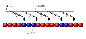
Figure 7: Schematic representation of the attachment sites. Each sphere represents an actin monomer; blue color delineate target zones.

Gaussian distribution of offsets. If we suppose that the distribution of axial offsets between the myosin head and the actin biding site is Gaussian we can estimate its standard deviation by noting that the probability that the variable deviation lies in the range $\pm k\sigma$ is given by,

$$\Pr(\mu-k\sigma\leq X\leq\mu+k\sigma)=\operatorname{erf}(\frac{k}{\sqrt{2}}),$$ (10)

we then use the fact that 60$\%$ is in the range $\pm$2.76nm to find $k=0.842$ and $\sigma=3.3$nm.

A.0.8 Critical response in soft and hard ensembles

In Fig. 8 we illustrate the mechanical responses in the adjacent critical regimes marked as $A$ and $B$ in Fig. 2 of the main text. In the associated critical points, indicated here by small circles and intended to represent the physiological regime of isometric contractions, the susceptibilities diverge. The closeness of these two regimes in the parameter space allows the system to exhibit the whole repertoire of behaviors from zero to infinite rigidity.

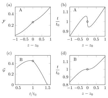
Figure 8: The response of the system in the critical regimes $A$ and $B$ shown in Fig. 2 of the main text : (a) and (b) are the Helmholtz free energy and the tension-elongation curve in the hard device ensemble; (c) and (d) are the Gibbs free energy and the associated tension-elongation curve in the soft device ensemble. Critical points are marked by the small circles.

A.0.9 Two half-sarcomeres in series

Here we present an elementary illustration of the fact that the equilibrium response of a bundle of contractile units connected in series and placed in a hard device, cannot be described by local equilibrium constitutive relations obtained in either soft or hard device ensembles. Instead, the system exhibits an intermediate behavior.

Consider two elementary contractile units in series, see Caruel and Truskinovsky (2018) for the analysis of $M$ such elements. Each of the two elements represents a parallel connection of $N$ cross-bridges. The total energy per cross bridge in dimensionless form for a system placed in a hard device reads

$$\begin{split}E_{2}=\frac{1}{2}\left\{\frac{1}{N}\sum_{i}^{N}[(1+x_{i1})v_{i1}+\frac{1}{2}(y_{1}-x_{i1})^{2}+\frac{\lambda_{f}}{2}(z_{1}-y_{1})^{2}]\right.\\ +\left.\frac{1}{N}\sum_{i}^{N}[(1+x_{i2})v_{i2}+\frac{1}{2}(y_{2}-x_{i2})^{2}+\frac{\lambda_{f}}{2}(z_{2}-y_{2})^{2}]\right\}\end{split}$$ (11)

The equilibrium response of the system is obtained by computing the partition function

$$\mathcal{Z}_{2}(z,\beta)=\int\exp[-2\beta NE_{2}]\delta(z_{1}+z_{2}-2z)d\bm{x}$$

where $d\bm{x}=\prod_{i}^{N}dx_{i1}dy_{1}\prod_{j}^{N}dx_{j2}dy_{2}$ and $z$ is the (average) elongation imposed on the system. We can rewrite the expression for $\mathcal{Z}_{2}$ in the form

$$\begin{split}\mathcal{Z}_{2}(z,\beta)=\int dy_{1}dy_{2}\exp\left\{-\beta N[-\frac{\lambda_{f}}{2}(z-y_{1}-y_{2})^{2}\right.\\ \left.-\frac{1}{\beta}\int dvp(v)\log\tilde{\mathcal{Z}}_{1}(y_{1},v)\tilde{\mathcal{Z}}_{2}(y_{2},v)]\right\}\end{split}$$ (12)

where $\tilde{\mathcal{Z}}_{i}(y_{i},v)=e^{-\frac{\beta}{2}(y_{i}+1)^{2}}+e^{-\beta(y_{i}^{2}/2+v)}$. The free energy per cross-bridge is then $\mathcal{F}_{2}(z,\beta)=-\frac{1}{2N}\log\mathcal{Z}_{2}(z,\beta)$. The equilibrium tension-elongation relation for this system, obtained from the relation $t(z,\beta)=\partial\mathcal{F}_{2}(z,\beta)/\partial z$, is shown by the thick line in Fig. 9(a). Similar thick line in Fig. 9(b) shows the equilibrium response of a single contractile element placed in the hard device.

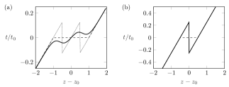
Figure 9: (a) Tension elongation relations for a system containing two half-sarcomeres in series placed in a hard device. Thick line: equilibrium response. Dotted (dashed) line: the response of two contractile elements in series, each one endowed with its own equilibrium the hard (soft) device constitutive law. (b) Response of a single half-sarcomere. Thick line: hard device; dashed line: soft device. $\beta=30$, $\sigma=0$, $v_{0}=0$, $\lambda_{f}=1$.

We now compare this behavior with the one obtained under the assumption that the two elements in series are characterized by their equilibrium free energies computed either in a hard or in a soft ensembles.

For instance, using the hard device ensemble we can write the total (Helmholtz) free energy of the two element system in the form $E_{2}^{hd}=\mathcal{F}(z_{1},\beta)+\mathcal{F}(z-z_{1},\beta)$, where $\mathcal{F}$ is the free energy of a half-sarcomere given by Eq. 5. The extra variable $z_{1}$ can be eliminated using the equilibrium condition $\partial\mathcal{F}(z_{1},\beta)/\partial z_{1}=\partial\mathcal{F}(z-z_{1},\beta)/\partial z_{1}$. The resulting tension elongation curve is shown in Fig. 9 (a) by a dotted line.

Similar analysis can be performed based on the response functions for the elements loaded in a soft device. Here we need to use equilibrium (Gibbs) free energies of the elements (Eq. 5 in the main text) and since the elements in series share the value of tension we obtain $G_{2}^{SD}=2\mathcal{G}(t,\beta)$. The ensuing response of the series bundle is shown in Fig. 9(a) by a dashed line. In Fig. 9(b), the dashed line show the equilibrium response of a single contractile element loaded in a soft device.

Observe, first, that the equilibrium response predicted by the two ’constitutive models’ contains discontinuities, while the response of the actually equilibrated system (two half-sarcomeres in series) is smooth. Note also that the actual response curves do not coincide with either of the two ’constitutive models’ and exhibit some intermediate behavior with features mimicking both models simultaneously. The observed discrepancy is due to the fact that in a fully equilibrated system none of the contractile elements is loaded in either soft or hard device and that the overal response of the system is fundamentally non-affine, see also Vilfan and Duke (2003); Caruel and Truskinovsky (2018).

References

- Huxley and Simmons (1971) A. F. Huxley and R. M. Simmons, Nature 233, 533 (1971).
- Caruel and Truskinovsky (2016) M. Caruel and L. Truskinovsky, Phys. Rev. E 93, 062407 (2016).
- Vilfan and Cowley (1985) I. Vilfan and R. A. Cowley, Journal of Physics C: Solid State Physics 18, 5055 (1985).
- Tregear et al. (1998) R. T. Tregear, R. J. Edwards, T. C. Irving, K. J. Poole, M. C. Reedy, H. Schmitz, E. Towns-Andrews, and M. K. Reedy, Biophysical Journal 74, 1439 (1998).
- Suzuki and Ishiwata (2011) M. Suzuki and S. Ishiwata, Biophysical Journal 101, 2740 (2011).
- Tregear et al. (2004) R. T. Tregear, M. C. Reedy, Y. E. Goldman, K. A. Taylor, H. Winkler, C. Franzini-Armstrong, H. Sasaki, C. Lucaveche, and M. K. Reedy, Biophysical Journal 86, 3009 (2004).
- Caruel and Truskinovsky (2018) M. Caruel and L. Truskinovsky, Reports on Progress in Physics 81, 036602 (2018).
- Vilfan and Duke (2003) A. Vilfan and T. Duke, Biophysical Journal 85, 191 (2003).