HQET form factors for ${\textnormal{B}_{\textnormal{s}}}\to\textnormal{K}\ell\nu$ decays beyond leading order

Abstract

We compute semi-leptonic ${\textnormal{B}_{\textnormal{s}}}$ decay form factors using Heavy Quark Effective Theory on the lattice. To obtain good control of the $1/m_{\textnormal{b}}$ expansion, one has to take into account not only the leading static order but also the terms arising at $\mathcal{O}\left(1/m_{\textnormal{b}}\right)$: kinetic, spin and current insertions. We show results for these terms calculated through the ratio method, using our prior results for the static order. After combining them with non-perturbative HQET parameters they can be continuum-extrapolated to give the QCD form factor correct up to $\mathcal{O}\left(1/m_{\textnormal{b}}^{2}\right)$ corrections and without $\mathcal{O}\left(\alpha_{s}(m_{\textnormal{b}})^{n}\right)$ corrections.

DESY 17-172

1 Introduction

Weak decays of B-mesons play an important role in determining the parameters of the Standard Model. In particular, the charmless charged-current semi-leptonic B decays, such as ${\textnormal{B}_{\textnormal{s}}}\to\textnormal{K}\ell\nu$, give a way to extract the poorly-constrained $|V_{\textnormal{ub}}|$ element of the CKM matrix.

The semi-leptonic ${\textnormal{B}_{\textnormal{s}}}\to\textnormal{K}\ell\nu$ decay is mediated by QCD matrix elements, which in the rest frame of the ${\textnormal{B}_{\textnormal{s}}}$ meson have the following form:

$$(2m_{\textnormal{B}_{\textnormal{s}}})^{-1/2}\langle\textnormal{K}(\mathbf{p}_{\textnormal{K}})|V^{0}(0)|{\textnormal{B}_{\textnormal{s}}}(0)\rangle =h_{\parallel}(E_{\textnormal{K}}),$$ (1)

$$(2m_{\textnormal{B}_{\textnormal{s}}})^{-1/2}\langle\textnormal{K}(\mathbf{p}_{\textnormal{K}})|V^{k}(0)|{\textnormal{B}_{\textnormal{s}}}(0)\rangle =p^{k}_{\textnormal{K}}h_{\perp}(E_{\textnormal{K}}),$$ (2)

where $\mathbf{p}_{\textnormal{K}}$ is the Kaon momentum and the vector current is defined as $V^{\mu}(x)=\overline{\psi}_{\rm u}(x)\gamma^{\mu}\psi_{\rm b}(x)$. Matrix elements $h_{\parallel}$ and $h_{\perp}$ are related to the often-used $f_{+}$, $f_{0}$ by simple kinematic relations, cf. Ref. Bahr:2016ayy .

Due to its large mass, the b quark requires special treatment to be discretized on the lattice without large cutoff effects. Our approach is to use Heavy Quark Effective Theory (HQET) Sommer:2015hea . Results at the leading order of HQET, the static approximation, are described in Bahr:2016ayy . There one can estimate the systematic error of the truncation of higher orders to be of order 15% – a number which is reduced to 1-2% when adding the $\mathcal{O}\left(1/m_{\textnormal{b}}\right)$ terms. It is therefore important to include these terms to obtain phenomenologically relevant results.

HQET expansion of a correlation function up to $\mathcal{O}\left(1/m_{\textnormal{b}}\right)$ is

$$\langle O\rangle=\langle O_{\textnormal{stat}}\rangle_{\textnormal{stat}}+\omega_{\textnormal{kin}}{\textstyle\sum}_{x}\langle O_{\textnormal{stat}}\mathcal{O}_{\textnormal{kin}}(x)\rangle_{\textnormal{stat}}+\omega_{\textnormal{spin}}{\textstyle\sum}_{x}\langle O_{\textnormal{stat}}\mathcal{O}_{\textnormal{spin}}(x)\rangle_{\textnormal{stat}}+{\textstyle\sum}_{\textnormal{k}}\omega_{\textnormal{k}}\langle O_{\textnormal{k}}\rangle_{\textnormal{stat}},$$ (3)

where $\mathcal{O}_{\textnormal{kin}}(x)=\overline{\psi}_{\textnormal{b}}(x)\mathbf{D}^{2}\psi_{\textnormal{b}}(x)$, $\mathcal{O}_{\textnormal{spin}}(x)=\overline{\psi}_{\textnormal{b}}(x)\,\bm{\sigma}\cdot\mathbf{B}\psi_{\textnormal{b}}(x)$ are the kinetic and spin terms, and $O_{\textnormal{k}}$ correspond to additional operators in the effective theory, which are discussed in Sec. 2.2. The (dimensionful) parameters of HQET $\omega_{\textnormal{spin}},\omega_{\textnormal{kin}},\omega_{\textnormal{k}}\propto 1/m_{\textnormal{b}}$ have to be determined by non-perturbative matching to QCD Heitger:2003nj ; DellaMorte:2013ega ; Sommer:2015hea . The notation $\langle\cdot\rangle_{\textnormal{stat}}$ means that the expectation values are defined with respect to the renormalizable static action.

For the computation of the matrix elements in the large volume we use $N_{\textnormal{f}}=2$ CLS ensembles Fritzsch:2012wq . Unless explicitly stated otherwise, all the results presented here were obtained on ensemble N6, with $a=0.048$ fm and $m_{\pi}=340$ MeV. The ${\textnormal{B}_{\textnormal{s}}}$ meson is kept at rest, while the Kaon has momentum $\mathbf{p}_{\textnormal{K}}=\frac{2\pi}{L}(1,0,0)$, which corresponds to $|\mathbf{p}_{\textnormal{K}}|=0.535$ GeV and the momentum transfer $q^{2}=21.23\;\textnormal{GeV}^{2}$. For more details on the ensembles used, see Ref. Bahr:2016ayy . The heavy quark is discretized using HYP1 action DellaMorte:2005yc and the light quarks are smeared with several levels of Gaussian smearing Gusken:1989ad ; Alexandrou:1990dq ; Bernardoni:2013xba .

2 Matrix elements at order $1/m_{\textnormal{b}}$

The HQET expansion up to order $1/m_{\textnormal{b}}$ of the heavy-light two-point correlation function is

$$\mathcal{C}^{\textnormal{B}_{\textnormal{s}}}(t)=\mathcal{C}^{\textnormal{B}_{\textnormal{s}}}_{\textnormal{stat}}(t)\left(1+\omega_{\textnormal{j}}\frac{\mathcal{C}^{\textnormal{B}_{\textnormal{s}}}_{\textnormal{j}}(t)}{\mathcal{C}^{\textnormal{B}_{\textnormal{s}}}_{\textnormal{stat}}(t)}\right),$$ (4)

where we schematically define $\mathcal{C}^{\textnormal{B}_{\textnormal{s}}}_{\textnormal{stat}}\equiv\langle P_{\textnormal{bs}}P_{\textnormal{sb}}\rangle_{\textnormal{stat}}$ and $\mathcal{C}^{\textnormal{B}_{\textnormal{s}}}_{\textnormal{j}}\equiv\langle P_{\textnormal{bs}}P_{\textnormal{sb}}\mathcal{O}_{\textnormal{j}}\rangle_{\textnormal{stat}}$ with $P_{\textnormal{q}_{1}\textnormal{q}_{2}}=\overline{\psi}_{\textnormal{q}_{1}}\gamma_{5}\psi_{\textnormal{q}_{2}}$ and $\textnormal{j}\in\{\textnormal{kin},\textnormal{spin}\}$.

The HQET expansion of the energy is $E^{\textnormal{B}_{\textnormal{s}}}=E^{\textnormal{B}_{\textnormal{s}}}_{\textnormal{stat}}+m_{\textnormal{bare}}+\omega_{\textnormal{kin}}E^{\textnormal{B}_{\textnormal{s}}}_{\textnormal{kin}}+\omega_{\textnormal{spin}}E^{\textnormal{B}_{\textnormal{s}}}_{\textnormal{spin}}$ Bernardoni:2013xba (in the following we suppress the ${\textnormal{B}_{\textnormal{s}}}$ index for readability). The contributions to the energy at the leading and next-to-leading order can be extracted from the large-time behaviour of the correlation functions:

$$-\partial_{t}\ln\mathcal{C}^{\textnormal{B}_{\textnormal{s}}}_{\textnormal{stat}}(t)=E_{\textnormal{stat}}+\mathcal{O}\left(e^{-\Delta Et}\right),$$ (5)

$$-\partial_{t}\frac{\mathcal{C}^{\textnormal{B}_{\textnormal{s}}}_{\textnormal{j}}(t)}{\mathcal{C}^{\textnormal{B}_{\textnormal{s}}}_{\textnormal{stat}}(t)}=E_{\textnormal{j}}+\mathcal{O}\left(te^{-\Delta Et}\right).$$ (6)

The three-point correlation functions, $\mathcal{C}^{\textnormal{3pt}}_{\mu,\textnormal{stat}}\equiv\langle P_{\textnormal{su}}V^{\mu}P_{\textnormal{bs}}\rangle_{\textnormal{stat}}$, can also be used to obtain the energy contributions:

$$-\partial_{t_{\textnormal{B}_{\textnormal{s}}}}\frac{\mathcal{C}^{\textnormal{3pt}}_{\mu,\textnormal{j}}({t_{\textnormal{K}}},{t_{\textnormal{B}_{\textnormal{s}}}})}{\mathcal{C}^{\textnormal{3pt}}_{\mu,\textnormal{stat}}({t_{\textnormal{K}}},{t_{\textnormal{B}_{\textnormal{s}}}})}=E_{\textnormal{j}}+\mathcal{O}\left({t_{\textnormal{B}_{\textnormal{s}}}}e^{-\Delta E{t_{\textnormal{B}_{\textnormal{s}}}}}\right).$$ (7)

From here on, for simplicity, we set that ${t_{\textnormal{K}}}={t_{\textnormal{B}_{\textnormal{s}}}}=t$ and drop the second argument in the three-point functions and ratios.

After integrating the equations at order $1/m_{\textnormal{b}}$ we obtain

$$\frac{\mathcal{C}^{\textnormal{B}_{\textnormal{s}}}_{\textnormal{j}}(t)}{\mathcal{C}^{\textnormal{B}_{\textnormal{s}}}_{\textnormal{stat}}(t)}=A_{\textnormal{j}}-E_{\textnormal{j}}t+\mathcal{O}\left(te^{-\Delta Et}\right),$$ (8)

$$\frac{\mathcal{C}^{\textnormal{3pt}}_{\mu,\textnormal{j}}(t)}{\mathcal{C}^{\textnormal{3pt}}_{\mu,\textnormal{stat}}(t)}=A_{\mu,\textnormal{j}}^{\textnormal{3pt}}-E_{\textnormal{j}}t+\mathcal{O}\left(te^{-\Delta Et}\right),$$ (9)

where $A$ are the integration constants, which depend on the smearing used (for notational clarity we keep the smearing indices implicit).

We define two ratios from which we can obtain the desired bare matrix elements:

$$\mathcal{R}^{\textnormal{I}}_{\mu}(t)= \frac{\mathcal{C}^{\textnormal{3pt}}_{\mu}(t)}{\big{[}\mathcal{C}^{\textnormal{K}}(2t)\mathcal{C}^{\textnormal{B}_{\textnormal{s}}}(2t)\big{]}^{1/2}},$$ (10)

$$\mathcal{R}^{\textnormal{II}}_{\mu}(t)= \frac{\mathcal{C}^{\textnormal{3pt}}_{\mu}(t)}{\big{[}\mathcal{C}^{\textnormal{K}}(t)\mathcal{C}^{\textnormal{B}_{\textnormal{s}}}(t)\big{]}^{1/2}}e^{(\bar{E}^{\textnormal{K}}+\bar{E}^{\textnormal{B}_{\textnormal{s}}})\frac{t}{2}},$$ (11)

where for precision we set the effective energies $\bar{E}^{\textnormal{K}},\bar{E}^{\textnormal{B}_{\textnormal{s}}}$ to their ground-state values as extracted from the plateaux and GEVP plateaux respectively. This reduces the statistical error compared to the time-dependent effective energies at the expense of any systematic error in the determination of the energies propagating into the ratios. However, the ground-state energies are well under control.

Let us start with ratio $\mathcal{R}^{\textnormal{I}}$ which is simpler theoretically, because it requires no extra input apart from the correlation functions, but has larger statistical errors, due to the use of the heavy-light two-point function at time separation $2t$.

In the following, we use the symbol $\cong$ for relations which hold in the asymptotic large-time limit and up to terms of $\mathcal{O}\left(1/m_{\textnormal{b}}^{2}\right)$. HQET expansion of the ratio is

$$\mathcal{R}^{\textnormal{I}}_{\mu}(t)\cong\mathcal{R}^{\textnormal{I}}_{\mu,\textnormal{stat}}(t)\left[1+\omega_{\textnormal{j}}\left(\frac{\mathcal{C}^{\textnormal{3pt}}_{\mu,\textnormal{j}}(t)}{\mathcal{C}^{\textnormal{3pt}}_{\mu,\textnormal{stat}}(t)}-\frac{1}{2}\frac{\mathcal{C}^{\textnormal{B}_{\textnormal{s}}}_{\textnormal{j}}(2t)}{\mathcal{C}^{\textnormal{B}_{\textnormal{s}}}_{\textnormal{stat}}(2t)}\right)+\omega_{\textnormal{k}}\frac{\mathcal{C}^{\textnormal{3pt}}_{\mu,\textnormal{k}}(t)}{\mathcal{C}^{\textnormal{3pt}}_{\mu,\textnormal{stat}}(t)}\right]\equiv\mathcal{R}^{\textnormal{I}}_{\mu,\textnormal{stat}}(t)\left[1+\omega_{\textnormal{j}}\rho^{\textnormal{I}}_{\mu,\textnormal{j}}+\omega_{\textnormal{k}}\rho_{\mu,\textnormal{k}}\right],$$ (12)

where j is implicitly summed over $\{\textnormal{kin},\textnormal{spin}\}$ and k over the additional vector-current contributions, see Sec. 2.2. At large times $\rho$-s correspond to the $1/m_{\textnormal{b}}$ corrections to the bare HQET matrix elements.

The same procedure can be applied to $\mathcal{R}^{\textnormal{II}}$:

$$\mathcal{R}^{\textnormal{II}}_{\mu}(t)\cong \,\mathcal{R}^{\textnormal{II}}_{\mu,\textnormal{stat}}(t)\left[1+\omega_{\textnormal{j}}\left(\frac{\mathcal{C}^{\textnormal{3pt}}_{\mu,\textnormal{j}}(t)}{\mathcal{C}^{\textnormal{3pt}}_{\mu,\textnormal{stat}}(t)}-\frac{1}{2}\frac{\mathcal{C}^{\textnormal{B}_{\textnormal{s}}}_{\textnormal{j}}(t)}{\mathcal{C}^{\textnormal{B}_{\textnormal{s}}}_{\textnormal{stat}}(t)}+\frac{E_{\textnormal{j}}t}{2}\right)+\omega_{\textnormal{k}}\rho_{\mu,\textnormal{k}}\right]$$ (13)

$$\cong \,\mathcal{R}^{\textnormal{II}}_{\mu,\textnormal{stat}}(t)\left[1+\omega_{\textnormal{j}}\left(\frac{\mathcal{C}^{\textnormal{3pt}}_{\mu,\textnormal{j}}(t)}{\mathcal{C}^{\textnormal{3pt}}_{\mu,\textnormal{stat}}(t)}-\frac{\mathcal{C}^{\textnormal{B}_{\textnormal{s}}}_{\textnormal{j}}(t)}{\mathcal{C}^{\textnormal{B}_{\textnormal{s}}}_{\textnormal{stat}}(t)}+\frac{A_{\textnormal{j}}}{2}\right)+\omega_{\textnormal{k}}\rho_{\mu,\textnormal{k}}\right],$$ (14)

where Eq. (13) and Eq. (14) are related by Eq. (8). Analogously to the previous case we label the coefficients multiplying $\omega_{\textnormal{j}}$ as $\rho^{\textnormal{II}}_{\mu,\textnormal{j}}$. Note that both methods of calculating $\rho^{\textnormal{II}}_{\mu,\textnormal{j}}$ require extra input (either $E_{\textnormal{j}}$ or $A_{\textnormal{j}}$) that must be obtained through a fit, as described in the following subsection.

In addition, we note that there is one additional contribution to the matrix elements at the 1/m level coming from an overall multiplicative renormalization to the ratios $\mathcal{R}^{\textnormal{I}}$ and $\mathcal{R}^{\textnormal{II}}$, we refer the interested reader to Refs. Sommer:2015hea ; Heitger:2003nj for details.

2.1 Results for the kinetic and spin insertions

At large enough time, for each j separately, both ratios must plateau at the same value, from which we obtain the desired $1/m_{\textnormal{b}}$ matrix-element contribution. Using Eqs. (8)-(9), it can be also written as

$$\rho^{\textnormal{I}}_{\mu,\textnormal{j}}(t)\cong\rho^{\textnormal{II}}_{\mu,\textnormal{j}}(t)\cong A^{\textnormal{3pt}}_{\mu,\textnormal{j}}-A_{\textnormal{j}}/2.$$ (15)

Note that, while both $A_{\textnormal{j}}$, $A^{\textnormal{3pt}}_{\mu,\textnormal{j}}$ depend on the smearing, their combination in Eq. (15) does not.

Figure 1: The example result of the simultaneous fit procedure for the spin insertions.

We can extract $A_{\textnormal{j}}$, $A^{\textnormal{3pt}}_{\mu,\textnormal{j}}$ from fitting Eqs. (8) and (9). We choose to do a simultaneous fit to both the equations, and both $\mu=0$ and 1. In this way we are utilizing the fact that the linear slope (given by the energy contribution $E_{\textnormal{j}}$) is common in all of them. We find that this significantly improves the precision that we can obtain, especially for the particularly demanding $A^{\textnormal{3pt}}_{\mu=1,\textnormal{j}}$. An illustration is given in Fig. 1. We use the fit range $t\in[0.8\leavevmode\nobreak\ \textnormal{fm},1.4\leavevmode\nobreak\ \textnormal{fm}]$.

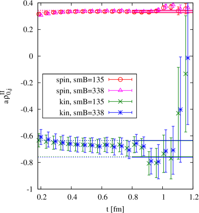
Figure 2: Kinetic and spin insertions for $\mu=0$ (left) and $\mu=1$ (right) from the ratios and fits, for two different amounts of light-quark smearing. The data for different smearings are slightly shifted horizontally for greater visibility.

In Fig. 2 we show the comparison of $\rho^{\textnormal{II}}_{\mu,\textnormal{j}}(t)$, calculated using Eq. (14) with the $A_{\textnormal{j}}$ from the simultaneous fit (one can also calculate $A_{\textnormal{j}}$ from the two-point functions only, the results are perfectly consistent and have slightly larger errorbars). We also show the bands coming from the fits. A good agreement between different light-quark smearings is observed. In addition, the fit results for the highest smearing are collected in Table 1.

$\mu$	$\rho^{\textnormal{II}}_{\mu,\textnormal{kin}}$
0	-0.70(6)
1	-0.81(7)

$\mu$	$\rho^{\textnormal{II}}_{\mu,\textnormal{spin}}$
0	0.338(7)
1	-0.189(8)

Table 1: Fit results for the kin (left) and spin (right) contributions at the highest light-quark smearing.

The uncertainty of the kin contribution is dominant. Note, however, that the previously determined subset of the HQET parameters Blossier:2012qu yields for $\omega_{\textnormal{spin}}$ a value which is approximately two times larger than for $\omega_{\textnormal{kin}}$, therefore the overall contribution and uncertainty of the two channels is more comparable.

2.2 Vector current insertions

$\mu$	k	$V_{\mu,\textnormal{k}}$	$\omega^{\textnormal{tree}}_{\mu,\textnormal{k}}\cdot m_{\textnormal{b}}$	$\rho_{\mu,\textnormal{k}}$
0	1	$\overline{\psi}_{\ell}(x)\sum_{l}\gamma_{l}\tfrac{1}{2}(\nabla_{l}^{\textnormal{S}}-\overleftarrow{\nabla}_{l}^{\textnormal{S}})\psi_{\textnormal{b}}(x)$	1/2	-0.0730(13)
0	2	$\overline{\psi}_{\ell}(x)\sum_{l}\gamma_{l}\tfrac{1}{2}(\nabla_{l}^{\textnormal{S}}+\overleftarrow{\nabla}_{l}^{\textnormal{S}})\psi_{\textnormal{b}}(x)$	1/2	-0.0284$(\phantom{0}3)$
$i$	1	$\overline{\psi}_{\ell}(x)\sum_{l}\tfrac{1}{2}(\nabla_{l}^{\textnormal{S}}-\overleftarrow{\nabla}_{l}^{\textnormal{S}})\gamma_{l}\gamma_{i}\psi_{\textnormal{b}}(x)$	1/2	0.3232(26)
$i$	2	$\overline{\psi}_{\ell}(x)\tfrac{1}{2}(\nabla_{i}^{\textnormal{S}}-\overleftarrow{\nabla}_{i}^{\textnormal{S}})\psi_{\textnormal{b}}(x)$	-1	0.0869(17)
$i$	3	$\overline{\psi}_{\ell}(x)\sum_{l}\tfrac{1}{2}(\nabla_{l}^{\textnormal{S}}+\overleftarrow{\nabla}_{l}^{\textnormal{S}})\gamma_{l}\gamma_{i}\psi_{\textnormal{b}}(x)$	1/2	0.1083(12)
$i$	4	$\overline{\psi}_{\ell}(x)\tfrac{1}{2}(\nabla_{i}^{\textnormal{S}}+\overleftarrow{\nabla}_{i}^{\textnormal{S}})\psi_{\textnormal{b}}(x)$	-1	0.1083(12)

Table 2: Overview of the vector current insertions in HQET at $\mathcal{O}\left(1/m_{\textnormal{b}}\right)$, their corresponding tree-level matching coefficients, and the results at the highest light-quark smearing. $\nabla^{S}_{i}$ are symmetric lattice derivatives.

Additional terms at $\mathcal{O}\left(1/m_{\textnormal{b}}\right)$ to the vector current are

$$V_{0}^{\mathrm{HQET}}(x)=Z_{V_{0}}^{\mathrm{HQET}}\big{(}V_{0}^{\mathrm{stat}}(x)+{\textstyle\sum}_{\textnormal{k}=1}^{2}\omega_{0,\textnormal{k}}V_{0,\textnormal{k}}(x)\big{)},$$ (16)

$$V_{i}^{\mathrm{HQET}}(x)=Z_{V_{i}}^{\mathrm{HQET}}\big{(}V_{i}^{\mathrm{stat}}(x)+{\textstyle\sum}_{\textnormal{k}=1}^{4}\omega_{i,\textnormal{k}}V_{i,\textnormal{k}}(x)\big{)}$$ (17)

where the operators used are summarized in Table 2. Note that with our choice of momentum, along the $x$-axis, only $i=1$ contributes. Also, for this choice of momentum the large-volume matrix elements arising from $V_{1,3}$ and $V_{1,4}$ are identical.

The results obtained are presented in Fig. 3. We see clear plateaux starting at roughly 0.8-0.9 fm and the precision is better than that of the kin and spin terms. A full quantitative comparison has to wait until the corresponding non-perturbative matching coefficients are available.

Figure 3: Overview of the current insertions. Fit bands are plateaux averages starting at 0.86 fm.

3 Summary & outlook

Figure 4: Absolute values of bare matrix-elements contributions, multiplied by their corresponding tree-level coefficients, as a function of the lattice spacing on CLS ensembles A5, F6 and N6 Fritzsch:2012wq . All the ensembles have a similar pion mass and the momentum transfer on the coarser ensembles has been tuned to match that of N6 by using twisted boundary conditions, cf. Ref. Bahr:2016ayy . Note that $1/a$ divergences are not removed in those bare quantities. Only after combining with the non-perturbative matching results, the continuum limit can be taken. The data for different $\mu$ are slightly shifted horizontally for greater visibility.

Let us first give a graphical summary of the obtained results. The extracted $1/m_{\textnormal{b}}$ contributions as a function of the lattice spacing on three CLS ensembles is given in Fig 4. In the current form, the continuum limit cannot be taken, as divergences will only be removed once the non-perturbative matching coefficients are known.

The overall precision is limited by the signal-to-noise problem, the signal rapidly deteriorates above 1.2 fm. For the kin and spin contributions the matching coefficients are available, therefore one can give a rough estimate of the obtained precision, which we expect to be at the level of 3% of the final result. This is comparable to the precision of our previously obtained static results Bahr:2016ayy .

For the $1/m_{\textnormal{b}}$ corrections to the vector current the large-volume matrix elements $\rho_{\mu,\textnormal{k}}$ themselves are determined with an absolute precision between $3\times 10^{-4}$ and $3\times 10^{-3}$. This will give a sub-percent contribution to the uncertainty of the final result, unless the corresponding non-perturbative matching coefficients have unnaturally high values.

In other words, the computation of the $1/m_{\textnormal{b}}$ terms is not the most challenging part in the determination of the form factors. The same pattern for the $1/m_{\textnormal{b}}$ corrections was seen before in simpler quantities Bernardoni:2013xba ; Bernardoni:2014fva ; Bernardoni:2015nqa .

A further significant improvement of the precision in the presence of an exponential signal-to-noise problem is not an easy task. Some gain can certainly be obtained by using momentum smearing Bali:2016lva . Another promising direction is to use a multi-level algorithm along the lines of Refs. Ce:2016idq ; Ce:2016ajy .

References

(1)
F. Bahr, D. Banerjee, F. Bernardoni et al. (ALPHA), Phys. Lett. B757,
473 (2016), 1601.04277
(2)
R. Sommer, Nucl. Part. Phys. Proc. 261-262, 338 (2015),
1501.03060
(3)
J. Heitger, R. Sommer (ALPHA), JHEP 02, 022 (2004),
hep-lat/0310035
(4)
M. Della Morte, S. Dooling, J. Heitger, D. Hesse, H. Simma (ALPHA), JHEP
05, 060 (2014), 1312.1566
(5)
P. Fritzsch, F. Knechtli, B. Leder et al., Nucl. Phys. B865, 397
(2012), 1205.5380
(6)
M. Della Morte, A. Shindler, R. Sommer, JHEP 0508, 051 (2005),
hep-lat/0506008
(7)
S. Güsken, U. Löw, K.H. Mütter et al., Phys. Lett. B227,
266 (1989)
(8)
F. Bernardoni et al., Phys. Lett. B730, 171 (2014), 1311.5498
(9)
C. Alexandrou, F. Jegerlehner, S. Güsken, K. Schilling, R. Sommer, Phys.
Lett. B256, 60 (1991)
(10)
B. Blossier, M. Della Morte, P. Fritzsch et al. (ALPHA), JHEP 09, 132
(2012), 1203.6516
(11)
F. Bernardoni et al. (ALPHA), Phys. Lett. B735, 349 (2014),
1404.3590
(12)
F. Bernardoni, B. Blossier, J. Bulava et al., Phys. Rev. D92, 054509
(2015), 1505.03360
(13)
G.S. Bali, B. Lang, B.U. Musch, A. SchÃfer, Phys. Rev. D93, 094515
(2016), 1602.05525
(14)
M. CÃ, L. Giusti, S. Schaefer, Phys. Rev. D93, 094507 (2016),
1601.04587
(15)
M. CÃ, L. Giusti, S. Schaefer, Phys. Rev. D95, 034503 (2017),
1609.02419