Error estimates for extrapolations with matrix-product states

Abstract

We introduce a new error measure for matrix-product states without requiring the relatively costly two-site density matrix renormalization group (2DMRG). This error measure is based on an approximation of the full variance $\langle\psi|(\hat{H}-E)^{2}|\psi\rangle$. When applied to a series of matrix-product states at different bond dimensions obtained from a single-site density matrix renormalization group (1DMRG) calculation, it allows for the extrapolation of observables towards the zero-error case representing the exact ground state of the system. The calculation of the error measure is split into a sequential part of cost equivalent to two calculations of $\langle\psi|\hat{H}|\psi\rangle$ and a trivially parallelized part scaling like a single operator application in 2DMRG. The reliability of the new error measure is demonstrated at four examples: the $L=30,S=\nicefrac{{1}}{{2}}$ Heisenberg chain, the $L=50$ Hubbard chain, an electronic model with long-range Coulomb-like interactions and the Hubbard model on a cylinder of size $10\times 4$. Extrapolation in the new error measure is shown to be on-par with extrapolation in the 2DMRG truncation error or the full variance $\langle\psi|(\hat{H}-E)^{2}|\psi\rangle$ at a fraction of the computational effort.

I Introduction

The density matrix renormalization groupWhite (1992); Schollwöck (2011) (DMRG) method and its underlying matrix-product state (MPS) structure are the method of choice for ground-state search and representation of one-dimensional quantum states. In the last few years, it has also been applied to wider and wider cylindrical systemsWhite and Scalapino (2004, 2009); Depenbrock et al. (2012); Yan et al. (2011); Ehlers et al. (2017); Motruk et al. (2016) to mimic two-dimensional physics. Furthermore, methods relying on the precise solution of a small effective system, such as the dynamical mean-field theoryGeorges and Kotliar (1992); Karski et al. (2008); Ganahl et al. (2015); Wolf et al. (2015); Bauernfeind et al. (2017) (with or without a dynamical cluster approximation) or the density matrix embedding theoryKnizia and Chan (2013) have also started to use DMRG to solve the effective problem resulting from the embedding. Growing computational resources as well as algorithmic improvements made the study of critical systemsWhite and Affleck (1996); Yamashita et al. (1998); Andersson et al. (1999); Vidal et al. (2003); Vidal (2007); Chen et al. (2015); Khait et al. (2017) in one dimension also more feasible.

In those complex systems it is often not possible to increase the precision of the matrix-product state ansatz sufficiently to capture the ground state of the system exactly. Instead, one often measures both the observables of interest, among them the energy, and the truncation error as obtained from a two-site DMRG (2DMRG) calculation during the calculation and at various precisions. One may then extrapolateLegeza and Fáth (1996); White (2005); LeBlanc et al. (2015); Ehlers et al. (2017) the measured observables towards zero truncation error to obtain a comparably accurate estimate of the ground-state observable. This truncation error can also be obtained from a traditional environment-site-site-environment DMRG procedure which is equivalent to the MPS-based 2DMRG method.

Unfortunately, the 2DMRG method is relatively computationally expensive,Hubig et al. (2015) scales relatively badly in the local physical dimensionDorfner (2017) and it is sometimes slow to pick up long-range correlations.White (2005) It would hence be preferable to only use single-site DMRG (1DMRG, corresponding to a environment-site-environment setup in the traditional DMRG) for an approximately four-fold computational speed-up in spin and fermionic systems and a much larger speed-up in bosonic systems. The subspace expansion schemeHubig et al. (2015) for 1DMRG does not yield a usable truncation error. The related density matrix perturbationWhite (2005) again scales relatively badly in the local physical dimension.

Measuring the full variance $\langle\psi|(\hat{H}-E)^{2}|\psi\rangle$ would provide a reliable error measurement for 1DMRG but is computationally very costly and often impossible to evaluate even if expectation value measurements and single-site DMRG calculations are still feasible. This is in particular true for large systems with long-range interactions or an underlying two-dimensional structure. Since such systems typically result in highly entangled ground states and hence require large computational resources per se, minimization of these resources wherever possible is key.

For these reasons, we wish to formulate a method which measures an error quantity $\mathit{err}(|\psi\rangle,\hat{H})$ based only on a matrix-product state $|\psi\rangle$ (regardless of how it was obtained) and associated Hamiltonian $\hat{H}$. Measuring this error as well as an observable for different states should allow an extrapolation of the observable towards zero error. Evaluating the error measure should not be much more costly than a 1DMRG calculation. We find that the 2-site variance, an approximation of the full variance, fulfills these requirements and turns 1DMRG into a fast method with a controlled extrapolation scheme even for complex systems.

The rest of the paper is structured as follows: In Sec. II we briefly review MPS and the related matrix-product operator (MPO) notation. Sec. III discusses the currently available error measures. Sec. IV explains the new approximation of the variance to serve as the new error measure. In Sec. V, we consider four relevant examples to show that the variance itself is an error measure suitable for extrapolations, that the 2-site approximation of the variance is also a valid extrapolation tool even if it does not coincide with the variance and finally that the 2-site variance is also applicable in two-dimensional systems where evaluation of the full variance is not possible any more. The conclusions in Sec. VI serve as a brief summary.

Figure 1: Top: Graphical representation of a MPS in mixed-canonical form with the orthogonality center on site 3 and tensors $A_{1},A_{2},M_{3},B_{4},B_{5}$. Explicit tensor and tensor leg labels are given here. Bottom: Conditions for left and right-normalized tensors to result in identity matrices upon contraction. Labels are left off to avoid clutter.

II MPS and MPO notation

Matrix-product states (MPS) describe quantum mechanical states on a separable Hilbert space $\mathcal{H}=\otimes_{i=1}^{L}\mathcal{H}_{i}$, each with a local basis $\left\{|\sigma_{i}\rangle\right\}_{\sigma_{i}=1}^{d_{i}}$. To represent a state $|\psi\rangle$, $L$ rank-3 tensors $M_{i;m_{i}}^{\sigma_{i}m_{i-1}}$ are selected such that

$$|\psi\rangle=\sum_{\sigma_{1}}\ldots\sum_{\sigma_{L}}M_{1;m_{1}}^{\sigma_{1}m_{0}}\cdots M_{L;m_{L}}^{\sigma_{1}m_{L-1}}|\sigma_{L}\ldots\sigma_{L}\rangle\quad.$$ (1)

Here, the $\cdot$ represents a contraction of the tensors over all common indices, i.e.

$$M_{1;m_{1}}^{\sigma_{1}m_{0}}\cdot M_{2;m_{2}}^{\sigma_{2}m_{1}}=\sum_{m_{1}}M_{1;m_{1}}^{\sigma_{1}m_{0}}M_{2;m_{2}}^{\sigma_{2}m_{1}}\quad.$$ (2)

The $m_{i}$ are called right MPS bond indices, $m_{i-1}$ are the left MPS bond indices and $\sigma_{i}$ are the local physical indices. $m_{0}$ and $m_{L}$ are one-dimensional dummy indices inserted for consistency. It is useful to differentiate between incoming (lower, bra) and outgoing (upper, ket) indices in the context of implementing symmetries in the network. An incoming index may only be contracted with an outgoing index and vice-versa. Indices may be left off if they are clear from context, e.g.:

$$M_{1}\cdot M_{2}=\sum_{m_{1}}M_{1;m_{1}}^{\sigma_{1}m_{0}}M_{2;m_{2}}^{\sigma_{2}m_{1}}\quad.$$ (3)

Furthermore, we will write $\boldsymbol{\sigma}$ to refer to all $\sigma_{1},\ldots,\sigma_{L}$.

Matrix-product state tensors may optionally be left- or right-normalized. ‘A’ instead of ‘M’ will be used for left-normalized tensors which fulfill

$$\sum_{\sigma_{i},m_{i-1}}A_{i;m_{i}}^{\sigma_{i}m_{i-1}}A_{i;\sigma_{i}m_{i-1}}^{\dagger;\tilde{m}_{i}}=\mathbf{1}_{m_{i}}^{\tilde{m}_{i}}$$ (4)

and ‘B’ will be used for right-normalized tensors fulfilling

$$\sum_{\sigma_{i},m_{i}}B_{i;m_{i}}^{\sigma_{i}m_{i-1}}B_{i;\sigma_{i}\tilde{m}_{i-1}}^{\dagger;m_{i}}=\mathbf{1}^{m_{i-1}}_{\tilde{m}_{i-1}}\quad,$$ (5)

where ^† denotes complex conjugation of all entries and reversal of index directions such that $A_{i;\sigma_{i}m_{i-1}}^{\dagger;\tilde{m}_{i}}\equiv\big{(}A_{i}^{\dagger}\big{)}_{\sigma_{i}m_{i-1}}^{\tilde{m}_{i}}=\left[A_{i;m_{i}}^{\sigma_{i}m_{i-1}}\right]^{\star}$. A matrix-product state is in left-canonical (right-canonical) form if all tensors are left-normalized (right-normalized). A matrix-product state in which all tensors to the left of a specific site $k$ are left-normalized and all tensors to the right of that site $k$ are right-normalized is in mixed-canonical formSchollwöck (2011) and site $k$ is its orthogonality centerStoudenmire and White (2010) (cf. Fig. 1).

In a similar fashion, operators may be written as matrix-product operators, consisting of $L$ rank-4 tensors $W_{i;\sigma_{i}w_{i}}^{\tau_{i}w_{i-1}}$, such that:

$$\hat{H}=\sum_{\boldsymbol{\sigma}\boldsymbol{\tau}}W_{1}\cdot W_{2}\cdots W_{L}|\boldsymbol{\tau}\rangle\langle\boldsymbol{\sigma}|\quad.$$ (6)

Just like MPS tensors, MPO tensors have a left MPO bond index ($w_{i-1}$), a right MPO bond index ($w_{i}$) as well as an upper and lower physical index ($\tau_{i}$ and $\sigma_{i}$ resp.). Multiple methods to construct MPOs from scratch exist.Chan et al. (2016); Hubig et al. (2017); Paeckel et al. (2017)

Figure 2: Consecutive left- and right-contractions of the MPO (squares) sandwiched between normalized MPS tensors (triangles). $L_{0}$ and $R_{L+1}$ are the dummy tensors inserted for consistency. Connecting any pair $L_{i}\cdot R_{i+1}$ results in the expectation value of the operator.

The following definitions will be useful later (cf. Fig. 2):

$$L_{0} =\mathbf{1}^{\tilde{m}_{0}}_{w_{0}m_{0}}$$ (7)

$$L_{i} =L_{i-1}\cdot W_{i}\cdot A_{i}\cdot A_{i}^{\dagger}$$ (8)

$$R_{L+1} =\mathbf{1}^{w_{L}m_{L}}_{\tilde{m}_{L}}$$ (9)

$$R_{i} =R_{i+1}\cdot W_{i}\cdot B_{i}\cdot B_{i}^{\dagger}$$ (10)

The $L_{i}$ and $R_{i}$ are the usual left and right contractions of the Hamiltonian sandwiched between the state as encountered during standard DMRG, standard TDVPHaegeman et al. (2016) or expectation value calculations. Hence, we can expect to be able to calculate them efficiently. As a visualization, note that

$$L_{i}\cdot R_{i+1}=\langle\psi|\hat{H}|\psi\rangle\quad\forall i\in[0,L]\quad.$$ (11)

Throughout this paper, we will use $m$, $w$ and $d$ to denote the effective MPS bond dimension, the effective MPO bond dimension and the effective size of the local basis in particular when estimating the computational cost of an operation.

Given an MPS tensor $A_{i}$, we can view it as an orthonormal basis transformation and truncation from an effective left basis ($m_{i-1}$) and local basis ($\sigma_{i}$) into a new effective right basis ($m_{i}$). However, the new right-hand side basis will typically not span the complete space reachable from $m_{i-1}\otimes\sigma_{i}$, but only a small subset thereof with size $m_{i}$. We hence define tensors $F_{i}$ (and conversely $G_{i}$ when working with $B_{i}$) which reach the additional $(d-1)m$ states with the properties

$$\sum_{\sigma_{i},m_{i-1}}A_{i;m_{i}}^{\sigma_{i}m_{i-1}}F_{i;\sigma_{i}m_{i-1}}^{\dagger;\tilde{m}^{\prime}_{i}}=0$$ (12)

$$\sum_{\sigma_{i},m_{i-1}}F_{i;m^{\prime}_{i}}^{\sigma_{i}m_{i-1}}F_{i;\sigma_{i}m_{i-1}}^{\dagger;\tilde{m}^{\prime}_{i}}=\mathbf{1}_{m^{\prime}_{i}}^{\tilde{m}^{\prime}_{i}}$$ (13)

and equivalently for $G_{i}$:

$$\sum_{\sigma_{i},m_{i}}B_{i;m_{i}}^{\sigma_{i}m_{i-1}}G_{i;\sigma_{i}\tilde{m}^{\prime}_{i-1}}^{\dagger;m_{i}}=0$$ (14)

$$\sum_{\sigma_{i},m_{i}}G_{i;m_{i}}^{\sigma_{i}m^{\prime}_{i-1}}G_{i;\sigma_{i}\tilde{m}^{\prime}_{i-1}}^{\dagger;m_{i}}=\mathbf{1}_{\tilde{m}^{\prime}_{i-1}}^{m^{\prime}_{i-1}}$$ (15)

When interpreting $A_{i;m_{i}}^{\sigma_{i}m_{i-1}}$ as a rectangular matrix whose row index is obtained from joining the left virtual and physical index (i.e. the two upper indices), it is an isometric matrix in the sense of Eq. (4). Similarly interpreting $F_{i;m^{\prime}_{i}}^{\sigma_{i}m_{i-1}}$, it corresponds to the additional columns required to extend the isometric matrix $A_{i}$ into a square unitary matrix. Put differently, if $A_{i}$ is obtained from a ‘reduced’ or ‘thin’ QR decomposition, one can similarly obtain $F_{i}$ by instead requesting a ‘full’ decomposition with a square and unitary Q matrix of size $md\times md$ (assuming that the left bond dimension is $m$). The first $m$ columns correspond to $A_{i;m_{i}}^{\sigma_{i}m_{i-1}}$, whereas the last $m(d-1)$ columns define $F_{i;m^{\prime}_{i}}^{\sigma_{i}m_{i-1}}$, with thus $m^{\prime}_{i}=1,\ldots,m(d-1)$. An analogous construction defines $G_{i;m_{i}}^{\sigma_{i}m^{\prime}_{i-1}}$.

III Current alternatives

III.1 2DMRG truncation error

The 2DMRG truncation error is readily available from a 2DMRG calculation and has repeatedly been shownLegeza and Fáth (1996); White (2005); LeBlanc et al. (2015); Ehlers et al. (2017) to allow a reliably extrapolation of observables obtained during the calculation towards the infinite-precision ground state. In the examples later in the paper, we have taken the largest 2DMRG truncation error and the lowest eigensolver energy encountered during the last half-sweep at a given bond dimension as error measure and expectation value respectively.

However, the 2DMRG method both scales relatively badly in the local physical dimension as $O(m^{3}d^{2}w+m^{2}d^{3}w^{2}+m^{3}d^{3})$ and sometimes – in particular, if no noise terms are used – is slow to pick up long-range correlations.White (2005) Generally, one can expect a speed-up of approximately four in fermionic or spin systems when switching to a single-site implementation to obtain the same accuracy in energy.Hubig et al. (2015) Furthermore, the idea of updating two sites at the same time runs somewhat counter to the original aim of matrix-product states, namely reducing the exponential complexity of the Hilbert space as much as possible. Finally, the 2DMRG truncation error is obtained during the 2DMRG calculation and hence applies to the DMRG process itself, not necessarily to the resulting state. If the state is already well-converged at the current bond dimension and hence changes little in subsequent sweeps, the difference will be minimal and the extrapolation can be applied correctly. However, it may be difficult to pinpoint this convergence during a large-scale calculation.

III.2 The full variance

Evaluation of the full variance $\langle\psi|\hat{H}^{2}|\psi\rangle-\langle\psi|\hat{H}|\psi\rangle^{2}$ directly yields information on the non-eigenstate content of the (assumed normalized) state $|\psi\rangle$: With $E=\langle\psi|\hat{H}|\psi\rangle$, the residuum $|\phi\rangle$ is given as

$$|\phi\rangle =\hat{H}|\psi\rangle-E|\psi\rangle$$ (16)

$$\Rightarrow\langle\phi|\phi\rangle =\langle\psi|\hat{H}^{2}|\psi\rangle-E^{2}\quad.$$ (17)

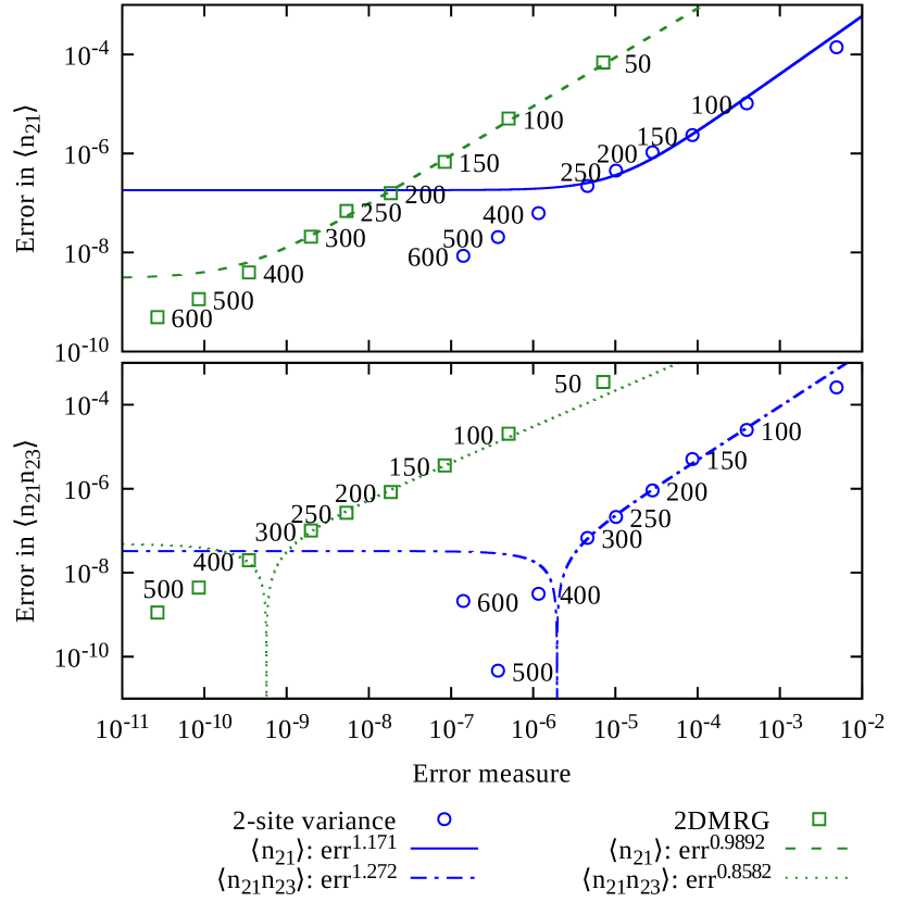
The variance of $\hat{H}$ with respect to our current state $|\psi\rangle$ is hence the norm squared of the residuum $|\phi\rangle=\hat{H}|\psi\rangle-E|\psi\rangle$. It is an extremely useful tool to check the convergence of DMRG and – contrary to the 2DMRG truncation error – can not just diagnose insufficient bond dimensions but also other convergence problems. When extrapolating the energy $E$ in the variance $v$, we typically expect a linear behavior, i.e. $E(v)=a\cdot v+E_{0}$. For other observables, the exponent may be different from one depending on the system at hand, the observable and how well either 1DMRG or 2DMRG can optimize this observable. In Sec. V.3, we provide one example to show the different range of exponents potentially encountered in such extrapolations.

Unfortunately, calculation of $\langle\hat{H}^{2}\rangle$ is computationally relatively expensive. A naive evaluation scales as $O(m^{3}dw^{2}+m^{2}d^{2}w^{3})$. First evaluating $\hat{H}^{2}$ and applying a MPO compression schemeFröwis et al. (2010); Hubig et al. (2017) allows us to reduce this to the calculation of the expectation value of a larger MPO with bond dimension $w^{\prime}$. In most cases, $w^{\prime}\approx 2w$. While this is unproblematic for simple one-dimensional systems with nearest-neighbor interactions, more complicated systems (e.g. from embedded problems, cylindrical systems or direct application of DMRG to quantum chemistry models) also result in much larger MPO bond dimensions $w$ which make evaluation of the variance unfeasible or at least much more costly than the initial DMRG calculation which lead to the state $|\psi\rangle$. In particular, there is a region (roughly $m\approx 10000$ and $w\approx 50$) where DMRG calculations and evaluation of simple observables are possible, but evaluating $\langle\psi|\hat{H}^{2}|\psi\rangle$ or $\hat{H}|\psi\rangle$ is not.

IV Proposed new error measure: 2-site variance

Figure 3: Top: Individual term of the projector $\hat{P}_{1}$, to be summed over all sites. Bottom: Individual term of the projector $\hat{P}_{2}$, to be summed over all pairs of neighboring sites. Tensors $F_{i}$ and $G_{i}$ are drawn as non-filled triangles.

The complete Hilbert space $\mathcal{H}$ may not only be decomposed into a product of local Hilbert spaces, but, given a MPS $|\psi\rangle$, also into a direct sum of orthogonal spaces

$$\mathcal{H}=\bigoplus_{l=0}^{L}\mathcal{W}_{l}$$ (18)

where $\mathcal{W}_{0}$ is the one-dimensional space of states parallel to $|\psi\rangle$ and $\mathcal{W}_{l}$ are the spaces of variations of $l$ continuous sites orthogonal to all $\mathcal{W}_{k<l}$. $\mathcal{W}_{L}$ could potentially span the entirety of $\mathcal{H}$ due to the completeness of matrix-product states, with only the subspaces already contained in $\mathcal{W}_{k<L}$ removed from it. Depending on the state $|\psi\rangle$, the partition of $\mathcal{H}$ into $\mathcal{W}_{l}$ changes.

Specifically, $\mathcal{W}_{1}$ is spanned by the states

$$|\phi^{(1)}_{i}(V)\rangle=\sum_{\boldsymbol{\sigma}}\cdots A_{i-1}\cdot F_{i}\cdot V_{i}\cdot B_{i+1}\cdots|\boldsymbol{\sigma}\rangle$$

$$\quad\forall i\in[1,L]\quad\forall V_{i}\in\mathbb{C}^{m_{i}^{\prime}}_{m_{i}}$$ (19)

and similarly $\mathcal{W}_{2}$ by the states

$$|\phi^{(2)}_{i,i+1}(W)\rangle=\sum_{\boldsymbol{\sigma}}\cdots A_{i-1}\cdot F_{i}\cdot W_{i}\cdot G_{i+1}\cdot B_{i+2}\cdots|\boldsymbol{\sigma}\rangle$$

$$\quad\forall i\in[1,L-1]\quad\forall W_{i}\in\mathbb{C}^{m_{i}^{\prime}}_{m^{\prime}_{i}}\quad.$$ (20)

The tensors $F_{i}$ and $G_{i}$ have the properties as defined in Eqs. (12) through (15). The projector $\hat{P}_{1}$ into the space $\mathcal{W}_{1}$ is given by $\sum_{i}|\phi^{(1)}_{i}\rangle\langle\phi^{(1)}_{i}|$ with the matrix $V_{i}$ left off and the left-hand side legs of $B_{i+1}$ and $B^{\dagger}_{i+1}$ as well as the right-hand side legs of $F_{i}$ and $F^{\dagger}_{i}$ connected. Similarly, the projector $\hat{P}_{2}$ into the space $\mathcal{W}_{2}$ is given by $\sum_{i}|\phi^{(2)}_{i,i+1}\rangle\langle\phi^{(2)}_{i,i+1}|$ connected in the same way. Individual terms of these two projectors are illustrated in Fig. 3. The projector $\hat{P}_{0}$ for $\mathcal{W}_{0}$ is simply $|\psi\rangle\langle\psi|$.

If we now consider the full variance $\langle\psi|(\hat{H}-E)(\hat{H}-E)|\psi\rangle$ of a normalized state $|\psi\rangle$, we may insert an identity $\mathbf{1}=\sum_{l=0}^{L}\hat{P}_{l}$:

$$\langle\psi|(\hat{H}-E)(\hat{H}-E)|\psi\rangle$$ (21)

$$= \langle\psi|(\hat{H}-E)\left[\sum_{l=0}^{L}\hat{P}_{l}\right](\hat{H}-E)|\psi\rangle$$ (22)

$$\approx \langle\psi|(\hat{H}-E)\left(\hat{P}_{0}+\hat{P}_{1}+\hat{P}_{2}\right)(\hat{H}-E)|\psi\rangle$$ (23)

$$= \langle\psi|\hat{H}\hat{P}_{1}\hat{H}|\psi\rangle+\langle\psi|\hat{H}\hat{P}_{2}\hat{H}|\psi\rangle\quad,$$ (24)

where all other terms of the form $\langle\psi|\hat{H}\hat{P}_{1,2}E|\psi\rangle$ are identically zero due to the orthogonality of $\hat{P}_{1,2}|\phi\rangle$ and $|\psi\rangle$ for all $|\phi\rangle$ and $\langle\psi|(\hat{H}-E)\hat{P}_{0}(\hat{H}-E)|\psi\rangle\equiv 0$ as well.

Figure 4: Top: One of the $L$ one-site contributions to the variance. Bottom: One of the $L-1$ two-site contributions to the variance. Temporary tensors $X_{i}$ and $Y_{i+1}$ (excluding $F_{i}$ and $G_{i+1}$), to be calculated during the evaluation of $L_{i}$ an $R_{i+1}$, are marked. Tensors $F_{i}$ and $G_{i}$ are drawn as non-filled triangles.

There are a total of $2L-1$ terms in Eq. (24), all of which can be written as squared Frobenius norms of rank-2 tensors (cf. Fig. 4).

Note that, if the Hamiltonian is composed of nearest-neighbor interactions only, the approximation in Eq. (23) becomes an equality. In this case, the Hamiltonian is a sum of nearest-neighbor terms $\hat{h}_{i,i+1}$. Applying such a term to the state $|\psi\rangle$ only has to change its MPS tensors on sites $i$ and $i+1$ (to see this, consider $\hat{h}_{i,i+1}$ as a two-site MPO gate). $\hat{h}_{i,i+1}|\psi\rangle$ is hence contained in $\mathrm{span}\left(|\psi\rangle,|\phi^{(1)}_{i}(V)\rangle,|\phi^{(2)}_{i,i+1}(W)\rangle\right)$ for suitably-chosen $V,W$ and hence in $\mathcal{W}_{0}\oplus\mathcal{W}_{1}\oplus\mathcal{W}_{2}$.

Equally, if we were to include also $\hat{P}_{3}$, we could calculate the variance of a three-site operator exactly (albeit at $d$-times higher computational effort).

In such cases, the 2-site variance proposed here is actually a remarkably stable and numerically precise way to evaluate the variance: the large terms of order $E^{2}$ are removed exactly, which would otherwise incur a loss of approximately $\mathrm{log}_{10}(E^{2})$ digits of precision when evaluating $\langle H^{2}\rangle-\langle E\rangle^{2}$ directly. We also avoid the alternative subtraction in $\langle(\hat{H}-E)^{2}\rangle$ which still incurs losing approximately $\mathrm{log}_{10}(|E|)$ digits. Instead, only positive, small terms of order $\langle(H-E)^{2}\rangle/L$ are added together. We are left with the unavoidable loss of precision due to repeated matrix-matrix products of one or two digits relative to the machine epsilon. This effect is demonstrated in Fig. 5, where four possible approaches to evaluate the variance in a $S=1$, $L=200$ Heisenberg chain with open boundary conditions are compared. The 2-site variance is one of the two most precise methods and also the fastest method: for example, the last data points at $m=340$ in Fig. 5 took $26\text{\,}\mathrm{s}$ for the 2-site variance, $41\text{\,}\mathrm{s}$ for $\langle\hat{H}^{2}\rangle-\langle E\rangle^{2}$, $41\text{\,}\mathrm{s}$ for $\langle(\hat{H}-E)^{2}\rangle$ and $436\text{\,}\mathrm{s}$ for $\left|\left|\hat{H}|\psi\rangle-E|\psi\rangle\right|\right|^{2}$ on a two-core Intel i5-6200U CPU. This system is the best-case scenario for calculation of the full variance due to the small original bond dimension of $\hat{H}$ with just $w=5$. On more complicated systems, the relative advantage of the 2-site variance will be more pronounced.

Figure 5: (Color online) Comparison of different ways to evaluate the variance $\langle(\hat{H}-E)^{2}\rangle$ of a $L=200$ sites $S=1$ Heisenberg model at different $\mathrm{SU}(2)_{\mathrm{Spin}}$-invariant bond dimensions. The error in energy relative to $E_{0}\approx-279.088490029140\pm 2\times 10^{-12}$ is given in gray for comparison and shown to saturate numerical precision around $m\approx 180$. Of the three alternatives to the 2-site variance, only $||\hat{H}|\psi\rangle-E|\psi\rangle||^{2}$ is equally precise but requires a full MPO-MPS product and an MPS-MPS addition, making it much more costly.

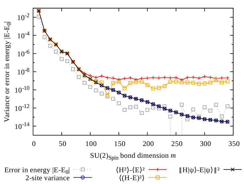
Depending on the number of cores available, different procedures yield the fastest wall-clock time and least memory/temporary disk space usage when evaluating the 2-site variance:

If only a single core is available, it is reasonable to first left-normalize $|\psi\rangle$, evaluate $L_{i}$ and store $X_{i}\cdot F_{i}^{\dagger}$ (cf. Fig. 4, $X_{i}=L_{i-1}\cdot W_{i}\cdot A_{i}$) for all sites. The $L_{i}$ do not have to be stored. Then, sweeping right-to-left, one first right-normalizes $M_{i+1}$ into $B_{i+1}$ and $T$. $B_{i+1}$ is used to evaluate $Y^{\prime}_{i+1}=R_{i+2}\cdot W_{i+1}\cdot B_{i+1}$ which is stored temporarily. $G^{\dagger}_{i+1}$ and $T$ are contracted into $Y^{\prime}_{i+1}$ and the result is then contracted with the left half to yield the rank-2 tensor depicted in Fig. 4, bottom panel. The squared Frobenius norm of this tensor is taken and added to the accumulator. One then evaluates $R_{i+1}$ by re-using $Y^{\prime}_{i+1}$, moves $T$ into the next site tensor to the left as well as into the contraction $X_{i}$ to yield $X^{\prime}_{i}$. $X^{\prime}_{i}$ is contracted with $R_{i+1}$ to give the tensor in Fig. 4, upper panel. Its squared Frobenius norm is again added to the accumulator and one moves to the next site.

If, on the other hand, many cores are available, it is reasonable to parallelize the most expensive part, namely the calculation of $F_{i}$ and $G_{i}$ as well as the products leading to the tensors in Fig. 4. This can be done by first evaluating $X_{i}$ and $Y_{i}$ as well as $R_{i}$ on all sites by two independent processes acting on two left- and right-normalized copies of $|\psi\rangle$. Once these contractions are available and e.g. stored temporarily on disk, one may start $2L-1$ processes, each evaluating one of the $2L-1$ individual terms.

The costs of this procedure are distributed as follows: Left- and right-normalization as well as calculation of $X_{i}$, $Y_{i}$, $R_{i}$ and the (temporary) $L_{i}$ all scale as $O(m^{3}dw)$ and are roughly twice as expensive as calculating a single expectation value $\langle\psi|\hat{H}|\psi\rangle$, but can be parallelized two-fold. The generation of $F_{i}$ and $G_{i}$ scales as $O(m^{3}d(d-1))$ but can be parallelized $2L-1$-fold. Contractions $X_{i}\cdot F^{\dagger}_{i}$ and $Y_{i+1}\cdot G_{i+1}^{\dagger}$ cost $O(m^{3}d(d-1)w)$ each, the contraction $X_{i}F_{i}^{\dagger}\cdot Y_{i+1}G_{i+1}^{\dagger}$ costs $O(m^{3}(d-1)^{2}w)$, but these can also be parallelized perfectly.

As such, the serial part of the calculation takes wall-clock time comparable to a single expectation value calculation. The following, $2L-1$-fold parallelized part scales worse in the local physical dimension than the pure 1DMRG, but already better than 2DMRG. Its primary components, the two full QRs to calculate $F_{i}$ and $G_{i}$, are also much cheaper than the SVD of the two-site tensor in 2DMRG both asymptotically (by a factor of $d$) and in practical calculations.

V Examples

The first two examples are intended to show that the variance itself is a valid extrapolation tool and as useful as the 2DMRG truncation error. This is done at the example of nearest-neighbor interaction chains of Heisenberg spins and Hubbard electrons. Next, we show at the example of long-range Coulomb-like interactions that even if the full variance and two-site variance do not coincide due to long-range interactions, both yield comparable results. Finally, we consider the Hubbard model on a cylinder where it is impractical to calculate the full variance but extrapolation in the two-site variance is as useful as extrapolation in the 2DMRG truncation error.

V.1 Introductory remarks

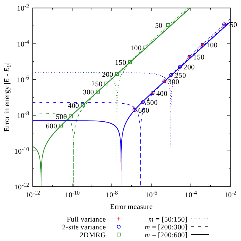
In the following Figs. 6 through 11, we show stages of the calculations always as points with select bond dimensions indicated by nearby numbers. The y-axis position of each point is given by the observable expectation value (in Figs. 10 and 11) or the error compared to the true ground state expectation value (in Figs. 6-9) at that particular stage. The x-axis position is given by the error measurement used, i.e. either the 2DMRG truncation error (always in green), the full variance (in red where available) or the 2-site variance (always in blue) as observed at this stage. Errors in energy and error measures smaller than the plot range (typically $10^{-14}$) were clipped to that value for illustrative purposes. The error measures were likewise scaled by constant factors to fit into the same plot (this does not affect the extrapolation).

For the energies plotted in Figs. 6, 7 and 9-11, linear extrapolations towards zero error were attempted over several intervals, each containing a certain number of data points obtained from the calculation. In the plots, the least to most accurate extrapolations are always shown as dotted, dashed, dash-dotted and solid lines respectively. In Fig. 8, the exponent was also selected as a fit parameter and only one extrapolation performed per data set.

Ideally, extrapolations over intervals with smaller bond dimensions are validated by calculations at higher bond dimensions: In Fig. 6, we would like the data points at bond dimension 160 to lie on the line extrapolated from bond dimensions $[2,\ldots,m^{\prime}\ll 160]$. We can hence also judge the quality of an extrapolation by observing its change when including additional data points.

Furthermore, a correct extrapolation in Figs. 6 through 9 would result in a y-intercept of zero, indicating that the extrapolation produced the exact (error-free) value. Deviations from this ideal case (i.e., non-zero y-intercepts) result in saturated constant extrapolations at small error values. If the extrapolated value is smaller than the true ground-state value, the resulting zero crossing displays as a narrow dip in the extrapolation curve.

In Fig. 10 and 11, no exact reference values are available, making the log-log plot impossible. We hence show in total three different ranges of the calculation with linear scales on both axes.

For the 2DMRG calculations, the energy is measured during the calculation and prior to each local truncation, resulting in a larger effective bond dimension for 2DMRG and a slightly lower energy. This would also be done in actual calculations specifically to exploit this locally larger dimension for more accurate measurements. We hence have not eliminated this advantage by bringing the 2DMRG state into canonical form before evaluating its energy. For the variance measures, 1DMRG with subspace expansion (DMRG3SHubig et al. (2015)) is used and the energy is evaluated as the expectation value of the Hamiltonian with respect to the final MPS.

V.2 Heisenberg spin chain

As the first example, we wish to analyze the convergence behavior of a $L=30$ Heisenberg spin chain with open boundary conditions. Only the $\mathrm{U}(1)$ symmetry is implemented, but the Hamiltonian itself is rotationally invariant:

$$\hat{H}=\sum_{i=1}^{29}\sum_{a=x,y,z}\hat{s}^{a}_{i}\hat{s}^{a}_{i+1}\quad.$$ (25)

30 sweeps each are run with bond dimensions $m=2,4,6,8,\ldots,160$. For the reference value of the ground-state energy $E_{0}=-13.1113557586032048\pm 5\times 10^{-14}$, a calculation with $m=500$ is run. This ground state can be truncated with a truncation error less than $10^{-16}$ to $m=160$, giving the upper bound in the above series.

In Fig. 6 we plot the energy differences to the ground state over the three error measures. Three linear extrapolations in the ranges $m\in[2,12]$, $m\in[14,36]$ and $m\in[14,60]$ are done. The first range represents the case of only a bad, low-precision calculation being available, the other ranges showcase the increased precision attainable and – as usually done – exclude the lowest-precision data points.

Figure 6: (Color online) Energy differences from the true ground state and error measures (cf. Sec. V.1) for the $L=30$ Heisenberg chain. Both the 2DMRG truncation error and the error measure based on either the full or 2-site variance result as expected in essentially straight lines of slope $1$ in the log-log plot. The full and 2-site variance overlap completely due to the short-range Hamiltonian.

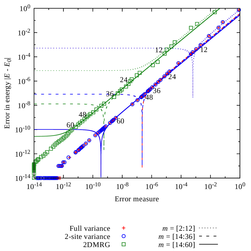
The first extrapolation provides a much improved extrapolated ground-state energy estimate with 2DMRG as compared to the two methods based on 1DMRG. This is likely due to the increased effective bond dimension in 2DMRG. In later extrapolations, all extrapolated ground-state energies are within an order of magnitude.

To summarize the Heisenberg model, we find mostly identical behavior between an extrapolation in the variance and and the 2DMRG truncation error. The latter sometimes provides better data, likely due to the larger effective bond dimension. Generally, extrapolation can lower the energy difference $|E-E_{0}|$ from the true ground state by an order of magnitude.

V.3 Hubbard chain

Figure 7: (Color online) Energy differences from the true ground state and error measures (cf. Sec. V.1) for the $L=50$ Hubbard chain. Three extrapolation regions were selected and the three error measures mostly lead to equally valid extrapolations towards zero error. The full and 2-site variance overlap completely due to the short-range Hamiltonian. The error in the energy is reduced by approximately an order of magnitude via the extrapolation.

Figure 8: (Color online) Exemplary behavior of $\langle\hat{n}_{21}\rangle$ (top) and $\langle\hat{n}_{21}\hat{n}_{23}\rangle$ (bottom) in the Hubbard chain. Fits of the form $a\cdot\mathrm{err}^{b}+c$ in the interval $m\in[100,300]$ are shown with the exponent $b$ ranging from $0.85$ to $1.27$ in these cases. Since the 2-site variance correctly calculates the full variance in this nearest-neighbor case, it is not shown in the figure.

As a second system, we consider the Fermi-Hubbard model on a chain of $L=50$ sites with open boundary conditions. The Hubbard-$U$ parameter is set to $8$, $t=1$:

$$\hat{H}= -\sum_{i=1}^{49}\left(\hat{c}^{\dagger}_{i}\cdot\hat{c}_{i+1}+\mathrm{h.c.}\right)+\frac{8}{2}\sum_{i=1}^{50}\left(\hat{n}_{i}^{2}-\hat{n}_{i}\right)\quad.$$ (26)

Both the $\mathrm{U}(1)_{N}$ and $\mathrm{SU}(2)_{S}$ symmetries are implemented (leading to two-component spinors $\hat{c}$ and $\hat{c}^{\dagger}$). We select the sector $N=40,S=0$ for the ground-state search. The reference value for the ground-state energy $E_{0}=30.4096693772556\pm 3\times 10^{-13}$ is provided by a calculation at $m=2000$, the test calculations are run at $m=50,100,150,200,250,300,400,500$ and $600$ .

Extrapolations over the regions $m\in[50,150]$, $m\in[200,300]$ and $m\in[200,600]$ show that at small accuracies, all extrapolations have roughly equal errors. At higher accuracies, the 2DMRG again benefits from its larger effective bond dimension. As expected, the full variance and two-site variance approximation coincide again, as this Hamiltonian also only has nearest-neighbor interactions. All extrapolations lead to equally valid results and lower the error in energy by approximately an order of magnitude.

In addition to the error in energy, we also consider the observables $\langle\hat{n}_{21}\hat{n}_{23}\rangle$ and $\langle\hat{n}_{21}\rangle$, again compared to a reference value evaluated at $m=2000$. The following noteworthy observations can be made: first, $\langle\hat{n}_{21}\hat{n}_{23}\rangle$ seems to be accurate down to approx. $10^{-9}$ with the error saturating there. Second, in the extrapolation of this observable, both 2DMRG and the 2-site variance only lower the measured error by approximately a factor of two. Third, when evaluating $\langle\hat{n}_{21}\rangle$, the 2DMRG results are consistently more accurate than those from 1DMRG, possibly due to the two-site optimization applying better to this observable. Fourth, the optimal coefficients $b$ in a fit of the form $a\cdot\mathrm{err}^{b}+c$ range from $0.85$ to $1.27$ in these examples. Overall, while extrapolation of these observables is more difficult, it is still possible to obtain improved estimates for the true value at the ground state.

V.4 Long-range Coulomb interactions

Figure 9: (Color online) Energy differences from the true ground state and error measures (cf. Sec. V.1) for the model with long-range Couloumb-like interactions. While the full variance and two-site approximation thereof differ, both lead to comparable extrapolations which in turn are comparable to those based on 2DMRG.

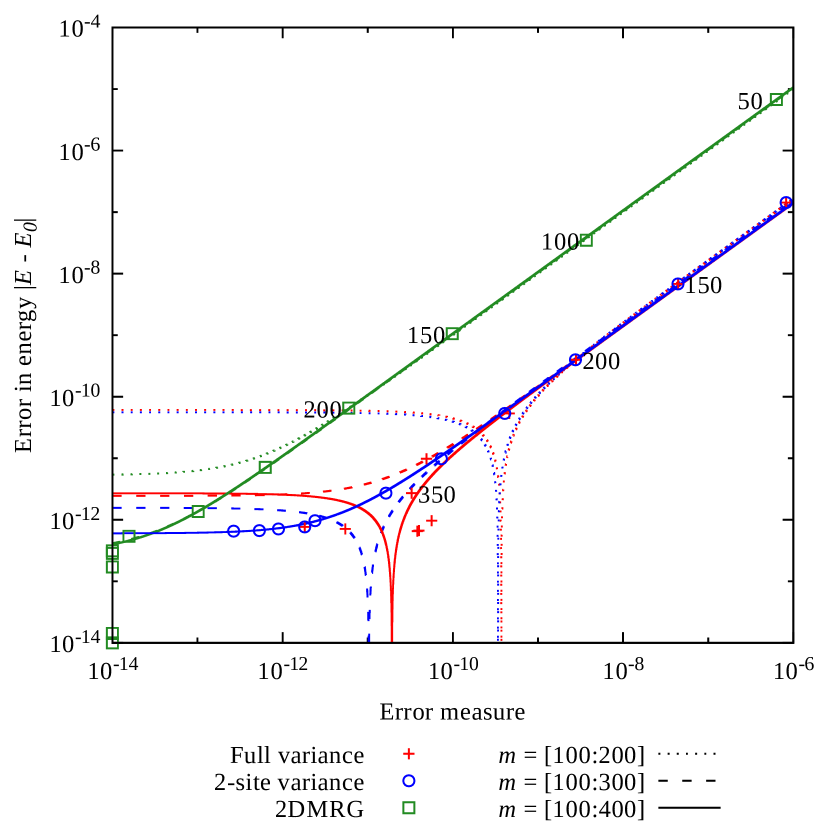
As an example of long-range Hamiltonians which will lead to a difference between the full variance and the two-site approximation of the variance, we selected an electronic model with Coulomb-like long-range interactions. The Hamiltonian, again implementing both the $\mathrm{U}(1)_{N}$ and $\mathrm{SU}(2)_{S}$ symmetries, is given by

$$\hat{H}=\sum_{i=1}^{19}\hat{c}_{i}^{\dagger}\cdot c_{i+1}+\mathrm{h.c.}+\sum_{i=1}^{20}\sum_{j=i}^{20}\frac{1}{1+|i-j|}\hat{n}_{i}\hat{n}_{j}\quad.$$ (27)

$N=30$ electrons with total spin $S=0$ were placed in the system. Due to the strong repulsion and relatively small system size, solutions exhaust numerical accuracy around $m\approx 400$ with the reference value $E_{0}=111.43149155591837\pm 5\times 10^{-12}$ evaluated at $m=600$. Test calculations are run at $m=50,100,150,\ldots,500$ and extrapolations are for $m\in[100,200]$, $m\in[100,300]$ and $m\in[100,400]$.

Apart from a minor advantage enjoyed by 2DMRG due to the momentarily larger bond dimensions, the results largely coincide between 2DMRG, the full variance and the 2-site variance. In particular, the extrapolations based on the full variance and the two-site variance mostly coincide very well and lower the error in the energy again by approximately an order of magnitude.

V.5 Hubbard cylinder

Figure 10: (Color online) Extrapolation of energies towards zero error (cf. Sec. V.1) in the Hubbard model on a cylinder. Main plot: Values used for extrapolation at $m\geq 2000$. Inset: Measured energies and errors at all bond dimensions with the first extrapolation over $m\in[2000,4000]$ for comparison.

Figure 11: (Color online) Zoomed version of Fig. 10. The consecutive corrections of the ground-state energy estimates based on more and more data are clearly visible. Again, extrapolated energies increase with bond dimension since extrapolated energies, as opposed to calculated energies, do not obey a variational principle.

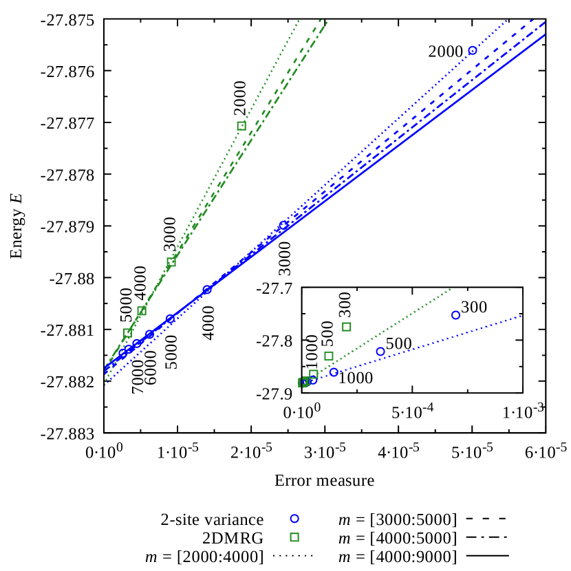
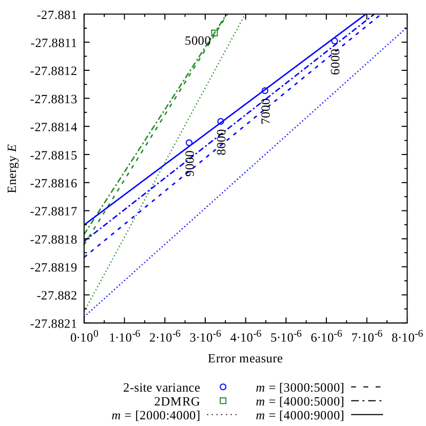
As the final example, we will attempt to calculate the ground-state energy of the Hubbard model on a cylinder of size $10\times 4$. $U(1)_{N}$ particle number conservation, $\mathrm{SU}(2)_{S}$ total spin symmetry and $\mathbb{Z}_{4,k}$ quasi-momentum conservation on the cylinder were implemented. The Hubbard-$U$ parameter is set to $8$, $t=1$:

$$\hat{H}= -\sum_{x=1}^{10}\sum_{\alpha=1}^{4}2\cos\left(2\pi\frac{\alpha}{4}\right)\hat{c}^{\dagger}_{x,\alpha}\cdot\hat{c}_{x,\alpha}$$

$$-\sum_{x=1}^{9}\sum_{\alpha=1}^{4}\left(\hat{c}^{\dagger}_{x,\alpha}\cdot\hat{c}_{x+1,\alpha}+\mathrm{h.c.}\right)$$

$$+\frac{8}{2}\sum_{x=1}^{10}\sum_{\alpha=1}^{4}\left[\sum_{\beta\gamma=1}^{4}\frac{1}{4}\hat{c}^{\dagger}_{x,\alpha}\cdot\hat{c}_{x,\beta}\times\hat{c}^{\dagger}_{x,\gamma}\cdot\hat{c}_{x,\alpha-\beta+\gamma}\right]$$

$$-\frac{8}{2}\sum_{x=1}^{10}\sum_{\alpha=1}^{4}\hat{c}^{\dagger}_{x,\alpha}\cdot\hat{c}_{x,\alpha}\quad.$$ (28)

$\hat{c}^{(\dagger)}_{x,\alpha}$ is the two-component spinor annihilating (creating) an electron on ring $x$ with momentum $\alpha$. The two last lines implement the real-space on-site interaction which, in momentum space along each ring, becomes long-ranged. $N=36$ electrons with total spin $S=0$ and momentum $k=0$ were placed in the system.

Table 1: Resulting energy expectation values at $m=5000$ and $m=9000$ and extrapolated ground-state energy estimates for the Hubbard model on a cylinder.

$m$	1DMRG & 2-site var.	2DMRG
$5000$	$-27.8807953$	$-27.8810672$
$9000$	$-27.8814580$	–
$[2000,4000]$	$-27.8820779$	$-27.8820598$
$[3000,5000]$	$-27.8818661$	$-27.8818215$
$[4000,5000]$	$-27.8818090$	$-27.8817841$
$[4000,9000]$	$-27.8817508$	–

Due to the complicated system, no exact reference calculation was possible. 2DMRG was run at bond dimension $m=300,500,1000,2000,3000,4000$ and $5000$. With 1DMRG, increasing $m$ further to $m=6000,7000,8000$ and $m=9000$ was possible due to lower computational effort and less memory usage. The $m=9000$ $\mathrm{SU}(2)$-invariant states correspond to roughly $24^{\prime}000$ states if only symmetries without inner multiplicity were used. Evaluating the full variance was not possible due to the large MPO bond dimension.

In the extrapolations, the initial data at $m<1000$ was discarded and extrapolations over $m\in[2000,4000]$, $m\in[3000,5000]$ and $m\in[4000,5000]$ were done for both 2DMRG and 1DMRG data as well as $m\in[4000,9000]$ for 1DMRG data. Both extrapolations in 2DMRG truncation error and the two-site variance initially underestimated the ground-state energy with later extrapolations correcting the estimate slightly upwards. Extrapolations at $m\in[2000,4000]$ and $m\in[3000,5000]$ give nearly the same results between the 2-site variance and 2DMRG.

The 2-site variance further corrects the estimate upwards for $m\in[4000,5000]$ and $m\in[4000,9000]$ resulting in a highest-precision estimate for the ground-state energy of $-27.8817508$ compared to the highest-precision 2DMRG estimate of $-27.8817841$ (cf. Tab. 1).

VI Conclusions

We have shown that the variance itself as well as its two-site approximation allow for a reliable extrapolation of observables to the ground state from a series of small-$m$ states. Measuring the two-site approximation of the variance is considerably cheaper than evaluating the full variance and leads to valid extrapolations comparable in quality to those resulting from 2DMRG. It hence allows the use of 1DMRG with its significant speed-up and reduced memory usage over the traditional 2DMRG.

All extrapolations encountered here lower the error in energy by approximately one order of magnitude from the most precise data point available, consistent with previous observations.White (2005) We must stress, however, that the variational property of DMRG is lost if we use any sort of extrapolation.