Randomized exponential integrators for modulated nonlinear Schrödinger equations

Abstract.

We consider the nonlinear Schrödinger equation with dispersion modulated by a (formal) derivative of a time-dependent function with fractional Sobolev regularity of class $W^{\alpha,2}$ for some $\alpha\in(0,1)$. Due to the loss of smoothness in the problem classical numerical methods face severe order reduction. In this work, we develop and analyze a new randomized exponential integrator based on a stratified Monte Carlo approximation. The new discretization technique averages the high oscillations in the solution allowing for improved convergence rates of order $\alpha+1/2$. In addition, the new approach allows us to treat a far more general class of modulations than the available literature. Numerical results underline our theoretical findings and show the favorable error behavior of our new scheme compared to classical methods.

1. Introduction

We study modulated nonlinear Schrödinger equations of the form

(1) $$i\partial_{t}u(t,x)+\Delta u(t,x)\partial_{t}g(t)=\left|u(t,x)\right|^{2}u(t,x),\quad u(0,x)=u_{0}(x),\quad(t,x)\in\mathbb{R}\times\mathbb{T}^{d},$$

where $g:\mathbb{R}\to\mathbb{R}$ is an arbitrary function of time with fractional Sobolev regularity of class $W^{\alpha,2}$ (see (5) for the definition) with $\alpha\in(0,1)$.

Classical semilinear Schrödinger equations with $g(t)=t$ are nowadays extensively studied numerically. In this context, splitting methods (where the right-hand side is split into the kinetic and nonlinear part, respectively) as well as exponential integrators (based on approximating Duhamel’s formula) contribute particularly attractive classes of integration schemes. For an extensive overview on splitting and exponential integration methods we refer to [17, 18, 19, 30], and for their rigorous convergence analysis in the context of semilinear Schrödinger equations we refer to [4, 6, 9, 12, 15, 16, 28] and the references therein.

In the last decades, the modulated Schrödinger equation (1) has gained a lot of attention in physics serving, e.g., as a model describing propagation of light waves in optical dispersion-managed fibers (see for instance [1, 7, 10, 11, 20, 21, 25, 32]). Numerically, however, only very little is known so far for this type of problem. The highly oscillatory nature of the problem makes the construction and analysis of numerical schemes for (1) particularly challenging in non-smooth regimes, where $g$ is of fractional Sobolev regularity of class $W^{\alpha,2}$ with exponent $\alpha\in(0,1)$. Due to the loss of smoothness in the system classical numerical schemes (e.g., splitting methods, exponential integrators, etc.) face severe order reduction. This is due to the fact that their rate of convergence heavily depends on the smoothness of $g$. To allow a reliable approximation classical numerical schemes are thus subject to severe step size restrictions which leads to large errors and huge computational costs in case of non-smooth modulations $g$. We refer to [13, 17] for an extensive overview on the numerical analysis of highly oscillatory problems, and in particular to [22, 23] and the references therein for the numerical analysis of semiclassical Schrödinger equations. Recently, the case of $g$ being a Brownian motion, a stochastic process that has in particular $\alpha$-Hölder continuous trajectories for every $\alpha\in(0,1/2)$, has gained a lot attention in numerical analysis. Various numerical schemes have been proposed reaching from Crank-Nicolson discretizations [3] over splitting schemes [29] up to exponential integrators [8]. A rigorous error analysis of these schemes could be established based on probabilistic arguments, i.e., stating the ‘rate of convergence with certain probability’ (see (3) below for the detailed convergence bound). Whereas the used probabilistic arguments are applicable to Brownian motion they do not allow for an extension to more general modulations $g$ nor for deterministic error bounds. Up to our knowledge, nothing is known in the numerical analysis literature so far for a general modulated dispersion $\partial_{t}g(t)\Delta$ and, in particular, deterministic (pathwise) error bounds are still lacking.

In this work we consider for the first time the general case where the modulation $g$ is of fractional Sobolev regularity of class $W^{\alpha,2}$ in time and develop a new randomized exponential integration scheme for the modulated Schrödinger equation (1) in this general setting. For technical reasons, we also require that $g$ belongs to the Hölder space $C^{\varepsilon}$ for an arbitrarily small $\varepsilon\in(0,1)$. This allows us to prove the a priori boundedness of the numerical solution in the classical Sobolev space $H^{\sigma}$ (cf. [28]). Note that if $\alpha>1/2$ then according to the Sobolev embedding there exists $\varepsilon\in(0,1)$ such that $W^{\alpha,2}\subset C^{\varepsilon}$, so the additional assumption does not pose any further restriction.

Our new technique allows us to average the high oscillations in the solution and gain $1/2$ in the convergence rate. More precisely, we can firstly establish improved pathwise convergence rates of order $\alpha+1/2$ for the new scheme (see (2) below for the precise error estimate). In contrast, classical schemes require much stronger smoothness assumptions as they rely on the Hölder continuity of $g$. Even if $g$ is $\alpha$-Hölder continuous (and not only in $W^{\alpha,2}$) classical schemes face severe order reduction down to order $\alpha$ due to the loss of smoothness in the system. These theoretical findings are underlined by numerical experiments: while the error of classical schemes oscillates widely, reaching large errors, our proposed randomized exponential integrator allows us to average these oscillations maintaining its convergence rate with much smaller and reliable errors, see Section 4.

For completeness, note that randomized numerical schemes in various settings have already appeared in the literature, in particular in the context of ordinary differential equations and recently also in case of uncertainty quantifications [2] . Let us particularly mention [14, 24, 26, 27] which inspired our research and where further references can be found. However, to the best of our knowledge such a method was not yet applied in the context of dispersive equations such as (1). In [7], the modulated Schrödinger equation of type (1) has been studied from the analytical point of view. Thereby an Euler-like procedure was used to prove existence and construct solutions under certain regularity assumption on $g$. However, numerical analysis was not the objective of this work.

New approach in a nutshell. In the present paper we put forward an exponential integrator for (1) based on a stratified Monte Carlo approximation. More precisely, we consider the mild formulation of (1) and approximate the convolution integral appearing on the right hand side by means of a randomized Riemann sum. The key idea is to choose the randomization in such a way, that the associated error is a (discrete time) martingale, which permits to apply the so-called Burkholder-Davis-Gundy inequality (see Theorem 3.5). Remarkably, this allows to gain half in the convergence rate in expectation. More precisely, splitting the time interval $[0,T]$ into an equidistant partition $t_{0},\ldots,t_{N}$ with the mesh size $\tau=\frac{T}{N}$, for some $N\in\mathbb{N}$, we establish the following bound for the difference of the exact solution $u$ at time $t_{n}$ and the numerical solution $u^{n}$ valid for initial conditions in $H^{\sigma+2}$ with $\sigma>d/2$ (see Theorem 3.1 for details):

(2) $$\left(\mathbb{E}_{\xi}\max_{n=0,\dots,N}\|u(t_{n})-u^{n}\|_{H^{\sigma}}^{2}\right)^{1/2}\leq c\tau^{\min\{1,{\alpha+\frac{1}{2}}\}},$$

where $\mathbb{E}_{\xi}$ is the expected value associated to the randomization of the numerical scheme and $\alpha$ is the exponent of fractional Sobolev regularity of $g$. Classical numerical schemes are in contrast restricted to the Hölder continuity, see also Remark 3.2 below.

Comparison with previous results. We stress that the expectation above is taken only with respect to the randomization of the scheme, whereas the modulation $g$ is deterministic. In other words, in the case of a random modulation, such as the Brownian motion treated in [3, 8], our result provides pathwise error estimates leading to a pathwise convergence analysis. In addition, it applies to a wide range of possible modulations, deterministic or random, and in particular to any other stochastic process with trajectories of fractional Sobolev regularity, overcoming the limitations of [7].

Note that in [3] a semi-discrete Crank-Nicolson scheme is analyzed. The strong order of convergence in probability in $H^{\sigma}$, $\sigma>d/2$, is equal to one for initial conditions in $H^{\sigma}$ for this scheme. In [8] an explicit exponential integrator is proposed and it is shown that it is mean-square order 1 in $H^{\sigma}$ for initial conditions in $H^{\sigma+4}$.

In both works [3, 8], a stochastic approach was used and it was only possible to obtain the order of convergence $1$ in probability which reads as

(3) $$\lim_{C\to\infty}\mathbb{P}_{W}\big{(}\|u(t_{n})-u^{n}\|_{\sigma}>C\tau\big{)}=0,$$

for all $n=0,\dots,N$ uniformly with respect to $\tau$. Here we write $\mathbb{P}_{W}$ to denote the probability measure on the probability space where the Brownian motion $g=W$ is defined (in contrast to the notation $\mathbb{E}_{\xi}$ above which only concerns the artificial randomness introduced in our scheme). It was conjectured in [3] that a stronger result should hold, namely,

$$\lim_{C\to\infty}\mathbb{P}_{W}\Big{(}\max_{n=0,\dots,N}\|u(t_{n})-u^{n}\|_{\sigma}>C\tau\Big{)}=0,$$

uniformly with respect to $\tau$. However, the proof would require very tedious computations which were not presented. Our approach allows to overcome this challenge and the convergence analysis is rather elegant and simple. See Remark 3.7 below.

Organization of the paper. Our exponential integrator is derived in Section 2. In Section 3 we carry out a rigorous error analysis for the new scheme. In Section 4 we present numerical experiments for $g$ belonging to $W^{\alpha,2}$ for various $\alpha\in(0,1)$.

For practical implementation issues we impose periodic boundary conditions, i.e, $x\in\mathbb{T}^{d}=[0,2\pi]^{d}$, $d\in\mathbb{N}$. For notational simplicity we work with cubic nonlinearities. However, the generalization to polynomial nonlinearities $f(u)=|u|^{2p}u$ is straightforward.

Notation. In the following let $\sigma>d/2$. We denote by $\|\cdot\|_{\sigma}$ the standard $H^{\sigma}=H^{\sigma}(\mathbb{T}^{d})$ Sobolev norm, that is, if $f\in H^{\sigma}$ such that $f(x)=\sum_{k\in\mathbb{Z}^{d}}\hat{f}_{k}\mathrm{e}^{ik\cdot x}$, $x\in\mathbb{T}^{d}$, then

$$\|f\|_{\sigma}=\left(\sum_{k\in\mathbb{Z}^{d}}(1+|k|^{2})^{\sigma}|\hat{f}_{k}|^{2}\right)^{1/2}.$$

In particular, we exploit the well-known bilinear estimate

(4) $$\|f_{1}f_{2}\|_{\sigma}\leq c_{\sigma}\|f_{1}\|_{\sigma}\|f_{2}\|_{\sigma}$$

which holds for some constant $c_{\sigma}>0$ and every $f_{1},f_{2}\in H^{\sigma}$. The space of $\varepsilon$-Hölder continuous functions for $\varepsilon\in(0,1)$ is denoted by $C^{\varepsilon}$, whereas $C([0,T];H^{\sigma})$ denotes the space of continuous functions with values in $H^{\sigma}$. Furthermore, for $\alpha\in(0,1)$ we let $W^{\alpha,2}$ denote the fractional Sobolev space on $(0,T)$ (also called the Sobolev-Slobodeckij space) given by the norm

(5) $$\|g\|_{W^{\alpha,2}}=\left(\int_{0}^{T}|g(t)|^{2}\mathrm{d}t+\int_{0}^{T}\int_{0}^{T}\frac{|g(r)-g(s)|^{2}}{|r-s|^{2\alpha+1}}\mathrm{d}r\mathrm{d}s\right)^{\frac{1}{2}}.$$

For two quantities $a,b$, we use the notation $a\lesssim b$ to say that there exists a constant $c>0$ such that $a\leq cb$. This proportionality constant will typically depend on data of the problem and/or certain norms of the exact solution, which we always specify below. However, it will always be independent of the step size $\tau$ and $N$.

2. Derivation of the numerical scheme

It is possible to make sense of (1) using the associated mild formulation. To this end, let us set

$$S(t)=S^{g}(t)=e^{ig(t)\partial^{2}_{x}},\quad t\in\mathbb{R},$$

as well as

$$U(t,r)=S(t)S(r)^{-1}=e^{i[g(t)-g(r)]\partial^{2}_{x}}$$

such that in particular $U(t,0)=S(t)$. Note that due to the presence of the modulation $g$, the problem (1) is not time-homogeneous. Consequently, the linear part of (1) generates an evolution system given by the family of operators $U(t,r)$, $r,t\in\mathbb{R}$, which are (generally) not functions of the difference $t-r$ as it would be case in the classical setting, that is, $g(t)=t$. Intuitively, $U(t,r)$ describes the evolution of the linear part of (1) from time $r$ to time $t$. Note that since the modulation $g$ does not depend on the space variable $x$, the above operators are Fourier multipliers given by

$$\mathcal{F}[S(t)f](k)=e^{-ig(t)|k|^{2}}\hat{f}_{k},\qquad\mathcal{F}[U(t,r)f](k)=e^{-i[g(t)-g(r)]|k|^{2}}\hat{f}_{k}$$

for $f\in L^{2}$ such that $f(x)=\sum_{k\in\mathbb{Z}^{d}}\hat{f}_{k}\mathrm{e}^{ik\cdot x}$, $x\in\mathbb{T}^{d}$.

In the construction and analysis of our numerical scheme we will in particular exploit that the operators $U(t,r)$ and $S(t)$ are linear isometries in $H^{\sigma}$ for all $r,t\in\mathbb{R}$:

Lemma 2.1.

For all $f\in H^{\sigma}$ and $r,t\in\mathbb{R}$ we have that

(6) $$\|U(t,r)f\|_{\sigma}=\|f\|_{\sigma},\quad\|S(t)f\|_{\sigma}=\|f\|_{\sigma}.$$

Proof.

The assertion follows by the definition of the $H^{\sigma}$ norm together with the relation

$$\mathrm{e}^{ig(t)\partial_{x}^{2}}f(x)=\sum_{k\in\mathbb{Z}^{d}}\mathrm{e}^{-ig(t)|k|^{2}}\hat{f}_{k}\mathrm{e}^{ik\cdot x}$$

which holds for all $f\in L^{2}$ such that $f(x)=\sum_{k\in\mathbb{Z}^{d}}\hat{f}_{k}\mathrm{e}^{ik\cdot x}$, $x\in\mathbb{T}^{d}$. ∎

We point out that a well-posedness theory of (1) under the generality assumed in the present manuscript is very challenging and remains an open problem. Partial results were given in [7] covering for instance the case of a fractional Brownian motion $g$ and $d=1$. Our numerical study may help to better understand the properties of (1) for a general class of modulations $g$ with fractional Sobolev regularity and might set a starting point for further analytical investigations.

Our goal is to derive a numerical scheme for the mild solution of (1) given by Duhamel’s formula

(7) $$u(t)=U(t,0)u_{0}-i\int_{0}^{t}U(t,r)[|u(r)|^{2}u(r)]dr,\qquad t\in\mathbb{R}.$$

Using the flow property $U(t,\xi)=U(t,r)U(r,\xi)$ valid for all $\xi\leq r\leq t$, we deduce that it satisfies

$$u(t)=U(t,r)u(r)-i\int_{r}^{t}U(t,\xi)[|u(\xi)|^{2}u(\xi)]d\xi.$$

Let us now split $[0,T]$ into an equidistant partition $t_{0},\ldots,t_{N}$, with the mesh size $\tau=\frac{T}{N}$, for some $N\in\mathbb{N}$, which yields that

(8) $$u(t_{n+1})=U(t_{n}+\tau,t_{n})u(t_{n})-i\int_{0}^{\tau}U(t_{n}+\tau,t_{n}+r)\left[|u(t_{n}+r)|^{2}u(t_{n}+r)\right]dr.$$

In order to numerically approximate the above time integral, we first use the approximation

$$u(t_{n}+r)\approx U(t_{n}+r,t_{n})u(t_{n})$$

which is of order $r$ in $H^{\sigma}$ for solutions $u\in C([0,T];H^{\sigma})$:

Lemma 2.2.

Fix $\sigma>d/2$. Let $u$ be a mild solution to (1) such that $u\in C([0,T];H^{\sigma})$. Then for all $0\leq t\leq T$ and $0\leq r\leq\tau$ we have

$$\left\|u(t+r)-U(t+r,t)u(t)\right\|_{\sigma}\lesssim r,$$

where the proportionality constant depends on $\mathrm{sup}_{0\leq t\leq T}\|u(t)\|_{\sigma}$, but can be chosen uniformly in $r$.

Proof.

Note that the mild formulation (8) yields that

$$u(t_{n}+r)=U(t_{n}+r,t_{n})u(t_{n})-i\int_{0}^{r}U(t_{n}+r,t_{n}+\xi)\left[|u(t_{n}+\xi)|^{2}u(t_{n}+\xi)\right]d\xi.$$

Together with the bilinear estimate (4) this implies that

$$\left\|u(t_{n}+r)-U(t_{n}+r,t)u(t_{n})\right\|_{\sigma}\lesssim\color[rgb]{0,0,0}\int_{0}^{r}\left\|u(t_{n}+\xi)\right\|_{\sigma}^{3}d\xi$$

which yields the assertion. ∎

The above Lemma allows us to define the approximation

(9) $$u_{\ast}(t_{n+1}):=U(t_{n}+\tau,t_{n})u(t_{n})-i\int_{0}^{\tau}U(t_{n}+\tau,t_{n}+r)f\left(U(t_{n}+r,t_{n})u(t_{n})\right)dr,$$

where we let $f(z)=|z|^{2}z$ for $z\in\mathbb{C}$. This approximates the exact solution $u$ at time $t_{n+1}$ with order $\tau^{2}$:

Corollary 2.3.

Fix $\sigma>d/2$. Let $u$ be a mild solution to (1) such that $u\in C([0,T];H^{\sigma})$. Then the following approximation holds

(10) $$\left\|u(t_{n+1})-u_{\ast}(t_{n+1})\right\|_{\sigma}\lesssim\tau^{2}$$

where the proportionality constant depends on $\mathrm{sup}_{0\leq t\leq T}\|u(t)\|_{\sigma}$, but is independent of $\tau$.

Proof.

Taking the difference of the exact solution (8) and the approximation (9) yields with $f(z)=|z|^{2}z$, $z\in\mathbb{C}$, that

$$\|u(t_{n+1})-u_{\ast}(t_{n+1})\|_{\sigma}\leq\int_{0}^{\tau}\left\|U(t_{n}+\tau,t_{n}+r)\Big{[}f\big{(}U(t_{n}+r,t_{n})u(t_{n})\big{)}-f\big{(}u(t_{n}+r)\big{)}\Big{]}\right\|_{\sigma}dr.$$

The assertion thus follows by Lemma 2.2. ∎

Thanks to Corollary 2.3 it remains to find a suitable numerical approximation of (9). To this end, we consider a stratified Monte Carlo approximation of the resulting time integral. More precisely, let $(\xi_{n})_{n\in\mathbb{N}_{0}}$ be a sequence of independent identically distributed random variables having the uniform distribution on $[0,1]$. We assume that the sequence $(\xi_{n})_{n\in\mathbb{N}_{0}}$ is defined on some underlying probability space $(\Omega,\mathcal{F},\mathbb{P})$ and we denoted by $\mathbb{E}$ the associated expected value. That is, for every $n\in\mathbb{N}_{0}$, the mapping $\xi:(\Omega,\mathcal{F})\to([0,1],\mathcal{B}([0,1]))$ is measurable and for a measurable function $F:\mathbb{R}\to\mathbb{R}$ it holds

$$\mathbb{E}F(\xi_{n})=\int_{\Omega}F(\xi_{n}(\omega))\,d\mathbb{P}(\omega)=\int_{0}^{1}F(\xi)\,d\xi,$$

where the last equality follows by a change of variables from the fact that $\xi_{n}$ is uniformly distributed in $[0,1]$.

Then we approximate as follows

(11) $$\int_{0}^{\tau}U(t_{n}+\tau,t_{n}+r)\left[|U(t_{n}+r,t_{n})u(t_{n})|^{2}U(t_{n}+r,t_{n})u(t_{n})\right]dr$$

$$\qquad\approx\tau U(t_{n}+\tau,t_{n}+\tau\xi_{n})\left[|U(t_{n}+\tau\xi_{n},t_{n})u(t_{n})|^{2}U(t_{n}+\tau\xi_{n},t_{n})u(t_{n})\right].$$

Plugging the above approximation into (9) motivates us to define the randomized exponential integrator

(12) $$u^{n+1} =U(t_{n}+\tau,t_{n})u^{n}-i\tau U(t_{n}+\tau,t_{n}+\tau\xi_{n})\left[|U(t_{n}+\tau\xi_{n},t_{n})\color[rgb]{0,0,0}u^{n}\color[rgb]{0,0,0}|^{2}U(t_{n}+\tau\xi_{n},t_{n})\color[rgb]{0,0,0}u^{n}\color[rgb]{0,0,0}\right]$$

approximating the mild solution $u$ at time $t_{n+1}$ of the modulated nonlinear Schrödinger equation (1).

3. Convergence analysis

In this section we carry out the convergence analysis of the randomized exponential integrator (18). Our main result reads as follows.

Theorem 3.1.

Fix $\sigma>d/2$. Let $g\in W^{\alpha,2}\cap C^{\varepsilon}$ for some $\alpha\in(0,1)$ and an arbitrarily small $\varepsilon\in(0,1)$. Let $u$ be a mild solution to (1) such that $u\in C([0,T];H^{\sigma+2})$. Then there exits $\tau_{0}>0$ such that for all $\tau\leq\tau_{0}$ it holds true that for all $t_{N}\leq T$

$$\left(\mathbb{E}\max_{M=0,\dots,N}\left\|u(t_{M})-u^{M}\right\|_{\sigma}^{2}\right)^{1/2} \lesssim\tau^{\min\{1,\alpha+\frac{1}{2}\}},$$

where the proportionality constant depends on $T$, $\|g\|_{W^{\alpha,2}}$,$\|g\|_{C^{\varepsilon}}$ and $\sup_{0\leq t\leq T}\|u(t)\|_{{\sigma+2}}$, but is independent of $\tau$ and $N$.

Remark 3.2 (Classical order of convergence).

Let $g\in W^{\alpha,2}\cap C^{\varepsilon}$ for some $\alpha\in(0,1)$ and an arbitrarily small $\varepsilon\in(0,1)$. With classical techniques we can readily derive the classical order of convergence for the randomized exponential integrator (12) approximating solutions of the modulated nonlinear Schrödinger equation (1): Taylor series expansion implies that for all $0\leq\xi\leq 1$ and $0\leq r\leq\tau$ it holds that

$$\left\|\big{(}S(t_{n}+r)-S(t_{n}+\xi\tau)\big{)}f\right\|_{\sigma}\leq\big{|}g(t_{n}+r)-g(t_{n}+\xi\tau)\big{|}\|f\|_{\sigma+2}\leq\|g\|_{C^{\varepsilon}}\tau^{\varepsilon}\|f\|_{\sigma+2}.$$

Applying the above estimate in (LABEL:tay) we observe together with Corollary 2.3 that the randomized exponential integrator (12) introduces a local error of order

(13) $$\tau^{\min\{1+\varepsilon,2\}}=\tau^{1+\varepsilon}$$

where the last equality follows as $\varepsilon\leq 1$. The isometric property in Lemma 2.1 together with the bilinear estimate (4) furthermore allows the stability estimate

(14) $$\|u^{n+1}\|_{\sigma} \leq\|u^{n}\|_{\sigma}+c\tau\|u^{n}\|_{\sigma}$$

where the constant $c$ depends on $\|u^{n}\|_{\sigma}^{2}$, but can be chosen independently of $\tau$ and $\xi_{n}$. Thanks to a Lady Windermere’s fan argument (see [17]) we obtain by the local error (13) together with the stability estimate (14) that there exists a $\tau_{0}>0$ such that for all $\tau\leq\tau_{0}$ the global error bound holds

(15) $$\|u(t_{n+1})-u^{n+1}\|_{\sigma}\leq c\tau^{\varepsilon}\quad\text{with}\quad c=c\left(\mathrm{sup}_{0\leq t\leq t_{n}}\|u(t)\|_{\sigma+2}\right).$$

Remark 3.3 (A priori bounds).

Let $g\in W^{\alpha,2}\cap C^{\varepsilon}$ with $\alpha\in(0,1)$ and arbitrarily small $\varepsilon\in(0,1)$. The classical global error bound (15) in particular implies the a priori boundedness of $\|u^{n}\|_{\sigma}$ for all $(\xi_{n})_{n\in\mathbb{N}_{0}}$ in $[0,1]$ and solutions $u\in C([0,T];H^{\sigma+2})$.

Remark 3.4.

We point out that the additional assumption $g\in C^{\varepsilon}$ for some $\varepsilon\in(0,1)$ was only necessary in order to obtain the a priori boundedness of the numerical solution. In other words, the maximal step size $\tau_{0}$ depends on $\varepsilon$ and the proportionality constant in our main error bound in Theorem 3.1 depends on $\|g\|_{C^{\varepsilon}}$. Nevertheless, the established order of convergence is $\alpha+1/2$ independently of the value of $\varepsilon$.

In Proposition 3.6 below we will present the essential estimate needed for the proof of the main error result Theorem 3.1. It is based on the following discrete version of the Burkholder-Davis-Gundy inequality (see [5]).

Theorem 3.5.

For each $p\in(0,\infty)$ there exist positive constants $c_{p}$ and $C_{p}$ such that for every discrete time $\mathbb{R}^{d}$-valued martingale $\{X_{n};\,n\in\mathbb{N}_{0}\}$ and for every $n\in\mathbb{N}_{0}$ we have

$$c_{p}\mathbb{E}\langle X\rangle_{n}^{p/2}\leq\mathbb{E}\max_{k=1,\dots,n}|X_{k}|^{p}\leq C_{p}\mathbb{E}\langle X\rangle_{n}^{p/2},$$

where $\langle X\rangle_{n}=|X_{0}|^{2}+\sum_{k=1}^{n}|X_{k}-X_{k-1}|^{2}$ is the quadratic variation of $\{X_{n};\,n\in\mathbb{N}_{0}\}$.

Let us introduce the twisted variable

(16) $$v(t):=S(t)^{-1}u(t),\qquad v_{\ast}(t):=S(t)^{-1}u_{\ast}(t).$$

In terms of this new variable, the approximation $u_{\ast}$ is given by

(17) $$v_{*}(t_{n+1})=v(t_{n})-i\int_{0}^{\tau}S(t_{n}+r)^{-1}\left[|S(t_{n}+r)v(t_{n})|^{2}S(t_{n}+r)v(t_{n})\right]dr,$$

whereas the numerical solution $v^{n}=S(t_{n})^{-1}u^{n}$ satisfies

(18) $$v^{n+1} :=v^{n}-i\tau S(t_{n}+\tau\xi_{n})^{-1}\left[|S(t_{n}+\tau\xi_{n})v^{n}|^{2}S(t_{n}+\tau\xi_{n})v^{n}\right].$$

The following result does not require the additional assumption $g\in C^{\varepsilon}$.

Proposition 3.6.

Let $g\in W^{\alpha,2}$ for some $\alpha\in(0,1)$. Then it holds true

$$\mathbb{E}\max_{M=0,\dots,N}\bigg{\|}\sum_{n=0}^{M}\int_{0}^{\tau}S(t_{n}+r)^{-1}\left[|S(t_{n}+r)v(t_{n})|^{2}S(t_{n}+r)v(t_{n})\right]dr$$

$$\qquad-\tau\sum_{n=0}^{M}S(t_{n}+\tau\xi_{n})^{-1}\left[|S(t_{n}+\tau\xi_{n})v(t_{n})|^{2}S(t_{n}+\tau\xi_{n})v(t_{n})\right]\bigg{\|}^{2}_{\sigma}$$

$$\lesssim\tau^{2\alpha+1}\sup_{0\leq t\leq T}\|v(t)\|^{6}_{\sigma+2},$$

where the proportionality constant depends on $T$, $\|g\|_{W^{\alpha,2}}$ but is independent of $\tau$ and $N$.

Proof.

Since $|u|^{2}u=u^{2}\cdot\bar{u}$, we write

$$\int_{0}^{\tau}S(t_{n}+r)^{-1}\left[|S(t_{n}+r)v(t_{n})|^{2}S(t_{n}+r)v(t_{n})\right]dr$$

$$=\int_{0}^{\tau}S(t_{n}+r)^{-1}\left[(S(t_{n}+r)v(t_{n}))^{2}\overline{S(t_{n}+r){v}(t_{n})}\right]dr=:I(\tau).$$

We intend to estimate the error of the stratified Monte Carlo approximation of the above integral $I(\tau)$ introduced above. Namely, in view of the discussion in Section 2, it is approximated by

$$I(\tau) \approx\tau S(t_{n}+\tau\xi_{n})^{-1}\left[|S(t_{n}+\tau\xi_{n})v(t_{n})|^{2}S(t_{n}+\tau\xi_{n})v(t_{n})\right]$$

$$=\tau S(t_{n}+\tau\xi_{n})^{-1}\left[(S(t_{n}+\tau\xi_{n})v(t_{n}))^{2}\overline{S(t_{n}+\tau\xi_{n}){v}(t_{n})}\right]=:J(\tau)$$

As the next step, we observe that for $x\in\mathbb{T}^{d}$

$$I(\tau,x)=\sum_{\begin{subarray}{c}k,k_{1},k_{2},k_{3}\in\mathbb{Z}^{d}\\ k=-k_{1}+k_{2}+k_{3}\end{subarray}}e^{ik\cdot x}\left(\int_{0}^{\tau}e^{ig(t_{n}+r)[|k|^{2}+|k_{1}|^{2}-|k_{2}|^{2}-|k_{3}|^{2}]}\hat{v}_{k_{2}}(t_{n})\hat{v}_{k_{3}}(t_{n})\widehat{\bar{v}}_{k_{1}}(t_{n})dr\right)$$

and similarly

$$J(\tau,x)=\tau\sum_{\begin{subarray}{c}k,k_{1},k_{2},k_{3}\in\mathbb{Z}^{d}\\ k=-k_{1}+k_{2}+k_{3}\end{subarray}}e^{ik\cdot x}\left(e^{ig(t_{n}+\tau\xi_{n})[|k|^{2}+|k_{1}|^{2}-|k_{2}|^{2}-|k_{3}|^{2}]}\hat{v}_{k_{2}}(t_{n})\hat{v}_{k_{3}}(t_{n})\widehat{\bar{v}}_{k_{1}}(t_{n})\right).$$

For $k,k_{1},k_{2},k_{3}\in\mathbb{Z}^{d}$ such that $k=-k_{1}+k_{2}+k_{3}$, let us denote $K:=K(k_{1},k_{2},k_{3}):=|k|^{2}+|k_{1}|^{2}-|k_{2}|^{2}-|k_{3}|^{2}$, where for notational simplicity we omit the dependence of $K$ on its parameters. The same convention will be used in the estimates below. We denote $\hat{V}_{K}(t_{n}):=\hat{v}_{k_{2}}(t_{n})\hat{v}_{k_{3}}(t_{n})\color[rgb]{0,0,0}\overline{\hat{v}}_{k_{1}}(t_{n})$ and define the error

(19) $$E^{M}_{K}:=\sum_{n=0}^{M}\left(\int_{0}^{\tau}e^{ig(t_{n}+r)K}-e^{ig(t_{n}+\tau\xi_{n})K}dr\hat{V}_{K}(t_{n})\right),\quad M=0,\dots,N.$$

Here

$$\tau\sum_{n=0}^{M}e^{ig(t_{n}+\tau\xi_{n})K}$$

appearing in the second summand of $E^{M}_{K}$ can be regarded as a randomized Riemann sum approximation of the integral

$$\int_{0}^{M\tau}e^{ig(t_{n}+r)K}dr.$$

Next, we will show that for every fixed $K$ defined above, $E^{M}_{K}$ defines a discrete martingale with respect to the parameter $M=0,\dots,N$ and the filtration $(\mathcal{F}_{M})_{M=0,\dots,N}$ given by $\mathcal{F}_{M}:=\sigma(\xi_{i};i=0,\dots,M)$. This will then allow us to apply the Burkholder-Davis-Gundy inequality, Theorem 3.5. As it will be seen below, the martingale property is a consequence of the way the randomization $(\xi_{n})_{n\in\mathbb{N}_{0}}$ was chosen. Since all $\xi_{n}$, $n\in\mathbb{N}_{0},$ are independent and uniformly distributed in the interval $[0,1]$, it follows that

(20) $$\begin{aligned} &\mathbb{E}\left[\tau e^{ig(t_{n}+\tau\xi_{n})K}\hat{V}_{K}(t_{n})\right]=\tau\mathbb{E}\left[e^{ig(t_{n}+\tau\xi_{n})K}\right]\hat{V}_{K}(t_{n})\\ &\quad=\tau\int_{0}^{1}e^{ig(t_{n}+\tau\xi)K}d\xi\hat{V}_{K}(t_{n})=\int_{0}^{\tau}e^{ig(t_{n}+r)K}dr\hat{V}_{K}(t_{n}).\end{aligned}$$

As a consequence

$$\mathbb{E}\left[E^{M}_{K}\right] =\sum_{n=0}^{M}\mathbb{E}\left[\int_{0}^{\tau}e^{ig(t_{n}+r)K}-e^{ig(t_{n}+\tau\xi_{n})K}dr\hat{V}_{K}(t_{n})\right]$$

$$=\sum_{n=0}^{M}\left(\int_{0}^{\tau}e^{ig(t_{n}+r)K}dr-\tau\mathbb{E}\left[e^{ig(t_{n}+\tau\xi_{n})K}\right]\right)\hat{V}_{K}(t_{n})=0.$$

In addition, by definition of $E^{M}_{K}$ we deduce that for every $M=0,\dots,N$ the random variable $E^{M}_{K}$ is measurable with respect to $\mathcal{F}_{M}$. Hence the stochastic process $E^{M}_{K}$, $M=0,\dots,N,$ is adapted to the filtration $(\mathcal{F}_{M})_{M=0,\dots,N}$. To finally verify the martingale property, we let $M\geq m$ and compute the conditional expectation $\mathbb{E}\left[E^{M}_{K}|\mathcal{F}_{m}\right]$. It holds

$$\mathbb{E}\left[E^{M}_{K}|\mathcal{F}_{m}\right] =\sum_{n=0}^{M}\mathbb{E}\left[\int_{0}^{\tau}e^{ig(t_{n}+r)K}-e^{ig(t_{n}+\tau\xi_{n})K}dr\hat{V}_{K}(t_{n})\Big{|}\mathcal{F}_{m}\right]$$

$$=E^{m}_{K}+\sum_{n=m+1}^{M}\mathbb{E}\left[\int_{0}^{\tau}e^{ig(t_{n}+r)K}-e^{ig(t_{n}+\tau\xi_{n})K}dr\hat{V}_{K}(t_{n})\Big{|}\mathcal{F}_{m}\right]$$

$$=E^{m}_{K}+\sum_{n=m+1}^{M}\left(\int_{0}^{\tau}e^{ig(t_{n}+r)K}dr-\tau\mathbb{E}\left[e^{ig(t_{n}+\tau\xi_{n})K}\big{|}\mathcal{F}_{m}\right]\right)\hat{V}_{K}(t_{n})$$

$$=E^{m}_{K}+\sum_{n=m+1}^{M}\left(\int_{0}^{\tau}e^{ig(t_{n}+r)K}dr-\tau\mathbb{E}\left[e^{ig(t_{n}+\tau\xi_{n})K}\right]\right)\hat{V}_{K}(t_{n})$$

$$=E^{m}_{K},$$

where we used the adaptedness of $E^{m}_{K}$, properties of the conditional expectation, independence of $\xi_{n}$ as well as (20). Thus $E^{M}_{K}$, $M=0,\dots,N$, is a martingale with respect to $(\mathcal{F}_{M})_{M=0,\dots,N}$.

Hence, we may apply the Parseval identity and the Burkholder-Davis-Gundy inequality, Theorem 3.5, to obtain

$$\mathbb{E}\max_{M=0,\dots,N}\left\|x\mapsto\sum_{\begin{subarray}{c}k,k_{1},k_{2},k_{3}\in\mathbb{Z}^{d}\\ k=-k_{1}+k_{2}+k_{3}\end{subarray}}e^{ik\cdot x}E^{M}_{K}\right\|_{\sigma}^{2}$$

$$\leq\sum_{k\in\mathbb{Z}^{d}}(1+|k|^{2})^{\sigma}\mathbb{E}\max_{M=0,\dots,N}\left|\sum_{n=0}^{M}\sum_{\begin{subarray}{c}k_{1},k_{2},k_{3}\in\mathbb{Z}^{d}\\ k=-k_{1}+k_{2}+k_{3}\end{subarray}}\int_{0}^{\tau}e^{ig(t_{n}+r)K}-e^{ig(t_{n}+\tau\xi_{n})K}dr\hat{V}_{K}(t_{n})\right|^{2}$$

$$\lesssim\sum_{k\in\mathbb{Z}^{d}}(1+|k|^{2})^{\sigma}\mathbb{E}\sum_{n=0}^{N}\left|\sum_{\begin{subarray}{c}k_{1},k_{2},k_{3}\in\mathbb{Z}^{d}\\ k=-k_{1}+k_{2}+k_{3}\end{subarray}}\int_{0}^{\tau}e^{ig(t_{n}+r)K}-e^{ig(t_{n}+\tau\xi_{n})K}dr\hat{V}_{K}(t_{n})\right|^{2}.$$

Next, we have by the Minkowski integral inequality

(21) $$\begin{aligned} &\left(\mathbb{E}\left|\sum_{\begin{subarray}{c}k_{1},k_{2},k_{3}\in\mathbb{Z}^{d}\\ k=-k_{1}+k_{2}+k_{3}\end{subarray}}\int_{0}^{\tau}e^{ig(t_{n}+r)K}-e^{ig(t_{n}+\tau\xi_{n})K}dr\hat{V}_{K}(t_{n})\right|^{2}\right)^{1/2}\\ &\quad\leq\sum_{\begin{subarray}{c}k_{1},k_{2},k_{3}\in\mathbb{Z}^{d}\\ k=-k_{1}+k_{2}+k_{3}\end{subarray}}\left(\mathbb{E}\left|\int_{0}^{\tau}e^{ig(t_{n}+r)K}-e^{ig(t_{n}+\tau\xi_{n})K}dr\hat{V}_{K}(t_{n})\right|^{2}\right)^{1/2}\\ &\quad\leq\tau^{1/2}\sum_{\begin{subarray}{c}k_{1},k_{2},k_{3}\in\mathbb{Z}^{d}\\ k=-k_{1}+k_{2}+k_{3}\end{subarray}}\left(\mathbb{E}\int_{0}^{\tau}\left|e^{ig(t_{n}+r)K}-e^{ig(t_{n}+\tau\xi_{n})K}\hat{V}_{K}(t_{n})\right|^{2}dr\right)^{1/2}\\ &\quad\leq\tau^{1/2}\sum_{\begin{subarray}{c}k_{1},k_{2},k_{3}\in\mathbb{Z}^{d}\\ k=-k_{1}+k_{2}+k_{3}\end{subarray}}\left(\mathbb{E}\int_{0}^{\tau}\left|g(t_{n}+r)-g(t_{n}+\tau\xi_{n})\right|^{2}dr\right)^{1/2}|K||\hat{V}_{K}(t_{n})|\\ &\quad=\sum_{\begin{subarray}{c}k_{1},k_{2},k_{3}\in\mathbb{Z}^{d}\\ k=-k_{1}+k_{2}+k_{3}\end{subarray}}\left(\int_{0}^{\tau}\int_{0}^{\tau}\left|g(t_{n}+r)-g(t_{n}+s)\right|^{2}dr\,ds\right)^{1/2}|K||\hat{V}_{K}(t_{n})|\\ &\quad\leq\tau^{\alpha+1/2}\sum_{\begin{subarray}{c}k_{1},k_{2},k_{3}\in\mathbb{Z}^{d}\\ k=-k_{1}+k_{2}+k_{3}\end{subarray}}\left(\int_{0}^{\tau}\int_{0}^{\tau}\frac{\left|g(t_{n}+r)-g(t_{n}+s)\right|^{2}}{|r-s|^{2\alpha+1}}dr\,ds\right)^{1/2}|K||\hat{V}_{K}(t_{n})|\\ &\quad\leq\tau^{\alpha+1/2}\|g\|_{W^{\alpha,2}(t_{n},t_{n}+\tau)}\sum_{\begin{subarray}{c}k_{1},k_{2},k_{3}\in\mathbb{Z}^{d}\\ k=-k_{1}+k_{2}+k_{3}\end{subarray}}|K||\hat{V}_{K}(t_{n})|.\end{aligned}$$

Therefore the final error is estimated using the bilinear estimate (4) together with the fact that $K=|k|^{2}+|k_{1}|^{2}-|k_{2}|^{2}-|k_{3}|^{2}=2(k-k_{2})\cdot(k-k_{3})$ as follows

$$\mathbb{E}\max_{M=0,\dots,N}\left\|x\mapsto\sum_{\begin{subarray}{c}k,k_{1},k_{2},k_{3}\in\mathbb{Z}^{d}\\ k=-k_{1}+k_{2}+k_{3}\end{subarray}}e^{ik\cdot x}E^{M}_{K}\right\|_{\sigma}^{2}$$

$$\quad\lesssim\tau^{2(\alpha+1)}\sum_{n=0}^{N}\|g\|^{2}_{W^{\alpha,2}(t_{n},t_{n}+\tau)}\sum_{k\in\mathbb{Z}^{d}}(1+|k|^{2})^{\sigma}\left(\sum_{\begin{subarray}{c}k_{1},k_{2},k_{3}\in\mathbb{Z}^{d}\\ k=-k_{1}+k_{2}+k_{3}\end{subarray}}|K||\hat{V}_{K}(t_{n})|\right)^{2}.$$

Using that

$$\sum_{k\in\mathbb{Z}^{d}} (1+|k|^{2})^{\sigma}\left(\sum_{\begin{subarray}{c}k_{1},k_{2},k_{3}\in\mathbb{Z}^{d}\\ k=-k_{1}+k_{2}+k_{3}\end{subarray}}|K||\hat{V}_{K}(t_{n})|\right)^{2}$$

$$=\sum_{k\in\mathbb{Z}^{d}}(1+|k|^{2})^{\sigma}\left(\sum_{\begin{subarray}{c}k_{1},k_{2},k_{3}\in\mathbb{Z}^{d}\\ k=-k_{1}+k_{2}+k_{3}\end{subarray}}|2(k-k_{2})\cdot(k-k_{3})||\overline{\hat{v}}_{k_{1}}(t_{n})||\hat{v}_{k_{2}}(t_{n})||\hat{v}_{k_{3}}(t_{n})|\right)^{2}$$

$$\lesssim\sum_{k\in\mathbb{Z}^{d}}(1+|k|^{2})^{\sigma+2}\left(\sum_{\begin{subarray}{c}k_{1},k_{2},k_{3}\in\mathbb{Z}^{d}\\ k=-k_{1}+k_{2}+k_{3}\end{subarray}}|\overline{\hat{v}}_{k_{1}}(t_{n})||\hat{v}_{k_{2}}(t_{n})||\hat{v}_{k_{3}}(t_{n})|\right)^{2}\lesssim\|v(t_{n})\|_{\sigma+2}^{6}$$

we obtain that

$$\mathbb{E}\max_{M=0,\dots,N}\left\|x\mapsto\sum_{\begin{subarray}{c}k,k_{1},k_{2},k_{3}\in\mathbb{Z}^{d}\\ k=-k_{1}+k_{2}+k_{3}\end{subarray}}e^{ik\cdot x}E^{M}_{K}\right\|_{\sigma}^{2} \lesssim\tau^{2\alpha+1}\sup_{0\leq t\leq T}\|v(t)\|_{\sigma+2}^{6}\sum_{n=0}^{N}\|g\|^{2}_{W^{\alpha,2}(t_{n},t_{n}+\tau)}$$

$$\lesssim\tau^{2\alpha+1}\|g\|^{2}_{W^{\alpha,2}(0,T)}\sup_{0\leq t\leq T}\|v(t)\|_{\sigma+2}^{6}.$$

This concludes the proof. ∎

Remark 3.7.

Note that in the case of $g$ being a Brownian motion as studied in [3, 8], $g$ is $\alpha$-Hölder continuous for $\alpha\in(0,1/2)$. Hence our analysis gives convergence rate $\alpha+1/2<1$. On the other hand, exploiting instead Itô’s isometry together with the independence of the increments in (21), our proof can be refined in order to establish the same order of convergence as in [3, 8], namely 1. Moreover, this would lead to measuring the error in expectation and not only in probability.

Combining Corollary 2.3 with Proposition 3.6, we obtain the estimate for the global error in Theorem 3.1.

Proof of Theorem 3.1.

In the following we will derive the bound

(22) $$\left(\mathbb{E}\max_{M=0,\dots,N}\left\|v(t_{M})-v^{M}\right\|_{\sigma}^{2}\right)^{1/2}\lesssim\tau^{\min\{1,\alpha+\frac{1}{2}\}}.$$

The corresponding bound on $u(t_{M})-u^{M}$ then follows by Corollary 2.3 together with the isometric property (6).

In the following we denote the error $v(t_{n})-v^{n}$ by $e_{n}$, $n=0,\dots,N,$ and set $f(z):=|z|^{2}z.$ The error in $v$ reads

$$e_{n+1}: =v(t_{n+1})-v^{n+1}=(v(t_{n+1})-v_{*}(t_{n+1}))+(v_{*}(t_{n+1})-v^{n+1})$$

$$=(v(t_{n+1})-v_{*}(t_{n+1}))+(v(t_{n})-v^{n})$$

$$\quad-i\int_{0}^{\tau}S(t_{n}+r)^{-1}f\left(S(t_{n}+r)v(t_{n})\right)dr+i\tau S(t_{n}+\tau\xi_{n})^{-1}f\left(S(t_{n}+\tau\xi_{n})v^{n}\right),$$

where the last equality is obtained by subtracting (18) from (17).

Next we use that

$$f(z)=f(w)+(\overline{z-w})z^{2}+\overline{w}(z+w)(z-w),\qquad z,w\in\mathbb{C}.$$

The above relation with $z=S(t_{n}+\tau\xi_{n})v^{n}$ and $w=S(t_{n}+\tau\xi_{n})v(t_{n})$ yields that

$$e_{n+1} =(v(t_{n+1})-v_{*}(t_{n+1}))+e_{n}$$

$$\quad-i\Big{[}\int_{0}^{\tau}S^{-1}(t_{n}+r)f\left(S(t_{n}+r)v(t_{n})\right)dr$$

$$\quad-\tau S^{-1}(t_{n}+\tau\xi_{n})\Big{\{}f\left(S(t_{n}+\tau\xi_{n})v(t_{n})\right)+\overline{S(t_{n}+\tau\xi_{n})e_{n}}z^{2}+\overline{w}(z+w)S(t_{n}+\tau\xi_{n})e_{n}\Big{\}}\Big{]}$$

$$=(v(t_{n+1})-v_{*}(t_{n+1}))+e_{n}$$

$$\quad-i\Big{[}\int_{0}^{\tau}S^{-1}(t_{n}+r)f\left(S(t_{n}+r)v(t_{n})\right)dr-\tau S^{-1}(t_{n}+\tau\xi_{n})f\left(S(t_{n}+\tau\xi_{n})v(t_{n})\right)\Big{]}$$

$$\quad+\tau\mathcal{B}_{n}e_{n}$$

$$=(v(t_{n+1})-v_{*}(t_{n+1}))+e_{n}-iL(v(t_{n}))+\tau\mathcal{B}_{n}e_{n},$$

where

$$L(v(t_{n})):=\Big{[}\int_{0}^{\tau}S^{-1}(t_{n}+r)f\left(S(t_{n}+r)v(t_{n})\right)dr-\tau S^{-1}(t_{n}+\tau\xi_{n})f\left(S(t_{n}+\tau\xi_{n})v(t_{n})\right)\Big{]}$$

and $\mathcal{B}_{n}$ denotes some bounded operator, depending on $v^{n}$, $v(t_{n})$ but bounded uniformly in $\omega,\tau,n$ due to Remark 3.3. Iterating the above formula yields

$$e_{M} =(v(t_{M})-v_{*}(t_{M}))+(v(t_{M-1})-v_{*}(t_{M-1}))+e_{M-2}-iL(v(t_{M-2}))+\tau\mathcal{B}_{M-2}e_{M-2}$$

$$\quad-iLv(t_{M-1})+\tau\mathcal{B}_{M-1}e_{M-1}$$

$$=\sum_{k=0}^{M-1}(v(t_{M-k})-v_{*}(t_{M-k}))+e_{0}-i\sum_{k=1}^{M}L(v(t_{M-k}))+\tau\sum_{k=1}^{M}\mathcal{B}_{M-k}e_{M-k}$$

$$=\sum_{n=1}^{M}(v(t_{n})-v_{*}(t_{n}))+e_{0}-i\sum_{n=0}^{M-1}L(v(t_{n}))+\tau\sum_{n=0}^{M-1}\mathcal{B}_{n}e_{n}.$$

Hence we estimate (using Corollary 2.3, definition of the twisted variables (16), the isometric property (6) and the fact that $e_{0}=0$)

(23) $$\begin{aligned} &\mathbb{E}\max_{M=1,\dots,N}\left\|e_{M}\right\|_{\sigma}^{2}\lesssim\max_{M=1,\dots,N}\left\|\sum_{n=1}^{M}(v(t_{n})-v_{*}(t_{n}))\right\|_{\sigma}^{2}\\ &\quad+\mathbb{E}\max_{M=1,\dots,N}\left\|\sum_{n=0}^{M-1}L(v(t_{n}))\right\|_{\sigma}^{2}+\tau^{2}\mathbb{E}\max_{M=1,\dots,N}\left\|\sum_{n=0}^{M-1}\mathcal{B}_{n}e_{n}\right\|_{\sigma}^{2}.\end{aligned}$$

Note that the first term on the right hand side does not depend on $(\xi_{n})$ and hence is independent of $\omega$. According to Corollary 2.3, definition of the twisted variables (16) and the isometric property (6) it can be estimated by

$$\max_{M=1,\dots,N}\left\|\sum_{n=1}^{M}(v(t_{n})-v_{*}(t_{n}))\right\|_{\sigma}^{2} \leq\left(\sum_{n=1}^{N}\left\|(v(t_{n})-v_{*}(t_{n}))\right\|_{\sigma}\right)^{2}\lesssim\tau^{2}.$$

The last term on the right hand side of (23) can be estimated as follows

$$\tau^{2}\mathbb{E}\max_{M=1,\dots,N}\left\|\sum_{n=0}^{M-1}\mathcal{B}_{n}e_{n}\right\|_{\sigma}^{2} \leq\tau^{2}\mathbb{E}\left(\sum_{n=0}^{N-1}\left\|\mathcal{B}_{n}e_{n}\right\|_{\sigma}\right)^{2}\lesssim\tau^{2}\mathbb{E}\left(\sum_{n=0}^{N-1}\left\|e_{n}\right\|_{\sigma}\right)^{2}$$

$$\leq\tau^{2}N\mathbb{E}\sum_{n=0}^{N-1}\left\|e_{n}\right\|^{2}_{\sigma}\lesssim\tau\sum_{n=0}^{N-1}\mathbb{E}\max_{M=0,\dots,n}\left\|e_{M}\right\|^{2}_{\sigma}.$$

Therefore, in view of Proposition 3.4 we estimate the second term on the right hand side of (23) and obtain

$$\mathbb{E}\max_{M=0,\dots,N}\left\|e_{M}\right\|_{\sigma}^{2} \lesssim\tau^{2}+\tau^{2\alpha+1}+\tau\sum_{n=0}^{N-1}\mathbb{E}\max_{M=0,\dots,n}\left\|e_{M}\right\|^{2}_{\sigma}.$$

Finally, we apply the discrete Gronwall Lemma to deduce

(24) $$\mathbb{E}\max_{M=0,\dots,N}\left\|e_{M}\right\|_{\sigma}^{2} \lesssim\tau^{2}+\tau^{2\alpha+1},$$

where the proportional constant depends on $T$ but is independent of $\tau$ and $N$. This implies the estimate (22) as long as $\|v^{n}\|_{\sigma}$ is bounded.

Recall the twisted variables (cf. (16))

$$v(t)=S(t)^{-1}u(t),\quad v^{n}=S(t)^{-1}u^{n}$$

such that in particular due to the isometric property (6) we can conclude that

$$\|v(t)\|_{\sigma}=\|u(t)\|_{\sigma},\qquad\|v^{n}\|_{\sigma}=\|u^{n}\|_{\sigma}$$

which thanks to Remark 3.3 implies the apriori boundedness of $\|v^{n}\|_{\sigma}$.

Thanks to Lemma 2.1 and Corollary 2.3 we then in particular obtain that

$$\mathbb{E}\max_{M=0,\dots,N}\left\|u(t_{M})-u^{M}\right\|_{\sigma}^{2} \lesssim\tau^{2}+\tau^{2\alpha+1}$$

which concludes the proof. ∎

4. Numerical experiments

In this section we numerically underline the theoretical convergence result of Theorem 3.1. Furthermore, we compare the convergence behavior of our newly derived randomized exponential integrator (12) with a classical Strang splitting and exponential integration scheme. For the latter we refer to [8, 15, 18, 28] and the references therein.

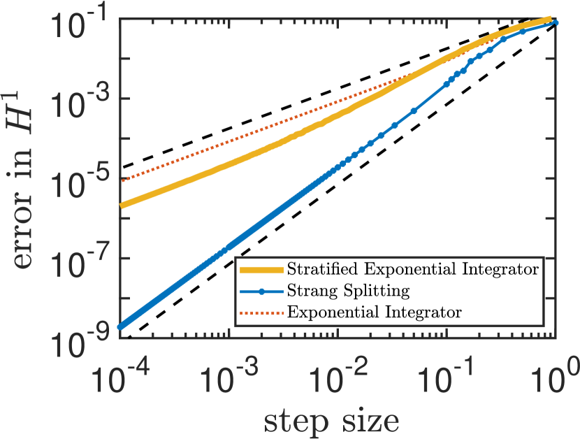
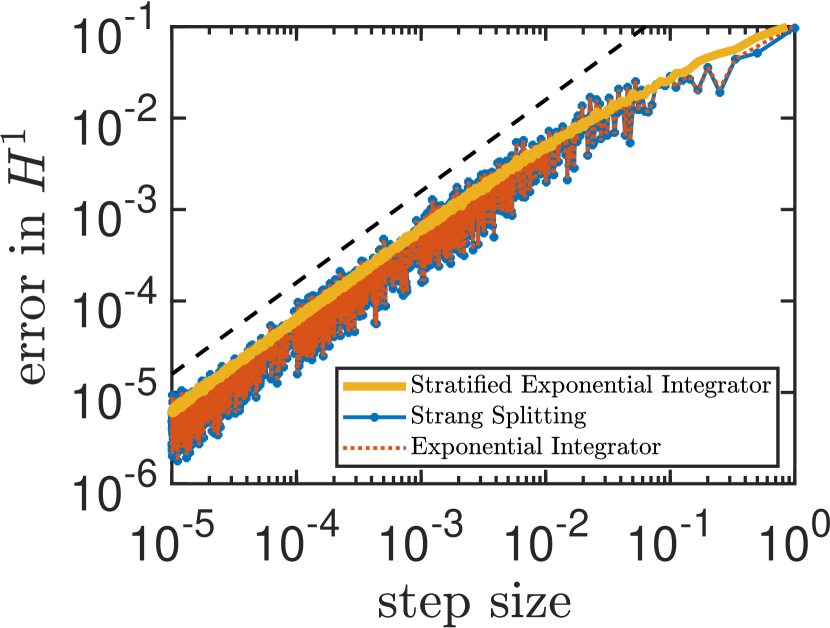
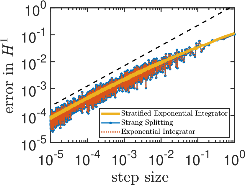
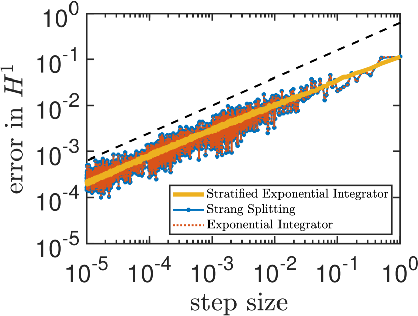
The numerical experiments emphasize the favorable error behavior of our newly derived scheme over classical integration methods in the presence of a non-smooth modulation $g$: Whereas the error of the classical schemes oscillates widely, reaching large errors, our proposed randomized exponential integrator (12) averages these oscillations and maintains its convergence rate at low regularity allowing smaller and in particular reliable errors without any oscillations.

In our numerical experiments we choose the classical exponential integrator

(25) $$u^{n+1}_{E}=U(t_{n}+\tau,t_{n})u^{n}_{E}-i\tau U(t_{n}+\tau,t_{n})\left(|u^{n}_{E}|^{2}u^{n}_{E}\right)$$

and Strang splitting scheme

(26) $$\psi^{n+1/2}_{-} =e^{-i\frac{\tau}{2}|\psi^{n+1}|^{2}}\psi^{n+1}$$

$$\psi^{n+1/2}_{+} =e^{i\left(g\left(t_{n+1}\right)-g\left(t_{n}\right)\right)\partial_{x}^{2}}\psi^{n+1/2}_{-}$$

$$\psi^{n+1} =e^{-i\frac{\tau}{2}|\psi^{n+1/2}_{+}|^{2}}\psi^{n+1/2}_{+}$$

associated to the modulated Schrödinger equation (1). In all numerical experiments we choose the initial value

$$u_{0}(x)=\frac{\mathrm{cos}(x)}{2-\mathrm{sin}(x)}$$

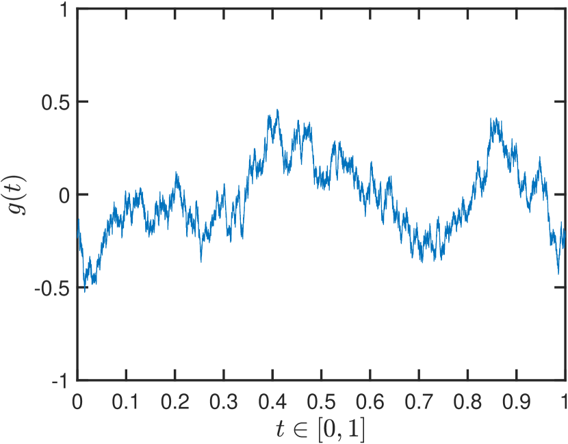
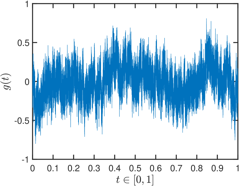
and use a standard Fourier pseudospectral method for the space discretization where we choose the largest Fourier mode $K=2^{7}$ (i.e., the spatial mesh size $\Delta x=0.049$). In the sequel, we use the notation $g$ in $W^{\alpha-,2}$ if $g\in W^{\gamma,2}$ for every $\gamma<\alpha$. To simulate modulations $g\in W^{\alpha-,2}$ , we first choose uniformly distributed random numbers in the interval $[-1,1]$, from which we take the discrete Fourier transform. These Fourier coefficients are then divided by $(1+|k|)^{\alpha+\frac{1}{2}}$ for $k=-\frac{N}{2},...,\frac{N}{2}-1$ and transformed back with the inverse Fourier transform and normalized. In Figure 1 below we illustrate the behavior of $g$ in two cases: $g\in W^{\frac{1}{2}-,2}$ and $g\in W^{\frac{1}{10}-,2}$.

(a) $g\in W^{\frac{1}{2}-,2}$

(b) $g\in W^{\frac{1}{10}-,2}$

Figure 1. Illustration of the behavior of the modulation function $g\in W^{\alpha-,2}$ in case of $\alpha=1/2$ and $\alpha=1/10$.

Moreover we consider a smooth example, where $g(t)=\mathrm{sin}(t)$. In the smooth setting $g(t)=\mathrm{sin}(t)$ we take as a reference solution the Strang splitting scheme with a very small time step size. In the less regular case of a function $g\in W^{\alpha-,2}$, i.e., for $\alpha=1/2$, $\alpha=1/4$ or $\alpha=1/10$ we take as a reference solution the schemes themselves with a very small time step size.
To compute the error $(\mathbb{E}\max_{M=0,\dots,N}\left\|e_{M}\right\|_{1}^{2})^{1/2}$ (see Theorem 3.1) of our randomized exponential integrator (12) we proceed as follows: We denote by $u^{\mathrm{ref}}(1)$ the reference solution at time $T=1$ and by $u_{(\xi_{i})_{i}^{k}}(1)$ the approximation computed with the randomized exponential integration scheme (12), by using the sequence $(\xi_{i})_{i}^{k}$. By taking $m\in\mathbb{N}$ sequences, we now use the approximation

$$\left(\mathbb{E}\max_{M=0,\dots,N}\left\|e_{M}\right\|_{1}^{2}\right)^{\frac{1}{2}}\approx\left(\frac{1}{m}\sum_{k=1}^{m}{\left\|u^{\mathrm{ref}}(1)-u_{(\xi_{i})_{i}^{k}}(1)\right\|_{1}^{2}}\right)^{\frac{1}{2}},$$

where the derivative is computed by means of the Fourier transform. Note that the new scheme can be easily implemented and allows for a parallelization in the sequence.
For the Strang splitting and the exponential integrator we compute the classical error in a discrete $H^{1}$ norm.

(a) $g(t)=\mathrm{sin}(t)$. The slope of the dashed lines is one and two, respectively.

(b) $g\in W^{\frac{1}{2}-,2}$. The slope of the dashed line is $\alpha+1/2=1$.

Figure 2. Convergence plot of the Strang splitting scheme (26), the classical exponential integrator (25) and the randomized exponential integrator (12) with $100$ sequences in the case of a smooth function $g$ (left) and a non-regular function $g\in W^{\frac{1}{2}-,2}$ (right).

(a) $g\in W^{\frac{1}{4}-,2}$. The slope of the dashed line is $\alpha+1/2=3/4$.

(b) $g\in W^{\frac{1}{10}-,2}$. The slope of the dashed line is $\alpha+1/2=3/5$.

Figure 3. Convergence plot of the Strang splitting scheme (26), the classical exponential integrator (25) and the randomized exponential integrator (12) with $100$ sequences in the case of a function $g\in W^{\alpha-,2}$ with different parameters $\alpha$.

References

• [1] F. Kh. Abdullaev, J. C. Bronski, and G. Papanicolaou, Soliton perturbations and the random Kepler problem. Physica D. Nonlinear Phenomena 135 (2000), no. 3-4, 369–386, DOI 10.1016/S0167-2789(99)00118-9.
• [2] A. Abdulle, G. Garegnani, Random time step probabilistic methods for uncertainty quantification in chaotic and geometric numerical integration. Preprint (2018) arXiv:1801.01340.
• [3] R. Belaouar, A. de Bouard, A. Debussche, Numerical analysis of the nonlinear Schrödinger equation with white noise dispersion. Stochastic Partial Differential Equations: Analysis and Computations, 3, 1, pp. 103–132 (2015).
• [4] C. Besse, B. Bidégaray, S. Descombes, Order estimates in time of splitting methods for the nonlinear Schrödinger equation. SIAM J. Numer. Anal. 40:26–40 (2002).
• [5] D. L. Burkholder, Martingale transforms. Ann. Math. Statist., 37:1494–1504 (1966).
• [6] E. Celledoni, D. Cohen, B. Owren, Symmetric exponential integrators with an application to the cubic Schrödinger equation. Found. Comput. Math. 8:303–317 (2008).
• [7] K. Chouk, M. Gubinelli, Nonlinear PDEs with modulated dispersion I: Nonlinear Schrödinger equations. Communications in Partial Differential Equations. 2015.40(11):2047–81.
• [8] D. Cohen, G. Dujardin, Exponential integrators for nonlinear Schrödinger equations with white noise dispersion. Stochastics and Partial Differential Equations: Analysis and Computations, to appear.
• [9] D. Cohen, L. Gauckler, One-stage exponential integrators for nonlinear Schrödinger equations over long times. BIT 52:877–903 (2012).
• [10] A. de Bouard and A. Debussche, The nonlinear Schrödinger equation with white noise dispersion. Journal of Functional Analysis 259 (5) 1300–1321 (2010).
• [11] A. Debussche and Y. Tsutsumi, 1D quintic nonlinear Schrödinger equation with white noise dispersion. Journal de Mathématiques Pures et Appliquées 96 4) 363–376 (2011).
• [12] G. Dujardin, Exponential Runge-Kutta methods for the Schrödinger equation. Appl. Numer. Math. 59:1839–1857 (2009).
• [13] B. Engquist, A. Fokas, E. Hairer, A. Iserles, Highly Oscillatory Problems. Cambridge University Press, 2009
• [14] M. Eisenmann, M. Kovács, R. Kruse, S. Larsson, On a randomized, backward Euler method for nonlinear evolution equations with time-irregular coefficients. arXiv:1709:01018.
• [15] E. Faou, Geometric Numerical Integration and Schrödinger Equations. European Math. Soc. Publishing House, Zürich 2012.
• [16] L. Gauckler, Convergence of a split-step Hermite method for the Gross–Pitaevskii equation. IMA J. Numer. Anal. 31:396–415 (2011).
• [17] E. Hairer, C. Lubich, G. Wanner, Geometric Numerical Integration. Structure-Preserving Algorithms for Ordinary Differential Equations. Second edition, Springer, Berlin 2006.
• [18] M. Hochbruck, A. Ostermann, Exponential integrators. Acta Numer. 19:209–286 (2010).
• [19] H. Holden, K. H. Karlsen, K.-A. Lie, N. H. Risebro, Splitting for Partial Differential Equations with Rough Solutions. European Math. Soc. Publishing House, Zürich 2010.
• [20] D. Hundertmark, Y. R. Lee, Decay estimates and smoothness for solutions of the dispersion managed nonlinear Schrdinger equation. Communications in Mathematical Physics 286 (3) 851–873 (2009).
• [21] D. Hundertmark, Y. R. Lee, Super-exponential decay of diffraction managed solitons. Communications inMathematical Physics 309 (1) 1–21 (2012).
• [22] P. Bader, A. Iserles, K. Kropielnicka, P. Singh, Effective Approximation for the Semiclassical Schrödinger Equation. Foundations of Computational Mathematics 14 689–720 (2014).
• [23] S. Jin, P. Markowich, C. Sparber, Mathematical and computational methods for semiclassical Schrödinger equations. Acta Numer. 20 121–210 (2011).
• [24] A. Jentzen and A. Neuenkirch, A random Euler scheme for Carathéodory differential equations. J. Comput. Appl. Math., 224(1):346–359, 2009.
• [25] M. Kunze, J. Moeser, V. Zharnitsky, Ground states for the higher-order dispersion managed NLS equation in the absence of average dispersion. Journal of Differential Equations 209 (1) 77–100 (2005).
• [26] R. Kruse and Y. Wu, Error analysis of randomized Runge-Kutta methods for differential equations with time-irregular coefficients. Comput. Methods Appl. Math., 17(3):479–498, 2017.
• [27] R. Kruse and Y. Wu, A randomized Milstein method for stochastic differential equations with non-differentiable drift coefficients. arXiv:1706:09964.
• [28] C. Lubich, On splitting methods for Schrödinger–Poisson and cubic nonlinear Schrödinger equations. Math. Comp. 77:2141–2153 (2008).
• [29] R. Marty, On a splitting scheme for the nonlinear Schrödinger equation in a random medium. Communications in Mathematical Sciences 4 (4) 679–705(2006).
• [30] R.I. McLachlan, G.R.W. Quispel, Splitting methods, Acta Numer. 11:341–434 (2002).
• [31] V. Schmidt, Stochastic Geometry, Spatial Statistics and Random Fields, Models and Algorithms, Springer International Publishing Switzerland, 2015
• [32] V. Zharnitsky, E. Grenier, C. K.R.T. Jones, and S. K. Turitsyn, Stabilizing effects of dispersion management. Physica D: Nonlinear Phenomena 152-153 794–817 (2001).