Order reduction approaches for the algebraic Riccati equation and the LQR problem

Abstract

We explore order reduction techniques for solving the algebraic Riccati equation (ARE), and investigating the numerical solution of the linear-quadratic regulator problem (LQR). A classical approach is to build a surrogate low dimensional model of the dynamical system, for instance by means of balanced truncation, and then solve the corresponding ARE. Alternatively, iterative methods can be used to directly solve the ARE and use its approximate solution to estimate quantities associated with the LQR. We propose a class of Petrov-Galerkin strategies that simultaneously reduce the dynamical system while approximately solving the ARE by projection. This methodology significantly generalizes a recently developed Galerkin method by using a pair of projection spaces, as it is often done in model order reduction of dynamical systems. Numerical experiments illustrate the advantages of the new class of methods over classical approaches when dealing with large matrices.

1 Introduction

Optimal control problems for partial differential equations (PDEs) are an extremely important topic for many industrial applications in different fields, from aerospace engineering to economics. The problem has been investigated with different strategies as open-loop (see e.g. HPUU09 ) or closed-loop (see e.g. AFV17 ; FF14 ; GP11 ).

In this work we are interested in feedback control for linear dynamical systems and quadratic cost functional which is known as the Linear Quadratic Regulator (LQR) problem. Although most models are nonlinear, LQR is still a very interesting and powerful tool, for instance in the stabilization of nonlinear models under perturbations, where a control in feedback form can be employed.

The computation of the optimal policy in LQR problems requires the solution of an algebraic Riccati equation (ARE), a quadratic matrix equation with the dimension of the dynamical system. This is a major bottleneck in the numerical treatment of the optimal control problem, especially for high dimensional systems such as those stemming from the discretization of a three-dimensional PDE.

Several powerful solution methods for the ARE have been developed throughout the years for small dynamical systems, based on spectral decompositions. The large scale case is far more challenging, as the whole spectral space of the relevant matrices cannot be determined because of memory and computational resource limitations. For these reasons, this algebraic problem is a very active research topic, and major contributions have been given in the past decade. Different approaches have been explored: variants of the Newton method have been largely employed in the past K68 ,BS10 , while only more recently reduction type methods have emerged as a feasible effective alternative; see, e.g., Benner.Saak.survey13 ,SSM14 and references therein. The recent work Simoncini2016 shows that a Galerkin class of reduction methods for solving the ARE can be naturally set into the framework of model order reduction for the original dynamical system.

As already mentioned, the LQR problem is more complicated when dealing with PDEs because its discretization leads to a very large system of ODEs and, as a consequence, the numerical solution of the ARE is computationally more demanding. To significantly lower these computational costs and memory requirements, model order reduction techniques can be employed. Here, we distinguish between two different concepts of reduction approaches.

A first methodology projects the dynamical system into a low dimensional system whose dimensions are much smaller than the original one; see, e.g., BCOW.17 . Therefore, the corresponding reduced ARE is practical and feasible to compute on a standard computer. The overall methodology thus performs a first-reduce-then-solve strategy. This approach has been investigated with different model reduction techniques like Balanced Truncation (bt) in e.g.A05 , Proper Orthogonal Decomposition (pod, Sir87 ; Vol11 ) in e.g. AK01 ; KS16 and via the interpolation of the rational functions, see Gugercin2008a ,GB17 , bG15 . A different approach has been proposed in SH17 where the basis functions are computed from the solution of the high dimensional Riccati equation in a many query context. We note that basis generation in the context of model order reduction for optimal control problems is an active research topic (see e.g. AGH16 ; ASH17 ; KS16 ; KV08 ). Furthermore, the computation of the basis functions is made by a Singular Value Decomposition (SVD) of the high dimensional data which can be very expensive. One way to overcome this issue was proposed in AK17 by means of randomized SVD which is a fast and accurate alternative to the SVD, and it is based on random samplings.

A second methodology follows a reduce-while-solve strategy. In this context, recent developments aim at reducing the original problem by subspace projection, and determining an approximate solution in a low dimensional approximation space. Proposed strategies either explicitly reduce the quadratic equation (see, e.g., SSM14 and references therein), or approximately solve the associated invariant subspace problem (see, e.g., Benner.Bujanovic.16 and its references). As already mentioned, these recently developed methods have shown to be effective alternatives to classical variants of the Newton method, which require the solution of a linear matrix equation at each nonlinear iteration; see, e.g., Benner.Li.Penzl.08 for a general description.

The aim of this paper is to discuss and compare the aforementioned model order reduction methodologies for LQR problems. In particular, we compare the two approaches of reducing the dynamical system first versus building surrogate approximation of the ARE directly, using either Galerkin or Petrov-Galerkin projections. The idea of using a Petrov-Galerkin method for the ARE appears to be new, and naturally expands the use of two-bases type order reduction methods typically employed for transfer function approximation.

To set the paper into perspective we start recalling LQR problem and its order reduction in Section 2. In Section 3 we describe reduction strategies of dynamical systems used in the small size case, such as proper orthogonal decomposition and balanced truncation. Section 4 discusses the new class of projection strategies that attack the Riccati equation, while delivering a reduced order model for the dynamical system. Finally, numerical experiments are shown in Section 5 and conclusions are derived in Section 6.

2 The linear-quadratic regulator problem and model order reduction

In this section we recall the mathematical formulation of the LQR problem. We refer the reader for instance to classical books such as e.g. Lancaster.Rodman.95 for a comprehensive description of what follows. We consider a linear time invariant system of ordinary differential equations of dimension $n$:

$$\dot{x}(t) =Ax(t)+Bu(t),\quad x(0)=x_{0},\quad t>0,$$ (1)

$$y(t) =Cx(t)+Du(t),$$

with $A\in\mathbb{R}^{n\times n},B\in\mathbb{R}^{n\times m},C\in\mathbb{R}^{p\times n}$ and $D\in\mathbb{R}^{p\times m}$. Usually, $x(t):[0,\infty]\rightarrow\mathbb{R}^{n}$ is called the state, $u(t):[0,\infty]\rightarrow\mathbb{R}^{m}$ the input or control and $y(t):[0,\infty]\rightarrow\mathbb{R}^{p}$ the output. Furthermore, we assume that $A$ is passive. This may be viewed as a restrictive hypothesis, since the problems we consider only require that $(A,B)$ are stabilizable and $(C,A^{T})$ controllable, however this is convenient to ensure that the methods we analyze are well defined. In what follows, without loss of generality, we will consider $D\equiv 0$. We also define the transfer function for later use:

$$G(s)=C(sI-A)^{-1}B.$$ (2)

Next, we define the quadratic cost functional for an infinite horizon problem:

$$J(u):=\int_{0}^{\infty}y(t)^{T}y(t)+u(t)^{T}Ru(t)\,dt,$$ (3)

where $R\in\mathbb{R}^{m\times m}$ is a symmetric positive definite matrix. The optimal control problem reads:

$$\min_{u\in\mathbb{R}^{m}}J(u)\quad\text{such that}\quad x(t)\quad\mbox{ solves }\quad\eqref{sys}.$$ (4)

The goal is to find a control policy in feedback form as:

$$u(t)=-Kx(t)=-R^{-1}B^{T}Px(t)$$ (5)

with the feedback gain matrix $K\in\mathbb{R}^{m\times n}$ and $P\in\mathbb{R}^{n\times n}$ is the unique symmetric and positive (semi-)definite matrix that solves the following ARE:

$$A^{T}P+PA-PBR^{-1}B^{T}P+C^{T}C=0,$$ (6)

which is a quadratic matrix equation for the unknown $P$.

We note that the numerical approximation of equation (6) can be very expensive for large $n$. Therefore, we aim at the reduction of the numerical complexity by projection methods.

Let us consider a general class of tall matrices $V,W\in\mathbb{R}^{n\times r}$, whose columns span some approximation spaces. We chose these two matrices such that they are biorthogonal, that is $W^{T}V=I_{r}$. Let us now assume that the matrix $P$, solution of (6), can be approximated as

$$P\approx WP_{r}W^{T}.$$

Then the residual matrix can be defined as

$$\mathcal{R}(P_{r})=A^{T}WP_{r}W^{T}+WP_{r}W^{T}A-WP_{r}W^{T}BR^{-1}B^{T}WP_{r}W^{T}+C^{T}C.$$

The small dimensional matrix $P_{r}$ can be determined by imposing the so-called Petrov-Galerkin condition, that is orthogonality of the residual with respect to range$(V)$, which in matrix terms can be stated as $V^{T}\mathcal{R}(P_{r})V=0$. Substituting the residual matrix and exploiting the bi-orthogonality of $V$ and $W$ we obtain:

$$A_{r}^{T}P_{r}+P_{r}A_{r}-P_{r}B_{r}R^{-1}B_{r}^{T}P_{r}+C_{r}^{T}C_{r}=0$$ (7)

where

$$A_{r}=W^{T}AV,\quad B_{r}=W^{T}B,\quad C_{r}=CV.$$

It can be readily seen that equation (7) is again a matrix Riccati equation, in the unknown matrix $P_{r}\in\mathbb{R}^{r\times r}$, of much smaller dimension than $P$, provided that $V$ and $W$ generate small spaces. We refer to this equation as the reduced Riccati equation. The computation of $P_{r}$ allows us to formally obtain the approximate solution $WP_{r}W^{T}$ to the original Riccati equation (6), although the actual product is never computed explicitly, as the approximation is kept in factorized form.

The optimal control for the reduced problem reads

$$u_{r}(t)=-K_{r}x_{r}(t)=-R^{-1}B_{r}^{T}P_{r}x_{r}(t)$$

with the reduced feedback gain matrix given by $K_{r}=KV\in\mathbb{R}^{m\times r}$. Note that this $u_{r}(t)$ is different from the one obtained by first approximately solving the Riccati equation and with the obtained matrix defining an approximation to $u(t)$; see Simoncini2016 for a detailed discussion.

The Galerkin approach is obtained by choosing $V=W$ with orthonormal columns when imposing the condition on the residual.

To reduce the dimension of the dynamical system (1), we assume to approximate the full state vector as $x(t)\approx Vx_{r}(t)$ with a basis matrix $V\in\mathbb{R}^{n\times r}$, where $x_{r}(t):[0,\infty)\rightarrow\mathbb{R}^{r}$ are the reduced coordinates. Plugging this ansatz into the dynamical system (1), and requiring a so called Petrov-Galerkin condition yields

$$\dot{x}_{r}(t) = A_{r}x_{r}(t)+B_{r}u(t),\quad x_{r}(0)=W^{T}x_{0},\quad t>0,$$ (8)

$$y_{r}(t) = C_{r}x_{r}.$$

The reduced transfer function is then given by:

$$G_{r}(s)=C_{r}(sI_{r}-A_{r})^{-1}B_{r}.$$ (9)

The presented procedure is a generic framework for model reduction. It is clear that the quality of the approximation depends on the approximation properties of the reduced spaces. In the following sections, we will distinguish between the methods that directly compute $V,W$ upon the dynamical systems (see Section 3) and those that readily reduce the ARE (see Section 4). In particular, for each method we will discuss both Galerkin and Petrov-Galerkin projections, to provide a complete overview of the methodology. The considered general Petrov-Galerkin approach for the ARE appears to be new.

3 Reduction of the dynamical system

In this section we recall two well-known techniques as pod and bt to compute the projectors $W,V$ starting from the dynamical systems.

3.1 Proper Orthogonal Decomposition

A common approach is based on the snapshot form of pod proposed in Sir87 , which works as follows. We compute a set of snapshots $x(t_{1}),\dots,x(t_{k})$ of the dynamical system (1) corresponding to a prescribed input $\bar{u}(t)$ and different time instances $t_{1},\ldots,t_{k}$ and define the pod ansatz of order $r$ for the state $x(t)$ by

$$x(t)\approx\sum_{i=1}^{r}{(x_{r})}_{i}(t)\psi_{i},$$ (10)

where the basis vectors $\{\psi_{i}\}_{i=1}^{r}$ are obtained from the SVD of the snapshot matrix $X=[x(t_{1}),\ldots,x(t_{k})],$ i.e. $X=\Psi\Sigma\Gamma^{T}$, and the first $r$ columns of $\Psi=(\Psi_{1},\dots,\Psi_{n})$ form the pod basis functions of rank $r$. Hence we choose the basis vectors $V=W=(\Psi_{1},\dots,\Psi_{r})$ for the reduction in (8). This technique strongly relies on the choice of a given input $u$, whose optimal selection is usually unknown. In this work, we decide to collect snapshots following the approach suggested in KS16 as considers a linearization of the ARE (which corresponds to a Lyapunov equation). Therefore, the snapshots are computed by the following equation:

$$\dot{x}(t)=A^{T}x(t),\quad x(0)=c_{i},\quad\text{for }i=1,\ldots p$$ (11)

where $c_{i}$ is the $i-$th column of the matrix $C$. The advantage of this approach is that equation (11) is able to capture the dynamics of the adjoint equation which is directly related to the optimality conditions, and we do not have to chose a reference input $\bar{u}(t).$ In order to obtain the pod basis, one has to simulate the high dimensional system and subsequently perform a SVD. As a consequence, the computational cost may become prohibitive for large scale problems. Algorithm 1 summarizes the method.

Algorithm 1 pod method to compute the reduced Riccati

0:  $A,C,r$

1:  for $i=1,\ldots,p$ do

2:     Simulate system (11) with initial condition $c_{i}$.

3:     Build the snapshots matrix $X=[X,x_{i}(t_{1}),\ldots,x_{i}(t_{k})]$

4:  end for

5:  Compute the reduced SVD of $X=V\Sigma W^{T}$

6:  Solve the reduced Riccati equation (7) for $P_{r}$.

3.2 Balanced truncation

The bt method is a well-established reduced order modeling technique for linear time invariant systems (1). We refer to A05 for a complete description of the topic. It is based on the solution of the reachability Gramian $R$ and the observability Gramian $O$ which solve, respectively, the following Lyapunov equations

$$AR+RA^{T}+BB^{T}=0,\quad A^{T}O+OA+C^{T}C=0.$$ (12)

We determine the Cholesky factorization of the Gramians

$$R=\Phi\Phi^{T}\qquad O=\Upsilon\Upsilon^{T}.$$ (13)

Then, we compute the reduced SVD of the Hankel operator $\Upsilon^{T}\Phi$ and set

$$W=\Upsilon U\Sigma^{1/2},\qquad V=\Upsilon V\Sigma^{1/2},$$

where $U,V\in\mathbb{R}^{n\times r}$ are the first $r$ columns of the left and right singular vectors of the Hankel operator and $\Sigma=\mbox{diag}(\sigma_{1},\ldots,\sigma_{r})$ matrix of the first $r$ singular values.

The idea of bt is to neglect states that are both, hard to reach and hard to observe. This is done by eliminating states that correspond to low Hankel singular values $\sigma_{i}$. This method is very popular in the small case regime, also because the whole procedure can be verified by a-priori error bounds in several system norms, and the Lyapunov equations can be solved very efficiently. In the large scale these equations need to be solved approximately; see, e.g.,  Benner.Saak.survey13 .

In summary, the procedure first solves the two Lyapunov equations at a given accuracy and then determines biorthogonal bases for the reduction spaces by using a combined spectral decomposition of the obtained solution matrices. We note that this method is also very expensive for large $n$. The algorithm is summarized below in Algorithm 2.

Algorithm 2 bt method to compute the reduced Riccati

0:  $A,B,C$ and the dimension of the reduced problem $r$

1:  Compute $R,O$ from (12) and their Cholesky factorization (13)

2:  Compute the reduced SVD of the Hankel operator

3:  Set $W=\Upsilon U\Sigma^{1/2},\qquad V=\Upsilon V\Sigma^{1/2},$

4:  Solve the reduced Riccati equation (7) for $P_{r}$.

4 Adaptive reduction of the algebraic Riccati equation

In the previous section the reduced problem was obtained by a sequential procedure: first system reduction of a fixed order $r$ and then solution of the reduced Riccati equation (7). A rather different strategy consists of determining the reduction bases while solving the Riccati equation. In this way, we combine both the reduction of the original system and of the ARE. While the reduction bases $V$ and $W$ are being generated by means of some iterative strategy, it is immediately possible to obtain a reduced Riccati equation by projecting the problem onto the current approximation spaces. The quality of the two spaces can be monitored by checking how well the Riccati equation is solved by means of its residual; if the approximation is not satisfactory, the spaces can be expanded and the approximation improved.

The actual space dimensions are not chosen a-priori, but tailored with the accuracy of the approximate Riccati solution. Mimicking what is currently available in the linear equation literature, the reduced problem can be obtained by imposing some constraints that uniquely identify an approximation. The idea is very natural and it was indeed presented in JaimoukhaFeb.1994 , where a standard Krylov basis was used as approximation space. However, only more recently, with the use of rational Krylov bases, a Galerkin approach has shown its real potential as a solver for the Riccati equation; see, e.g., Heyouni.Jbilou.09 ,SSM14 . A more general Petrov-Galerkin approach was missing. We aim to fill this gap. In the following we give more details on these procedures.

Given an approximate solution $\tilde{P}$ of (6) written as $\tilde{P}=WYW^{T}$ for some $Y$ to be determined, the former consists to require that the residual matrix is orthogonal to this same space, range($W$), so that in practice $V=W$. The Petrov-Galerkin procedure imposes orthogonality with respect to the space range($V$), where $V$ is different from $W$, but with the same number of columns.

In JaimoukhaFeb.1994 a first implementation of a Galerkin procedure was introduced, and the orthonormal columns of $V$ spanning the (block) Krylov subspace ${\cal K}_{r}(A^{T},C^{T})={\rm range}([C^{T},A^{T}C^{T},\ldots,(A^{T})^{r-1}C^{T}])$; see also Jbilou_03 for a more detailed treatment and for numerical experiments. Clearly, this definition generates a sequence of nested approximation spaces, that is ${\cal K}_{r}(A^{T},C^{T})\subseteq{\cal K}_{r+1}(A^{T},C^{T})$, whose dimension can be increased iteratively until a desired accuracy is achieved. More recently, in Heyouni.Jbilou.09 and SSM14 , rational Krylov subspaces have been used, again in the Galerkin framework. In particular, the special case of the extended Krylov subspace ${\cal K}_{r}(A^{T},C^{T})+{\cal K}_{r}((A^{T})^{-1},(A^{T})^{-1}C^{T})$ was discussed in Heyouni.Jbilou.09 , while the fully rational space

$${\cal K}_{r}(A^{T},C^{T},{\boldsymbol{\sigma}}):={\rm range}([C^{T},(A^{T}-\sigma_{2}I)^{-1}C^{T},\ldots,(A^{T}-\sigma_{2}I)^{-1}\cdots(A^{T}-\sigma_{r}I)^{-1}C^{T}])$$

was used in SSM14 . The rational shift parameters ${\boldsymbol{\sigma}}=\{\sigma_{2},\ldots,\sigma_{r}\}$ can be computed on the fly at low cost, by adapting the selection to the current approximation quality Druskin.Simoncini.11 . Note that dim(${\cal K}_{r}(A^{T},C^{T},{\boldsymbol{\sigma}}))\leq rp$, where $p$ is the number of columns of $C^{T}$. In SSM14 it was also shown that a fully rational space can be more beneficial than the extended Krylov subspace for the Riccati equation. In the following section we are going to recall the general procedure associated with the Galerkin approach, and introduce the algorithm for the Petrov-Galerkin method, which to the best of the authors’ knowledge is new. In both cases we use the fully rational Krylov subspace with adaptive choice of the shifts.

It is important to realize that ${\cal K}_{r}(A^{T},C^{T},{\boldsymbol{\sigma}})$ does not depend on the coefficient matrix $BB^{T}$ of the second-order term in the Riccati equation. Nonetheless, experimental evidence shows good performance. This issue was analyzed in Lin.Simoncini.15 ; Simoncini.16 where however the use of the matrix $B$ during the computation of the parameters was found to be particularly effective; a justification of this behavior was given in Simoncini.16 . In the following we thus employ this last variant when using rational Krylov subspaces. More details will be given in the next section.

4.1 Galerkin and Petrov-Galerkin Riccati

In the Galerkin case, we will generate a matrix $W$ whose columns span the rational Krylov subspace ${\cal K}_{r}(A^{T},C^{T},{\boldsymbol{\sigma}})$ in an iterative way, that is one block of columns at the time. This can be obtained by an Arnoldi-type procedure; see, e.g., A05 . The algorithm, hereafter gark for Galerkin Adaptive Rational Krylov, works as follows:

Algorithm 3 gark method to compute the reduced Riccati equation

0:  $A,C,\boldsymbol{\sigma}$

1:  for $r=1,2,\ldots$ do

2:     Expand the space ${\cal K}_{r}(A^{T},C^{T},{\boldsymbol{\sigma}})$;

3:     Update the reduced matrices $A_{r},B_{r}$ and $C_{r}$ with the newly generated vectors;

4:     Solve the reduced Riccati equation for $P_{r}$;

5:     Check the norm of the residual matrix ${\cal R}(P_{r})$

6:     If satisfied stop with $P^{r}$ and the basis $W$ of ${\cal K}_{r}(A^{T},C^{T},{\boldsymbol{\sigma}})$.

7:  end for

The residual norm can be computed cheaply without the actual computation of the residual matrix; see, e.g., SSM14 . The parameters $\sigma_{j}$ can be computed adaptively as the space grows; we refer the reader to Druskin.Simoncini.11 and Simoncini.16 for more details.

In the general Petrov-Galerkin case, the matrix $W$ is generated the same way, while we propose to compute the columns of $V$ as the basis for the rational Krylov subspace ${\cal K}_{r}(A,B,{\boldsymbol{\sigma}})$; note that the starting block is now $B$, and the coefficient matrix is the transpose of the previous one. The two spaces are now constructed and expanded at the same time, so that the two bases can be enforced to be biorthogonal while they grow. For completeness, we report the algorithm in the Petrov-Galerkin setting in Algorithm 4 (hereafter pgark for Petrov-Galerkin Adaptive Rational Krylov).

Algorithm 4 pgark method to compute the reduced Riccati equation

0:  $A,B,C,\boldsymbol{\sigma}$

1:  for $r=1,2,\ldots$ do

2:     Expand the spaces ${\cal K}_{r}(A^{T},C^{T},{\boldsymbol{\sigma}})$, ${\cal K}_{r}(A,B,{\boldsymbol{\sigma}})$;

3:     Update the reduced matrices $A_{r},B_{r}$ and $C_{r}$ with the newly generated vectors;

4:     Solve the reduced Riccati equation for $P_{r}$;

5:     Check the norm of the residual matrix ${\cal R}(P_{r})$

6:     If satisfied stop with $P^{r}$ and the basis $W$ of ${\cal K}_{r}(A^{T},C^{T},{\boldsymbol{\sigma}})$.

7:  end for

The parameters $\sigma_{j}$ are computed for one space and used also for the other space. In this more general case, the formula for the residual matrix norm is not as cheap as for the Galerkin approach. We suggest the following procedure. We first recall that for rational Krylov subspace ${\cal K}_{r}(A,B,{\boldsymbol{\sigma}})$ the following relation holds (we assume here full dimension of the generated space after $r$ iterations):

$$A^{T}W=WA_{r}+\hat{w}a_{r}^{T},\quad{a_{r}}\in\mathbb{R}^{(r+1)m},$$

for certain vector $\hat{w}$ orthogonal to $W$, which changes as the iterations proceeds, that is as the number of columns $W$ grows; we refer the reader to Lin.Simoncini.12 for a derivation of this relation, which highlights that the distance of range($W$) from an invariant subspace of $A$ is measured in terms of a rank-one matrix. We write

$$\mathcal{R}(P_{r}) = A^{T}WP_{r}W^{T}+WP_{r}W^{T}A-WP_{r}W^{T}BR^{-1}B^{T}WP_{r}W^{T}+C^{T}C$$

$$= WA_{r}P_{r}W^{T}+\hat{w}a_{r}^{T}P_{r}W^{T}+WP_{r}A_{r}^{T}W^{T}+WP_{r}a_{r}\hat{w}^{T}-WP_{r}B_{r}R^{-1}B_{r}^{T}P_{r}W^{T}+WEE^{T}W^{T}$$

$$= \hat{w}a_{r}^{T}P_{r}W^{T}+WP_{r}a_{r}\hat{w}^{T}$$

$$= [W,\hat{w}]\begin{bmatrix}0&P_{r}a_{r}\\ a_{r}^{T}P_{r}&0\end{bmatrix}[W,\hat{w}]^{T},$$

where we also used the fact that $C^{T}=WE$ for some matrix $E$. If $[W,\hat{w}]$ had orthonormal columns, as is the case for Galerkin, then $\|{\mathcal{R}}(P_{r})\|^{2}=2\|P_{r}a_{r}\|^{2}$, which can be cheaply computed.

To overcome the nonorthogonality of $[W,\hat{w}]$, we suggest to perform a reduced QR factorization of $[W,\hat{w}]$ that maintains its columns orthogonal. This QR factorization does not have to be redone from scratch at each iteration, but it can be updated as the matrix $W$ grows. If $[W,\hat{w}]=Q_{W}R_{W}$ with $R_{W}\in\mathbb{R}^{(r+1)m\times(r+1)m}$ upper triangular, then

$$\|{\cal R}(P_{r})\|=\|R_{W}\begin{bmatrix}0&P_{r}a_{r}\\ a_{r}^{T}P_{r}&0\end{bmatrix}R_{W}^{T}\|.$$

The use of coupled (bi-orthogonal) bases has the recognized advantage of explicitly using both matrices $C$ and $B$ in the construction of the reduced spaces. This coupled basis approach has been largely exploited in the approximation of the dynamical system transfer function by solving a multipoint interpolation problem; see, e.g., A05 for a general treatment and Barkouki2015 for a recent implementation. In addition, coupled bases can be used to simultaneously approximate both system Gramians leading to a large-scale bt strategy; see, e.g., Jaimoukha.Kasenally.95 for early contributions using bi-orthogonal standard Krylov subspaces. On the other hand, a Petrov-Galerkin procedure has several drawbacks associated with the construction of the two bases. More precisely, the two bi-orthogonal bases are generated by means of a Lanczos-type recurrence, which is known to have both stability and breakdown problems in other contexts such as linear system and eigenvalue solving. At any iteration it may happen that the new basis vectors $w_{j}$ and $v_{j}$ are actually orthogonal or quasi-orthogonal to each other, giving rise to a possibly incurable breakdown GutknechtApr.1992 . We have occasionally experienced this problem in our numerical tests, and it certainly occurs whenever $CB=0$. In our specific context, an additional difficulty arises. The projected matrix $A_{r}=W^{T}A^{T}V$ is associated with a bilinear rather than a linear form, so that its field of values may be unrelated to that of $A^{T}$. As a consequence, it is not clear the type of hypotheses we need to impose on the data to ensure that the reduced Riccati equation (7) admits a unique stabilizable solution. Even in the case of $A$ symmetric, the two bases will be different as long as $C\neq B^{T}$. All these questions are crucial for the robustness of the procedure and deserve a more throughout analysis which will be the topic of future research.

From an energy-saving standpoint, it is worth remarking that the Petrov-Galerkin approach uses twice as many memory allocations than the Galerkin approach, while performing about twice the number of floating point operations. In particular, constructing the two bases requires two system solves, with $A^{T}-s_{j}I$ and with $A-\bar{s}_{j}I$ respectively, at each iteration. Therefore, unless convergence is considerably faster, the Petrov-Galerkin approach may not be superior to the Galerkin method in the solution of the ARE.

5 Numerical Experiments

In this section we present and discuss our numerical tests. We consider the discretization of the following linear PDE

$$w_{t}-\varepsilon\Delta w+\gamma w_{x}+\gamma w_{y} =\mathbf{1}_{\Omega_{B}}u \text{in }\Omega\times(0,+\infty),$$ (14)

$$w(\cdot,0) =w_{0} \text{in }\Omega,$$

$$w(\cdot,t) =0 \text{in }\partial\Omega\times(0,\infty),$$

where $\Omega\subset\mathbb{R}^{2}$ is an open interval, $w:\Omega\times[0,\infty]\rightarrow\mathbb{R}^{2}$ denotes the state, and the parameters $\varepsilon$ and $\gamma$ are real positive constants. The initial value is $w_{0}$ and the function $\mathbf{1}_{\Omega_{B}}$ is the indicator function over the domain $\Omega_{B}\subset\mathbb{R}^{2}$. Note that we deal with zero Dirichlet boundary conditions. The problem in (14) includes the heat equation, for $\varepsilon\neq 0,\gamma=0$, and a class of convection-diffusion equations for $\varepsilon\neq 0$ and $\gamma\neq 0$. Furthermore, we define an output of interest by:

$$s(t):=\dfrac{1}{|\Omega_{C}|}\int_{\Omega_{C}}w(x,t)\,dt,$$ (15)

where $\Omega_{C}\subset\mathbb{R}^{2}.$ Space discretization of equation (14) by standard centered finite differences together with a rectangular quadrature rule for (15) lead to a system of the form (1). In general, the dimension $n$ of the dynamical system (1) is rather large (i.e., $n\gg 1000$) and the numerical treatment of the corresponding ARE is computationally expensive or even unfeasible. Therefore, model order reduction is appropriate to lower the dimension of the optimal control problem (4). We will report experiments with small size problems, where all discussed methods can be employed, and with large size problems, where only the Krylov subspace based strategies are applied.

The numerical simulations reported in this paper were performed on a Mac-Book Pro with 1 CPU Intel Core i5 2.3 Ghz and 8GB RAM and the codes are written in MatlabR2013a. In all our experiments, small dimensional Lyapunov and Riccati equations are solved by means of built-in functions of the Matlab Control Toolbox.

Whenever appropriate, the quality of the current approximation of the ARE is monitored by using the relative residual norm:

$${\tt R}_{P}=\dfrac{\|\mathcal{R}(P_{r})\|_{F}}{\|C\|_{F}^{2}},$$ (16)

and the dimension of the surrogate model $r$ is chosen such that ${\tt R}_{P}<10^{-8}$. After the ARE solution is approximated the ultimate goal is to compute the feedback control (5). Therefore, we also report the error in the computation of feedback gain matrix $K$ as the iterations proceed:

$$\mathcal{E}_{K}=\dfrac{\|K_{r}-K\|_{F}}{\|K\|_{F}},$$ (17)

and we measure the quality of our surrogate model also by the $\mathcal{H}_{2}-$ error

$$\mathcal{E}_{G}=\dfrac{\|G_{r}-G\|_{\mathcal{H}_{2}}}{\|G\|_{\mathcal{H}_{2}}}.$$ (18)

where

$$\|G(s)\|_{\mathcal{H}_{2}}:=\dfrac{1}{2\pi}\left(\int_{-\infty}^{+\infty}\|G(i\omega)\|_{F}^{2}d\omega\right)^{1/2}.$$

In particular, the approximation of the transfer function is one of the main targets of reduced order modeling, where the reduced system is used for analysis purposes, while the approximation of the feedback gain matrix is monitored to obtain a good control function.

5.1 Test 1: 2D Linear heat equation

In the first example we consider the linear heat equation. In (14) we chose $\gamma=0,\varepsilon=1,\Omega=[0,1]\times[0,1],$ and $\Omega_{B}=[0.2,0.8]\times[0.2,0.8]$. In (1), the matrix $A$ is obtained by centered five points discretization. We consider a small problem stemming from a spatial discretization step $\Delta x=0.05$, leading to a system of dimension $n=441$. The matrix $C$ in (1) is given by the indicator function over the domain $\Omega_{C}=[0.1,0.9]\times[0.1,0.9]$ and $R\equiv I_{m}$ in (3).

The left panel of Figure 1 shows the residual norm history of the reduced ARE (7) when the two projection matrices $V,W$ are computed by each of the four algorithms explained in the previous sections. We can thus appreciate how the approximation proceeds as the reduced space is enlarged. We note that pod requires more basis functions to achieve the desired tolerance, whereas the bt algorithm reaches it faster. However, the pod method is a snapshots dependent method that is really influenced by the choice of the initial input $u(t)$ and the results may be different for other choices of the snapshots set. All the other proposed techniques are, on the contrary, input/output independent.

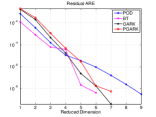
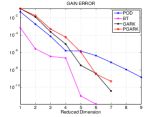
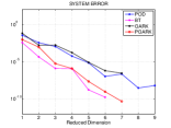
Figure 1: Test 1: Convergence history of the relative residual norm ${\tt R}_{P}$ (left), Error ${\mathcal{E}}_{K}$ of the feedback gain matrix (middle), Error $\mathcal{E}_{G}$ for the approximation of reduced transfer function (right)

In the middle panel of Figure 1, we show how well the feedback gain matrix $K$ can be approximated with order reduction methods. It is interesting to see how the basis functions computed by gark and pgark are able to approximate the matrix $K$ very well.

Finally, we would like to show the quality of the computed basis functions in the approximation of the dynamical system in the right panel of Figure 1. In this example, bt approximates the transfer function very well but this method requires the full accurate solution of two Lyapunov equations to be able to generate the reduced transfer function. In the large scale case this is clearly unfeasible.

Last remark goes to the iterative methods gark and pgark. We showed that, although the basis functions are built upon information of the ARE, they are also able to approximate the dynamical systems and the feedback gain matrix. This is a crucial point that motivates us to further investigate these methods in the context of the LQR problem. Furthermore, they are absolute feasible when the dimension $n$ of the dynamical system increases as shown in the left panel of Figure 2. We computed the CPU time of the iterative methods varying $\Delta x=\{0.1,0.05,0.025,0.0125,0,00625\}$. We note that both methods reach the desired accuracy in a few seconds even for $n=O(10^{4})$. On the contrary both pod and bt would be way more expensive since their cost heavily depends on the original dimension of the problem $n$. The right panel of Figure 2 reports the history of the relative residual norm as the iterations proceed.

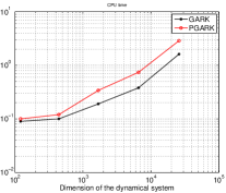
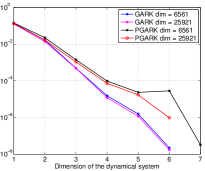
Figure 2: Test 1: Comparison of gark and pgark. Left: CPU time as the problem dimension $n$ increases. Right: relative residual norm history.

5.2 Test 2: 2D Linear Convection-Diffusion Equation

We consider the linear convection-diffusion equation in (14) with $\gamma=50,\varepsilon=1,\Omega=[0,2]\times[0,2]\mbox{ and }\Omega_{B}=[0.2,0.8]\times[0.2,0.8].$ In (1), the matrix $A$ is given by centered five points finite difference discretization plus an upwind approximation of the convection term (see e.g. Q12 ). The spatial discretization step is $\Delta x=0.1$ and leads to a system of dimension $n=441$. The matrix $C$ in (1) is given by the indicator function over the domain $\Omega_{C}=[0.1,0.9]\times[0.1,0.9],$ and $R\equiv I_{m}$ in (3).

The left panel of Figure 3 shows the residual norm history associated with the reduced ARE (7), with different projection techniques. We note that all the methods converge with a different number of basis functions. We also note that in this example we can observe instability of the pgark method as discussed in Section 4.1.

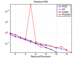
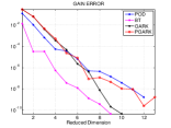
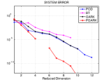
Figure 3: Test 2: History of the relative residual norm (left), Error $\mathcal{E}_{K}$ of the feedback gain matrix (middle), Transfer function error $\mathcal{E}_{G}$ as the approximation space grows (right)

Middle panel of Figure 3 reports the error in the approximation of the feedback gain matrix $K$. It is very interesting to observe that even on this convection dominated problem all the methods can reach an accuracy of order $10^{-8}$.

Finally, we show the error in the approximation of the transfer function in the right panel of Figure 3. In this example, we can see that the pgark method performs better than the others but it is rather unstable; this well known instability problem will be analyzed in future work.The discussion upon the quality of the basis function we had in Test 1 still hold true. The iterative methods are definitely a feasible alternative to well-known techniques as bt and pod.

In the left panel of Figure 4, we show the CPU time of gark and pgark for different dimensions $n$ of the dynamical systems. We note that, again, the Galerkin projection reaches the desired accuracy faster. The right panel of Figure 4 reports the history of the residual for both iterative methods, for two different values of $n$.

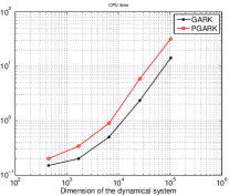
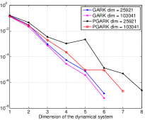
Figure 4: Test 2: Comparison of gark and pgark. Left: CPU time as the problem dimension $n$ increases. Right: relative residual norm history.

6 Conclusions

We have proposed a comparison of different model order reduction techniques for the ARE. We distinguished between two different strategies: (i) First reduction of the dynamical system complexity and then the solution of the corresponding reduced ARE whereas; (ii) Simultaneous solution of the ARE and determination of the reduction spaces. The strength of the second strategy is its reliability even for very high dimensional problem, where problems in the class (i) may have memory and computational difficulties. Experiments on both small and large dimensional problems confirm the promisingly good approximation properties of rational Krylov methods as compared to more standard approaches for the approximation of more challenging quantities in the LQR context.

References

- (1) A. Alla, M. Falcone, and S. Volkwein, Error analysis for POD approximations of infinite horizon problems via the dynamic programming approach, SIAM Journal on Control and Optimization, 55 (2017), pp. 3091–3115.
- (2) A. Alla, C. Graessle, and M. Hinze, A posteriori snapshot location for pod in optimal control of linear parabolic equations, submitted, https://arxiv.org/abs/1608.08665, (2016).
- (3) A. Alla and J. Kutz, Randomized model order reduction, submitted, https://arxiv.org/pdf/1611.02316.pdf, (2017).
- (4) A. Alla, A. Schmidt, and B. Haasdonk, Model order reduction approaches for infinite horizon optimal control problems via the hjb equation, in Model Reduction of Parametrized Systems, P. Benner, M. Ohlberger, A. Patera, G. Rozza, and K. Urban, eds., Springer International Publishing, Cham, 2017, pp. 333–347.
- (5) A. Antoulas, Approximation of Large–Scale Dynamical Systems, SIAM Publications, Philadelphia, PA, 2005.
- (6) J. Atwell and B. King, Proper orthogonal decomposition for reduced basis feedback controllers for parabolic equations, Mathematical and Computer Modelling, 33 (2001), pp. 1–19.
- (7) H. Barkouki, A. H. Bentbib, and K. Jbilou, An adaptive rational methodLanczos-type algorithm for model reduction of large scale dynamical systems, Journal of Scientific Computing, 67 (2015), p. 221–236.
- (8) C. Beattie and S. Gugercin, Model reduction by rational interpolation, in Model Reduction and Approximation: Theory and Algorithms, SIAM, Philadelphia, 2017.
- (9) P. Benner and Z. Bujanović, On the solution of large-scale algebraic Riccati equations by using low-dimensional invariant subspaces, Linear Algebra and Its Applications, 488 (2016), pp. 430–459.
- (10) P. Benner, A. Cohen, M. Ohlberger, and K. Willcox, eds., Model reduction and approximation: theory and Algorithms, Computational Science & Engineering, SIAM, PA, 2017.
- (11) P. Benner, J.-R. Li, and T. Penzl, Numerical solution of large-scale Lyapunov equations, Riccati equations, and linear-quadratic optimal control problems, Num. Lin. Alg. with Appl., 15 (2008), pp. 1–23.
- (12) P. Benner and J. Saak, A Galerkin-Newton-ADI method for solving large-scale algebraic Riccati equations., Tech. Rep. 1253, DF Priority program, 2010.
- (13) P. Benner and J. Saak, Numerical solution of large and sparse continuous time algebraic matrix Riccati and Lyapunov equations: A state of the art survey, GAMM-Mitt., (2013), pp. 32–52.
- (14) J. Borggaard and S. Gugercin, Model reduction for DAEs with an application to flow control, Active Flow and Combustion Control 2014, R. King editors, Springer-Verlag, Notes on Numerical Fluid Mechanics and Multidisciplinary Design,, 127 (2015), pp. 381–396.
- (15) V. Druskin and V. Simoncini, Adaptive rational Krylov subspaces for large-scale dynamical systems, Systems and Control Letters, 60 (2011), pp. 546–560.
- (16) M. Falcone and R. Ferretti, Semi-Lagrangian Approximation Schemes for Linear and Hamilton-Jacobi equations, SIAM, 2014.
- (17) L. Grüne and J. Pannek, Nonlinear model predictive control. Theory and algorithms, Springer Verlag, 2011.
- (18) S. Gugercin, A. C. Antoulas, and C. Beattie, model reduction for large-scale linear dynamical systems, SIAM J. Matrix Anal. Appl., 30 (2008), pp. 609–638.
- (19) M. H. Gutknecht, A completed theory of the unsymmetric Lanczos process and related algorithms. I, SIAM J. Matrix Anal. Appl., 13 (Apr. 1992), pp. 594–639.
- (20) M. Heyouni and K. Jbilou, An extended Block Krylov method for large-scale continuous-time algebraic Riccati equations, ETNA, 33 (2008-2009), pp. 53–62.
- (21) M. Hinze, R. Pinnau, M. Ulbrich, and S. Ulbrich, Optimization with PDE Constraints. Mathematical Modelling: Theory and Applications, Springer Verlag, New York, 2009.
- (22) I. M. Jaimoukha and E. M. Kasenally, Oblique projection methods for large scale model reduction, SIAM J. Matrix Anal. Appl., 16 (1995), pp. 602–627.
- (23) I. M. Jaimoukha and E. M. Kasenally, Krylov subspace methods for solving large Lyapunov equations, SIAM J. Numer. Anal., 31 (Feb. 1994), pp. 227–251.
- (24) K. Jbilou, Block Krylov subspace methods for large algebraic Riccati equations, Numerical Algorithms, 34 (2003), pp. 339–353.
- (25) D. Kleinman, On an iterative technique for riccati equation computations, IEEE Trans. Automat. Control, 13 (1968), pp. 114–115.
- (26) B. Kramer and J. Singler, A pod projection method for large-scale algebraic riccati equations., Numer. Algebra Control Optim., 4 (2016), pp. 413–435.
- (27) K. Kunisch and S. Volkwein, Proper orthogonal decomposition for optimality systems, ESAIM: Mathemematical Modelling and Numerical Analysis, 42 (2008), pp. 1–23.
- (28) P. Lancaster and L. Rodman, Algebraic Riccati equations, Oxford Univ. Press, 1995.
- (29) Y. Lin and V. Simoncini, Minimal residual methods for large scale Lyapunov equations, tech. rep., Dipartimento di Matematica, Università di Bologna, 2012.
- (30) Y. Lin and V. Simoncini, A new subspace iteration method for the algebraic Riccati equation, Numerical Linear Algebra w/Appl., 22 (2015), pp. 26–47.
- (31) A. Quarteroni, Modellistica numerica per problemi differenziali, Springer, 2012.
- (32) A. Schmidt and B. Haasdonk, Reduced basis approximation of large scale parametric algebraic Riccati equations, ESAIM: Control, Optimisation and Calculus of Variations, (2017).
- (33) V. Simoncini, Analysis of the rational Krylov subspace projection method for large-scale algebraic Riccati equations, SIAM J. Matrix Anal. Appl., 37 (2016), pp. 1655–1674.
- (34) , On the extended Krylov subspace method for the algebraic Riccati equation, January 2016. In preparation.
- (35) V. Simoncini, D. B. Szyld, and M. Monslave, On two numerical methods for the solution of large-scale algebraic riccati equations, IMA, J. Numer. Anal., 34 (2014), pp. 904–920.
- (36) L. Sirovich, Turbulence and the dynamics of coherent structures. parts i-ii, Quarterly of Applied Mathematics,, XVL (1987), pp. 561–590.
- (37) S. Volkwein, Model Reduction using Proper Orthogonal Decomposition, Lecture notes, University of Konstanz, 2011.