Abstract

An anisotropic measurement of the baryon acoustic oscillation (BAO) feature fixes the product of the Hubble constant and the acoustic scale $H_{0}r_{d}$. Therefore, regardless of the dark energy dynamics, to accommodate a higher value of $H_{0}$ one needs a lower $r_{d}$ and so necessarily a modification of early time cosmology. One must either reduce the age of the Universe at the drag epoch or else the speed of sound in the primordial plasma. The first can be achieved, for example, with dark radiation or very early dark energy, automatically preserving the angular size of the acoustic scale in the Cosmic Microwave Background (CMB) with no modifications to post-recombination dark energy. However it is known that the simplest such modifications fall afoul of CMB constraints at higher multipoles. As an example, we combine anisotropic BAO with geometric measurements from strong lensing time delays from H0LiCOW and megamasers from the Megamaser Cosmology Project to measure $r_{d}$, with and without the local distance ladder measurement of $H_{0}$. We find that the best fit value of $r_{d}$ is indeed quite insensitive to the dark energy model, and is also hardly affected by the inclusion of the local distance ladder data.

1 Introduction

1.1 Motivation

The $\Lambda$CDM cosmological model has become the Standard Model of cosmology in the past 20 years in part because its remarkably simple treatment of cosmological acceleration [1, 2, 3], as the result of a cosmological constant, has been confirmed time and time again with ever greater precision and at various redshifts by multiple cosmological probes. On the other hand, through its consistency with various cosmological properties, while remaining in a regime which is generally believed to allow a semiclassical treatment (but see Ref. [4]), the inflationary paradigm has won the hearts of most cosmologists and so has been effectively incorporated into this Standard Cosmological Model. Inflation also comes with cosmological acceleration, but the origin is the condensate of a new field, the inflaton, and not a cosmological constant. Although the inflaton has never been observed, many other such condensates are known to exist in the electroweak and strongly interacting sectors of the Standard Model of particle physics. The fact that known condensates do not yield acceleration, as would be expected by minimally coupling gravity to the Standard Model, is usually attributed to an unknown mechanism which somehow does not prevent the inflaton from causing acceleration.

Despite these theoretical gaps, a consistent picture has emerged. The Universe is accelerating now and this acceleration is well described by a cosmological constant, which fits the expansion data extraordinarily well at $z<1$, and it also underwent many efolds of acceleration at very high redshift. Given these bouts of expansion at early and late times, one may wonder about acceleration in the middle [5]. Clearly efolds of intermediate time acceleration are observationally excluded, but in the age of precision cosmology even a few percent of anomalous expansion, which could be called early dark energy whether before or after recombination, could skew parameter measurements beyond their reported uncertainties and lead to tension between various datasets. Ref. [6] has shown that one such model can lead to a shift of the best fit $H_{0}$ of 1.6 km/sec/Mpc with no other deviations from $\Lambda$CDM invoked, while some older models satisfy looser bounds [7].

Early dark energy is just one of many examples of new physics which would affect the cosmological expansion rate. While some parametrizations of interactions between dark energy and dark [8, 9] or even visible matter [10] or dark energy itself [11] have been studied, in general dark matter may also simply decay to radiation with a lifetime of order $10^{11}$ years, which would cause a deficit in the dark matter today as compared with that at, say $z>1$ as well as nonneglible dark radiation today. On the other hand, in solitonic dark matter models, dark matter is nucleated, for example via the Kibble mechanism, and so dark energy (gravitating or not) is turned into dark matter before recombination [12, 13]. Similarly in Bose Einstein Condensate dark matter models [14, 15], the dark matter condenses at some early time. These models predict a dark matter surplus at recent times as compared with that before recombination, as does the interacting dark matter-dark energy model of Ref. [16] when fit to recent cosmological datasets.

The cosmological Standard Model, like the Standard Model of particle physics and that of neutrino physics, has its 2$\sigma$ and 3$\sigma$ anomalies. History shows that most of these anomalies disappear [17], nonetheless some may lead the way beyond $\Lambda$CDM and so their study is a central topic in each field. The upshot of the above meandering discussion is that it is hopeless to parameterize all of the possible deviations from $\Lambda$CDM and conversely, given a short list of favored deviations from $\Lambda$CDM it is unlikely that the resolution to a given anomaly will lie on the list.

1.2 Methodology

This motivates studies of these anomalies which are as model-independent as possible. Therefore we will restrict our attention to geometric observables, which are less prone to some systematics arising from stellar evolution and dust extinction, although in general they are affected by modelling assumptions. In particular, following the logic of Ref. [20] we will assume only homogeneity, isotropy, minimal coupling of electromagnetism to gravity (so that light follows geodesics) and that the BAO length scale $r_{d}$ is position independent in comoving coordinates to determine $r_{d}H(z)$ and weighted combinations thereof from anisotropic BAO measurements.

Were $H(z)$ known directly, one could immediately determine $r_{d}$. This is not the case. Instead we will use the weighted combination of $H(z)$ values which appears in the strong lensing time delay distances determined by the H0LiCOW collaboration. These will be combined with the angular diameter distances to masers from the Megamaser Cosmology Project, which largely constrain $H_{0}$. To bind these disparate measurements of combinations of $H(z)$’s together, we will assume that the evolution of the dark energy density is sufficiently smooth to be well approximated at these low redshifts by various simple parameterizations such as the linear CPL form [21, 22].

This assumption may appear to be in contradiction with the preceding diatribe on the needed generality in a study of dark energy, but actually this assumption is only imposed at the redshifts of the data considered. In particular, at $z>1$ only one set of anisotropic BAO data is used, and it has a small effect on the best fits, and so this assumption essentially only constrains the dark energy behavior at $z<1$ where any gross violation would likely be apparent in 1a supernova Hubble diagrams. Therefore our results would be minimally affected by any change in the dark energy dynamics at $z>1$ and would be entirely unaffected by any dark energy dynamics at $z>2.4$.

We will then use a straightforward frequentist likelihood analysis to combine these measurements into profile likelihoods for $r_{d}$, with nuisance parameters chosen to maximize the likelihood function. The resulting value will be between 135 and about 140 Mpc depending in the data set and dark energy model. This is somewhat lower than the best fit Planck results [23] in the case of a $\Lambda$CDM cosmology, which we adopt as a benchmark. We find that our best fit value is somewhat robust against changes in the dark energy model, and even changes in the dataset so long as BAO is included. However we find that the inclusion of the local distance ladder measurement of $H_{0}$ from Ref. [24], as has been done in Ref. [25], reduces the uncertainty in $r_{d}$ and so increases the statistical significance of this incompatibility.

The evidence for a model which is qualitatively similar to $\Lambda$CDM is quite overwhelming, and so we will argue that the redshift to the drag epoch at which $r_{d}$ measures the acoustic length scale is robust at the level of precision of these likelihoods. Therefore the low $z$ measurements determine the metric size of the acoustic feature at the drag epoch and find it to be smaller than the benchmark Planck value.

These Planck results assume a $\Lambda$CDM model and we do not investigate how a change in the dark energy model would affect the Planck best fit, a task which we leave to the sequel. This is because our goal in the present paper is not to test the analysis of Planck data nor to fit the CMB data to our models, but rather to use probes of late time cosmology to learn about $r_{d}$. CMB measurements, being sensitive directly to a number of features of early time cosmology, are not suitable for this task. The role of the the Planck $\Lambda$CDM best fit in this paper is simply as a benchmark: As the Planck best fit value is widely used for a number of cosmological and astrophysical applications, we feel that it is useful to test it against various cosmological datasets and models even if the models are not those from which this Planck best fit is derived. Perhaps more to the point, there are many ways in which a smaller $r_{d}$ could be achieved by modifying early Universe cosmology. These are equivalent from the point of view of our late time geometric probes, however they affect the CMB differently. Therefore a study of their effects on the CMB would need to consider many rather different cases, and even so is unlikely to be exhaustive.

If the best fit value of $r_{d}$ derived here from BAO, lensing and megamaser data is to be realized in Nature, then one requires a change in early time cosmology. In particular the change in early time cosmology must either reduce the age of the Universe at recombination or else it must reduce the speed of sound of the primordial plasma. This explains the observation in Refs. [28, 29] that, while modifications in the dark energy equation of state may reconcile tension between CMB and local distance ladder measurements, no such change to late time cosmology removes the tension when BAO is included, a result that has been extended to late time dark matter-dark energy interactions in Ref. [30]. This situation is in contrast with the tension between the BAO Lyman $\alpha$ forest and galaxy clustering datasets, which lies entirely in the late time expansion of the Universe [31] and need not affect, for example, the angular diameter distance to recombination.

This of course will beg the question of just what modifications would be consistent with the CMB data. The line of argument of the current paper is deductive and quite model independent: from certain assumptions and given certain data we establish necessary and sufficient conditions for consistency with BAO, strong lensing and megamaser data. However, given the wealth of modifications to early time cosmology that satisfy this criteria, we know of no such model independent conclusions regarding the CMB and so will only make some general remarks considering specific CMB constraints and will leave model-building to the sequel.

2 Data

2.1 BAO Data

We combine isotropic BAO measurements from the 6dF Survey [32], at an effective redshift of $z=0.106$, with the reconstructed Sloan Digital Sky Survey Data Release 7 [33] main galaxy sample (MGS) at an effective redshift of $z=0.15$ and the extended Baryon Oscillation Spectroscopic Survey (eBOSS) quasar clustering at $z=1.52$ [34] with the anisotropic measurements from the BAO only analysis of the Baryon Oscillation Spectroscopic Survey (BOSS) analysis [35] and Lyman $\alpha$ forest samples [36] at effective redshifts of $z=0.38$, $z=0.51$, $z=0.61$ and $z=2.4$.

Data Set	Redshift	Constraint	Ref.
6dF	$z=0.106$	$\frac{D_{V}(0.106)}{r_{d}}=2.98\pm 0.13$	[32]
MGS	$z=0.15$	$\frac{D_{V}(0.15)}{r_{d}}=4.47\pm 0.17$	[33]
eBOSS quasars	$z=1.52$	$\frac{D_{V}(1.52)}{r_{d}}=26.1\pm 1.1$	[34]

Table 1: Isotropic BAO scale measurements used in this analysis.

Data Set	Redshift	Constraint	Ref.
BOSS DR12	$z=0.38$	$\frac{D_{A}(0.38)}{r_{d}}=7.42$	[35]
BOSS DR12	$z=0.38$	$\frac{D_{H}(0.38)}{r_{d}}=24.97$	[35]
BOSS DR12	$z=0.51$	$\frac{D_{A}(0.51)}{r_{d}}=8.85$	[35]
BOSS DR12	$z=0.51$	$\frac{D_{H}(0.51)}{r_{d}}=22.31$	[35]
BOSS DR12	$z=0.61$	$\frac{D_{A}(0.61)}{r_{d}}=9.69$	[35]
BOSS DR12	$z=0.61$	$\frac{D_{H}(0.61)}{r_{d}}=20.49$	[35]
BOSS DR12	$z=2.4$	$\frac{D_{A}(2.4)}{r_{d}}=10.76$	[36]
BOSS DR12	$z=2.4$	$\frac{D_{H}(2.4)}{r_{d}}=8.94$	[36]

Table 2: Anisotropic BAO scale measurements used in this analysis.

The isotropic and anisotropic BAO measurements are summarized in Tables 1 and 2 respectively. The BAO only analysis of Ref. [35] is used, which only uses the peak location and not the matter power spectrum shape. The uncertainties for this analysis were not reported in that reference but are available from the SDSS website in the file BAO_consensus_covtot_dM_Hz.txt. Combined with the covariance matrix for the Lyman $\alpha$ BAO detection in Ref. [36], the covariance matrix corresponding to the data in Table 2 is

$${\mathbf{C}}=\left(\begin{tabular}[]{cccccccc}0.0150&-0.0358&0.0071&-0.0100&0.0032&-0.0036&0&0\\ -0.0357&0.5304&-0.0160&0.1766&-0.0083&0.0616&0&0\\ 0.0071&-0.0160&0.0182&-0.0323&0.0097&-0.0131&0&0\\ -0.0100&0.1766&-0.0323&0.3267&-0.0167&0.1450&0&0\\ 0.0032&-0.0083&0.0097&-0.0167&0.0243&-0.0352&0&0\\ -0.0036&0.0616&-0.0131&0.1450&-0.0352&0.2684&0&0\\ 0&0&0&0&0&0&0.1358&-0.0296\\ 0&0&0&0&0&0&-0.0296&0.0492\\ \end{tabular}\right).$$ (2.1)

This data is combined into a $\chi^{2}$ statistic

$$\chi^{2}_{\rm{BAO}}=\chi^{2}_{\rm{iso}}+\chi^{2}_{\rm{aniso}},\hskip 11.38092pt\chi^{2}_{\rm{iso}}=\sum_{i}\left(\frac{v_{i}-d^{\rm{iso}}_{i}}{\sigma_{i}}\right)^{2},\hskip 11.38092pt\chi^{2}_{\rm{aniso}}=\left(\mathbf{w-d}^{\rm{aniso}}\right)^{\perp}\mathbf{C}^{-1}\left(\mathbf{w-d}^{\rm{aniso}}\right)$$ (2.2)

where the vectors $\mathbf{d}^{\rm{iso}}$ and $\mathbf{d}^{\rm{aniso}}$ are the isotropic and anisotropic best fit data from Tables 1 and 2 and $\mathbf{v}$ and $\mathbf{w}$ are the predictions for these vectors in a given cosmological model. The $\sigma_{i}$ are the uncertainties from Table 1. Due to the relatively small number of mocks, the Lyman $\alpha$ forest BAO likelihood profile deviates noticeably from the Gaussian form used here when a model is more than about 2$\sigma$ from the data. However this dataset will contribute to our fits essentially only by shifting the best fit parameters for the dark energy evolution, and once this shift has occurred the model will lie within 2$\sigma$ of the data, and so this non-Gaussianity is inconsequential for our study of $H_{0}$. It would be relevant if we were searching for evidence for dark energy dynamics or if we used the likelihoods of the dark energy parameters far from their maxima.

2.2 Other Data

The BAO data does not directly constrain $r_{d}$, $H_{0}$ or even $H(z)$, rather it constrains various weighted averages of $H(z)r_{d}$. Our goal is to use low redshift observations to measure $r_{d}$, therefore we need independent constraints on $H(z)$. There are a number of cosmological probes which are sensitive to $H(z)$ (for example the cosmic chronometers of Ref. [37]). We will largely restrict our attention to geometric probes, which determine $H(z)$ using geometry, as these are independent of many of the astrophysical and cosmological assumptions that may affect the others. For example, they are not affected by stellar evolution, dust extinction or variations in local metalliticity. Most importantly for our analysis, they are reasonably robust, as compared with the present uncertainties, against changes in the cosmological model at higher redhshifts than the observations themselves.

There remain of course some sources of systematic error which are difficult to quantify, in particular regarding modelling. For example, in the case of the Lyman $\alpha$ BAO analysis, one needs to estimate the continuum component of the Lyman $\alpha$ absorption, so that it may be subtracted to obtain the forest and extract the corresponding mass density. In the near future eBOSS will complete its anisotropic BAO analysis of the quasar-quasar correlation function at similar redshfits [38] allowing an independent test of these BAO measurements.

In the case of strong lensing time delays, the determination of the time delay distance requires a determination of the density profile of the lens and the line of sight [39], but there are several potentially dangerous degeneracies in the construction of the lens model [40, 41] from the observed source positions. To break these degeneracies in the determination of the lens profile, one generally uses the line of sight velocity dispersion. However, given the line of sight velocity dispersion there is an exact degeneracy between the density profile and the unknown velocity anisotropy [42]. In principle, without a measurement of the velocity anisotropy, which is infeasible at cosmological distances, the density profile cannot be constrained and thus the cosmological parameter estimates may be biased [43, 44]. The H0LiCOW collaboration treats this problem in Ref. [45] by assuming that the velocity anisotropy has a certain functional dependence on the radius, with one free parameter, and then that parameter is marginalized using a uniform prior with a fixed range. Needless to say, both the choice of parameterization and the prior on the parameter are assumptions, leading to contributions to the error budget which are difficult to quantify. In the future, some improvement will come from spatially resolved kinematics [46].

This problem will be ameliorated in the era of extremely large telescopes, which will provide both high resolution images of these lens systems [47] and also proper motion measurements of stars in galaxies of various morphologies as far as the Virgo cluster. One can then motivate an anisotropy profile for the lens system by comparing it to similar, nearby systems whose anisotropies have been measured.

To determine the mass distribution along the line of sight, Ref. [48] uses such mass distributions in $\Lambda$CDM simulations. This will eventually limit the applicability of high precision strong lensing time delays to cosmologies which are sufficiently similar to the fiducial cosmologies of the simulations.

In the case of water megamasers, modelling the maser itself is essential. For example. if the number of rings is determined incorrectly, or if part of the signal is interpreted as arising from the wrong ring, this would lead to an error which is unlikely to be quantified by the assigned error budget. This is a problem that in principle can be solved with deeper, higher resolution images.

Lens	$z_{d}$	$z_{s}$	$\mu_{d}$	$\sigma_{D}$	$\lambda_{D}$	Ref.
B1608+656	$0.6304$	$1.394$	$7.0531$	$0.22824$	$4000.0$	[51]
RXJ1131-1231	$0.295$	$0.654$	$6.4682$	$0.20560$	$1388.8$	[52]
HE0435-1223	$0.4546$	$1.693$	$7.5793$	$0.10312$	$653.9$	[45]

Table 3: Strong lensing time delays used in this analysis.

The main dataset which we will use is the collection of strong lensing time delays produced by the H0LiCOW collaboration. This program is described in Ref. [49] and the data is summarised in Table 3 of Ref. [50] and is repeated in Table 3 of the present note. Here $z_{s}$ and $z_{d}$ are the redshift of the source quasar and the lensing galaxy respectively. The parameters $\lambda_{D}$, $\mu_{D}$ and $\sigma_{D}$ determine the likelihood of a given time delay distance $D_{\Delta t}=x$ as

$$P(x)=\frac{1}{\sqrt{2\pi}\left(x-\lambda_{D}\right)\sigma_{D}}\rm{exp}\left[-\frac{\left({\rm{ln}}\left(x-\lambda_{D}\right)-\mu_{D}\right)^{2}}{2\sigma_{D}^{2}}\right].$$ (2.3)

By an abuse of notation we will simply refer to $-2$ times the log likelihood as $\chi^{2}_{\rm{lens}}$

$$\chi^{2}_{\rm{lens}}=-2\ {\rm{ln}}(P(x))=\frac{\left({\rm{ln}}\left(x-\lambda_{D}\right)-\mu_{D}\right)^{2}}{\sigma_{D}^{2}}+2\ {\rm{ln}}\left[\sqrt{2\pi}\left(x-\lambda_{D}\right)\sigma_{D}\right].$$ (2.4)

We will also use angular diameter distances measured using water megamasers under the Megamaser Cosmology Project [53]. We do not include the uncertainty in the distance caused by the peculiar velocity, as this has a negligible effect on our results. The data are summarized in Table 4. The $\chi^{2}$ statistic $\chi^{2}_{\rm{maser}}$ will be calculated using the same standard formula as is used for $\chi^{2}_{\rm{iso}}$ in Eq. (2.2). We will not use the megamaser NGC 6323 [57] or the Hubble parameter determination from the standard siren GW170817 [58, 59] because, due to their large uncertainties, they would have a negligible effect on our results. We note that these standard siren measurements are not purely geometric in that it is assumed that the source galaxy has been correctly identified and, more importantly, a 10% correction to the recessional velocity is applied to correct for the peculiar velocity caused by the local gravitational field. In addition the latter reference uses an estimate of the inclination angle based on a model of the system’s jet.

Maser	Redshift	Constraint	Ref.
UGC 3789	$z=0.0116$	$\frac{D_{A}(0.0116)}{\rm{Mpc}}=49.6\pm 5.1$	[54]
NGC 6264	$z=0.0340$	$\frac{D_{A}(0.0340)}{\rm{Mpc}}=144\pm 19$	[55]
NGC 5765b	$z=0.0277$	$\frac{D_{A}(0.0277)}{\rm{Mpc}}=126.3\pm 11.6$	[56]

Table 4: Megamaser measurements used in this analysis.

Finally, we will sometimes include the distance ladder measurement $H_{0}=73.24\pm 1.74$ km/sec/Mpc from Ref. [24]. It is not an entirely geometric measurement, even if it uses megamasers in part, however it relies upon astrophysical instead of cosmological assumptions and is independent of early time cosmology.

3 Results

3.1 Models

Cosmology	Parameters	Constraints
$\Lambda$CDM-Planck	$r_{d}$	$\Omega_{m}=0.31,\ P=30.0,\ w(z)=-1$
H$\Lambda$CDM-Planck	$r_{d},\ H_{0}$	$\Omega_{m}=0.31,w(z)=-1$
$\Lambda$CDM	$r_{d},\ \Omega_{m},\ H_{0}$	$w(z)=-1$
$w$CDM	$r_{d},\ \Omega_{m},\ H_{0},\ w$	$w(z)=w$
CPL	$r_{d},\ \Omega_{m},\ H_{0},\ w_{0},\ w_{a}$	$w(z)=w_{0}+\frac{z}{1+z}w_{a}$

Table 5: Five cosmological models

We consider the five cosmological models summarized in Table 5. The first is the standard, flat $\Lambda$CDM cosmology with the parameters $\Omega_{m}$ and

$$P=\frac{c}{H_{0}r_{d}}$$ (3.1)

fixed to their best fit values from the Planck experiment [23] including lensing and polarization data. Note however that we do not fix $r_{d}$, since our goal is to determine a likelihood for $r_{d}$. In the second, $H_{0}$ is freed. The third is also a flat $\Lambda$CDM model with dark energy equation of state $w(z)=-1$, but $r_{d}$, $P$ and $\Omega_{m}$ unconstrained. Next, we consider the same model but allow the dark energy equation of state $w(z)$ to assume any $z$-independent value $w$. Finally, we consider a flat cosmology with $w(z)$ of the CPL form [21, 22]

$$w(z)=w_{0}+\frac{z}{1+z}w_{a}.$$ (3.2)

3.2 Analysis

In a spatially flat Universe with electromagnetism minimally coupled to gravity, the various cosmological distances described above can be written

$$D_{A}(z) = \frac{c}{1+z}\int_{0}^{z}\frac{dz^{\prime}}{H(z^{\prime})}$$ (3.3)

$$D_{H}(z) = \frac{c}{H(z)}$$

$$D_{V}(z) = \left((1+z)D_{A}(z)\right)^{2/3}\left(zD_{H}(z)\right)^{1/3}$$

$$D_{\Delta t}(z_{d},z_{s}) = c\frac{\int_{0}^{z_{d}}\frac{dz^{\prime}}{H(z^{\prime})}\int_{0}^{z_{s}}\frac{dz^{\prime}}{H(z^{\prime})}}{\int_{z_{d}}^{z_{s}}\frac{dz^{\prime}}{H(z^{\prime})}}$$

where $c$ is the speed of light and the function $H(z)$ is given by

$$H(z)=H_{0}\sqrt{\Omega_{m}(1+z)^{3}+(1-\Omega_{m})e^{3\int_{0}^{z}\frac{1+w(z^{\prime})}{1+z^{\prime}}dz^{\prime}}}$$ (3.4)

in terms of the Hubble parameter $H_{0}$, the matter fraction of the critical density $\Omega_{m}$ and the equation of state of dark energy $w(z)$. Using these formulas, for a given cosmological model in Table 5 one can find the observables (3.3) and so can calculate the $\chi^{2}$ functions and log likelihoods described in Sec. 2.

The above formula for $D_{\Delta t}(z_{d},z_{s})$ was derived from the usual formula in terms of angular diameter distances

$$D_{\Delta t}(z_{d},z_{s})=(1+z_{d})\frac{D_{d}D_{s}}{D_{ds}}$$ (3.5)

using the identities

$$D_{s}=\frac{c}{1+z_{s}}\int_{0}^{z_{s}}\frac{dz^{\prime}}{H(z^{\prime})},\hskip 11.38092ptD_{d}=\frac{c}{1+z_{d}}\int_{0}^{z_{d}}\frac{dz^{\prime}}{H(z^{\prime})},\hskip 11.38092ptD_{ds}=\frac{c}{1+z_{s}}\int_{z_{d}}^{z_{s}}\frac{dz^{\prime}}{H(z^{\prime})}.$$ (3.6)

We are interested in the value of $r_{d}$ consistent with various datasets, since a modification of $r_{d}$ requires a modification of early time cosmology and we want to know whether early time cosmology indeed needs to be modified to accommodate current data, in contrast with claims in the literature [60]. However the models at hand contain a number of other parameters. In line with our desired level of model-independence, we do not wish to impose priors on these nuisance parameters. Therefore we will opt for a frequentist analysis.

We will use the profile likelihood, which has many of the same properties as the likelihood function itself [61], even if one allows the full set of functions $w(z)$ instead of parametrizing it [62] as is done here. The profile likelihood function is obtained by simply maximising the likelihoods of the nuisance parameters, or equivalently minimizing the values of $\chi^{2}$. More precisely, for each cosmological model, and each set of datasets, we will add the corresponding log likelihoods. Then for each value of $r_{d}$ we will choose all of the other parameters so as to maximize this sum. The result is the profile log likelihood for $r_{d}$. We will double this so that we get an estimator which is roughly speaking a $\chi^{2}$ statistic. We will report the quantity $\Delta\chi^{2}$, which is minus twice the profile log likelihood minus its own minimal value. We report this quantity because Wilks’ theorem guarantees that $\Delta\chi^{2}$ will nearly follow a $\chi^{2}$ distribution with one degree of freedom.

We also estimate the 1$\sigma$ uncertainty on $r_{d}$ as half of the size of the interval at which this $\Delta\chi^{2}$ is less than one. The corresponding interval is the range of values of $r_{d}$ for which there exists a set of nuisance parameters that yields a $p$ value greater than 0.32. Note that the nuisance parameters are optimized, not marginalized, in this analysis and so no priors are needed.

3.3 Results

BAO only

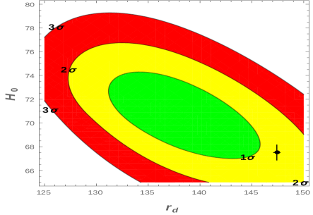
Using only the BAO data, one can determine $c/(H(z)r_{d})$ but it is not possible to separate $H(z)$ and $r_{d}$. Therefore there is no difference between the compatibility of the data with the $\Lambda$CDM-Planck and H$\Lambda$CDM-Planck models, as $r_{d}$ and $H_{0}$ are separately unconstrained. Given a dark energy model at the redshifts of the BAO data, one can choose the nuisance parameters to maximize the likelihood and so obtain the profile likelihood for $P=c/(H(z)r_{d})$ in that model. The simplest case is that of $\Lambda$CDM, where the only parameters which affect the likelihood are $P$ and $\Omega_{m}$.

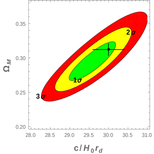
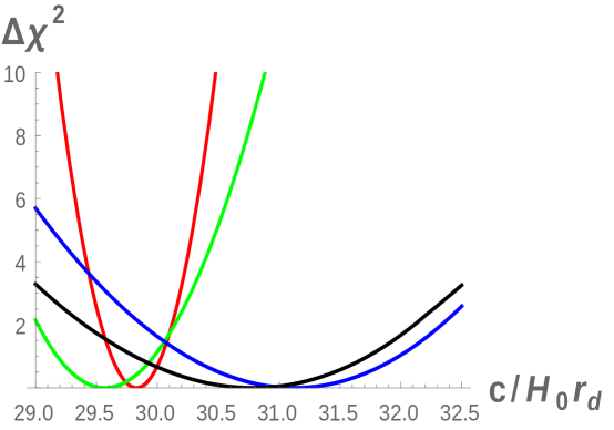
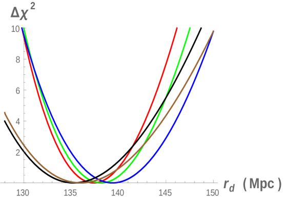
The full two-dimensional $\Delta\chi^{2}$ on this parameter space is depicted in the first panel of Fig. 1. The Planck $\Lambda$CDM best fit value [23] with its associated uncertainties is shown and excellent agreement can be seen. The profile likelihoods for $P$ are drawn in the second panel of Fig. 1 and the corresponding 1$\sigma$ uncertainties are reported in Table 6.

Figure 1: BAO only results. Top: In the $\Lambda$CDM model, the only relevant parameters are $\Omega_{m}$ and $c/(H_{0}r_{d})$. The standard error ellipses are plotted, corresponding to $\Delta\chi^{2}_{\rm{BAO}}=2.3,\ 6.0$ and $11.8$. The Planck benchmark value, with its corresponding error bars derived in the case of a $\Lambda$CDM model, is included for comparison. Bottom: $\Delta\chi^{2}$ is plotted for various values of $c/(H_{0}r_{d})$ with all nuisance parameters optimized. The red, green, blue and black curves correspond to the $H\Lambda$CDM-Planck, $\Lambda$CDM, wCDM and CPL models respectively.

BAO and strong lensing

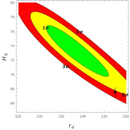
Next strong lensing time delays from H0LiCOW are included in the analysis. Each of the three strong lenses gives a time delay distance which constrains a combination of the $H(z)$. These are independent of $r_{d}$ and so $r_{d}$ and $H_{0}$ can now be separately determined. The corresponding log likelihood, denoted $\Delta\chi^{2}$, of $r_{d}$ and $H_{0}$ is shown in the first panel of Fig. 2 together with the Planck benchmark $H_{0}=67.51\pm 0.64$ and $r_{d}=147.41\pm 0.4$. One may observe a mild tension of about 2$\sigma$.

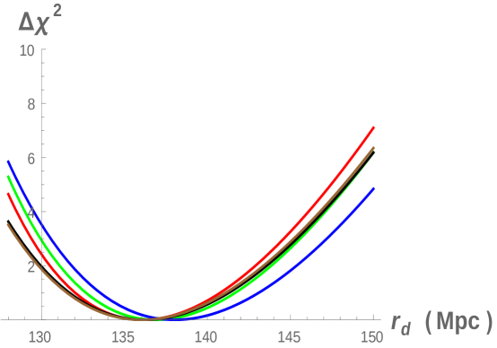
The second panel shows the profile log likelihoods of the various cosmological models, where all parameters except for $r_{d}$ are optimized. There is no sign that dynamical dark energy provides a better agreement with the benchmark value. On the contrary, the only model with less than 2$\sigma$ of tension is $\Lambda$CDM. The maximum likelihood value of $r_{d}$ is between 136 and 137 Mpc for all models except for $\Lambda$CDM, for which it is 138 Mpc. The corresponding 1$\sigma$ uncertainties are reported in Table 6. More general dark energy models have little effect on the uncertainty as these mostly affect the Lyman alpha BAO data, which in turn hardly influences the determination of $P$ and so $r_{d}$. One sees that in each case the maximum likelihood $r_{d}$ is roughly 2$\sigma$ below the Planck value.

Figure 2: BAO and strong lensing time delay results. Top: In the $\Lambda$CDM model, the only relevant parameters are $\Omega_{m}$, $r_{d}$ and $H_{0}$. The standard error ellipses are plotted with $\Omega_{m}$ optimized, $H_{0}$ in units of km/s/Mpc and $r_{d}$ in units of Mpc. Bottom: $\Delta\chi^{2}$ is plotted for various values of $H_{0}$ with all nuisance parameters optimized. The red, green, blue, black and brown curves correspond to the $\Lambda$CDM-Planck, H$\Lambda$CDM-Planck, $\Lambda$CDM, wCDM and CPL models respectively.

BAO, strong lensing and masers

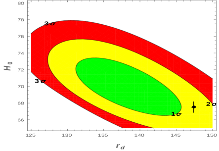
Masers are included in the analysis in Fig. 3. As can be seen there, and in Table. 6, the masers pull the best fit $r_{d}$ slightly towards the Planck value. Indeed the maser data is consistent with the Planck best fit values, but the uncertainties are so large that they only lead to an increase in $r_{d}$ of roughly one half of a standard deviation. Therefore at this point the mild tension lies entirely between the BAO value of $r_{d}H_{0}$, the Planck value of $r_{d}$ and the strong lensing time delay value of $H_{0}$.

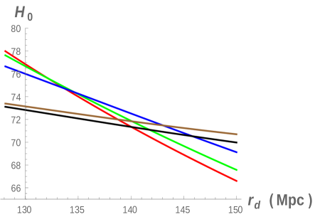
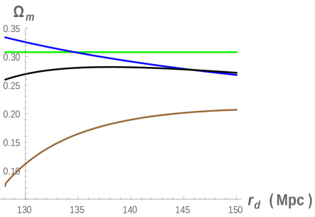
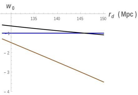
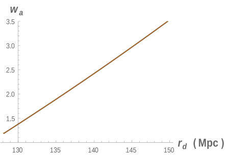
As this analysis is our main result, we also include the nuisance parameters which maximize the likelihood at each value of $r_{d}$. These are displayed in Fig. 4. While the CPL best fit dark energy dynamics is quite far from a cosmological constant, one can see in Table 6 that it leads to essentially identical confidence intervals for $r_{d}$. The role of the dynamical dark energy is largely just to satisfy the Lyman $\alpha$ BAO measurement. This is quite different from the case of Refs. [28, 29, 60] where the dynamical dark energy instead serves to change the angular diameter distance to recombination and thus to allow compatibility of the distance ladder $H_{0}$ with the Planck CMB $r_{d}$. The strong role of BAO in our study keeps the $r_{d}$ far from the Planck value and so no modification to this angular diameter distance is needed.

Figure 3: As in the bottom panel of Fig. 2, but also including megamaser data.

Figure 4: The profiled values of the nuisance parameters in the fit of BAO, lensing and maser data. The red, green, blue, black and brown curves correspond to the $\Lambda$CDM-Planck, H$\Lambda$CDM-Planck, $\Lambda$CDM, wCDM and CPL models respectively.

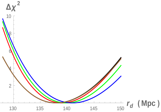
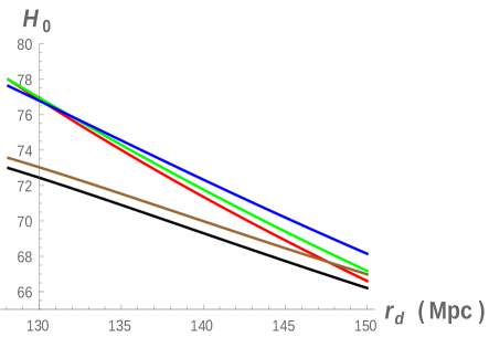
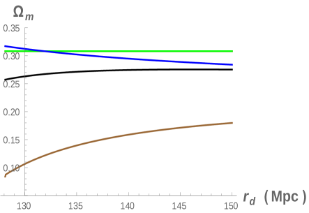
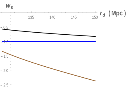
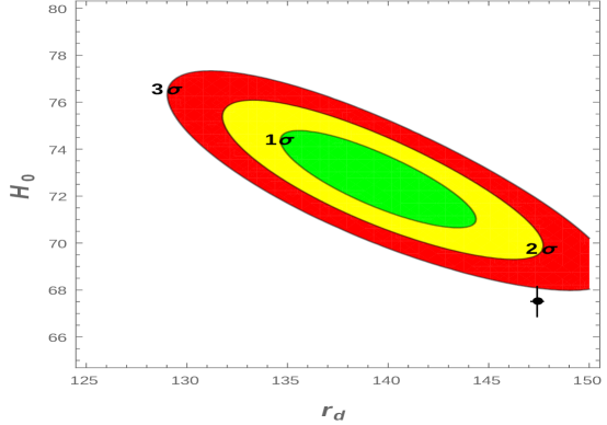
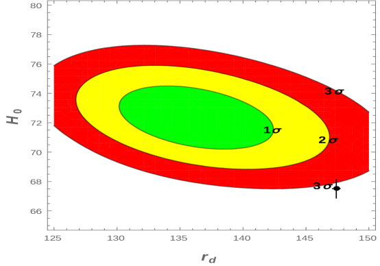
To further illustrate this point, in Fig. 5 we have plotted the two-dimensional profile log likelihoods of $r_{d}$ and $H_{0}$ in each cosmological model in which $H_{0}$ is free. One may observe that the level of compatibility of our best fit and the Planck $\Lambda$CDM benchmark hardly changes when dynamical dark energy is allowed. This is despite the fact that dynamical dark energy significantly thickens the minor axis of the standard error ellipse, reducing the strong correlation between $H_{0}$ and $r_{d}$. This is because while $r_{d}H_{0}$, the combination best constrained by BAO, is somewhat sensitive to the dark energy dynamics, the difference between the Planck $\Lambda$CDM best fit $(r_{d},\ H_{0})$ and the best fit here in fact lies along the least constrained direction (the semimajor axis), which appears entirely unaffected by the dark energy dynamics. The semimajor axis constraint results from the local measurements of the Hubble constraint using strong lensing and megamasers, which are fairly insensitive to dark energy dynamics due to their low redshifts.

Figure 5: The standard error ellipses corresponding to the profile likelihood for $H_{0}$ and $r_{d}$, with all nuisance parameters optimized. BAO, strong lensing and megamaser data are used. Top-left: H$\Lambda$CDM-Planck, Top-right: $\Lambda$CDM, Bottom-left: wCDM and Bottom-right: CPL model.

BAO, strong lensing, masers and the local distance ladder

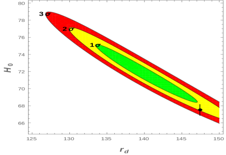
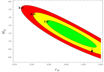
Finally the $H_{0}$ from the local distance ladder is included in Figs. 6 and 7. In Table 6 one can see that this inclusion in fact has a only a modest effect on the best fit value of $r_{d}$. This reflects the consistency between the local distance ladder and strong lensing time delay measurements of $H_{0}$. The reduction in the uncertainty is between 20% and 40%, depending on the model. The tension with the Planck $\Lambda$CDM benchmark values in each case remains about 3$\sigma$, increasing to 4$\sigma$ in the first two models, which incorporate some of the Planck $\Lambda$CDM parameter constraints.

Figure 6: As in the bottom panel of Fig. 2, but also including megamaser data and the local distance ladder determination of $H_{0}$.

In Fig. 8 we have plotted the two-dimensional profile log likelihoods of $r_{d}$ and $H_{0}$ in the $\Lambda$CDM and CPL models. Unlike Fig. 5, the tension is now greater than 3$\sigma$ in each case. However, as in that case, one observes that dynamical dark energy does not reduce the tension. Again dynamical dark energy thickens the minor axis of the error ellipse. However the strong constraint on $H_{0}$ means that this thickening is balanced by a rotation of the ellipse towards the horizontal direction, which prevents a reduction of the tension.

Figure 7: As in Fig. 4, but including the local distance ladder determination of $H_{0}$.

Figure 8: The standard error ellipses corresponding to the profile likelihood for $H_{0}$ and $r_{d}$, with all nuisance parameters optimized. BAO, strong lensing, megamasers and the local distance ladder are used. Top: $\Lambda$CDM, Bottom: CPL model.

Cosmology	BAO only	BAO$+$lensing	$+$masers	$+H_{0}$
$\Lambda$CDM-Planck	$29.8\pm 0.2$	$136.1\pm 4.7$	$139.0\pm 4.6$	$137.4\pm 2.6$
H$\Lambda$CDM-Planck	$29.8\pm 0.2$	$136.9\pm 4.8$	$139.8\pm 4.7$	$138.2\pm 2.8$
$\Lambda$CDM	$29.6\pm 0.4$	$138.0\pm 5.1$	$141.0\pm 4.6$	$139.4\pm 3.3$
$w$CDM	$31.1\pm 0.9$	$136.2\pm 5.1$	$137.9\pm 5.0$	$135.3\pm 4.0$
CPL	$30.8\pm 1.0$	$136.0\pm 5.1$	$138.0\pm 5.1$	$136.0\pm 4.2$

Table 6: Estimates of $r_{d}$/Mpc with 1$\sigma$ uncertainty with various models and datasets. In the case of BAO only, an estimate of $c/(r_{d}H_{0})$ is reported and the first two models are equivalent.

3.4 Marginalized likelihoods

Our analysis has used profile likelihoods, obtained by choosing the nuisance parameters so as to maximize the likelihood. In cosmology marginalized likelihoods, in which the nuisance parameters are marginalized, are more common. To check that our results are robust against changes in the statistical analysis, we have reproduced all of them using marginalized likelihoods computed using the Markov Chain Monte Carlo (MCMC) of Ref. [63] and the code getdist [64] with flat priors over intervals listed in Table 7.

Quantity	Prior
$\Omega_{m}$	$[0.1,0.9]$
$r_{d}$	$[130,170]$ Mpc
$w_{0}$	$[-1.9,-0.4]$
$w_{a}$	$[-4,4]$
$H_{0}$	$[50,90]$ km/sec/Mpc

Table 7: Flat priors were used for the MCMC Bayesian analysis. The corresponding intervals are reported in this table.

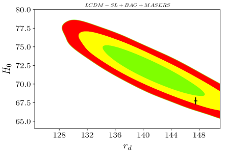
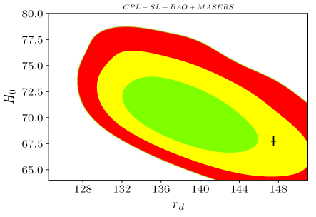
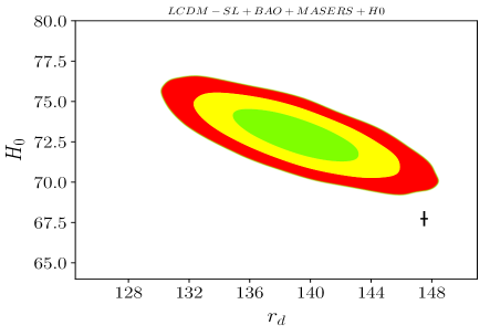
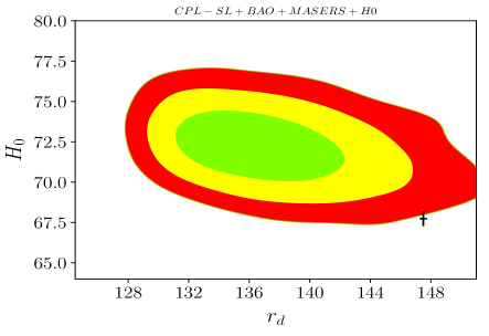
For brevity, here we provide only four examples of this comparison. In Fig. 9 one can see the two-dimensional standard error ellipses for $r_{d}$ and $H_{0}$ as calculated by the MCMC in the case of the $\Lambda$CDM models using BAO, strong lensing and megamasers with and without the distance ladder measurement of $H_{0}$. Note that, since the priors are flat in the region plotted, the marginalized likelihood and the posterior probability distribution function are proportional in this region and so the confidence regions derived from them agree.

Figure 9: An MCMC is used to calculate the standard error ellipses in $r_{d}$ and $H_{0}$ from the marginalized likelihood in the $\Lambda$CDM model (left) and CPL model (right) using BAO, lensing and masers (top) plus the distance ladder (bottom). There is excellent agreement with the corresponding panels of Figs. 4 and 6 which were calculated using the profile likelihoods.

4 Discussion

4.1 Consistency with CMB Data

So far we have seen that BAO data together with strong lensing time delays and with or without masers prefers a value of $r_{d}$ which about 2$\sigma$ below the Planck benchmark value which is determined assuming $\Lambda$CDM. Statistically significant tension arises only if one includes the local distance ladder measurement of $H_{0}$, which does little to shift the best fit value of $r_{d}$ but does reduce its uncertainty somewhat. However if future BAO and lensing measurements confirm their best fit value with increasing precision, then $r_{d}$ indeed needs to be revised downwards. There are only three ways in which this can happen.

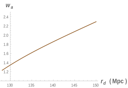
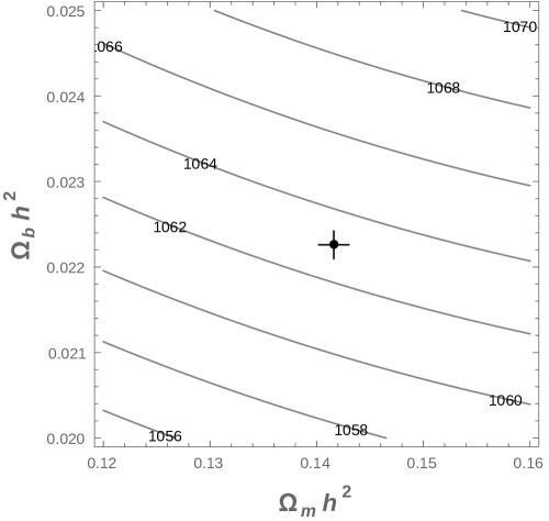
First, recall that $r_{d}$ here is measured in comoving coordinates. Thus a smaller value of $r_{d}$ does not mean that the true, metric acoustic scale is smaller. It may simply be at a higher redshift. This would require an increase in the redshift $z_{d}$ to the drag epoch of between 50 and 100. Due to the weak temperature dependence of the Saha equation together with the precisely determined CMB temperature, such a shift is actually remarkably difficult to achieve. For example, in Fig. 10 we plot the redshift of the drag epoch according to the fitting formula of Ref. [65], given a standard CDM cosmology with no dark radiation. One may observe that such a large jump in redshift would require a dramatic change in the cosmological model, likely to be quite inconsistent with mass estimates from clusters, big bang nucleosynthesis (BBN), etc. To regain consistency one would require a rather dramatic change in the model, and so we conclude that a simple reduction of $z_{d}$ is quite unlikely to resolve this tension.

Figure 10: The redshift of the drag epoch.

The second possibility is that the speed of sound of the primordial plasma needs to be reduced. This can be achieved by increasing the baryon to radiation ratio. This ratio is constrained by BBN and also by the ratios of the even to the odd acoustic peaks. One may attempt to loosen the former constraint with dark radiation or extremely early dark energy, But what about the ratios of the even to the odd peaks?

Each cosmological model gives some transfer function from the primordial perturbations to the observed CMB power spectrum. If the initial fluctuations are adiabatic, then they are characterized by a single function of the wavenumber. Given the TT power spectrum and any model, and so any transfer function, there is always some adiabatic initial condition which leads to this spectrum. Of course if one insists on a single field inflationary model then many such choices are excluded, but we are attempting to avoid such assumptions here. Therefore, if one is free to choose adiabatic initial conditions as one pleases, one can fit any TT power spectrum. Now it would require quite a fine-tuned initial spectrum to mimic the CMB acoustic peaks, since the peak locations would have to have coincidentally appeared in the initial conditions. However broader features of the power spectrum could be mimicked by broad features of the initial conditions. In the case of the damping scale it was shown in Ref. [66] that this may be achieved with the standard logarithmic running of the spectral index of the primordial fluctuations. What about even to odd peak ratios? No simple logarithmic running would do this, however it would suffice to modify just the second and fourth peaks, and so the perturbation to the primordial fluctuation power spectrum need not be so fine-tuned. We will examine this further in work in progress.

Finally, one may reduce $r_{d}$ by reducing the age of the Universe at the damping epoch. This requires either a modification of gravity or else an increase in energy, which may be early dark energy, dark radiation or something more exotic like decaying dark matter. It is the dark radiation proposal which has received the most attention in the literature. In general, it is found that dark radiation is not sufficient to remove the tension, although it certainly plays a role in scenarios such as Refs. [28, 29].

Is this reduction of $r_{d}$ consistent with CMB constraints? Perhaps one of the quantities best constrained by the CMB is the angular size of the acoustic scale $\theta_{*}$. Ignoring the small difference between the drag epoch and recombination, this is $r_{d}/D_{A}(z_{d})$. A reduction in $r_{d}$ therefore requires a proportional reduction in $D_{A}(z_{d})$. However with fixed dark energy dynamics, $D_{A}(z_{d})$ is inversely proportional to $H_{0}$. Since the BAO constraint fixes $r_{d}H_{0}$, our reduction in $r_{d}$ is already proportional to the increase in $H_{0}$ and so this angular size is automatically held fixed by the BAO constraint. This is fortunate, since a shift in the acoustic scale shifts all of the peaks in the $l$ direction, which would require a very contrived initial perturbation spectrum if one attempted to cancel its effect using initial perturbations.

On the other hand, there are other CMB constraints which are not automatically satisfied by a shift in $r_{d}$ with a compensating shift in $H_{0}$. One of these is the damping scale, which as is reviewed in Ref. [66] scales as the square root of the age of the Universe at recombination, unlike $r_{d}$ which scales linearly. This means that any mechanism which simply shifts the age at recombination, be it dark radiation or dark energy, will necessarily affect the damping scale. The observed angular size of the damping scale will increase, corresponding to less damping and so more power at high $l$. Of course this can be compensated by a running spectral index which provides less initial power at high $l$ as in Ref. [66] or by dark matter-neutrino interactions as in Ref. [67] and in the present context [68]. Such interactions are in fact always present in WIMP models of dark matter. Dark radiation will also affect the redshift of matter-radiation equality, which again affects the ratio of power at large and small $l$ and so in principle can be corrected with an appropriate shift to the running spectral index, although not a running of the same form as that which served for the damping scale.

We note however that adiabatic initial conditions only allow one function of freedom in the determination of these perturbations and so they can fit one observed power spectrum, for example TT. Polarization measurements break the degeneracy between the transfer function and the initial perturbations. Also in Ref. [25] one sees that high $l$ polarization measurements ruin the compatibility of a dark radiation model with the data. As the proliferation of parameters in fits continues, the role of polarization measurements in breaking this degeneracy will be essential.

Recently Ref. [69] has shown that the low value of $H_{0}$ obtained by Planck assuming $\Lambda$CDM can be obtained with no use of CMB data. Instead the authors used BBN data, assuming $\Lambda$CDM with no dark radiation and minimal neutrino masses, to calculate $r_{d}$. Furthermore various Dark Energy Survey measurements were included, essentially replacing the pre-recombination power spectrum measurements of the CMB with measurements of matter clustering in the recent Universe. The authors claim that such measurements are statistically independent of the Planck CMB measurement and so their consistency with the Planck value, together with moderate tension with other determinations, suggests that overall the various data sets are consistent.

One may on the other hand argue that Planck and the Ref. [69] analysis both rely heavily on the application of $\Lambda$CDM to early Universe cosmology, and that together they are statistically inconsistent with the combination of low redshift datasets provided by the local distance ladder, strong lensing time delays and the analysis presented in our study. These low redshift datasets do not make any cosmological assumptions regarding the early Universe. An inconsistency between these two sets of datasets and analyses (one with and one without assuming $\Lambda$CDM in the early Universe) therefore suggests a modification of early Universe cosmology. From this point of view the results of [69] are nonetheless important because one learns that this modification must not only preserve agreement with the power spectrum of the primordial plasma as seen in the CMB, but also the matter power spectrum at lower redshifts as observed by DES. Of course these two are closely related and so it seems plausible that one model could do both. We will investigate this problem in the sequel.

4.2 Concluding Remarks

In Ref. [60] the authors claimed that a model with modified dark energy resolves the tension between the local distance ladder $H_{0}$ and Planck. It was suggested that in the future one should investigate whether this resolution survives datasets such as BAO. We believe that the current paper answers the question posed there. BAO demands that any shift in $H_{0}$ be accompanied by a shift in $r_{d}$ and so in pre-recombination cosmology. Various combinations of strong lensing, megamasers and the local distance ladder suggest shifts of $H_{0}$ at various confidence levels, and we found that when including BAO these translate into shifts of $r_{d}$ at about the same confidence levels.

In particular, consistency between a BAO determination of $r_{d}H_{0}$ and the angular acoustic scale $r_{r}/D_{A}(z_{r})$ in the CMB implies that the angular diameter distance to recombination shifts inversely proportionally to $H_{0}$, with a small error due to the difference between the angular acoustic scale at recombination and at the drag epoch and uncertainties in late time dark energy. However the product $H_{0}D_{A}(z_{r})$ is determined entirely by the dark energy content and dynamics, and so we arrive at the following claim.

Claim: Given a shift in $H_{0}$, the consistency of BAO and the CMB angular acoustic scale measurements is maintained if and only if

$$\frac{1+z_{r}}{c}H_{0}D_{A}(z_{r})=\int_{0}^{z_{r}}\frac{dz^{\prime}}{E(z^{\prime})}=\int_{0}^{z_{r}}\frac{dz^{\prime}}{\sqrt{\Omega_{m}(1+z^{\prime})^{3}+(1-\Omega_{m})e^{3\int_{0}^{z^{\prime}}\frac{1+w(z^{\prime\prime})}{1+z^{\prime\prime}}dz^{\prime\prime}}}}$$ (4.1)

remains approximately invariant.

This does not suggest dynamical dark energy, quite on the contrary it states that at least one number calculated from the dark energy dynamics, intuitively an average acceleration, must rest invariant. It is the early time cosmology that needs to adapt to accommodate a new measurement of $H_{0}$ in the local Universe.

References

- [1] S. Perlmutter et al. [Supernova Cosmology Project Collaboration], “Discovery of a supernova explosion at half the age of the Universe and its cosmological implications,” Nature 391 (1998) 51 doi:10.1038/34124 [astro-ph/9712212].
- [2] A. G. Riess et al. [Supernova Search Team], “Observational evidence from supernovae for an accelerating universe and a cosmological constant,” Astron. J. 116 (1998) 1009 doi:10.1086/300499 [astro-ph/9805201].
- [3] S. Perlmutter et al. [Supernova Cosmology Project Collaboration], “Measurements of Omega and Lambda from 42 high redshift supernovae,” Astrophys. J. 517 (1999) 565 doi:10.1086/307221 [astro-ph/9812133].
- [4] J. Martin and R. H. Brandenberger, “The TransPlanckian problem of inflationary cosmology,” Phys. Rev. D 63 (2001) 123501 doi:10.1103/PhysRevD.63.123501 [hep-th/0005209].
- [5] M. Doran and G. Robbers, “Early dark energy cosmologies,” JCAP 0606 (2006) 026 doi:10.1088/1475-7516/2006/06/026 [astro-ph/0601544].
- [6] T. Karwal and M. Kamionkowski, “Dark energy at early times, the Hubble parameter, and the string axiverse,” Phys. Rev. D 94 (2016) no.10, 103523 doi:10.1103/PhysRevD.94.103523 [arXiv:1608.01309 [astro-ph.CO]].
- [7] V. Pettorino, L. Amendola and C. Wetterich, “How early is early dark energy?,” Phys. Rev. D 87 (2013) 083009 doi:10.1103/PhysRevD.87.083009 [arXiv:1301.5279 [astro-ph.CO]].
- [8] C. Wetterich, “The Cosmon model for an asymptotically vanishing time dependent cosmological ’constant’,” Astron. Astrophys. 301 (1995) 321 [hep-th/9408025].
- [9] M. C. Bento, O. Bertolami and A. A. Sen, “Generalized Chaplygin gas, accelerated expansion and dark energy matter unification,” Phys. Rev. D 66 (2002) 043507 doi:10.1103/PhysRevD.66.043507 [gr-qc/0202064].
- [10] L. Amendola, “Coupled quintessence,” Phys. Rev. D 62 (2000) 043511 doi:10.1103/PhysRevD.62.043511 [astro-ph/9908023].
- [11] D. Wang, Y. J. Yan and X. H. Meng, “Constraining viscous dark energy models with the latest cosmological data,” Eur. Phys. J. C 77 (2017) no.10, 660. doi:10.1140/epjc/s10052-017-5212-z
- [12] J. Evslin and S. B. Gudnason, “Dwarf Galaxy Sized Monopoles as Dark Matter?,” arXiv:1202.0560 [astro-ph.CO].
- [13] J. Markar Evslin, “Giant monopoles as a dark matter candidate,” J. Phys. Conf. Ser. 496 (2014) 012023 doi:10.1088/1742-6596/496/1/012023 [arXiv:1311.1627 [astro-ph.CO]].
- [14] S. J. Sin, “Late time cosmological phase transition and galactic halo as Bose liquid,” Phys. Rev. D 50 (1994) 3650 doi:10.1103/PhysRevD.50.3650 [hep-ph/9205208].
- [15] J. W. Lee and I. G. Koh, “Galactic halos as boson stars,” Phys. Rev. D 53 (1996) 2236 doi:10.1103/PhysRevD.53.2236 [hep-ph/9507385].
- [16] E. Di Valentino, A. Melchiorri and O. Mena, “Can interacting dark energy solve the tension?,” Phys. Rev. D 96 (2017) no.4, 043503 doi:10.1103/PhysRevD.96.043503 [arXiv:1704.08342 [astro-ph.CO]].
- [17] A. Frolop and D. Scott, “Pi in the sky,” arXiv:1603.09703 [astro-ph.CO].
- [18] G. Dvali and L. Funcke, “Small neutrino masses from gravitational θ-term,” Phys. Rev. D 93 (2016) no.11, 113002 doi:10.1103/PhysRevD.93.113002 [arXiv:1602.03191 [hep-ph]].
- [19] S. M. Koksbang and S. Hannestad, “Constraining dynamical neutrino mass generation with cosmological data,” JCAP 1709 (2017) no.09, 014 doi:10.1088/1475-7516/2017/09/014 [arXiv:1707.02579 [astro-ph.CO]].
- [20] A. Heavens, R. Jimenez and L. Verde, “Standard rulers, candles, and clocks from the low-redshift Universe,” Phys. Rev. Lett. 113 (2014) no.24, 241302 doi:10.1103/PhysRevLett.113.241302 [arXiv:1409.6217 [astro-ph.CO]].
- [21] M. Chevallier and D. Polarski, “Accelerating universes with scaling dark matter,” Int. J. Mod. Phys. D 10 (2001) 213 doi:10.1142/S0218271801000822 [gr-qc/0009008].
- [22] E. V. Linder, “Exploring the expansion history of the universe,” Phys. Rev. Lett. 90 (2003) 091301 doi:10.1103/PhysRevLett.90.091301 [astro-ph/0208512].
- [23] P. A. R. Ade et al. [Planck Collaboration], “Planck 2015 results. XIII. Cosmological parameters,” Astron. Astrophys. 594 (2016) A13 doi:10.1051/0004-6361/201525830 [arXiv:1502.01589 [astro-ph.CO]].
- [24] A. G. Riess et al., “A 2.4% Determination of the Local Value of the Hubble Constant,” Astrophys. J. 826 (2016) no.1, 56 doi:10.3847/0004-637X/826/1/56 [arXiv:1604.01424 [astro-ph.CO]].
- [25] J. L. Bernal, L. Verde and A. G. Riess, “The trouble with ,” JCAP 1610 (2016) no.10, 019 doi:10.1088/1475-7516/2016/10/019 [arXiv:1607.05617 [astro-ph.CO]].
- [26] S. Joudaki, M. Kaplinghat, R. Keeley and D. Kirkby, “Model independent inference of the expansion history and implications for the growth of structure,” arXiv:1710.04236 [astro-ph.CO].
- [27] M. Jaber and A. de la Macorra, “Probing a Steep EoS for Dark Energy with latest observations,” arXiv:1708.08529 [astro-ph.CO].
- [28] E. Di Valentino, A. Melchiorri and J. Silk, “Reconciling Planck with the local value of in extended parameter space,” Phys. Lett. B 761 (2016) 242 doi:10.1016/j.physletb.2016.08.043 [arXiv:1606.00634 [astro-ph.CO]].
- [29] E. Di Valentino, A. Melchiorri, E. V. Linder and J. Silk, “Constraining Dark Energy Dynamics in Extended Parameter Space,” Phys. Rev. D 96 (2017) no.2, 023523 doi:10.1103/PhysRevD.96.023523 [arXiv:1704.00762 [astro-ph.CO]].
- [30] D. M. Xia and S. Wang, “Constraining interacting dark energy models with latest cosmological observations,” Mon. Not. Roy. Astron. Soc. 463 (2016) no.1, 952 doi:10.1093/mnras/stw2073 [arXiv:1608.04545 [astro-ph.CO]].
- [31] J. Evslin, “Isolating the Lyman Alpha Forest BAO Anomaly,” JCAP 1704 (2017) 024 doi:10.1088/1475-7516/2017/04/024 [arXiv:1604.02809 [astro-ph.CO]].
- [32] F. Beutler et al., “The 6dF Galaxy Survey: Baryon Acoustic Oscillations and the Local Hubble Constant,” Mon. Not. Roy. Astron. Soc. 416 (2011) 3017 doi:10.1111/j.1365-2966.2011.19250.x [arXiv:1106.3366 [astro-ph.CO]].
- [33] A. J. Ross, L. Samushia, C. Howlett, W. J. Percival, A. Burden and M. Manera, “The clustering of the SDSS DR7 main Galaxy sample – I. A 4 per cent distance measure at ,” Mon. Not. Roy. Astron. Soc. 449 (2015) no.1, 835 doi:10.1093/mnras/stv154 [arXiv:1409.3242 [astro-ph.CO]].
- [34] M. Ata et al., “The clustering of the SDSS-IV extended Baryon Oscillation Spectroscopic Survey DR14 quasar sample: First measurement of Baryon Acoustic Oscillations between redshift 0.8 and 2.2,” arXiv:1705.06373 [astro-ph.CO].
- [35] S. Alam et al. [BOSS Collaboration], “The clustering of galaxies in the completed SDSS-III Baryon Oscillation Spectroscopic Survey: cosmological analysis of the DR12 galaxy sample,” Mon. Not. Roy. Astron. Soc. 470 (2017) no.3, 2617 doi:10.1093/mnras/stx721 [arXiv:1607.03155 [astro-ph.CO]].
- [36] H. du Mas des Bourboux et al., “Baryon acoustic oscillations from the complete SDSS-III Ly-quasar cross-correlation function at ,” arXiv:1708.02225 [astro-ph.CO].
- [37] M. Moresco, R. Jimenez, A. Cimatti and L. Pozzetti, “Constraining the expansion rate of the Universe using low-redshift ellipticals as cosmic chronometers,” JCAP 1103 (2011) 045 doi:10.1088/1475-7516/2011/03/045 [arXiv:1010.0831 [astro-ph.CO]].
- [38] G. B. Zhao et al., Mon. Not. Roy. Astron. Soc. 457 (2016) no.3, 2377 doi:10.1093/mnras/stw135 [arXiv:1510.08216 [astro-ph.CO]].
- [39] M. L. Wilson, A. I. Zabludoff, C. R. Keeton, K. C. Wong, K. A. Williams, K. D. French and I. G. Momcheva, “A Spectroscopic Survey of the Fields of 28 Strong Gravitational Lenses: Implications for ,” arXiv:1710.09900 [astro-ph.GA].
- [40] E. E. Falco, M. V. Gorenstein, I. I. Shapiro, “On model-dependent bounds on from gravitational images Application of Q0957 + 561A,B,” Apjl. 289 (1985) L1.
- [41] P. Schneider and D. Sluse, “Source-position transformation – an approximate invariance in strong gravitational lensing,” Astron. Astrophys. 564 (2014) A103 doi:10.1051/0004-6361/201322106 [arXiv:1306.4675 [astro-ph.CO]].
- [42] H. Dejonghe, ‘ ‘A completely analytical family of anisotropic Plummer models,” Mon. Not. Roy. Astron. Soc. 133 (1987) 217.
- [43] P. Schneider and D. Sluse, “Mass-sheet degeneracy, power-law models and external convergence: Impact on the determination of the Hubble constant from gravitational lensing,” Astron. Astrophys. 559 (2013) A37 doi:10.1051/0004-6361/201321882 [arXiv:1306.0901 [astro-ph.CO]].
- [44] J. B. Mu oz and M. Kamionkowski, “Large-Distance Lens Uncertainties and Time-Delay Measurements of ,” arXiv:1708.08454 [astro-ph.CO].
- [45] K. C. Wong et al., “H0LiCOW IV. Lens mass model of HE 0435?1223 and blind measurement of its time-delay distance for cosmology,” Mon. Not. Roy. Astron. Soc. 465 (2017) no.4, 4895 doi:10.1093/mnras/stw3077 [arXiv:1607.01403 [astro-ph.CO]].
- [46] A. J. Shajib, T. Treu and A. Agnello, “Improving time-delay cosmography with spatially resolved kinematics,” doi:10.1093/mnras/stx2302 arXiv:1709.01517 [astro-ph.CO].
- [47] W. Skidmore et al. [TMT International Science Development Teams & TMT Science Advisory Committee], “Thirty Meter Telescope Detailed Science Case: 2015,” Res. Astron. Astrophys. 15 (2015) no.12, 1945 doi:10.1088/1674-4527/15/12/001 [arXiv:1505.01195 [astro-ph.IM]].
- [48] C. E. Rasu et al., “H0LiCOW III. Quantifying the effect of mass along the line of sight to the gravitational lens HE 0435-1223 through weighted galaxy counts,” Mon. Not. Roy. Astron. Soc. 467 (2017) 4220 [arXiv:1607.01047 [astro-ph.CO]].
- [49] S. H. Suyu et al., “H0LiCOW I. Lenses in COSMOGRAIL’s Wellspring: program overview,” Mon. Not. Roy. Astron. Soc. 468 (2017) no.3, 2590 doi:10.1093/mnras/stx483 [arXiv:1607.00017 [astro-ph.CO]].
- [50] V. Bonvin et al., “H0LiCOW V. New COSMOGRAIL time delays of HE 0435?1223: to 3.8 per cent precision from strong lensing in a flat ?CDM model,” Mon. Not. Roy. Astron. Soc. 465 (2017) no.4, 4914 doi:10.1093/mnras/stw3006 [arXiv:1607.01790 [astro-ph.CO]].
- [51] S. H. Suyu, P. J. Marshall, M. W. Auger, S. Hilbert, R. D. Blandford, L. V. E. Koopmans, C. D. Fassnacht and T. Treu, “Dissecting the Gravitational Lens B1608+656. II. Precision Measurements of the Hubble Constant, Spatial Curvature, and the Dark Energy Equation of State,” Astrophys. J. 711 (2010) 201 doi:10.1088/0004-637X/711/1/201 [arXiv:0910.2773 [astro-ph.CO]].
- [52] S. H. Suyu et al., “Cosmology from gravitational lens time delays and Planck data,” Astrophys. J. 788 (2014) L35 doi:10.1088/2041-8205/788/2/L35 [arXiv:1306.4732 [astro-ph.CO]].
- [53] M. J. Reid, J. A. Braatz, J. J. Condon, L. J. Greenhill, C. Henkel and K. Y. Lo, “The Megamaser Cosmology Project: I. VLBI observations of UGC 3789,” Astrophys. J. 695 (2009) 287 doi:10.1088/0004-637X/695/1/287 [arXiv:0811.4345 [astro-ph]].
- [54] M. J. Reid, J. A. Braatz, J. J. Condon, K. Y. Lo, C. Y. Kuo, C. M. V. Impellizzeri and C. Henkel, “The Megamaser Cosmology Project: IV. A Direct Measurement of the Hubble Constant from UGC 3789,” Astrophys. J. 767 (2013) 154 doi:10.1088/0004-637X/767/2/154 [arXiv:1207.7292 [astro-ph.CO]].
- [55] C. Kuo, J. A. Braatz, M. J. Reid, F. K. Y. Lo, J. J. Condon, C. M. V. Impellizzeri and C. Henkel, “The Megamaser Cosmology Project. V. An Angular Diameter Distance to NGC 6264 at 140 Mpc,” Astrophys. J. 767 (2013) 155 doi:10.1088/0004-637X/767/2/155 [arXiv:1207.7273 [astro-ph.CO]].
- [56] F. Gao et al., “The Megamaser Cosmology Project VIII. A Geometric Distance to NGC 5765b,” Astrophys. J. 817 (2016) no.2, 128 doi:10.3847/0004-637X/817/2/128 [arXiv:1511.08311 [astro-ph.GA]].
- [57] C. Y. Kuo et al., “The Megamaser Cosmology Project. VI. Observations of NGC 6323,” Astrophys. J. 800 (2015) no.1, 26 doi:10.1088/0004-637X/800/1/26 [arXiv:1411.5106 [astro-ph.GA]].
- [58] B. P. Abbott et al. [The LIGO Scientific and The Virgo and The 1M2H and The Dark Energy Camera GW-EM and the DES and The DLT40 and The Las Cumbres Observatory and The VINROUGE and The MASTER Collaborations], “A gravitational-wave standard siren measurement of the Hubble constant,” Nature (2017) Letter Preview, doi:10.1038/nature24471 [arXiv:1710.05835 [astro-ph.CO]].
- [59] C. Guidorzi et al., “Improved constraints on H0 from a combined analysis of gravitational-wave and electromagnetic emission from GW170817,” [arXiv:1710.06426 [astro-ph.CO]].
- [60] E. Di Valentino, E. Linder and A. Melchiorri, “A Vacuum Phase Transition Solves Tension,” arXiv:1710.02153 [astro-ph.CO].
- [61] W. M. Patefield, “On the Maximized Likelihood Function,” Sankhya, Ser. B, 39 (1977) 92.
- [62] S. A. Murphy and A. W. van der Vaart, “Semiparametric likelihood ratio inference,” Ann. Statist. 25 (1997), Vol 4, 1471.
- [63] D. Foreman-Mackey, D. W. Hogg, D. Lang and J. Goodman, “emcee: The MCMC Hammer,” Publ. Astron. Soc. Pac. 125 (2013) 306 doi:10.1086/670067 [arXiv:1202.3665 [astro-ph.IM]].
- [64] Publicly available code in python ”getdist” (https://github.com/cmbant/getdist)
- [65] W. Hu and N. Sugiyama, “Small scale cosmological perturbations: An Analytic approach,” Astrophys. J. 471 (1996) 542 doi:10.1086/177989 [astro-ph/9510117].
- [66] Z. Hou, R. Keisler, L. Knox, M. Millea and C. Reichardt, “How Massless Neutrinos Affect the Cosmic Microwave Background Damping Tail,” Phys. Rev. D 87 (2013) 083008 doi:10.1103/PhysRevD.87.083008 [arXiv:1104.2333 [astro-ph.CO]].
- [67] R. J. Wilkinson, C. Boehm and J. Lesgourgues, “Constraining Dark Matter-Neutrino Interactions using the CMB and Large-Scale Structure,” JCAP 1405 (2014) 011 doi:10.1088/1475-7516/2014/05/011 [arXiv:1401.7597 [astro-ph.CO]].
- [68] E. Di Valentino, C. B. hm, E. Hivon and F. R. Bouchet, “Reducing the and tensions with Dark Matter-neutrino interactions,” arXiv:1710.02559 [astro-ph.CO].
- [69] T. M. C. Abbott et al. [DES Collaboration], “Dark Energy Survey Year 1 Results: A Precise H0 Measurement from DES Y1, BAO, and D/H Data,” arXiv:1711.00403 [astro-ph.CO].
- [70] D. Wang and X. H. Meng, “No evidence for dynamical dark energy in two models,” arXiv:1709.01074 [astro-ph.CO].
- [71] A. I. Lonappan, Ruchika and A. A. Sen, “Is it time to go beyond CDM universe?,” arXiv:1705.07336 [astro-ph.CO].