The global existence of solutions and their asymptotic stability for a reaction-diffusion system

Abstract

This paper studies the solutions of a reaction–diffusion system with nonlinearities that generalize the Lengyel–Epstein and FitzHugh–Nagumo nonlinearities. Sufficient conditions are derived for the global asymptotic stability of the system’s solutions. Furthermore, we present some numerical examples.

1 Introduction

Reaction–diffusion systems are of great importance in many scientific and engineering fields due to their ability to model numerous real life phenomena. one of the most interesting of these phenomena is that of morphogenesis, which is the biological process that causes organisms to develop specific shapes and patterns. One of the very early works on morphogenesis was conducted by Alan Turing in 1952 [16], where he anticipated that diffusion driven instability in reaction–diffusion systems leads to pattern formation. This theory was confirmed by the concrete experiment of De–Kepper et al. [6] many decades later through the chlorite–iodide–malonic acid–starch (CIMA) chemical reaction in an open unstirred gel reactor. A model referred to as Lengyel–Epstein was soon developped for the experiment in [10, 11].

Many studies have been carried out on the dynamics of the Lengyel–Epstein model. The study of Jang et al. [9] concerns the global bifurcation structure of the set of non-constant steady states in the one-dimensional case. The study in [14] looked further into the analytic characteristics of the model and showed that the initial concentrations, size of reactor, and diffusion rates must be sufficiently large to achieve Turing instability. The precise conditions on the model’s parameters that lead to the instability were later coined in [19]. The same authors also considered the global asymptotic behaviour of the model in [20]. Dynamics of the two-dimensional case where discussed in [17]. The findings of [14] and [20] in terms of the sufficient conditions for global asymptotic stability were confirmed and extended in [12].

Since the Lengyel–Epstein model only considers a single reaction, it is of particular importance to generalise its reactions terms to encompass other variations of the model. A first attempt to generalise the model was achieved in [1], where it was shown how other approximations of the reaction term could be studied in a general way. The same model was studied again in [2], where the authors estabished sufficient conditions for the non–existence of Turing patterns. The authors also followed on the footsteps of [12] to relax the global asymptotic stability conditions. Another study related to the same model is [3], whre the authors established the boundedness of solutions.

This paper presents a broader generalisation of the Lengyel–Epstein model to encompass many existing systems such as the FitzHugh–Nagumo model [15, 7] as will be shown later on in Section 7. In Section 2, we will present the general model proposed in this paper. In the consequent sections, we will study the dynamics of the proposed system.

2 System Model

In this paper, we consider the reaction–diffusion system

$$\left\{\begin{array}[]{l}\frac{\partial u}{\partial t}-d_{1}\Delta u=\left(f\left(u\right)-\lambda v\right)\varphi\left(u\right):=F\left(u,v\right)\text{ \ \ \ in }\mathbb{R}^{+}\times\Omega,\vskip 3.0pt plus 1.0pt minus 1.0pt\\ \frac{\partial v}{\partial t}-d_{2}\Delta v=\sigma\left(g\left(u\right)-v\right)\varphi\left(u\right):=G\left(u,v\right)\text{ \ \ \ in }\mathbb{R}^{+}\times\Omega,\end{array}\right.$$ (2.1)

where $\Omega$ is a bounded domain in $\mathbb{R}^{n}$ with smooth boundary $\partial\Omega$ and $\Delta$ is the Laplacian operator on $\Omega$. We assume non-negative continuous and bounded initial data

$$u\left(0,x\right)=u_{0}\left(x\right),\text{ \ }v\left(0,x\right)=v_{0}\left(x\right)\text{ \ \ \ \ \ \ \ \ \ \ in }\Omega,$$ (2.2)

where $u_{0}\left(x\right),v_{0}\left(x\right)\in C^{2}\left(\Omega\right)\cap C\left(\overline{\Omega}\right)$, and homogoneous Neumann boundary conditions

$$\dfrac{\partial u}{\partial\nu}=\dfrac{\partial v}{\partial\nu}=0\ \ \text{\ \ \ \ \ on \ \ \ }\mathbb{R}^{+}\times\partial\Omega,$$ (2.3)

with $\nu$ being the unit outer normal to $\partial\Omega$.

The constants $d_{1},d_{2},\lambda,$ and $\sigma$ are assumed to be strictly positive control parameters. Note that $d_{1}$ and $d_{2}$ represent the diffusivity constants, which in a chemical reaction are proportional to the ratios between the molar flux and the concentration gradient of the reactants. The functions $\varphi,g$ and $f$ are assumed to be continuously differentiable on $\mathbb{R}^{+}$ such that for some $\delta\in\mathbb{R}^{+}$,

$$\varphi\left(0\right)=0,f\left(\delta\right)=0,$$ (2.4)

and for $u\in\left(0,\delta\right)$,

$$g(u),f\left(u\right),\varphi\left(u\right)>0,$$ (2.5)

and

$$g^{\prime}(u)\geq 0.$$ (2.6)

We also suppose that there exists a positive constant $\alpha\in\left(0,\delta\right)$ such that

$$\lambda g\left(\alpha\right)=f\left(\alpha\right),$$ (2.7)

and

$$\left(\alpha-u\right)\left[f\left(u\right)-\lambda g\left(u\right)\right]>0\text{ \ for\ }u\in\left(0,\alpha\right)\cup\left(\alpha,\delta\right).$$ (2.8)

3 Preliminaries

In this section, we will present some preliminary results. First, we show that subject to (2.6), the system has an invariant region. Then, we identify a unique equilibrium solution for the ODE system and establish its local asymptotic stability under certain conditions. Finally, the local asymptotic stability of the steady state solution in the presence of diffusions is established under some sufficient conditions.

3.1 Invariant Regions

In this subsection, we examine the invariant regions for the system (2.1).

Definition 1 ([20, 13])

A rectangle $\Re=\left(0,r_{1}\right)\times\left(0,r_{2}\right)$ is called an invariant rectangle if the vector field $\left(F,G\right)$ on the boundary $\partial\Re$ points inside, that is,

$$\left\{\begin{array}[]{c}F\left(0,v\right)\geq 0\text{ and }F\left(r_{1},v\right)\leq 0\text{ for }0<v<r_{2},\\ G\left(u,0\right)\geq 0\text{ and }G\left(u,r_{2}\right)\leq 0\text{ for }0<u<r_{1}.\end{array}\right.$$

Proposition 1

The system (2.1), with condition (2.6) has the invariant region

$$\Re=\left(0,\delta\right)\times\left(0,g\left(\delta\right)\right).$$

Proof:

From condition (2.4), we obtain

$$F\left(0,v\right)=\lim_{u\rightarrow 0^{+}}f\left(u\right)\varphi\left(u\right)\geq 0.$$

Also, using (2.4) and (2.7), we conclude that

$$\left(f\left(\delta\right)-f\left(\alpha\right)\right)-\lambda v-g\left(\alpha\right)=-\left(1+\lambda\right)g\left(\alpha\right)-\lambda v\leq 0.$$

It follows that

$$F\left(\delta,v\right)=\left[\left(f\left(\delta\right)-f\left(\alpha\right)\right)-\lambda\left(v-g\left(\alpha\right)\right)\right]\varphi\left(\delta\right)\leq 0,$$

$$G\left(u,0\right)=\sigma\varphi\left(u\right)\left(g\left(u\right)-0\right)=\sigma\varphi\left(u\right)g\left(u\right)\geq 0,$$

and

$$G\left(u,g\left(\delta\right)\right)=\sigma\varphi\left(u\right)\left(g\left(u\right)-g\left(\delta\right)\right)\leq 0.$$

This concludes the proof. $\square$

3.2 Equilibrium Solutions and ODE Stability

This section studies the uniform equilibrium solutions of the reaction–diffusion system (2.1). In the absense of diffusion, the system reduces to

$$\left\{\begin{array}[]{l}\frac{du}{dt}=\varphi\left(u\right)\left(f\left(u\right)-\lambda v\right)\text{ \ \ in }\mathbb{R}^{+},\vskip 3.0pt plus 1.0pt minus 1.0pt\\ \frac{dv}{dt}=\frac{\sigma}{\lambda}\varphi\left(u\right)\left(\lambda g\left(u\right)-\lambda v\right)\text{ \ \ in }\mathbb{R}^{+}.\end{array}\right.$$ (3.1)

Proposition 2

The system (3.1) has the unique constant steady state solution

$$\left(u^{\ast},v^{\ast}\right)=\left(\alpha,g\left(\alpha\right)\right).$$ (3.2)

If the inequality

$$f^{\prime}\left(\alpha\right)<\min\left\{\sigma,\lambda g^{\prime}\left(\alpha\right)\right\}$$ (3.3)

is satisfied, then the solution is a locally asymptotically stable equilibrium for the system (3.1).

Proof:

An equilibrium solution $\left(u^{\ast},v^{\ast}\right)$ satisfies

$$\left\{\begin{array}[]{l}\left[\left(f\left(u^{\ast}\right)-f\left(\alpha\right)\right)-\lambda\left(v^{\ast}-g\left(\alpha\right)\right)\right]\varphi\left(u^{\ast}\right)=0,\\ \sigma\left[\left(g\left(u^{\ast}\right)-g\left(\alpha\right)\right)-\left(v^{\ast}-g\left(\alpha\right)\right)\right]\varphi\left(u^{\ast}\right)=0.\end{array}\right.$$

It is easy to see that $\left(\alpha,g\left(\alpha\right)\right)$ is the solution to this system thanks to conditions (2.7) and (2.8). It remains now to study the local asymptotic stability of the solution. The Jacobian matrix is

$$J\left(u,v\right)=\left(\begin{array}[]{cc}F_{u}\left(u,v\right)&F_{v}\left(u,v\right)\\ G_{u}\left(u,v\right)&G_{v}\left(u,v\right)\end{array}\right),$$ (3.4)

where

$$F_{v}=-\lambda\varphi\left(u\right),\ \ G_{v}=-\sigma\varphi\left(u\right),$$

$$F_{u}=\left(\left[\left(f\left(u\right)-f\left(\alpha\right)\right)-\lambda\left(v-g\left(\alpha\right)\right)\right]\varphi^{\prime}\left(u\right)+f^{\prime}\left(u\right)\varphi\left(u\right)\right),$$

and

$$G_{u}=\sigma\left(\left(g\left(u\right)-v\right)\varphi^{\prime}\left(u\right)+g^{\prime}\left(u\right)\varphi\left(u\right)\right).$$

Evaluating these derivatives for the equilibrium solution yields

$$F_{v}\left(\alpha,g\left(\alpha\right)\right)=-\lambda\varphi\left(\alpha\right),$$

$$G_{v}\left(\alpha,g\left(\alpha\right)\right)=-\sigma\varphi\left(\alpha\right),$$

$$F_{u}\left(\alpha,g\left(\alpha\right)\right) = \left(\left[\left(f\left(\alpha\right)-f\left(\alpha\right)\right)-\lambda\left(g\left(\alpha\right)-g\left(\alpha\right)\right)\right]\varphi^{\prime}\left(\alpha\right)+f^{\prime}\left(\alpha\right)\varphi\left(\alpha\right)\right)$$

$$= f^{\prime}\left(\alpha\right)\varphi\left(\alpha\right),$$

and

$$G_{u}\left(\alpha,g\left(\alpha\right)\right)=\sigma g^{\prime}\left(\alpha\right)\varphi\left(\alpha\right).$$

Consequently,

$$J\left(u^{\ast},v^{\ast}\right)=\left(\begin{array}[]{cc}f^{\prime}\left(\alpha\right)\varphi\left(\alpha\right)&-\lambda\varphi\left(\alpha\right)\\ \sigma g^{\prime}\left(\alpha\right)\varphi\left(\alpha\right)&-\sigma\varphi\left(\alpha\right)\end{array}\right).$$

As the trace given by

$${\text{tr}}J\left(u^{\ast},v^{\ast}\right)=\left[f^{\prime}\left(\alpha\right)-\sigma\right]\varphi\left(\alpha\right)<0,$$

and the determinant given by

$$\det J\left(u^{\ast},v^{\ast}\right)=\sigma\varphi^{2}\left(\alpha\right)\left[\lambda g^{\prime}\left(\alpha\right)-f^{\prime}\left(\alpha\right)\right]>0,$$ (3.5)

the equilibrium is then locally asymptotically stable. $\square$

Remark 1

Observe that $F_{v}\left(u^{\ast},v^{\ast}\right)<0,$ $G_{v}\left(u^{\ast},v^{\ast}\right)<0$ and $G_{u}\left(u^{\ast},v^{\ast}\right)>0$. Recall that $\varphi\left(\alpha\right)$ is strictly positive. Hence, if

$$F_{u}\left(u^{\ast},v^{\ast}\right)=f^{\prime}\left(\alpha\right)\varphi\left(\alpha\right)>0$$ (3.6)

is satisfied, then $u$ is called an activator, $v$ is called an inhibitor, and the system (3.1) is an activator–inhibitor system.

Remark 2

Combining the activator-inhibitor condition (3.6) with the stability condition (3.3), we find that the condition

$$0<f^{\prime}\left(\alpha\right)<\min\left\{\sigma,\lambda g^{\prime}\left(\alpha\right)\right\}$$ (3.7)

makes the model (3.1) a diffusion-free stable activator-inhibitor system.

3.3 PDE Stability

Let us consider the local asymptotic stability of the steady state solutions in the PDE case. Let $0=\lambda_{0}<\lambda_{1}\leq\lambda_{3}\leq....$ be the sequence of eigenvalues for ($-\Delta$) subject to the Neumann boundary conditions on $\Omega,$ where each $\lambda_{i}$ has multiplicity $m_{i}\geq 1$. Also let $\Phi_{ij},1\leq j\leq m_{i}$, (recall that $\Phi_{0}=const$ and $\lambda_{i}\rightarrow\infty$ at $i\rightarrow\infty$) be the normalized eigenfunctions corresponding to $\lambda_{i}$. That is, $\Phi_{ij}$ and $\lambda_{i}$ satisfy $-\Delta\Phi_{ij}=\lambda_{i}\Phi_{ij}$ in $\Omega$, with $\frac{\partial\Phi_{ij}}{\partial\nu}=0$ in $\partial\Omega$, and $\int_{\Omega}\Phi_{ij}^{2}\left(x\right)dx=1$.

The set $\left\{\Phi_{ij}:i\geq 0,1\leq j\leq m_{i}\right\}$ forms a complete orthonormal basis in $L^{2}\left(\Omega\right)$. If

$$d_{1}\lambda_{1}<F_{0}:=f^{\prime}\left(\alpha\right)\varphi\left(\alpha\right),$$ (3.8)

then we may define $i_{\alpha}=i_{\alpha}(\alpha,\Omega)$ to be the largest positive integer such that

$$d_{1}\lambda_{i}<F_{0}\text{ \ \ for all\ \ }i\leq i_{\alpha}.$$

Clearly, if (3.8) is satisfied, then $1\leq i_{\alpha}<\infty$. In this case, we define

$$d=d\left(\alpha,\Omega\right)=\underset{1\leq i<i_{\alpha}}{\min}\widetilde{d}_{i},\text{ \ }\widetilde{d}_{i}=\varphi\left(\alpha\right)\frac{\lambda_{i}d_{1}+\varphi\left(\alpha\right)\left(\lambda g^{\prime}\left(\alpha\right)-f^{\prime}\left(\alpha\right)\right)}{\lambda_{i}\left(F_{0}-\lambda_{i}d_{1}\right)}.$$ (3.9)

Proposition 3

Subject to (3.7), if either $\lambda_{1}d_{1}\geq F_{0}$ or $\lambda_{1}d_{1}<F_{0}$ and $0<\frac{d_{2}}{\sigma}<d$, then the constant steady state $\left(u^{\ast},v^{\ast}\right)$ is locally asymptotically stable. Otherwise, if  $\lambda_{1}d_{1}<F_{0}$ and $d<\frac{d_{2}}{\sigma}$, then $\left(u^{\ast},v^{\ast}\right)$ is locally asymptotically unstable.

Proof:

First, let us define the operator

$$L =\left(\begin{array}[]{cc}d_{1}\Delta+f^{\prime}\left(\alpha\right)\varphi\left(\alpha\right)&-\lambda\varphi\left(\alpha\right)\\ \sigma g^{\prime}\left(\alpha\right)\varphi\left(\alpha\right)&d_{2}\Delta-\sigma\varphi\left(\alpha\right)\end{array}\right)$$

$$=\left(\begin{array}[]{cc}d_{1}\Delta+F_{0}&F_{1}\\ \sigma G_{0}&d_{2}\Delta+\sigma G_{1}\end{array}\right).$$

The steady state solution $\left(u^{\ast},v^{\ast}\right)$ is locally assymptotically stable if all the eigenvalues of $L$ have negative real parts, see for instance [5]. On the contrary, if some eigenvalues have positive real parts, then the steady state is locally asymptotically unstable. We have

$$L\left(\phi\left(x\right),\psi\left(x\right)\right)^{t}=\xi\left(\phi\left(x\right),\psi\left(x\right)\right)^{t},$$

where $\left(\phi\left(x\right),\psi\left(x\right)\right)$ is an eigenfunction of $L$ corresponding to an eigenvalue $\xi$; this can be rearranged to

$$\left(\begin{array}[]{cc}d_{1}\Delta+F_{0}-\xi&F_{1}\\ \sigma G_{0}&d_{2}\Delta+\sigma G_{1}-\xi\end{array}\right)\left(\begin{array}[]{c}\phi\\ \psi\end{array}\right)=\left(\begin{array}[]{c}0\\ 0\end{array}\right),$$

which can be rewritten as

$$\sum_{0\leq i\leq\infty,1\leq j\leq m_{i}}\left(\begin{array}[]{cc}F_{0}-d_{1}\lambda_{i}-\xi&F_{1}\\ \sigma G_{0}&\sigma G_{1}-d_{2}\lambda_{i}-\xi\end{array}\right)\left(\begin{array}[]{c}a_{ij}\\ b_{ij}\end{array}\right)\Phi_{ij}=\left(\begin{array}[]{c}0\\ 0\end{array}\right),$$

where

$$\phi=\sum_{0\leq i\leq\infty,1\leq j\leq m_{i}}a_{ij}\Phi_{ij},$$

and

$$\psi=\sum_{0\leq i\leq\infty,1\leq j\leq m_{i}}b_{ij}\Phi_{ij}.$$

Observe that

$$\det\left(\begin{array}[]{cc}F_{0}-d_{1}\lambda_{i}-\xi&F_{1}\\ \sigma G_{0}&\sigma G_{1}-d_{2}\lambda_{i}-\xi\end{array}\right)=\xi^{2}+p_{i}\xi+Q_{i},$$

with

$$p_{i} =\left(\lambda_{i}d_{1}-\sigma G_{1}-F_{0}+\lambda_{i}d_{2}\right)$$

$$=\left(d_{1}+d_{2}\right)\lambda_{i}+\left[\sigma-f^{\prime}\left(\alpha\right)\right]\varphi\left(\alpha\right)>0,$$

by condition (3.7), and

$$Q_{i} =\lambda_{i}^{2}d_{1}d_{2}+\sigma F_{0}G_{1}-\lambda_{i}F_{0}d_{2}-\sigma\lambda_{i}G_{1}d_{1}-\sigma F_{1}G_{0}$$

$$=\sigma\left[\lambda_{i}\frac{d_{2}}{\sigma}\left(\lambda_{i}d_{1}-F_{0}\right)-G_{1}\lambda_{i}d_{1}+F_{0}G_{1}-F_{1}G_{0}\right]$$

$$=\sigma\left[\frac{d_{2}}{\sigma}\lambda_{i}\left(\lambda_{i}d_{1}-F_{0}\right)+\varphi\left(\alpha\right)\left\{\lambda_{i}d_{1}+\varphi\left(\alpha\right)\left(\lambda g^{\prime}\left(\alpha\right)-f^{\prime}\left(\alpha\right)\right)\right\}\right];$$

note that $Q_{0}>0$ for $\lambda_{0}=0$. Hence, one may easily observe that $\xi$ is an eigenvalue of $L$ iff for some $i\geq 0$,

$$\xi^{2}+p_{i}\xi+Q_{i}=0.$$

We can study the three cases stated in the proposition above separately:

1. If $\lambda_{1}d_{1}\geq F_{0}$, then $Q_{i}>0$ for $i\geq 1$. The fact that for $i\geq 0$, both $p_{i}>0$ and $Q_{i}>0$ for $i\geq 0$ implies that $\text{Re}\xi<0$ for all eigenvalues $\xi$; consequently the steady state $\left(u^{\ast},v^{\ast}\right)$ is locally asymptotically stable.

2. We consider the case where $\lambda_{1}d_{1}<F_{0}$ and $0<\frac{d_{2}}{\sigma}<d$, which leads to

   $$\lambda_{1}d_{1}<F_{0}\text{ and }0<\frac{d_{2}}{\sigma}<\widetilde{d}_{i},$$

   for $i\in\left[1,i_{\alpha}\right]$. It simply follows that $Q_{i}>0$ for $i\in\left[1,i_{\alpha}\right]$. Furthermore, if $i\geq i_{\alpha}$, then $\lambda_{i}d_{1}\geq F_{0}$ and $Q_{i}>0$; this leads to the local asymptotic stability of $\left(u^{\ast},v^{\ast}\right)$ again.

3. If $\lambda_{1}d_{1}<F_{0}$ and $d<\frac{d_{2}}{\sigma}$, then we may assume that the minimum in (3.9) is reached by $k\in\left[1,i_{\alpha}\right]$. Thus,

   $$\frac{d_{2}}{\sigma}>\widetilde{d}_{k},$$ (3.10)

   which implies $Q_{k}<0$, and consequently the instability of $\left(u^{\ast},v^{\ast}\right)$ follows.

$\square$

4 Boundedness of Solutions

In this section, we would like to establish the global existence of solutions for the system (2.1). We start by proving that it has a unique solution $\left(u\left(x,t\right),v\left(x,t\right)\right)$ for all $x\in\Omega$ and $t>0$, which is bounded by some positive constants depending on $u_{0}$ and $v_{0}$. In order to establish the boundedness of solutions, it is assumed that $\varphi\$is a sublinear function, i.e. the mapping $(0,\infty)\ni s\rightarrow\frac{\varphi(s)}{s}$ is non–increasing. In a similar manner to Lemma 1 of [1], we may establish that the sublinearity of $\varphi$ along with the first part of (2.4), $\varphi\left(0\right)=0$, gives

$$0<\frac{\varphi\left(u\right)}{u}\leq\varphi^{\prime}\left(0\right).$$ (4.1)

Let us also assume that

$$f\left(u\right)\varphi\left(u\right)=K-u\Psi\left(u\right),$$

with $K$ being a positive real number and $\Psi\left(u\right)$ a positive bounded function. Similarly, we assume that

$$g\left(u\right)\varphi\left(u\right)=u\Phi\left(u\right),$$

where $\Phi\left(u\right)$ is a positive bounded function. The following propositions are based on the work of Ni and Tang (2005) [14] for the original Lengyel–Epstein system.

Proposition 4

The system (2.1) admits a unique solution $(u,v)$ for all $x\in\Omega$ and $t>0$ and there exist two positive constants $C_{1}$ and $C_{2}$ such that

$$C_{1}<u\left(x,t\right),v\left(x,t\right)<C_{2}.$$ (4.2)

Proof:

Since the local existence and uniqueness of solutions are classical for the proposed system, see [8], it suffices to establish the global existence by proving the boundedness of the solution. To this aim, we will use the invariant regions theory as proposed in [18]. We take a certain rectangular region of the form

$$R=\left(u_{1},u_{2}\right)\times\left(v_{1},v_{2}\right),$$

and study the behavior of the vector field along its four boundaries separately.

• On the left boundary of $R$, we have $u=u_{1}$ and $v_{1}\leq v\leq v_{2}$. Hence,

  $$F\left(u,v\right) = \left(f\left(u\right)-\lambda v\right)\varphi\left(u\right)$$

  $$\geq f\left(u_{1}\right)\varphi\left(u_{1}\right)-\lambda v_{2}\varphi\left(u_{1}\right)$$

  $$\geq K-u_{1}\Psi\left(u_{1}\right)-\lambda v_{2}\varphi\left(u_{1}\right)$$

  $$\geq K-u_{1}\left[\Psi\left(u_{1}\right)+\lambda v_{2}\frac{\varphi\left(u_{1}\right)}{u_{1}}\right]$$

  $$\geq K-u_{1}\left[\Psi\left(u_{1}\right)+\lambda v_{2}\varphi^{\prime}\left(0\right)v_{2}\right].$$

  A sufficient condition for $F\left(u,v\right)\geq 0$ can then be formulated as

  $$K-u_{1}\left[\Psi\left(u_{1}\right)+\lambda v_{2}\varphi^{\prime}\left(0\right)v_{2}\right]\geq 0.$$

  Whereupon

  $$u_{1}\leq\frac{K}{\Psi_{\min}+\lambda v_{2}\varphi^{\prime}\left(0\right)}.$$

• For the right boundary where $u=u_{2}$ and $v_{1}\leq v\leq v_{2}$, we have

  $$F\left(u,v\right) = f\left(u\right)\varphi\left(u\right)-\lambda v\varphi\left(u\right)$$

  $$\leq f\left(u_{2}\right)\varphi\left(u_{2}\right)$$

  $$\leq K-u_{2}\Psi\left(u_{2}\right).$$

  It suffices that

  $$K-u_{2}\Psi\left(u_{2}\right)\leq 0,$$

  or simply

  $$\frac{K}{\Psi_{\max}}\leq u_{2},$$

  to guarantee the inquality $F\left(u,v\right)\leq 0$.

These two conditions yield the first part of the invariant region $R$:

$$u_{1}=\min\left\{\frac{K}{\Psi_{\min}+\lambda v_{2}\varphi^{\prime}\left(0\right)},\min u_{0}\right\},$$ (4.3)

and

$$u_{2}=\max\left\{\frac{K}{\Psi_{\max}},\max u_{0}\right\}.$$ (4.4)

• For the third boundary of $R$ where $v=v_{1}$ and $u_{1}\leq u\leq u_{2}$,

  $$G\left(u,v\right) = \sigma\left(g\left(u\right)\varphi\left(u\right)-v_{1}\varphi\left(u\right)\right)$$

  $$= \sigma\left(u\Phi\left(u\right)-v_{1}\varphi\left(u\right)\right)$$

  $$\geq \sigma u\left(\Phi\left(u\right)-v_{1}\frac{\varphi\left(u\right)}{u}\right)$$

  $$\geq \sigma u\left(\Phi_{\min}-v_{1}\varphi^{\prime}\left(0\right)\right).$$

  Hence, to achieve $G\left(u,v\right)\geq 0$, it suffices that

  $$v_{1}\leq\frac{\Phi_{\min}}{\varphi^{\prime}\left(0\right)}.$$

• For the boundary with $v=v_{2}$ and $u_{1}\leq u\leq u_{2}$,

  $$G\left(u,v\right) = \sigma\left(g\left(u\right)\varphi\left(u\right)-v_{2}\varphi\left(u\right)\right)$$

  $$= \sigma\left(u\Phi\left(u\right)-v_{2}\varphi\left(u\right)\right)$$

  $$= \sigma u\left(\Phi\left(u\right)-v_{2}\frac{\varphi\left(u\right)}{u}\right)$$

  $$\leq \sigma u\left(\Phi_{\max}-v_{2}\frac{\varphi\left(u_{2}\right)}{u_{2}}\right).$$

  To ensure the negativity of $G\left(u,v\right)$ on this boundary, it is sufficient to choose $v_{2}$ such that

  $$v_{2}\geq\frac{u_{2}}{\varphi\left(u_{2}\right)}\Phi_{\max}.$$

Combining the conditions for these two boundaries gives us

$$v_{1}=\min\left\{\frac{\Phi_{\min}}{\varphi^{\prime}\left(0\right)},\min v_{0}\right\},$$ (4.5)

and

$$v_{2}=\max\left\{\frac{u_{2}}{\varphi\left(u_{2}\right)}\Phi_{\max},\max v_{0}\right\}.$$ (4.6)

We can now simply define the bounds of the solutions as

$$C_{1}=\min\left\{u_{1},v_{1}\right\}>0,$$ (4.7)

and

$$C_{2}=\min\left\{u_{2},v_{2}\right\}>0.$$ (4.8)

$\square$

5 Global Asymptotic Stability

We now pass to the global asymptotic stability for the system (2.1). For the global asymptotic stability of the steady state solution, we consider the condition

$$\left(\alpha-u\right)\left[f\left(u\right)-f\left(\alpha\right)\right]>0\text{ \ for }u\in\left(0,\alpha\right)\cup\left(\alpha,\delta\right),$$ (5.1)

which is clearly stronger than (2.8). System (2.1) can now be rewritten as

$$\left\{\begin{array}[]{l}\frac{\partial u}{\partial t}-d_{1}\Delta u=\left[\left(f\left(u\right)-f\left(\alpha\right)\right)-\lambda\left(v-g\left(\alpha\right)\right)\right]\varphi\left(u\right)\text{ \ \ \ in }\mathbb{R}^{+}\times\Omega,\vskip 3.0pt plus 1.0pt minus 1.0pt\\ \frac{\partial v}{\partial t}-d_{2}\Delta v=\sigma\left[\left(g\left(u\right)-g\left(\alpha\right)\right)-\left(v-g\left(\alpha\right)\right)\right]\varphi\left(u\right)\text{ \ \ \ in }\mathbb{R}^{+}\times\Omega.\end{array}\right.$$

As a first step, we start by establishing the conditions for the global stabiliy of $\left(u^{\ast},v^{\ast}\right)$ as a solution of the reduced ODE system

$$\left\{\begin{array}[]{l}\frac{\partial u}{\partial t}=F\left(u,v\right),\vskip 3.0pt plus 1.0pt minus 1.0pt\\ \frac{\partial v}{\partial t}=G\left(u,v\right).\end{array}\right.$$ (5.2)

Theorem 1

If for all $u$ $\in\left(0,\delta\right)$,

$$f^{\prime}\left(u\right)<\sigma,$$ (5.3)

then $\left(u^{\ast},v^{\ast}\right)$ is globally asymptotically stable.

Proof:

System (5.2) may be written as

$$\left\{\begin{array}[]{l}u_{t}=\varphi\left(u\right)\left[f\left(u\right)-\lambda v\right],\\ v_{t}=\sigma\varphi\left(u\right)\left(g\left(u\right)-v\right).\end{array}\right.$$

Let us consider the vector field

$$\Psi\left(u,v\right)=\left(f\left(u\right)-\lambda v,\sigma g\left(u\right)-\sigma v\right),$$

along with its divergence

$${\text{div}}\Psi\left(u,v\right) =\frac{\partial}{\partial u}\left(f\left(u\right)-\lambda v\right)+\frac{\partial}{\partial v}\left(\sigma g\left(u\right)-\sigma v\right)$$

$$=f^{\prime}\left(u\right)-\sigma.$$

Let us also consider the open rectangle $\Re$ with closure $\overline{\Re}$. We aim to show that

$$\min_{\left(u,v\right)\in\overline{\Re}}\left({\text{div}}\Psi\left(u,v\right)\right)<0.$$ (5.4)

By combining (5.3) and (5.4), it becomes clear that

$${\text{div}}\Psi\left(u,v\right)<0\text{ in }\Re.$$

Therefore, making use of the classical Bendixson–Dulac criterion [4], system (5.2) does not admit any periodic solutions in $\Re$. It follows from the Poincaré–Bendixson theorem [4] that for any solution $\left(u\left(t\right),v\left(t\right)\right)$ to (5.2), the equality

$$\lim_{t\rightarrow\infty}\left|u\left(t\right)-u^{\ast}\right|=0=\lim_{t\rightarrow\infty}\left|v\left(t\right)-v^{\ast}\right|$$

holds. This concludes the proof. $\square$

Theorem 2

If condition (5.1) is satisfied, then for any solution $\left(u,v\right)$ to (2.1), we get

$$\lim_{t\rightarrow\infty}\left\|u\left(.,t\right)-u^{\ast}\right\|_{L^{2}\left(\Omega\right)}=\lim_{t\rightarrow\infty}\left\|v\left(.,t\right)-v^{\ast}\right\|_{L^{2}\left(\Omega\right)}=0.$$ (5.5)

Lemma 1

If $u\in\left(0,\delta\right)$, then there exists a constant $\gamma$ between $u$ and $\alpha$ such that

$$g\left(u\right)-g\left(\alpha\right)=\left(u-\alpha\right)g^{\prime}\left(\gamma\right).$$

Lemma 2

Consider the function $H$ defined as

$$H\left(u\right)=\int_{\alpha}^{u}\left(g\left(r\right)-g\left(\alpha\right)\right)dr$$ (5.6)

It follows that

$$H\left(u\right)\geq 0,\text{ \ and }\frac{d}{du}H\left(u\right)=g\left(u\right)-g\left(\alpha\right).$$

Proof:

As a result of using (1), there exists a $\gamma\left(r\right)$ in the interval $\left(\min\left\{r,\alpha\right\},\max\left\{r,\alpha\right\}\right)$ with $r$ lying between $u$ and $\alpha$ such that

$$H\left(u\left(x,t\right)\right)=\int_{\alpha}^{u}\left(r-\alpha\right)g^{\prime}\left(\gamma\right)dr,$$

where $\psi\left(\gamma\right)\geq 0$, leading to

$$\inf_{r\in\left(\min\left\{u,\alpha\right\},\max\left\{u,\alpha\right\}\right)}g^{\prime}\left(\gamma\right)\int_{\alpha}^{u}\left(r-\alpha\right)dr\leq H\left(u\left(x,t\right)\right).$$

Whereupon

$$0\leq\inf_{r}g^{\prime}\left(\gamma\right)\frac{1}{2}\left(u-\alpha\right)^{2}\leq H\left(u\left(x,t\right)\right),$$

which shows that $H\left(u\right)\geq 0$. $\square$

Proposition 5

Let $\left(u\left(t,.\right),v\left(t,.\right)\right)$ be a solution of (2.1)-(2.3) and let

$$V\left(t\right)=\int_{\Omega}E\left(u\left(x,t\right),v\left(x,t\right)\right)dx,$$ (5.7)

where

$$E\left(u,v\right)=\sigma H\left(u\right)+\frac{\lambda}{2}\left(v-v^{\ast}\right)^{2},$$ (5.8)

then subject to (5.1), $V\left(t\right)$ is a Lyapunov functional.

Proof:

First of all,

$$V\left(t\right)=\int_{\Omega}\left[\sigma H\left(u\right)+\frac{\lambda}{2}\left(v-v^{\ast}\right)^{2}\right]dx.$$

We have

$$\frac{d}{dt}V\left(t\right) =\frac{d}{dt}\int_{\Omega}\left[\sigma H\left(u\right)+\frac{\lambda}{2}\left(v-v^{\ast}\right)^{2}\right]dx$$

$$=\int_{\Omega}\sigma\frac{d}{dt}\left[H\left(u\right)\right]dx+\frac{\lambda}{2}\frac{d}{dt}\int_{\Omega}\left(v-v^{\ast}\right)^{2}dx$$

$$=\sigma\int_{\Omega}\left(g\left(u\right)-g\left(u^{\ast}\right)\right)u_{t}dx+\lambda\int_{\Omega}\left(v-v^{\ast}\right)v_{t}dx$$

$$=\sigma\int_{\Omega}\left(g\left(u\right)-g\left(u^{\ast}\right)\right)\left(d_{1}\Delta u+\varphi\left(u\right)\left[\left(f\left(u\right)-f\left(u^{\ast}\right)\right)-\lambda\left(v-v^{\ast}\right)\right]\right)dx$$

$$\ \ \ \ \ \ \ \ +\lambda\int_{\Omega}\left(v-v^{\ast}\right)\left(d_{2}\Delta u+\sigma\varphi\left(u\right)\left[\left(g\left(u\right)-g\left(u^{\ast}\right)\right)-\left(v-v^{\ast}\right)\right]\right)dx.$$

For reasons that will become clear at the end of this proof, let us set

$$I=\sigma d_{1}\int_{\Omega}\left(g\left(u\right)-g\left(u^{\ast}\right)\right)\Delta u\,dx+\lambda d_{2}\int_{\Omega}\left(v-v^{\ast}\right)\Delta v\,dx,$$

and

$$J=\int_{\Omega}\sigma\varphi\left(u\right)\left[\left(g\left(u\right)-g\left(u^{\ast}\right)\right)\left(f\left(u\right)-f\left(u^{\ast}\right)\right)-\lambda\left(v-v^{\ast}\right)^{2}\right]dx.$$

Let us also set

$$I=I_{1}+I_{2},$$

where

$$I_{1} =\sigma d_{1}\int_{\Omega}\left(g\left(u\right)-g\left(u^{\ast}\right)\right)\Delta u\,dx$$

$$=-\sigma d_{1}\int_{\Omega}g^{\prime}\left(u\right)\left|\nabla u\right|^{2}\,dx,$$

and

$$I_{2} =\lambda d_{2}\int_{\Omega}\left(v-v^{\ast}\right)\Delta v\,dx$$

$$=-\lambda d_{2}\int_{\Omega}\left|\nabla v\right|^{2}\,dx,$$

in the light of Green’s formula ($\dfrac{\partial u}{\partial\nu}=\dfrac{\partial v}{\partial\nu}=0$); whereupon

$$I=-\sigma d_{1}\int_{\Omega}g^{\prime}\left(u\right)\left|\nabla u\right|^{2}dx-\lambda d_{2}\int_{\Omega}\left|\nabla v\right|^{2}dx.$$

Therefore, under assumption (2.6) it follows that $I\leq 0$.

Now, let us examine

$$J=\int_{\Omega}\sigma\varphi\left(u\right)\left[\left(g\left(u\right)-g\left(u^{\ast}\right)\right)\left(f\left(u\right)-f\left(u^{\ast}\right)\right)-\lambda\left(v-v^{\ast}\right)^{2}\right]dx.$$ (5.9)

We have

$$J=\int_{\Omega}\sigma\varphi\left(u\right)\left[g^{\prime}\left(\gamma_{2}\right)\left(u-u^{\ast}\right)\left(f\left(u\right)-f\left(u^{\ast}\right)\right)-\lambda\left(v-v^{\ast}\right)^{2}\right]dx.$$

If condition (5.1) is satisfied, then

$$u \leq u^{\ast}\implies\left(u-u^{\ast}\right)\left(f\left(u\right)-f\left(u^{\ast}\right)\right)\leq 0,$$

$$u \geq u^{\ast}\implies\left(u-u^{\ast}\right)\left(f\left(u\right)-f\left(u^{\ast}\right)\right)\leq 0.$$

It is easy to see that $J\leq 0$, and therefore

$$\frac{d}{dt}V\left(t\right)\leq 0.$$

This concludes the proof of the proposition. $\square$

Proof:

[Proof of Theorem 1] The positive-definite functional $V\left(t\right)$ has a non-positive derivative. Moreover, if $\left(u\left(x,t\right),v\left(x,t\right)\right)\in\Re$ is a solution of (2.1), for which $\frac{d}{dt}V\left(t\right)=0$, it follows necessarily that $\left|\nabla u\right|^{2}=\left|\nabla v\right|^{2}=0$; that is $u$ and $v$ are spatially homogeneous. Hence, $\left(u,v\right)$ satisfies the ODE system (3.1). Since, for the differential system (3.1), $\left(u^{\ast},v^{\ast}\right)$ is the largest invariant subset

$$\left\{\left(u\left(x,t\right),v\left(x,t\right)\right)\in\Re\mid\frac{d}{dt}V\left(t\right)=0\right\},$$

one gets (see [12, 20]) via La Salle’s invariance theorem

$$\lim_{t\rightarrow\infty}\left|u\left(x,t\right)-u^{\ast}\right|=\lim_{t\rightarrow\infty}\left|v\left(x,t\right)-v^{\ast}\right|=0,$$

uniformly in $x$. Hence,

$$\lim_{t\rightarrow\infty}\int_{\Omega}\left(u-u^{\ast}\right)^{2}\left(x,t\right)=\lim_{t\rightarrow\infty}\int_{\Omega}\left(v-v^{\ast}\right)^{2}\left(x,t\right)=0.$$ (5.10)

$\square$

6 A Remark

Recall that condition (2.4) was required for Proposition 1 to hold. However, it can be shown that if $\varphi\left(0\right)>0$ and the inequality

$$\lambda g\left(\delta\right)\leq\underset{u\rightarrow 0^{+}}{\lim}f\left(u\right)$$ (6.1)

is fulfilled, then the proposition still holds.

7 Applications

In this section, we will present two concrete examples that can be considered special cases of system (2.1). The two examples were deliberately selected to cover two separate cases for $\varphi\left(0\right)$; the first being $\varphi\left(0\right)=0$ as stated in condition (2.4), and the second being $\varphi\left(0\right)>0$ as stated in Subsection 6. For the two chosen examples, we will apply the findings of this study to establish the global existence of solutions and show that under the previously imposed conditions, the systems are globally asymptotically stable.

7.1 Lengyel–Epstein Model (CIMA Reaction)

Consider the case

$$f\left(u\right)=\frac{a-\mu u}{\varphi\left(u\right)}\text{ and }g\left(u\right)=\frac{u}{\varphi\left(u\right)},$$ (7.1)

for $u\in\left(0,\delta\right]$, with condition

$$\frac{u-\alpha}{\frac{a}{\mu}-u}\varphi\left(u\right)\geq\frac{u-\alpha}{\frac{a}{\mu}-\alpha}\varphi\left(\alpha\right),\text{ \ \ }u\in\left(0,\frac{a}{\mu}\right),$$

which is a special case of (5.1). Therefore, the example in (7.1) satisfies the conditions set out in this work. Substituting (7.1) in system (2.1) yields

$$\left\{\begin{array}[]{l}\frac{\partial u}{\partial t}-d_{1}\Delta u=a-\mu u-\lambda\varphi\left(u\right)v,\text{ \ \ \ in }\mathbb{R}^{+}\times\Omega,\vskip 3.0pt plus 1.0pt minus 1.0pt\\ \frac{\partial v}{\partial t}-d_{2}\Delta v=\sigma\left(u-\varphi\left(u\right)v\right),\text{ \ \ \ \ \ \ \ \ in }\mathbb{R}^{+}\times\Omega.\end{array}\right.$$ (7.2)

It is easy to see that the resulting system (7.2) is the same as the generalized Lengyel-Epstein system proposed in [1]. Now, from condition (2.7), we have

$$f\left(\alpha\right)=\lambda g\left(\alpha\right),$$

which gives

$$\alpha=\frac{a}{\lambda+\mu}.$$

The equilibrium solution of the system is

$$\left(u^{\ast},v^{\ast}\right)=\left(\alpha,\frac{\alpha}{\varphi\left(\alpha\right)}\right),$$

where

$$\alpha=\frac{a}{\lambda+\mu}.$$

For instance, let us suppose that $d_{1}=1,$ $\varphi\left(u\right)=\frac{u}{1+u^{2}},$ $\lambda=4,$ $\mu=1,$ and $d_{2}=\sigma c$. Also, for modelling purposes, we will replace the positive constant $\sigma$ with the product$\ \sigma b$. Substituting these parameters in system (2.1) yields the original Lengyel–Epstein system [10, 11]

$$\left\{\begin{array}[]{l}\frac{\partial u}{\partial t}=\Delta u+a-u-\frac{4uv}{1+u^{2}},\vskip 6.0pt plus 2.0pt minus 2.0pt\\ \frac{\partial v}{\partial t}=\left(\sigma c\right)\Delta v+\left(\sigma b\right)\left(u-\frac{uv}{1+u^{2}}\right).\end{array}\right.$$ (7.3)

The system (7.3) represents DeKepper’s chlorite–iodide–malonic acid–starch chemical experiment [6], which was the first ever realisation of Turing’s instability [16].

The dynamics of the Lengyel–Epstein system (7.3) have been deeply studied in the literature and thus will not be shown here. It suffices to determine the range of $a$ for which the solutions are guaranteed to be asymptotically stable. We notice that according to condition (5.1), $f(u)$ is decreasing regardless of $a$ for $u\in\left(0,\alpha\right]$, thus fulfilling the stability condition. For $u\in\left[\alpha,\delta\right)$, the function $f(u)$ remains below $f(u^{\ast})$ as long as

$$a^{2}\leq\frac{125}{4}.$$

This same result was achieved in [12] for the original Lengyel–Epstein model, and in [2] for the generalised system. The functions $f\left(u\right)$ and $\lambda g\left(u\right)$ are depicted in Figure 1 for $a^{2}=\frac{125}{4}$ where $\alpha=\frac{a}{5}=1.118$. We note that for $a^{2}>\frac{125}{4}$, $f(u)$ rises above the horizontal line, thus not satisfying condition (5.1). This, of course, does not necessarily imply that the solutions are not globally asymptotically stable.

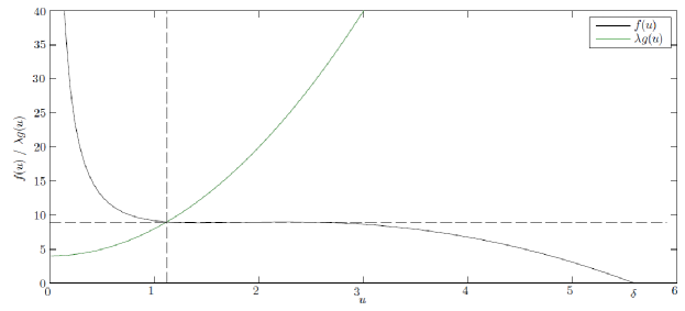
Figure 1: The shape and intersection of functions $f(u)$ and $\lambda g(u)$ for the Lengyel–Epstein reaction–diffusion model (7.3) with maximum $a$.

The solutions of the Lengyel–Epstein model for $a^{2}=\frac{125}{4}$, $b=1$, $c=1$, and $\sigma=0.5$, are depicted in Figures 2 and 3 for the ODE and one–dimensional PDE cases, respectively. The initial data is assumed to be

$$u\left(0\right)=4\text{ and }v\left(0\right)=3,$$

in the ODE case and a slight sinusoidal perturbation is added in the one-dimensional diffusion case

$$u\left(x,0\right)=4+0.2\sin\left(\frac{x}{5}\right)\text{ and }v\left(x,0\right)=3+0.2\cos\left(\frac{x}{5}\right).$$

As expected from our analysis, we observe that the system is aymptotically stable with the equilibrium solution given by (3.2) as

$$\left(u^{\ast},v^{\ast}\right)=\left(\alpha,g\left(\alpha\right)\right)=\left(1.118,2.2499\right).$$

Figure 2: Solutions of the Lengyel–Epstein reaction–diffusion model (7.3) in the ODE case with the chosen parameters.

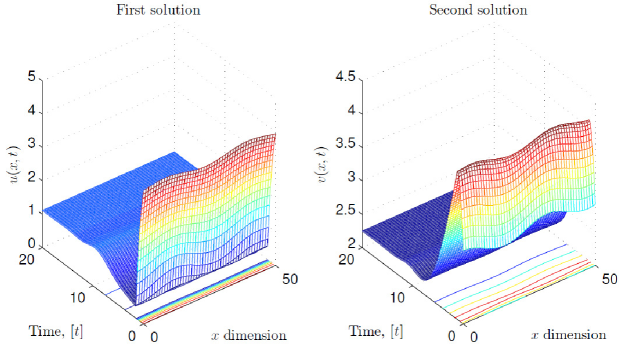
Figure 3: Solutions of the Lenyel–Epstein reaction–diffusion model (7.3) in the one-dimensional diffusion case with the chosen parameters.

7.2 FitzHugh–Nagumo Model

Here, we consider the FitzHugh-Nagumo reaction–diffusion model [15, 7], which represents an excitation system such as a neuron in Human physiology. The system is of the form

$$\left\{\begin{array}[]{l}\frac{\partial u}{\partial t}=d_{1}\Delta u-u^{3}+\left(1+\beta\right)u^{2}-\beta u-v+I\\ \frac{\partial v}{\partial t}=d_{2}\Delta v+\varepsilon u-\varepsilon\gamma v,\end{array}\right.$$ (7.4)

where $u\left(x,t\right)$ and $v\left(x,t\right)$ represent the potential and sodium gating variable in the cell membrane, respectively. The constants $\beta$, $\gamma$, and $\varepsilon$ are assumed to be positive with $0<\beta<1$, $\varepsilon\ll 1$ (accounting for the slow kinetics of the sodium channel). The constant $I$ represents external stimuli. It can be easily observed that this model falls under the general framework proposed in this paper, i.e. system (2.1), with

$$\left\{\begin{array}[]{l}f\left(u\right)=-u^{3}+\left(1+\beta\right)u^{2}-\beta u+I,\\ g\left(u\right)=\frac{u}{\gamma},\\ \varphi\left(u\right)=1,\\ \lambda=1,\\ \sigma=\varepsilon\gamma.\end{array}\right.$$

The constant $\delta$ is the solution of $f(u)=0$ as stated in (2.4), i.e.

$$-u^{3}+\left(1+\beta\right)u^{2}-\beta u+I=0.$$

Note here that $\varphi\left(0\right)\neq 0$ meaning that condition (2.4) is not satisfied. However, as stated in Remark 6, this does not affect the applicability of our results to this case as the inequality (6.1) holds for this particular example. The function $g\left(u\right)$ is clearly increasing and satisfies condition (2.6). We consider, for instance, the case where $\beta=0.139$, $\varepsilon=0.008$, $\gamma=2.54$, and $I=2$. Hence, $\delta=1.7282$. Since, $\lambda=1$ and the functions $f(u)$ and $g(u)$ intersect at a single point as shown in Figure 4, it is safe to say that the FitzHugh–Nagumo system also satisfies condition (2.7). Note that the dynamic range for $u\$is $\left(0,1.7282\right)$ and the unique equilibrium solution of the system as defined by (3.2) is $\left(u^{\ast},v^{\ast}\right)=\left(\alpha,g\left(\alpha\right)\right)=\left(1.5928,0.6273\right)$. Hence, clearly, condition (2.8) is satisfied.

Let us now examine the local asymptotic stability of the equilibrium in the ODE scenario. Differentiating $f\left(u\right)$ and substituting for $\alpha=1.5928$ can easily show that stability conditon (3.3) is satisfied. One thing that remains to be examined is the global asymptotic stability of the system when diffusion is present. It is clear from the shape of $f(u)$ in Figure 4 that it fulfills condition (5.1) over the range $u\in\left(0,\delta\right)$.

The solutions of this particular example were obtained using Matlab simulations and are depicted in Figures 5 and 6 for the ODE and one-dimensional diffusion cases, respectively. Note that in the ODE case, the initial data is assumed to be

$$u\left(0\right)=0.5\text{ and }v\left(0\right)=1.2,$$

whereas in the one-dimensional diffusion case, a slight sinusoidal perturbation is added

$$u\left(x,0\right)=0.5+0.2\sin\left(\frac{x}{5}\right)\text{ and }v\left(x,0\right)=1.2+0.2\cos\left(\frac{x}{5}\right).$$

Clearly, both in the ODE and one-dimensional diffusion cases, the solutions are stable and tend to the equilibrium solution.

Figure 4: The shape and intersection of functions $f(u)$ and $g(u)$ for the FitzHugh-Nagumo reaction–diffusion model.

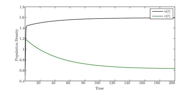
Figure 5: Solutions of the FitzHugh-Nagumo reaction–diffusion model (7.4) in the ODE case with the chosen parameters.

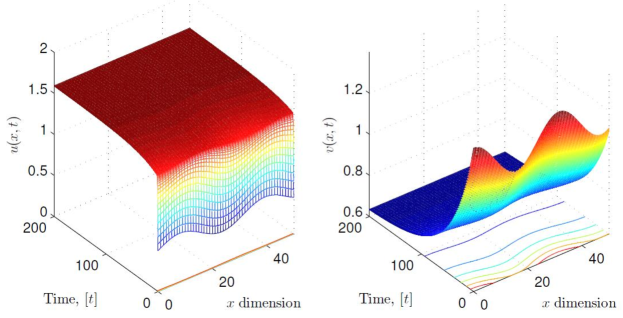
Figure 6: Solutions of the FitzHugh-Nagumo reaction–diffusion model (7.4) in the one-dimensional diffusion case with the chosen parameters.

References

Abdelmalek et al. [2017a] S. Abdelmalek and S.
Bendoukha, On the global asymptotic stability of solutions to a generalized
Lengyel–Epstein system, Nonlinear Analysis: Real World Applications, 35,
397–413, (2017).
Abdelmalek et al. [2017b] S. Abdelmalek, S.
Bendoukha and B. Rebiai, On the stability and non–existence of Turing
patterns for the generalised Lengyel–Epstein model, Math Meth Appl Sci.,
1–11, (2017).
Abdelmalek et al. [to appear] S. Abdelmalek, S.
Bendoukha, B. Rebiai, and M. Kirane, Extended Global Asymptotic Stability
Conditions for a Generalized Reaction–Diffusion System, to appear.
Burton [1985] T.A. Burton, Stability and
periodic solutions of ordinary and functional differential equations,
Academic Press Inc., 1985.
Casten et al. [1977] R. Casten and C.J. Holland,
Stability properties of solutions to systems of reaction–diffusion
equations, SIAM J. Appl. Math. 33 (1977) 353–364.
De Kepper et al. [1990] P. De Kepper, J. Boissonade,
and I. Epstein, Chlorite-iodide reaction: a versatile system for the study
of nonlinear dynamical behavior, J. Phys. Chem. 94, 6525-6536 (1990).
Doelman et al. [2009] A. Doelman, P. van Heijster and
T. J. Kaper, Pulse dynamics in a three component system: existence analysis,
J. Dyn. Diff. Equat., 21(5), 73–115, (2009).
Friedman [1964] A. Friedman, Partial
differential equations of parabolic type, Prentice–Hall: Englewood Cliffs,
1964.
Jang et al. [2004] J. Jang, W. Ni and M. Tang, Global
bifurcation and structure of turing patterns in the 1-D Lengyel–Epstein
model, J. Dyn. Diff. Equ., 16(2), 297–320, (2004).
Lengyel et al. [1991] I. Lengyel and I. R. Epstein,
Modeling of turing structures in the chlorite–iodide–malonic acid–starch
reaction system, Science, 251, 650–652, (1991).
Lengyel et al. [1992] I. Lengyel and I. R. Epstein, A
chemical approach to designing Turing patterns in reaction-diffusion system,
Proc. Nat. Acad. Sci USA, 89, 3977–3979, (1992).
Lisena [2014] B. Lisena, On the global dynamics of the
Lengyel–Epstein system, Appl. Math. &Comp. 249, 67–75, (2014).
Mottoni [1979] P. De Mottoni and F. Rothe, Convergence
to homogeneous equilibrium state for generalized Volterra–Lotka systems
with diffusion, SIAM J. Appl. Math. 37(3), 648–663, (1979).
Ni et al. [2005] W. M. Ni and M. Tang, Turing patterns in
the Lengyel–Epstein system for the CIMA reaction, Trans. Amer. Math. Soc.
357, 3953–3969, (2005).
Oshita et al. [2003] Y. Oshita and I. Ohnishi, Standing
pulse solutions for the FitzHugh-Nagumo equations, Japan J. Indust. Appl.
Math., 20, 101–115, (2003).
Turing [1952] A.Turing, The chemical basis of
morphogenesis, Philos.Trans. R. Soc. Lond. Ser. 237(641), 37–72, (1952).
Wang et al. [2013] L. Wang and H. Zhao, Hopf bifurcation
and turing instability of 2-D Lengyel–Epstein system with
reaction–diffusion terms, Appl. Math. Comput. 219, 9229–9244, (2013).
Weinberger [1975] H. F. Weinberger, Invariant sets for weakly coupled parabolic and elliptic systems, Rend.
Mat. 8, 295–310, (1975).
Yi et al. [2008] F. Yi, J. Wei and J. Shi, Diffusion-driven
instability and bifurcation in the Lengyel–Epstein system, Nonlinear Anal.
RWA 9, 1038–1051, (2008).
Yi et al. [2009] F. Yi, J. Wei and J. Shi, Global
asymptotic behavior of the Lengyel–Epstein reaction–diffusion system,
Appl. Math. Lett. 22, 52–55, (2009).