Efficient construction of tensor ring representations from sampling

Abstract

In this paper we propose an efficient method to compress a high dimensional function into a tensor ring format, based on alternating least-squares (ALS). Since the function has size exponential in $d$ where $d$ is the number of dimensions, we propose efficient sampling scheme to obtain $O(d)$ important samples in order to learn the tensor ring. Furthermore, we devise an initialization method for ALS that allows fast convergence in practice. Numerical examples show that to approximate a function with similar accuracy, the tensor ring format provided by the proposed method has less parameters than tensor-train format and also better respects the structure of the original function.

1 Introduction

Consider a function $f:[n]^{d}\rightarrow\mathbb{R}$ which can be treated as a tensor of size $n^{d}$ ($[n]:=\{1,\ldots,n\}$). In order to store and perform algebraic manipulation of the exponentially sized tensor, typically the tensor $f$ has to be decomposed into various low complexity formats. Most current applications involve the CP [8] or Tucker decomposition [8, 17]. However, the CP decomposition for general tensor is non-unique, whereas the components of Tucker decomposition have exponential size in $d$. The tensor train (TT) [14], better known as the matrix product states (MPS) proposed earlier in physics literature (see e.g. [1, 19, 15]), emerges as an alternative that breaks the curse of dimensionality while avoiding the ill-posedness issue in tensor decomposition. For this format, function compression and evaluation can be done in $O(d)$ complexity. The situation is however unclear when generalizing a TT to a tensor network. Therefore, in this paper, we consider the compression of a black box function $f$ into a tensor ring (TR), i.e., to find 3-tensors $H^{1},\ldots,H^{d}$ such that for $x:=(x_{1},\ldots,x_{d})\in[n]^{d}$

$$f(x_{1},\ldots,x_{d})\approx\operatorname{Tr}\big{(}H^{1}(:,x_{1},:)H^{2}(:,x_{2},:)\cdots H^{d}(:,x_{d},:)\big{)}.$$ (1)

Here $H^{k}\in\mathbb{R}^{r_{k-1}\times n\times r_{k}},r_{k}\leq r$ and we often refer to $(r_{1},\ldots,r_{d})$ as the TR rank. Such type of tensor format is a generalization of the TT format for which $H^{1}\in\mathbb{R}^{1\times n\times r_{1}},H^{d}\in\mathbb{R}^{r_{d-1}\times n\times 1}$. The difference between TR and TT is illustrated in Figure 1 using tensor network diagrams introduced in Section 1.1. Due to the exponential number of entries, typically we do not have access to the entire tensor $f$. Therefore, TR format has to be found based on “interpolation” from $f(\Omega)$ where $\Omega$ is a subset of $[n]^{d}$. For simplicity, in the rest of the note, we assume $r_{1}=r_{2}=\ldots=r_{d}=r$.

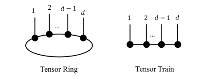
Figure 1: Comparison between a tensor ring and a tensor train.

1.1 Notations

We first summarize the notations used in this note and introduce tensor network diagrams for the ease of presentation. Depending on the context, $f$ is often referred to as a $d$-tensor of size $n^{d}$ (instead of a function). For a $p$-tensor $T$, given two disjoint subsets $\alpha,\beta\subset[p]$ where $\alpha\cup\beta=[p]$, we use

$$T_{\alpha;\beta}$$ (2)

to denote the reshaping of $T$ into a matrix, where the dimensions corresponding to sets $\alpha$ and $\beta$ give rows and columns respectively. Often we need to sample the values of $f$ on a subset of $[n]^{d}$ grid points. Let $\alpha$ and $\beta$ be two groups of dimensions where $\alpha\cup\beta=[d],\alpha\cap\beta=\emptyset$, and $\Omega_{1}$ and $\Omega_{2}$ be some subsampled grid points along the subsets of dimensions $\alpha$ and $\beta$ respectively. We use

$$f(\Omega_{1};\Omega_{2}):=f_{\alpha;\beta}(\Omega_{1}\times\Omega_{2})$$ (3)

to indicate the operation of reshaping $f$ into a matrix, followed by rows and columns subsampling according to $\Omega_{1},\Omega_{2}$. For any vector $x\in[n]^{d}$ and any integer $i$, we let

$$x_{i}:=x_{[(i-1)\bmod d]+1}.$$ (4)

For a $p$-tensor $T$, we define its Frobenius norm as

$$\|T\|_{F}:=\biggl{(}\sum_{i_{1},\ldots,i_{p}}T(i_{1},\ldots,i_{p})^{2}\biggr{)}^{1/2}.$$ (5)

The notation $\text{vec}(A)$ is used to denote the vectorization of a matrix $A$, formed by stacking the columns of $A$ into a vector. For two sets $\alpha,\beta$, we also use the notation

$$\alpha\setminus\beta:=\{i\in\alpha\ |\ i\in\beta^{c}\}$$ (6)

to denote the set difference between $\alpha,\beta$.

In this note, for the convenience of presentation, we use tensor network diagrams to represent tensors and contraction between them. A tensor is represented as a node, where the number of legs of a node indicates the dimensionality of the tensor. For example Figure 2a shows a 3-tensor $A$ and a 4-tensor $B$. When joining edges between two tensors (for example in Figure 2b we join the third leg of $A$ and first leg of $B$), we mean (with the implicit assumption that the dimensions represented by these legs have the same size)

$$\sum_{k}A_{i_{1}i_{2}k}B_{kj_{2}j_{3}j_{4}}.$$ (7)

See the review article [12] for a more complete introduction of tensor network diagrams.

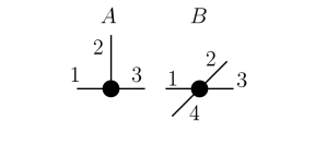
(a)

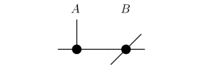
(b)

Figure 2: (a) Tensor diagram for a 3-tensor $A$ and a 4-tensor $B$. (b) Contraction between tensors $A$ and $B$.

1.2 Previous approaches

In this section, we survey previous approaches for compressing a blackbox function into TT or TR. In [13], successive CUR (skeleton) decompositions [6] are applied to find a decomposition of tensor $f$ in TT format. In [4], a similar scheme is applied to find a TR decomposition of the tensor. A crucial step in [4] is to “disentangle” one of the 3-tensors $H^{k}$’s, say $H^{1}$, from the tensor ring. First, $f$ is treated as a matrix where the first dimension of $f$ gives rows, the $2$-nd, $3$-rd, $\ldots,d$-th dimensions of $f$ give columns, i.e., reshaping $f$ to $f_{1;[d]\setminus 1}$. Then CUR decomposition is applied such that

$$f_{1;[d]\setminus 1}=CUR$$ (8)

and the matrix $C\in\mathbb{R}^{n\times r^{2}}$ in the decomposition is regarded as $H^{1}_{2;3,1}$ (the $R$ part in CUR decomposition is never formed due to its exponential size). As noted by the authors in [4], a shortcoming of the method lies in the reshaping of $C$ into $H^{1}$. As in any factorization of low-rank matrix, there is an inherent ambiguity for CUR decomposition in that $CUR=CAA^{-1}UR$ for any invertible matrix $A$. Such ambiguity in determining $H^{1}$ may lead to large tensor-ring rank in the subsequent determination of $H^{2},H^{3}\ldots,H^{d}$. More recently, [22] proposes various ALS-based techniques to determine the TR decomposition of a tensor $f$. However, they only consider the situation where entries of $f$ are fully observed, which limits the applicability of their algorithms to the case with rather small $d$. Moreover, depends on the initialization, ALS can suffer from slow convergence. In [18], ALS is used to determine the TR in a more general setting where only partial observations of the function $f$ are given. In this paper, we further assume the freedom to observe any $O(d)$ entries from the tensor $f$. As we shall see, leveraging such freedom, the complexity of the iterations can be reduced significantly compare to the ALS procedure in [18].

1.3 Our contributions

In this paper, assuming $f$ admits a rank-$r$ TR decomposition, we propose an ALS-based two-phase method to reconstruct the TR when only a few entries of $f$ can be sampled. Here we summarize our contributions.

1. The optimization problem of finding the TR decomposition is non-convex hence requires good initialization in general. We devise method for initializing $H^{1},\ldots,H^{d}$ that helps to resolve the aforementioned ambiguity issues via certain probabilistic assumption on the function $f$.

2. When updating each 3-tensors in the TR, it is infeasible to use all the entries of $f$. We devise a hierarchical strategy to choose the samples of $f$ efficiently via interpolative decomposition. Furthermore, the samples are chosen in a way that makes the per iteration complexity of the ALS linear in $d$.

While we focus in this note the problem of construction tensor ring format, the above proposed strategies can be applied to tensor networks in higher spatial configuration (like PEPS, see e.g., [12]), which will be considered in future works.

The paper is organized as followed. In Section 2 we detail the proposed algorithm. In Section 3, we provide intuition and theoretical guarantess to motivate the proposed initialization procedure, based on certain probabilistic assumption on $f$. In Section 4, we demonstrate the effectiveness of our methods through numerical examples. Finally we conclude the paper in Section 5.

2 Proposed method

In order to find a tensor ring decomposition (1), our overall strategy is to solve the minimization problem

$$\min_{H^{1},\ldots,H^{d}}\sum_{x\in[n]^{d}}\big{(}\operatorname{Tr}(H^{1}[x_{1}]\cdots H^{d}[x_{d}])-f(x_{1},\ldots,x_{d})\big{)}^{2}$$ (9)

where

$$H^{k}[x_{k}]:=H^{k}(:,x_{k},:)\in\mathbb{R}^{r\times r}$$

denotes the $x_{k}$-th slice of the 3-tensor $H^{k}$ along the second dimension. It is computationally infeasible just to set up problem (9), as we need to evaluate $f$ $n^{d}$ times. Therefore, analogous to the matrix or CP-tensor completion problem [3, 21], a “tensor ring completion” problem [18]

$$\min_{H^{1},\ldots,H^{d}}\sum_{x\in\Omega}\big{(}\operatorname{Tr}(H^{1}[x_{1}]\cdots H^{d}[x_{d}])-f(x_{1},\ldots,x_{d})\big{)}^{2}$$ (10)

where $\Omega$ is a subset of $[n]^{d}$ should be solved instead. Since there are a total of $dnr^{2}$ parameters for the tensors $H^{1},\ldots,H^{d}$, there is hope that by observing a small number of entries in $f$ (at least $O(ndr^{2})$), we can obtain the rank-$r$ TR.

A standard approach for solving the minimization problem of the type (10) is via alternating least-squares (ALS). At every iteration of ALS, a particular $H^{k}$ is treated as variable while $H^{l},\l\neq k$ are kept fixed. Then $H^{k}$ is optimized w.r.t. the least-squares cost in (10). More precisely, to determine $H^{k}$, we solve

$$\min_{H^{k}}\sum_{x\in\Omega}\bigl{(}\operatorname{Tr}(H^{k}[x_{k}]C^{x\setminus x_{k}})-f(x)\bigr{)}^{2},$$ (11)

where each coefficient matrix

$$C^{x\setminus x_{k}}:=H^{k+1}[x_{k+1}]\ldots H^{d}[x_{d}]H^{1}[x_{1}]\ldots H^{k-1}[x_{k-1}],\quad x\in\Omega.$$ (12)

By an abuse of notation, we use $x\setminus x_{k}$ to denote the exclusion of $x_{k}$ from the $d$-tuple $x$. As mentioned previously, $|\Omega|$ should be at least $O(ndr^{2})$ in order to determine the tensor ring decomposition. This creates a large computational cost in each iteration of the ALS, as it takes $|\Omega|(d-1)$ (which has $O(d^{2})$ scaling as $|\Omega|$ has size $O(d)$) matrix multiplications just to construct $C^{x\setminus x_{k}}$ for all $x\in\Omega$. When $d$ is large, such quadratic scaling in $d$ for setting up the least-squares problem in each iteration of the ALS is undesirable.

The following simple but crucial observation allows us to gain a further speed up. Although $O(ndr^{2})$ observations of $f$ are required to determine all the components $H^{1},\ldots,H^{d}$, when it comes to determining each individual $H^{k}$ via solving the linear system (11), only $O(nr^{2})$ equations are required for the well-posedness of the linear system. This motivates us to use different $\Omega_{k}$’s each having size $O(nr^{2})$ (with $|\Omega_{1}|+\cdots+|\Omega_{k}|\sim O(ndr^{2})$ ) to determine different $H^{k}$’s in the ALS steps instead of using a fixed set $\Omega$ with size $O(ndr^{2})$ for $H^{k}$’s. If $\Omega_{k}$ is constructed from densely sampling the dimensions near $k$ (where neighborhood is defined according to ring geometry) while sparsely sampling the dimensions far away from $k$, computational savings can be achieved. The specific construction of $\Omega_{k}$ is made precise in Section 2.1. We further remark that if

$$\operatorname{Tr}(H^{k}[x_{k}]C^{x\setminus x_{k}})\approx f(x)$$ (13)

holds with small error for every $x\in[n]^{d}$, then using any $\Omega_{k}\in[n]^{d}$ in place of $\Omega$ in (11) should give similar solutions, as long as (11) is well-posed. Therefore, we solve

$$\min_{H^{k}}\sum_{x\in\Omega_{k}}\bigl{(}\operatorname{Tr}(H^{k}[x_{k}]C^{x\setminus x_{k}})-f(x)\bigr{)}^{2}$$ (14)

instead of (11) in each step of the ALS where the index sets $\Omega_{k}$’s depend on $k$. We note that in practice, a regularization term $\lambda\sigma_{k}\|H^{k}(x_{k})\|_{F}^{2}$ is added to the cost in (14) to reduce numerical instability resulting from potential high condition number of the least-squares problem (14). In all of our experiments, $\lambda$ is set to $10^{-9}$ and $\sigma_{k}$ is the top singular values of the Hessian of the least-squares problem (14). The quality of TR is rather insensitive to the choice of $\lambda$ as long as the value is kept small.

At this point it is clear that there are two issues needed to be addressed. The first issue is concerning the choice of $\Omega_{k},k\in[d]$. Another issue is that non-convex nature of the tensor ring completion problem 10 may cause ALS to converge to a poor local minima. We solve the first issue using a hierarchical sampling strategy. As for the second issue, by making certain probabilistic assumption on $f$, we are able to obtain cheap and intuitive initialization that allows fast convergence. Before moving on, we summarize the full algorithm in Algorithm 1. The steps of Algorithm 1 are further detailed in Section 2.1, 2.2, and 2.3.

Algorithm 1 Alternating least squares

1:

2:Function $f:[n]^{d}\rightarrow\mathbb{R}$.

3:

4:Tensor ring $H^{1},\ldots,H^{d}\in\mathbb{R}^{r\times n\times r}$.

5:Identify the index sets $\Omega_{k}$’s and compute $f(\Omega_{k})$ for each $k\in[d]$ (Section 2.1).

6:Initialize $H^{1},\ldots,H^{d}$ (Section 2.2).

7:Start ALS by solving (14) for each $k\in[d]$ (Section 2.3).

2.1 Constructing $\Omega_{k}$

In this section, we detail the construction of $\Omega_{k}$ for each $k\in[d]$. We first construct an index set $\Omega^{\text{envi}}_{k}\subset[n]^{d-3}$ with fixed size $s$. The elements in $\Omega^{\text{envi}}_{k}$ corresponds to different choices of indices for the $[d]\setminus\{k-1,k,k+1\}$-th dimensions of the function $f$. Then for each of the elements in $\Omega^{\text{envi}}_{k}$, we sample all possible indices from the $(k-1)$-th, $k$-th, $(k+1)$-th dimensions of $f$ to construct $\Omega_{k}$, i.e., letting

$$\Omega_{k}=[n]^{3}\times\Omega^{\text{envi}}_{k}.$$ (15)

We let $|\Omega^{\text{envi}}_{k}|=s$ for all $k$ where $s$ is a constant that does not depend of the dimension $d$. In this case, when determining $C^{x\setminus x_{k}},x\in\Omega_{k}$ in (14), only $O(|\Omega^{\text{envi}}_{k}|d)$ multiplications of $r\times r$ matrices are needed, giving a complexity that is linear in $d$ when setting up the least-squares problem. We want to emphasize that although naively it seems that $O(n^{3})$ samples are needed to construct $\Omega_{k}$ in (15), the $n^{3}$ samples corresponding to each sample in $\Omega^{\text{envi}}_{k}$ can be obtained via applying interpolative decomposition [5] to the $n\times n\times n$ tensor with $O(n)$ observations.

It remains that $\Omega^{\text{envi}}_{k}$’s need to be constructed. There are two criteria we use for constructing $\Omega^{\text{envi}}_{k},k\in[d]$. First, we want the range of $f_{k;[d]\setminus k}(\Omega_{k})$ to be the same as the range of $f_{k;[d]\setminus k}$. Since we expect

$$H^{k}_{2;3,1}[\text{vec}(C^{x\setminus x_{k}})]_{x\in\Omega_{k}}\approx f_{k;[d]\setminus k}(\Omega_{k})$$ (16)

is enforced through the least-squares in (14), the range of $H^{k}_{2;3,1}$ is similar to the range of $f_{k;[d]\setminus k}(\Omega_{k})$. On the other hand, as we expect the optimal $H^{k}$ to satisfy

$$H^{k}_{2;3,1}[\text{vec}(C^{x\setminus x_{k}})]_{x\in[n]^{d}}=f_{k;[d]\setminus k},$$ (17)

for all the entries of $f$, then

$$\text{Range}(f_{k;[d]\setminus k}(\Omega_{k}))=\text{Range}(f_{k;[d]\setminus k}).$$ (18)

Eq. (16) and (18) lead us to require that

$$\text{Range}(f_{k;[d]\setminus k}(\Omega_{k}))=\text{Range}(f_{k;[d]\setminus k}(\Omega_{k})).$$ (19)

Here we emphasize that it is possible to reshape $f(\Omega_{k})$ into a matrix $f_{k;[d]\setminus k}(\Omega_{k})$ as in (16) due to the product structure of $\Omega_{k}$ in (15), where the indices along dimension $k$ are fully sampled. The second criteria is that we require the cost in (14) to approximate the cost in (9).

To meet the first criteria, we propose a hierarchical strategy to determine $\Omega^{\text{envi}}_{k}$ such that $f_{k;[d]\setminus k}(\Omega_{k})$ has large singular values. Assuming $d=3\cdot 2^{L}$ for some natural number $L$, we summarize such strategy in Algorithm 2 (the upward pass) and 3 (the downward pass). The dimensions are divided into groups of size $3\cdot 2^{L-l}$ on each level $l$ for $l=1,\ldots,L$. We emphasize that level $l=1$ corresponds to the coarsest partitioning of the dimensions of the tensor $f$. The purpose of the upward pass is to hierarchically find skeletons $\Theta_{k}^{\text{in},l}$ which represent the $k$-th group of indices, while the downward pass hierarchically constructs representative environment skeletons $\Theta_{k}^{\text{envi},l}$. At each level, the skeletons are found by using rank revealing QR (RRQR) factorization [9].

Algorithm 2 Upward pass

1:

2:Function $f:[n]^{d}\rightarrow\mathbb{R}$, number of skeletons $s$.

3:

4:Skeleton sets $\Theta^{\text{in},l}_{k}$’s

5:Decimate the number of dimensions by clustering every three dimensions. More precisely, for each $k\in[2^{L}]$, let

$$\tilde{\Theta}_{k}^{\text{in},L}:=\{(x_{3k-2},x_{3k-1},x_{3k})\ |\ x_{3k-2},x_{3k-1},x_{3k}\in[n]\}.$$

There are $2^{L}$ index-sets after this step. For each $k\in[2^{L}]$, construct the set of environment skeletons

$$\Theta_{k}^{\text{envi},l}\subset[n]^{d-3},$$ (20)

with $s$ elements either by selecting multi-indices from $[n]^{d-3}$ randomly, or by using the output of Algorithm 3 (when an iteration of upward and downward passes is employed). This step is illustrated in the following figure. (continued on page 2.1.)

6:      (continued from Algorithm 2.)

7:     

8:for $l=L$ to $l=1$

9:      Find the skeletons within each index-set $\tilde{\Theta}_{k}^{\text{in},l}$, $k\in[2^{l}]$ where the elements in each $\tilde{\Theta}_{k}^{\text{in},l}$ are multi-indices of length $3\cdot 2^{L-l}$. Apply RRQR factorization to the matrix $$f(\Theta_{k}^{\text{envi},l};\tilde{\Theta}_{k}^{\text{in},l})\in\mathbb{R}^{s\times|\tilde{\Theta}_{k}^{\text{in},l}|}$$ (21) to select $s$ columns that best resembles the range of $f(\Theta_{k}^{\text{envi},l};\tilde{\Theta}_{k}^{\text{in},l})$. The multi-indices for these $s$ columns form the set $\Theta_{k}^{\text{in},l}$. Store $\Theta_{k}^{\text{in},l}$ for each $k\in[2^{l}]$. This step is illustrated in the following figure, where the thick lines are used to denote the index-sets with size larger than $s$.

10:      If $l>1$, for each $k\in[2^{l-1}]$, construct $$\tilde{\Theta}_{k}^{\text{in},l-1}:=\Theta_{2k-1}^{\text{in},l}\times\Theta_{2k}^{\text{in},l}.$$ (22) Then, sample $s$ elements randomly from $$\prod_{j\in[2^{l}]\setminus\{2k-1,2k\}}\Theta_{j}^{\text{in},l}$$ (23) to form $\Theta_{k}^{\text{envi},l-1}$, or by using the output of Algorithm 3 (when an iteration of upward and downward passes is employed). This step is depicted in the next figure, and again thick lines are used to denote the index-sets with size larger than $d$.

11:      end for

After a full upward-downward pass where RRQR are called $O(d\log d)$ times, $\Theta_{k}^{\text{envi},L}$ with $k\in[2^{L}]$ are obtained. Then another upward pass can be re-initiated. Instead of sampling new $\Theta_{k}^{\text{envi},l}$’s, the stored $\Theta_{k}^{\text{envi},l}$’s in the downward pass are used. Multiple upward-downward passes can be called to further improved these skeletons. Finally, we let

$$\Omega_{3k-1}^{\text{envi}}:=\Theta_{k}^{\text{envi}},\quad k\in[2^{L}].$$ (24)

Observe that we have only obtained $\Omega_{k}^{\text{envi}}$ for $k=2,5,\ldots,d-1$. Therefore, we need to apply upward-downward pass to different groupings of tensor $f$’s dimensions in step (1) of the upward pass. More precisely, we group the dimensions as $(2,3,4),(5,6,7),\ldots,(d-1,d,1)$ and $(d,1,2),(3,4,5),\ldots,(d-3,d-2,d-1)$ when initializing the upward pass to determine $\Omega_{k}^{\text{envi}}$ with $k=3,6,\ldots,d$ and $k=1,4,\ldots,d-2$ respectively.

Algorithm 3 Downward pass

1:

2:Function $f:[n]^{d}\rightarrow\mathbb{R}$, $\Theta^{\text{in},l}_{k}$’s from the upward pass, number of skeletons $s$.

3:

4:Skeletons $\Theta^{\text{envi},l}_{k}$’s

5:Let $\Theta_{1}^{\text{envi},1}=\Theta_{2}^{\text{in},1}$, $\Theta_{2}^{\text{envi},1}=\Theta_{1}^{\text{in},1}$.

6:for $l=2$ to $l=L$

7:      For each $k\in[2^{l}]$, we obtain $\Theta_{k}^{\text{envi},l}$ by applying RRQR factorization to $$f(\Theta_{k}^{\text{in},l};\Theta_{k+1}^{\text{in},l}\times\Theta_{(k+1)/2}^{\text{envi},l-1})$$ (25) or $$f(\Theta_{k}^{\text{in},l};\Theta_{k-1}^{\text{in},l}\times\Theta_{k/2}^{\text{envi},l-1})$$ (26) for odd or even $k$ respectively to obtain $s$ important columns. The multi-indices corresponding to these $s$ columns are used to update $\Theta_{k}^{\text{envi},l}$. The selection of the environment skeletons when $k$ is odd is illustrated in the next figure.

8:end for

Finally, to meet the second criteria that the cost in (14) should approximate the cost in (9), to each $\Omega_{k}^{\text{envi}}$, we add extra samples $x\in[n]^{d-3}$ by sampling $x_{i}$’s uniformly and independently from $[n]$. We typically sample an extra $5s$ samples to each $\Omega_{k}^{\text{envi}}$. This completes the construction for $\Omega_{k}^{\text{envi}}$ ’s and their corresponding $\Omega_{k}$’s in Algorithm 1.

2.2 Initialization

Due to the nonlinearity of the optimization problem (10), it is possible for ALS to get stuck at local minima or saddle points. A good initialization is crucial for the success of ALS. One possibility is to use the “opening” procedure in [4] to obtain each 3-tensors. As mentioned previously, this may suffer ambiguity issue, leading us to consider a different approach. The proposed initialization procedure consists of two steps. First we obtain $H^{k}$’s up to gauges $G^{k}$’s between them (Algorithm 4). Then we solve $d$ least-squares problem to fix the gauges between the $H^{k}$’s (Algorithm 5). More precisely, after Algorithm 4, we want to use $T^{k,C}$ as $H^{k}$. However, as in any factorization, SVD can only determine the factorization of $T^{k,C}$ up to gauge transformations, as shown in Figure 3. Therefore, between $T^{k,C}$ and $T^{k+1,C}$, some appropriate gauge $G^{k}$ has to be inserted (Figure 3).

After gauge fixing, we complete the initialization step in Algorithm 1. Before moving on, we demonstrate the superiority of this initialization v.s. random initialization. In Figure 4 we plot the error between TR and the full function v.s. number of iterations in ALS, when using the proposed initialization and random initialization. By random initialization, we mean the $H^{k}$’s are initialized by sampling their entries independently from the normal distribution. Then ALS is performed on the example detailed in Section 4.3 with $n=3,d=12$. We set the TR rank to be $r=3$. As we can see, after one iteration of ALS, we already obtain $10^{-4}$ error using our proposed method, whereas with random initialization, the convergence of ALS is slower and the solution has a lower accuracy.

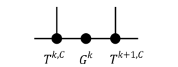
Figure 3: A gauge $G^{k}$ needs to be inserted between $T^{k,C}$ and $T^{k+1,C}$

Figure 4: Plot of convergence of the ALS using both random and the proposed initializations for the numerical example given in Section 4.3 with $n=3,d=12$. The error measure is defined in (40).

Algorithm 4

1:

2:Function $f:[n]^{d}\rightarrow\mathbb{R}$.

3:

4:$T^{k,L}\in\mathbb{R}^{n\times r},T^{k,C}\in\mathbb{R}^{r\times n\times r},T^{k,R}\in\mathbb{R}^{r\times n}$, $k\in[d]$.

5:for $k=1$ to $k=d$

6:      Pick an arbitrary $z\in[n]^{d-3}$ and let $$\Omega_{k}^{\text{ini}}:=\bigl{\{}x\in[n]^{d}\ |\ x_{[d]\setminus\{k-1,k,k+1\}}=z,x_{k-1},x_{k},x_{k+1}\in[n]\bigr{\}}.$$ (27) Define $$T^{k}:=f(\Omega_{k}^{\text{ini}})\in\mathbb{R}^{n\times n\times n}$$ (28) where the first, second and third dimensions of $T^{k}$ correspond to the $(k-1),k,(k+1)$-th dimensions of $f$. Note that we only pick one $z$ in $\Omega^{\text{envi}}_{k}$, which is the key that we can use SVD procedure in the next step and avoid ambiguity in the initialization. The justification of such procedure can be found in Appendix 3.

7:      Now we want to factorize the 3-tensor $T^{k}$ into a tensor train with three nodes using SVD. First treat $T^{k}$ as a matrix by treating the first leg as rows and the second and third legs as columns. Apply a rank-$r$ approximation to $T^{k}$ using SVD: $$T^{k}_{1;2,3}\approx U_{L}\Sigma_{L}V_{L}^{T}.$$ (29) Let $C^{k}\in\mathbb{R}^{r\times n\times n}$ be reshaped from $\Sigma_{L}V_{L}^{T}\in\mathbb{R}^{r\times n^{2}}$.

8:      Treat $C^{k}$ as a matrix by treating the first and second legs as rows and third leg as columns. Apply SVD to obtain a rank-$r$ approximation: $$C^{k}_{1,2;3}\approx U_{R}\Sigma_{R}V_{R}^{T}.$$ (30) Let $\tilde{T}^{k,C}\in\mathbb{R}^{r\times n\times r}$ be reshaped from $U_{R}\Sigma_{R}\in\mathbb{R}^{rn\times r}$.

9:      Let $T^{k,L}:=U_{L}\Sigma_{L}^{1/2}$ and $T^{k,R}:=\Sigma_{R}^{1/2}V_{R}^{T}$. Let $T^{k,C}$ be defined by 3-tensor $T^{k}$ is thus approximated by a tensor train with three tensors $T^{k,L}\in\mathbb{R}^{n\times r},T^{k,C}\in\mathbb{R}^{r\times n\times r},T^{k,R}\in\mathbb{R}^{r\times n}$.

10:end for

Algorithm 5

1:

2:Function $f:[n]^{d}\rightarrow\mathbb{R}$, $T^{k,L},T^{k,C},T^{k,R}$ for $k\in[d]$ from Algorithm 4.

3:

4:Initialization $H^{k},k\in[d]$.

5:for $k=1$ to $k=d$

6:      Pick an arbitrary $z\in[n]^{d-4}$ and let $$\Omega_{k}^{\text{gauge}}:=\bigl{\{}x\in[n]^{d}\ |\ x_{[d]\setminus\{k-1,k,k+1,k+2\}}=z,\,\forall\,x_{k-1},x_{k},x_{k+1},x_{k+2}\in[n]\bigr{\}}$$ (31) and sample $$S^{k}=f(\Omega_{k}^{\text{gauge}})\in\mathbb{R}^{n\times n\times n\times n}.$$ (32)

7:      Solve the least-squares problem $$G^{k}=\underset{G}{\text{argmin}}\ \|L^{k}_{1,2;3}GR^{k}_{1;2,3}-S^{k}_{1,2;3,4}\|_{F}^{2}$$ (33) where $L^{k}$ and $R^{k}$ are defined as

8:      Obtain $H^{k}$:

9:end for

2.3 Alternating least-squares

After constructing $\Omega_{k}$ and initializing $H^{k}$, $k\in[d]$, we start ALS by solving problem (14) at each iteration. This completes Algorithm 1.

When running ALS, sometimes we want to increase the TR-rank to obtain a higher accuracy approximation to the function $f$. In this case, we simply add a row and column of random entries to each $H^{k}$, i.e.

$$H^{k}(:,i,:)\leftarrow\begin{bmatrix}H^{k}(:,i,:)&\epsilon_{1}^{i,k}\\ \epsilon_{2}^{i,k}&1\end{bmatrix},\quad i=1,\ldots,n,\ k=1,\ldots,d,$$ (34)

where each entry of $\epsilon_{1}^{i,k}\in\mathbb{R}^{r\times 1},\epsilon_{2}^{i,k}\in\mathbb{R}^{1\times r}$ is sampled from Gaussian distribution, and continue with the ALS procedure with the new $H^{k}$’s until the error stops decreasing. The variance of each Gaussian random variable is typically set to $10^{-8}$.

3 Motivation of the initialization procedure

In this section, we motivate our initialization procedure in Alg. 4. The main idea is by fixing a random index set, a portion of the ring can be singled out and extracted. To this end, we place the following assumption on the TR $f$.

Assumption 1.

Let the TR $f$ be partitioned into four disjoint regions (Fig 5): Regions $a$, $b$, $c_{1}$ and $c_{2}$ where $a,b,c_{1},c_{2}\subset[d]$. Regions $a,b,c_{1},c_{2}$ contain $L_{a},L_{b},L_{c_{1}},L_{c_{2}}$ number of dimensions respectively where $L_{a}+L_{b}+L_{c_{1}}+L_{c_{2}}=d$. If $L_{a},L_{b}\geq L_{\text{buffer}}$, for any $z\in[n]^{L_{a}+L_{b}}$, the TR $f$ satisfies

$$f(x_{c_{1}},x_{a\cup b},x_{c_{2}})|_{x_{a\cup b}=z}\propto g(x_{c_{1}},x_{a\cup b})|_{x_{a\cup b}=z}h(x_{a\cup b},x_{c_{2}})|_{x_{a\cup b}=z}$$ (35)

for some functions $g,h$. Here “$\propto$” denotes the proportional up to a constant relationship.

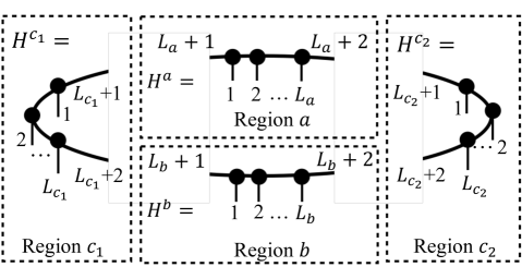
Figure 5: Figure of TR $f$ partitioned into region $a,b,c_{1},c_{2}$.

We note that Assumption 1 holds if $f$ is a non-negative function and admits a Markovian structure. Such functions can arise from Gibbs distribution with energy defined by short-range interactions [20], for example the Ising model.

Next we make certain non-degeneracy assumption on the TR $f$.

Assumption 2.

Any segment $H$ of the TR $f$ (for example $H^{a},H^{b},H^{c_{1}},H^{c_{2}}$ shown in Figure 6), satisfies

$$\operatorname{rank}(H_{L+1,L+2;[L]})=r^{2}$$ (36)

if $L\geq L_{0}$ for some natural number $L_{0}$. In particular, if $L\geq L_{0}$, we assume the condition number of $H_{[L];L+1,L+2}\geq\kappa$ for some $\kappa=1+\delta\kappa$, where $\delta\kappa\geq 0$ is a small parameter.

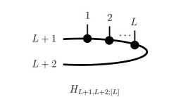
Figure 6: Figure of a segment of TR, denoted as $H$, with $L+2$ dimensions. The $1,\ldots,L$-th dimensions have size $n$, corresponding to outgoing legs of the TR, and the $L+1,L+2$-th dimension are the latent dimensions with size $r$.

Since $H_{L+1,L+2;[L]}\in\mathbb{R}^{r^{2}\times n^{L}}$, it is natural to expect when $n^{L}\geq r^{2}$, $H_{L+1,L+2;[L]}$ is rank $r^{2}$ generically [15].

We now state a proposition that leads us to the intuition behind designing the initialization procedure Algorithm 4.

Proposition 1.

Let

$$s^{1}=e_{i_{1}}\otimes e_{i_{2}}\otimes\cdots\otimes e_{i_{L_{a}}},\quad s^{2}=e_{j_{1}}\otimes e_{j_{2}}\otimes\cdots\otimes e_{j_{L_{b}}}$$ (37)

be any two arbitrary sampling vectors where $\{e_{k}\}_{k=1}^{n}$ is the canonical basis in $\mathbb{R}^{n}$. If $L_{a},L_{b},L_{c_{1}},L_{c_{2}}\geq\max(L_{0},L_{\text{buffer}})$, the two matrices $B^{1},B^{2}\in\mathbb{R}^{r\times r}$ defined in Figure 7 are rank-1.

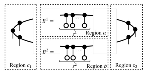
Figure 7: Definition of the matrices $B^{1},B^{2}$ in Proposition 1.

Proof.

Due to Assumption 2, $H^{c_{1}}_{L_{c_{1}}+1,L_{c_{1}}+2;[L_{c_{1}}]}\in\mathbb{R}^{r^{2}\times n^{L_{c_{1}}}}$ and $H^{c_{2}}_{L_{c_{2}}+1,L_{c_{2}}+2;[L_{c_{2}}]}$ $\in\mathbb{R}^{r^{2}\times n^{L_{c_{2}}}}$ defined in Figure 7 are rank-$r^{2}$. Along with the implication of Assumption 1 that

$$\operatorname{rank}\bigl{(}\bigl{(}H^{c_{1}}_{L_{c_{1}}+1,L_{c_{1}}+2;[L_{c_{1}}]}\bigr{)}^{T}B^{1}\otimes B^{2}{H^{c_{2}}_{L_{c_{2}}+1,L_{c_{2}}+2;[L_{c_{2}}]}}\bigr{)}=1,$$ (38)

we get

$$\operatorname{rank}(B^{1}\otimes B^{2})=1.$$ (39)

Since $\operatorname{rank}(B^{1})\operatorname{rank}(B^{2})=\operatorname{rank}(B^{1}\otimes B^{2})=1$, it follows that the rank of $B^{1}$, $B^{2}$ are 1. ∎

The conclusion of Proposition 1 implies that to obtain the segment of TR in region $a$, one simply needs to apply some sampling vector $s^{2}$ in the canonical basis to region $b$ to obtain the configuration in Figure 8 where the vectors $p^{b},q^{b}\in\mathbb{R}^{r}$. Our goal is to extract the nodes in region $a$ as $H^{k}$’s. It is intuitively obvious that one can apply the TT-SVD technique in [13] to extract them. Such technique is indeed used in the proposed initialization procedure where we assume $L_{\text{buffer}}=1,L_{0}=1,L_{a}=1,L_{b}=d-3$. For completeness, in Proposition 2 in the appendix, we formalize the fact that one can use TT-SVD to learn each individual 3-tensor in the TR $f$ up to some gauges. We further provide a perturbation analysis for the case when Markovian-type assumption holds only approximately in Proposition 2.

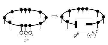
Figure 8: Applying a sampling vector $s^{2}$ in the canonical basis to region $b$ gives the TT.

4 Numerical results

In this section, we present numerical results on the proposed method for tensor ring decomposition. We calculate the error between the obtained tensor ring decomposition and function $f$ as:

$$E=\sqrt{\frac{\sum_{x\in\Omega}\big{(}\operatorname{Tr}(H^{1}[x_{1}]\cdots H^{d}[x_{d}])-f(x_{1},\ldots,x_{d})\big{)}^{2}}{\sum_{x\in\Omega}f(x_{1},\ldots,x_{d})^{2}}}.$$ (40)

Whenever it is feasible, we let $\Omega=[n]^{d}$. Otherwise, we subsample $\Omega$ from $[n]^{d}$ at random: For every $x\in\Omega$, $x_{i}$ is drawn from $[n]$ uniformly at random. If the dimensionality of $f$ is large, we simply sample $\Omega$ from $[n]^{d}$ at random. For the proposed algorithm, we also measure the error on the entries sampled for learning TR as:

$$E_{\text{skeleton}}=\sqrt{\frac{\sum_{x\in\cup_{k}\Omega_{k}}\big{(}\operatorname{Tr}(H^{1}[x_{1}]\cdots H^{d}[x_{d}])-f(x_{1},\ldots,x_{d})\big{)}^{2}}{\sum_{x\in\cup_{k}\Omega_{k}}f(x_{1},\ldots,x_{d})^{2}}}.$$ (41)

In the experiments, we compare our method, denoted as TR-ALS+, with TR-ALS proposed in [18]. In [18], the cost in (9) is minimized using ALS where (11) is solved for each $k$ in an alternating fashion. Although [18] proposed an SVD based initialization approach similar to the recursive SVD algorithm for TT [13], this method has exponential complexity in $d$. Therefore the comparison with such an initialization is omitted and we use randomized intialization for TR-ALS. As we shall see, TR-ALS+ is generally an order of magnitude faster than TR-ALS, due to the special structure of the samples. For each experiment we run both TR-ALS and TR-ALS+ for five times and report the median accuracy. For TR-ALS, we often have to use less samples such that the running time is not excessively long (recall that TR-ALS has $O(d^{2})$ complexity per iteration). We also compare ourselves with the DMRG-Cross algorithm [16] (which gives a TT). As a method that is based on interpolative decomposition, DMRG-Cross is able to obtain high quality approximation if we allow a large TT-rank representation. Since we obtain the TR based on ALS optimization, the accuracy may not be comparable to DMRG-Cross. What we want to emphasize here is that if the given situation only requires moderate accuracy, our method could give a more economical representation than TT obtained from DMRG-Cross. To convey this message, we set the accuracy of DMRG-Cross so that it matches the accuracy of our proposed TR-ALS.

4.1 Example 1: A toy example

We first compress the function

$$f(x_{1},\ldots,x_{d})=\frac{1}{\sqrt{1+x_{1}^{2}+\ldots+x_{d}^{2}}},\quad x_{k}\in[0,1]$$ (42)

considered in [4] into a tensor ring. In this example, we let $s=4$ (recall that $s$ is the size of $\Omega_{k}^{\text{envi}}$) in TR-ALS+. The number of samples we can afford to use for TR-ALS is less than TR-ALS+ due to the excessively long running time since each iteration of TR-ALS has a complexity scaling of $O(d^{2})$. In this example, although sometimes TR-ALS+ has lower accuracy than TR-ALS, the running time of TR-ALS+ is significantly shorter. In particular, for the case when $d=12$, TR-ALS fails to converge using the same amount of samples as TR-ALS+. Both TR-ALS+ and TR-ALS give TR with tensor components with smaller sizes than TT. The error $E$ reported for the case of $d=12$ is obtained from sampling $10^{5}$ entires of the tensor $f$.

Setting	Format	Rank $(r_{1},\ldots,r_{d})$	$E_{\text{skeleton}}$	$E$	$\frac{\text{Number of observations}}{n^{d}}$	Run Time (s)
$d=6,n=10$	TR-ALS+	(3,3,3,3,3,3)	2.3e-03	6.3e-04	1.8e-01	4.7
	TR-ALS	(3,3,3,3,3,3)	4.3e-05	4.5e-05	2.8e-02	1360
	TT	(5,5,5,5,5,1)	-	1.2e-04	-	2.4
$d=6,n=20$	TR-ALS+	(3,3,3,3,3,3)	5.1e-04	9.4e-05	2.1e-02	24
	TR-ALS	(3,3,3,3,3,3)	5.0e-05	5.4e-05	8.2e-04	2757
	TT	(5,5,6,5,5,1)	-	6.8e-05	-	7.1
$d=12,n=5$	TR-ALS+	(3,3,3,3,3,3   3,3,3,3,3,3)	7.1e-04	5.9e-04	1.7e-04	28
	TT-ALS	(3,3,3,3,3,3   3,3,3,3,3,3)	0.97	0.97	1.7e-04	3132
	TT	(5,6,6,6,6,6   6,6,5,5,5,1)	-	2.2e-05	-	2.9

Table 1: Results for Example 1. $n$ corresponds to the number of uniform grid points on $[0,1]$ for each $x_{k}$. The tuple $(r_{1},\ldots,r_{d})$ indicates the rank of the learnt TR and TT. $E_{\text{skeleton}}$ is computed on the samples used for learning the TR.

4.2 Example 2: Ising spin glass

In this example, we demosntrate the advantage of TR-ALS+ in compressing high-dimensional function arising from many-body physics, the traditional field where TT or MPS is extensively used [1, 19]. We consider compressing the free energy of Ising spin glass with a ring geometry:

$$f(J_{1},\ldots,J_{d})=-\frac{1}{\beta}\log\bigg{[}\operatorname{Tr}\bigg{(}\prod_{i=1}^{d}\begin{bmatrix}e^{\beta J_{i}}&e^{-\beta J_{i}}\\ e^{-\beta J_{i}}&e^{\beta J_{i}}\end{bmatrix}\bigg{)}\bigg{]}.$$ (43)

We let $\beta=10$, and $J_{i}\in\{-2.5,-1.5,1,2\},i\in[d]$. This corresponds to Ising model with temperature of about 0.1K. We let the number of environment samples $s=5$. When computing the error $E$ for the case of $d=24$, due to the size of $f$, we simply sub-sample $10^{5}$ entries of $f$ where $J_{i}$’s are sampled independently and uniformly from $\{-2.5,-1.5,1,2\}$. For $d=12$, the solution obtained by TR-ALS+ is superior due to the initialization procedure. We see that in both $d=12,24$ cases, the running time of TR-ALS is much longer compare to TR-ALS+.

Setting	Format	Rank $(r_{1},\ldots,r_{d})$	$E_{\text{skeleton}}$	$E$	$\frac{\text{Number of observations}}{n^{d}}$	Run Time (s)
$d=12,n=4$	TR-ALS+	(4,4,4,4,4,4   4,4,4,4,4,4)	3.9e-03	3.8e-03	1.6e-02	7
	TR-ALS	(4,4,4,4,4,4   4,4,4,4,4,4)	4.4e-02	5.2e-02	1.6e-02	994
	TT	(6,7,7,7,7,7   7,7,7,6,4,1)	-	4.2e-03	-	2.8
$d=24,n=4$	TR-ALS+	(3,3,3,3,3,3  3,3,3,3,3,3   3,3,3,3,3,3   3,3,3,3,3,3)	4.8e-03	2.7e-03	1.6e-10	19
	TR -ALS	-	-	-	1.6e-10	-
	TT	(6,8,8,8,6,6  6,6,6,6,7,6  5,6,6,6,6,7   7,6,6,6,4,1)	-	3.7e-03	-	9.3

Table 2: Results for Example 2. Learning the free energy of Ising spin glass.

4.3 Example 3: Parametric elliptic partial differential equation (PDE)

In this section, we demonstrate the performance of our method in solving parametric PDE. We are interested in solving elliptic equation with random coefficients

$$\frac{\partial}{\partial x}a(x)\bigg{(}\frac{\partial}{\partial x}u(x)+1\bigg{)}=0,\quad x\in[0,1]$$ (44)

subject to periodic boundary condition, where $a(\cdot)$ is a random field. In particular, we want to parameterize the effective conductance function

$$A_{\text{eff}}(a(\cdot)):=\int_{[0,1]}a(x)\bigg{(}\frac{\partial}{\partial x}u(x)+1\bigg{)}^{2}dx$$ (45)

as a TR. By discretizing the domain into $d$ segments and assuming $a(x)=\sum_{i=1}^{d}a_{i}\chi_{i}(x)$, where each $a_{i}\in[1,2,3]$ and $\chi_{i}$’s being step functions on uniform intervals on $[0,1]$, we determine $A_{\text{eff}}(a_{1},\ldots,a_{d})$ as a TR. In this case, the effective coefficients have an analytic solution

$$A_{\text{eff}}(a_{1},\ldots,a_{d})=\bigg{(}\frac{1}{d}\sum_{i=1}^{d}a_{i}\bigg{)}^{-1}$$ (46)

and we use this formula to generate samples to learn the TR. For this example, we pick $s=4$. The results are reported in Table 3. When computing $E$ with $d=24$, again $10^{5}$ entries of $f$ are subsampled where $a_{i}$’s are sampled independently and uniformly from $\{1,2,3\}$. We note that although in this situation, there is an analytic formula for the function we want to learn as a TR, we foresee further usages of our method when solving parametric PDE with periodic boundary condition, where there is no analytic formula for the physical quantity of interest (for example for the cases considered in [10]).

Setting	Format	Rank $(r_{1},\ldots,r_{d})$	$E_{\text{skeleton}}$	$E$	$\frac{\text{Number of observations}}{n^{d}}$	Run Time (s)
$d=12,n=3$	TR-ALS+	(3,3,3,3,3,3   3,3,3,3,3,3)	1.1e-05	1.1e-05	1.4e-02	22
	TR-ALS	(3,3,3,3,3,3   3,3,3,3,3,3)	5.7e-06	6.8e-06	1.4e-02	1414
	TT	(5,5,5,5,5,5   5,5,5,3,3,1)	-	2.5e-05	-	0.76
$d=24,n=3$	TR-ALS+	(3,3,3,3,3,3  3,3,3,3,3,3   3,3,3,3,3,3   3,3,3,3,3,3)	2.6e-05	2.8e-05	5.5e-06	47
	TR-ALS	-	-	-	5.5e-06	-
	TT	(5,5,5,5,5,5  5,5,5,5,5,5  5,5,5,5,5,5   5,5,5,3,3,1)	-	1.7e-05	-	1.5

Table 3: Results for Example 3. Solving parametric elliptic PDE.

5 Conclusion

In this paper, we propose method for learning a TR representation based on ALS. Since the problem of determining a TR is a non-convex optimization problem, we propose an initialization strategy that helps the convergence of ALS. Furthermore, since using the entire tensor $f$ in the ALS is infeasible, we propose an efficient hierarchical sampling method to identify the important samples. Our method provides a more economical representation of the tensor $f$ than TT-format. As for future works, we plan to investigate the performance of the algorithms for quantum systems. One difficulty is that the Assumption 1 (Appendix 3) for the proposed initialization procedure does not in general hold for quantum systems with short-range interactions. Instead, a natural assumption for a quantum state exhibiting a tensor-ring format representation is the exponential correlation decay [7, 2]. The design of efficient algorithms to determine the TR representation under such assumption is left for future works. Another natural direction is to extend the proposed method to tensor networks in higher spatial dimension, which we shall also explore in the future.

Appendix A Stability of initialization

In this section, we analyze the stability of the proposed initialization procedure, where we relax Assumption 1 to approximate Markovianity.

Assumption 3.

Let

$$\Omega_{z}:=\bigl{\{}(x_{c_{1}},x_{a\cup b},x_{c_{2}})\mid x_{c_{1}}\in[n]^{L_{c_{1}}},x_{c_{2}}\in[n]^{L_{c_{2}}},x_{a\cup b}=z\bigr{\}}$$ (47)

for some given $z\in[n]^{L_{a}+L_{b}}$. For any $z\in[n]^{L_{a}+L_{b}}$, we assume

$$\frac{\|f(\Omega_{z})_{c_{1};a\cup b\cup c_{2}}\|_{2}^{2}}{\|f(\Omega_{z})_{c_{1};a\cup b\cup c_{2}}\|_{F}^{2}}\geq\alpha.$$ (48)

for some $0<\alpha\leq 1$ if $L_{a},L_{b}\geq L_{\text{buffer}}$.

This assumption is a relaxation of Assumption 1. Indeed, if (48) holds for $\alpha=1$, it implies that $f(\Omega_{z})_{c_{1};a\cup b\cup c_{2}}$ is rank $1$. Under the Assumption 3, we want to show that using Algorithm 4, one can extract $H^{k}$’s approximately. The final result is stated in Proposition 2, obtained via the next few lemmas. In particular, we show that when the condition number $\kappa$ of the tensor ring components (defined in Lemma 1) satisfies $\kappa=1$, as $\alpha\rightarrow 1$, the approximation error goes to $0$. In the first lemma, we show that $B^{1},B^{2}$ defined in Figure 7 are approximately rank-1.

Lemma 1.

Let $H^{c_{1}},H^{c_{2}},B^{1},B^{2}$ be defined according to Figure 5 and 7, where the sampling vectors $s^{1},s^{2}$ are defined in Proposition 1. If $L_{c_{1}},L_{c_{2}},L_{a},L_{b}\geq\max(L_{0},L_{\text{buffer}})$, then

$$\frac{\|B^{1}\|_{2}^{2}}{\|B^{1}\|_{F}^{2}},\frac{\|B^{2}\|_{2}^{2}}{\|B^{2}\|_{F}^{2}}\geq\frac{\alpha}{\kappa^{4}}.$$ (49)

Proof.

By Assumption 3,

$$\alpha \leq\frac{\bigl{\lVert}\bigl{(}H^{c_{1}}_{L_{c_{1}}+1,L_{c_{1}}+2;[L_{c_{1}}]}\bigr{)}^{T}B^{1}\otimes B^{2}{H^{c_{2}}_{L_{c_{2}}+1,L_{c_{2}}+2;[L_{c_{2}}]}}\bigr{\rVert}_{2}^{2}}{\bigl{\lVert}\bigl{(}H^{c_{1}}_{L_{c_{1}}+1,L_{c_{1}}+2;[L_{c_{1}}]}\bigr{)}^{T}B^{1}\otimes B^{2}{H^{c_{2}}_{L_{c_{2}}+1,L_{c_{2}}+2;[L_{c_{2}}]}}\bigr{\rVert}_{F}^{2}}$$ (50)

$$\leq\kappa_{c_{1}}^{2}\kappa_{c_{2}}^{2}\frac{\|B^{1}\otimes B^{2}\|_{2}^{2}}{\|B^{1}\otimes B^{2}\|_{F}^{2}}$$ (51)

$$=\kappa_{c_{1}}^{2}\kappa_{c_{2}}^{2}\frac{\|B^{1}\|_{2}^{2}}{\|B^{1}\|_{F}^{2}}\frac{\|B^{2}\|_{2}^{2}}{\|B^{2}\|_{F}^{2}},$$ (52)

where $\kappa_{c_{1}},\kappa_{c_{2}}\leq\kappa$ are condition numbers of $H^{c_{1}}_{L_{c_{1}}+1,L_{c_{1}}+2;[L_{c_{1}}]}$ and $H^{c_{2}}_{L_{c_{2}}+1,L_{c_{2}}+2;[L_{c_{2}}]}$ respectively. ∎

Let $p^{b}({q^{b}})^{T}$ be the best rank-1 approximation to $B^{2}$. Before registering the next corollary, we define $H^{[d]\setminus b}$ and $\tilde{H}^{[d]\setminus a}$ in Figure 9.

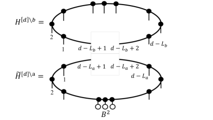
Figure 9: Definition of $H^{[d]\setminus b}$ and $\tilde{H}^{[d]\setminus a}$.

Corollary 1.

Under the assumptions of Lemma 1, for any sampling operator $s^{2}$ defined in Proposition 1,

$$\frac{\|H^{[d]\setminus b}_{[d-L_{b}];d-L_{b}+1,d-L_{b}+2}\text{vec}(p^{b}({q^{b}})^{T})-f_{[d]\setminus b;b}s^{2}\|_{2}^{2}}{\|f_{[d]\setminus b;b}s^{2}\|_{F}^{2}}\leq\kappa^{2}(1-\frac{\alpha}{\kappa^{4}}).$$ (53)

Proof.

Lemma 1 implies

$$\frac{\|H^{b}_{L_{b}+1,L_{b}+2;[L_{b}]}s^{2}-\text{vec}(p^{b}({q^{b}})^{T})\|_{2}^{2}}{\|H^{b}_{L_{b}+1,L_{b}+2;[L_{b}]}s^{2}\|_{2}^{2}}$$ (54)

$$\qquad=\frac{\|B^{2}-p^{b}({q^{b}})^{T}\|_{F}^{2}}{\|B^{2}\|_{F}^{2}}=\frac{\|B^{2}\|_{F}^{2}-\|p^{b}({q^{b}})^{T}\|_{F}^{2}}{\|B^{2}\|_{F}^{2}}\leq 1-\frac{\alpha}{\kappa^{4}}.$$ (55)

Then

$$\frac{\|H^{[d]\setminus b}_{[d-L_{b}];d-L_{b}+1,d-L_{b}+2}\text{vec}(p^{b}({q^{b}})^{T})-f_{[d]\setminus b;b}s^{2}\|_{2}^{2}}{\|f_{[d]\setminus b;b}s^{2}\|_{2}^{2}}$$ (56)

$$\qquad\leq\frac{\|H^{[d]\setminus b}_{[d-L_{b}];d-L_{b}+1,d-L_{b}+2}\|_{2}^{2}\|H^{b}_{L_{b}+1,L_{b}+2;[L_{b}]}s^{2}-\text{vec}(p^{b}({q^{b}})^{T})\|_{2}^{2}}{\|H^{[d]\setminus b}_{[d-L_{b}];d-L_{b}+1,d-L_{b}+2}H^{b}_{L_{b}+1,L_{b}+2;[L_{b}]}s^{2}\|_{2}^{2}}$$ (57)

$$\qquad\leq\kappa_{[d]\setminus b}^{2}\frac{\|H^{b}_{L_{b}+1,L_{b}+2;[L_{b}]}s^{2}-\text{vec}(p^{b}({q^{b}})^{T})\|_{2}^{2}}{\|H^{b}_{L_{b}+1,L_{b}+2;[L_{b}]}s^{2}\|_{2}^{2}}$$ (58)

where $\kappa_{[d]\setminus b}^{2}$ is the condition number of $H^{[d]\setminus b}_{[d-L_{b}];d-L_{b}+1,d-L_{b}+2}$. Recall that $H^{b}$ is defined in Figure 5. ∎

This corollary states that the situation in Figure 8 holds approximately. More precisely, let $T,\hat{T}\in\mathbb{R}^{n^{d-L_{b}}}$ be defined as

$$T:=H^{[d]\setminus b}_{[d-L_{b}];d-L_{b}+1,d-L_{b}+2}\text{vec}(p^{b}({q^{b}})^{T}),\ \hat{T}:=f_{[d]\setminus b;b}s^{2}$$ (59)

respectively, as demonstrated in Figure 10a, where $p^{b},q^{b}$ appear in Corollary 1. Corollary 1 implies

$$T=\hat{T}+E,\quad\frac{\|E\|_{F}^{2}}{\|\hat{T}\|_{F}^{2}}\leq\kappa^{2}(1-\frac{\alpha}{\kappa^{4}}).$$ (60)

In the following, we want to show that we can approximately extract the $H^{k}$’s in region $a$. For this, we need to take the right-inverses of $\tilde{H}^{c_{1}}_{L_{c_{1}}+1;[L_{c_{1}}]}$ and $\tilde{H}^{c_{2}}_{L_{c_{2}}+1;[L_{c_{2}}]}$, defined in Figure 10b. This requires a singular value lower bound, provided by the next lemma.

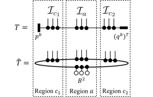
(a)

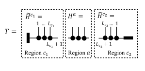
(b)

Figure 10: (a) Definition of $T$ and $\hat{T}$. The dimensions in region $a,c_{1},c_{2}$ are group into $\mathcal{I}_{a},\mathcal{I}_{c_{1}},\mathcal{I}_{c_{2}}$ respectively for the tensors $T$ and $\hat{T}$. (b) Individual components of $T$.

Lemma 2.

Let $\sigma_{k}:\mathbb{R}^{m_{1}\times m_{2}}\rightarrow\mathbb{R}$ be a function that extracts the $k-th$ singular value of a $m_{1}\times m_{2}$ matrix. Then

$$\frac{\sigma_{r}(\tilde{H}^{c_{1}}_{L_{c_{1}}+1;[L_{c_{1}}]})^{2}\sigma_{r}(\tilde{H}^{c_{2}}_{L_{c_{2}}+1;[L_{c_{2}}]})^{2}}{\|\tilde{H}^{[d]\setminus a}_{d-L_{a}+1,d-L_{a}+2;[d-L_{a}]}\|_{2}^{2}}\geq\frac{1}{\kappa^{6}}-\frac{2\sqrt{r}}{\kappa^{2}}\sqrt{1-\frac{\alpha}{\kappa^{4}}}$$ (61)

assuming

$$\frac{1}{\kappa^{4}}-2\sqrt{r}\sqrt{1-\frac{\alpha}{\kappa^{4}}}\geq 0.$$ (62)

Proof.

Firstly,

$$\frac{\sigma_{r^{2}}(T_{\mathcal{I}_{a};\mathcal{I}_{c_{1}}\mathcal{I}_{c_{2}}})^{2}}{\|\hat{T}_{\mathcal{I}_{a};\mathcal{I}_{c_{1}},\mathcal{I}_{c_{2}}}\|_{2}^{2}} \leq\frac{\|H^{a}_{[L_{a}];L_{a}+1,L_{a}+2}\|_{2}^{2}\sigma_{r^{2}}(\tilde{H}^{c_{1}}_{L_{c_{1}}+1;[L_{c_{1}}]}\otimes\tilde{H}^{c_{2}}_{L_{c_{2}}+1;[L_{c_{2}}]})^{2}}{\|\hat{T}_{\mathcal{I}_{a};\mathcal{I}_{c_{1}},\mathcal{I}_{c_{2}}}\|_{2}^{2}}$$ (63)

$$=\frac{\|H^{a}_{[L_{a}];L_{a}+1,L_{a}+2}\|_{2}^{2}\sigma_{r}(\tilde{H}^{c_{1}}_{L_{c_{1}}+1;[L_{c_{1}}]})^{2}\sigma_{r}(\tilde{H}^{c_{2}}_{L_{c_{2}}+1;[L_{c_{2}}]})^{2}}{\|H^{a}_{[L_{a}];L_{a}+1,L_{a}+2}\tilde{H}^{[d]\setminus a}_{d-L_{a}+1,d-L_{a}+2;[d-L_{a}]}\|_{2}^{2}}$$ (64)

$$\leq\frac{\|H^{a}_{[L_{a}];L_{a}+1,L_{a}+2}\|_{2}^{2}\sigma_{r}(\tilde{H}^{c_{1}}_{L_{c_{1}}+1;[L_{c_{1}}]})^{2}\sigma_{r}(\tilde{H}^{c_{2}}_{L_{c_{2}}+1;[L_{c_{2}}]})^{2}}{\sigma_{r^{2}}(H^{a}_{[L_{a}];L_{a}+1,L_{a}+2})^{2}\|\tilde{H}^{[d]\setminus a}_{d-L_{a}+1,d-L_{a}+2;[d-L_{a}]}\|_{2}^{2}}$$ (65)

$$\leq\kappa^{2}\frac{\sigma_{r}(\tilde{H}^{c_{1}}_{L_{c_{1}}+1;[L_{c_{1}}]})^{2}\sigma_{r}(\tilde{H}^{c_{2}}_{L_{c_{2}}+1;[L_{c_{2}}]})^{2}}{\|\tilde{H}^{[d]\setminus a}_{d-L_{a}+1,d-L_{a}+2;[d-L_{a}]}\|_{2}^{2}}\,.$$ (66)

The equality follows from

$$\hat{T}_{\mathcal{I}_{a};\mathcal{I}_{c_{1}},\mathcal{I}_{c_{2}}}=H^{a}_{[L_{a}];L_{a}+1,L_{a}+2}\tilde{H}^{[d]\setminus a}_{d-L_{a}+1,d-L_{a}+2;[d-L_{a}]},$$

which follows from (59), and the definition of $\tilde{H}^{[d]\setminus a}$ in Figure 9.

Observe that

$$\frac{\sigma_{r^{2}}(T_{\mathcal{I}_{a};\mathcal{I}_{c_{1}},\mathcal{I}_{c_{2}}})^{2}}{\|\hat{T}_{\mathcal{I}_{a};\mathcal{I}_{c_{1}},\mathcal{I}_{c_{2}}}\|_{2}^{2}} \geq\frac{\sigma_{r^{2}}(\hat{T}_{\mathcal{I}_{a};\mathcal{I}_{c_{1}},\mathcal{I}_{c_{2}}})^{2}-2\|E\|_{F}\sigma_{r^{2}}(\hat{T}_{\mathcal{I}_{a};\mathcal{I}_{c_{1}},\mathcal{I}_{c_{2}}})+\|E\|_{F}^{2}}{\|\hat{T}_{\mathcal{I}_{a};\mathcal{I}_{c_{1}},\mathcal{I}_{c_{2}}}\|_{2}^{2}}$$ (67)

$$\geq\frac{\sigma_{r^{2}}(\hat{T}_{\mathcal{I}_{a};\mathcal{I}_{c_{1}},\mathcal{I}_{c_{2}}})^{2}}{\|\hat{T}_{\mathcal{I}_{a};\mathcal{I}_{c_{1}},\mathcal{I}_{c_{2}}}\|_{2}^{2}}-\frac{2\|E\|_{F}\sigma_{r^{2}}(\hat{T}_{\mathcal{I}_{a};\mathcal{I}_{c_{1}},\mathcal{I}_{c_{2}}})}{\|\hat{T}_{\mathcal{I}_{a};\mathcal{I}_{c_{1}},\mathcal{I}_{c_{2}}}\|_{2}^{2}}$$ (68)

$$\geq\frac{\sigma_{r^{2}}(H^{a}_{[L_{a}];L_{a}+1,L_{a}+2})^{2}\sigma_{r^{2}}(\tilde{H}^{[d]\setminus a}_{d-L_{a}+1,d-L_{a}+2;[d-L_{a}]})^{2}}{\|H^{a}_{[L_{a}];L_{a}+1,L_{a}+2}\|_{2}^{2}\|\tilde{H}^{[d]\setminus a}_{d-L_{a}+1,d-L_{a}+2;[d-L_{a}]}\|_{2}^{2}}$$ (69)

$$\qquad-\frac{2\|E\|_{F}\sigma_{r^{2}}(\hat{T}_{\mathcal{I}_{a};\mathcal{I}_{c_{1}},\mathcal{I}_{c_{2}}})}{\|\hat{T}_{\mathcal{I}_{a};\mathcal{I}_{c_{1}},\mathcal{I}_{c_{2}}}\|_{2}^{2}}$$ (70)

$$\geq\frac{1}{\kappa^{4}}-\frac{2\|E\|_{F}\sigma_{r^{2}}(\hat{T}_{\mathcal{I}_{a};\mathcal{I}_{c_{1}},\mathcal{I}_{c_{2}}})}{\|\hat{T}_{\mathcal{I}_{a};\mathcal{I}_{c_{1}},\mathcal{I}_{c_{2}}}\|_{2}^{2}}$$ (71)

$$\geq\frac{1}{\kappa^{4}}-\frac{2\sqrt{r}\sigma_{r^{2}}(\hat{T}_{\mathcal{I}_{a};\mathcal{I}_{c_{1}},\mathcal{I}_{c_{2}}})\|E\|_{F}}{\|\hat{T}_{\mathcal{I}_{a};\mathcal{I}_{c_{1}},\mathcal{I}_{c_{2}}}\|_{2}\|\hat{T}_{\mathcal{I}_{a};\mathcal{I}_{c_{1}},\mathcal{I}_{c_{2}}}\|_{F}}$$ (72)

$$\geq\frac{1}{\kappa^{4}}-2\sqrt{r}\sqrt{1-\frac{\alpha}{\kappa^{4}}},$$ (73)

we established the claim. The first inequality regarding perturbation of singular values follows from theorem by Mirsky [11]:

$$\bigl{\lvert}\sigma_{r^{2}}(T_{\mathcal{I}_{a};\mathcal{I}_{c_{1}},\mathcal{I}_{c_{2}}})-\sigma_{r^{2}}(\hat{T}_{\mathcal{I}_{a};\mathcal{I}_{c_{1}},\mathcal{I}_{c_{2}}})\bigr{\rvert}\leq\|E\|_{2}\leq\|E\|_{F},$$ (74)

and assuming $\|E\|_{F}\leq\sigma_{r^{2}}(\hat{T}_{\mathcal{I}_{a};\mathcal{I}_{c_{1}},\mathcal{I}_{c_{2}}})$ . Such assumption holds when demanding the lower bound in (67) to be nonnegative, i.e.

$$\frac{\sigma_{r^{2}}(\hat{T}_{\mathcal{I}_{a};\mathcal{I}_{c_{1}},\mathcal{I}_{c_{2}}})^{2}}{\|\hat{T}_{\mathcal{I}_{a};\mathcal{I}_{c_{1}},\mathcal{I}_{c_{2}}}\|_{2}^{2}}-\frac{2\|E\|_{F}\sigma_{r^{2}}(\hat{T}_{\mathcal{I}_{a};\mathcal{I}_{c_{1}},\mathcal{I}_{c_{2}}})}{\|\hat{T}_{\mathcal{I}_{a};\mathcal{I}_{c_{1}},\mathcal{I}_{c_{2}}}\|_{2}^{2}}\geq\frac{1}{\kappa^{4}}-2\sqrt{r}\sqrt{1-\frac{\alpha}{\kappa^{4}}}\geq 0$$ (75)

The last inequality follows from Corollary 1. ∎

In the next lemma, we prove that when applying Algorithm 4 to $\hat{T}$, where $\hat{T}$ is treated as a 3-tensor formed from grouping the dimensions in each of set $\mathcal{I}_{a},\mathcal{I}_{c_{1}}\mathcal{I}_{c_{2}}$, gives close approximation to $\hat{T}$.

Lemma 3.

Let

$$\Pi_{1} :=\bigl{\{}Y\ |\ Y=XX^{T},X\in\mathbb{R}^{n^{L_{c_{1}}}\times r},\ X^{T}X=I\bigr{\}},$$ (76)

$$\Pi_{2} :=\bigl{\{}Y\ |\ Y=XX^{T},X\in\mathbb{R}^{n^{L_{c_{2}}}\times r},\ X^{T}X=I\bigr{\}},$$ (77)

where $I$ is the identity matrix. Let $P_{1}^{*}\in\Pi_{1}$ be the best rank-$r$ projection for $\hat{T}_{\mathcal{I}_{c_{2}}\mathcal{I}_{a};\mathcal{I}_{c_{1}}}$ such that $\hat{T}_{\mathcal{I}_{c_{2}}\mathcal{I}_{a};\mathcal{I}_{c_{1}}}P_{1}^{*}\approx\hat{T}_{\mathcal{I}_{c_{2}}\mathcal{I}_{a};\mathcal{I}_{c_{1}}}$ in Frobenius-norm, and

$$P_{2}^{*}=\min_{P_{2}\in\Pi_{2}}\|(\hat{T}_{\mathcal{I}_{a};\mathcal{I}_{c_{1}}\mathcal{I}_{c_{2}}}(I\otimes P_{2})-\hat{T}_{\mathcal{I}_{a};\mathcal{I}_{c_{1}}\mathcal{I}_{c_{2}}})(P_{1}^{*}\otimes I)\|_{F}^{2}.$$

Then

$$\|\hat{T}_{\mathcal{I}_{a};\mathcal{I}_{c_{1}}\mathcal{I}_{c_{2}}}(I\otimes P_{2}^{*})(P_{1}^{*}\otimes I)-\hat{T}_{\mathcal{I}_{a};\mathcal{I}_{c_{1}}\mathcal{I}_{c_{2}}}\|_{F}^{2}\leq 2\|E\|_{F}^{2}.$$ (78)

Proof.

To simplify the notations, let $\tilde{T}_{\mathcal{I}_{a};\mathcal{I}_{c_{1}}\mathcal{I}_{c_{2}}}:=\hat{T}_{\mathcal{I}_{a};\mathcal{I}_{c_{1}}\mathcal{I}_{c_{2}}}(I\otimes P_{2})$. Then

$$\min_{P_{2}\in\Pi_{2}}\|\hat{T}_{\mathcal{I}_{a};\mathcal{I}_{c_{1}}\mathcal{I}_{c_{2}}}(I\otimes P_{2})(P_{1}^{*}\otimes I)-\hat{T}_{\mathcal{I}_{a};\mathcal{I}_{c_{1}}\mathcal{I}_{c_{2}}}\|_{F}^{2}$$ (79)

$$= \min_{P_{2}\in\Pi_{2}}\|(\tilde{T}_{\mathcal{I}_{a};\mathcal{I}_{c_{1}}\mathcal{I}_{c_{2}}}-\hat{T}_{\mathcal{I}_{a};\mathcal{I}_{c_{1}}\mathcal{I}_{c_{2}}}+\hat{T}_{\mathcal{I}_{a};\mathcal{I}_{c_{1}}\mathcal{I}_{c_{2}}})(P_{1}^{*}\otimes I)-\hat{T}_{\mathcal{I}_{a};\mathcal{I}_{c_{1}}\mathcal{I}_{c_{2}}}\|_{F}^{2}$$ (80)

$$= \min_{P_{2}\in\Pi_{2}}\|\hat{T}_{\mathcal{I}_{a};\mathcal{I}_{c_{1}}\mathcal{I}_{c_{2}}}(I-P_{1}^{*}\otimes I)\|_{F}^{2}+\|(\tilde{T}_{\mathcal{I}_{a};\mathcal{I}_{c_{1}}\mathcal{I}_{c_{2}}}-\hat{T}_{\mathcal{I}_{a};\mathcal{I}_{c_{1}}\mathcal{I}_{c_{2}}})(P_{1}^{*}\otimes I)\|_{F}^{2}$$ (81)

$$\leq \min_{P_{2}\in\Pi_{2}}\|\hat{T}_{\mathcal{I}_{a};\mathcal{I}_{c_{1}}\mathcal{I}_{c_{2}}}(I-P_{1}^{*}\otimes I)\|_{F}^{2}+\|\tilde{T}_{\mathcal{I}_{a};\mathcal{I}_{c_{1}}\mathcal{I}_{c_{2}}}-\hat{T}_{\mathcal{I}_{a};\mathcal{I}_{c_{1}}\mathcal{I}_{c_{2}}}\|_{F}^{2}$$ (82)

$$= \min_{P_{2}\in\Pi_{2}}\|\hat{T}_{\mathcal{I}_{a};\mathcal{I}_{c_{1}}\mathcal{I}_{c_{2}}}(I-P_{1}^{*}\otimes I)\|_{F}^{2}+\|\hat{T}_{\mathcal{I}_{a};\mathcal{I}_{c_{1}}\mathcal{I}_{c_{2}}}(I-I\otimes P_{2})\|_{F}^{2}.$$ (83)

The inequality comes from the fact that $P_{1}^{*}\otimes I$ is a projection matrix. Next,

$$\|\hat{T}_{\mathcal{I}_{a};\mathcal{I}_{c_{1}}\mathcal{I}_{c_{2}}}(I-P_{1}^{*}\otimes I)\|_{F}^{2}+\min_{P_{2}\in\Pi_{2}}\|\hat{T}_{\mathcal{I}_{a};\mathcal{I}_{c_{1}}\mathcal{I}_{c_{2}}}(I-I\otimes P_{2})\|_{F}^{2}\\ =\min_{P_{1}\in\Pi_{1}}\|\hat{T}_{\mathcal{I}_{a};\mathcal{I}_{c_{1}}\mathcal{I}_{c_{2}}}(I-P_{1}\otimes I)\|_{F}^{2}+\min_{P_{2}\in\Pi_{2}}\|\hat{T}_{\mathcal{I}_{a};\mathcal{I}_{c_{1}}\mathcal{I}_{c_{2}}}(I-I\otimes P_{2})\|_{F}^{2}\\ \leq\|E\|_{F}^{2}+\|E\|_{F}^{2}\leq 2\|E\|_{F}^{2},$$ (84)

and we can conclude the lemma. The equality comes from the definition of $P_{1}^{*}$, whereas the inequality is due to the facts that $P_{1},P_{2}$ are rank-$r$ projectors, and there exists $T$ such that $\hat{T}=T-E$ where $\text{rank}(T_{\mathcal{I}_{c_{1}}\mathcal{I}_{a};\mathcal{I}_{c_{2}}})$, $\text{rank}(T_{\mathcal{I}_{c_{1}};\mathcal{I}_{a}\mathcal{I}_{c_{2}}})$ $\leq r$. ∎

We are ready to state the final proposition.

Proposition 2.

Let

$$\hat{\vphantom{\rule{1.0pt}{5.71527pt}}\smash{\hat{T}}}_{\mathcal{I}_{a};\mathcal{I}_{c_{1}}\mathcal{I}_{c_{2}}}:=\hat{T}_{\mathcal{I}_{a};\mathcal{I}_{c_{1}}\mathcal{I}_{c_{2}}}(I\otimes P_{2}^{*})(P_{1}^{*}\otimes I)$$ (85)

where $P_{1}^{*},P_{2}^{*}$ are defined in Lemma 3. Then

$$\frac{\|H^{a}_{[L_{a}];L_{a}+1,L_{a}+2}-\hat{\vphantom{\rule{1.0pt}{5.71527pt}}\smash{\hat{T}}}_{\mathcal{I}_{a};\mathcal{I}_{c_{1}}\mathcal{I}_{c_{2}}}(\tilde{H}^{c_{1}}_{L_{c_{1}}+1;[L_{c_{1}}]}\otimes\tilde{H}^{c_{2}}_{L_{c_{2}}+1;[L_{c_{2}}]})^{\dagger}\|_{F}^{2}}{\|H^{a}_{[L_{a}];L_{a}+1,L_{a}+2}\|_{F}^{2}}\leq\frac{(1+\sqrt{2})^{2}\kappa^{4}(1-\frac{\alpha}{\kappa^{4}})}{\frac{1}{\kappa^{4}}-2\sqrt{r}\sqrt{1-\frac{\alpha}{\kappa^{4}}}},$$ (86)

where “$\dagger$” is used to denote the pseudo-inverse of a matrix, if the upper bound is positive. When $\kappa=1+\delta\kappa$ and $\alpha=1-\delta\alpha$ where $\delta\kappa,\delta\alpha\geq 0$ are small parameters, we have

$$\frac{\|H^{a}_{[L_{a}];L_{a}+1,L_{a}+2}-\hat{\vphantom{\rule{1.0pt}{5.71527pt}}\smash{\hat{T}}}_{\mathcal{I}_{a};\mathcal{I}_{c_{1}}\mathcal{I}_{c_{2}}}(\tilde{H}^{c_{1}}_{L_{c_{1}}+1;[L_{c_{1}}]}\otimes\tilde{H}^{c_{2}}_{L_{c_{2}}+1;[L_{c_{2}}]})^{\dagger}\|_{F}^{2}}{\|H^{a}_{[L_{a}];L_{a}+1,L_{a}+2}\|_{F}^{2}}\leq O(\delta\alpha+4\delta\kappa).$$ (87)

Proof.

From Lemma 3 and (60), we get

$$\|\hat{\vphantom{\rule{1.0pt}{5.71527pt}}\smash{\hat{T}}}_{\mathcal{I}_{a};\mathcal{I}_{c_{1}}\mathcal{I}_{c_{2}}}-T_{\mathcal{I}_{a};\mathcal{I}_{c_{1}}\mathcal{I}_{c_{2}}}\|_{F}$$ (88)

$$= \|\hat{T}_{\mathcal{I}_{a};\mathcal{I}_{c_{1}}\mathcal{I}_{c_{2}}}(I\otimes P_{2}^{*})(P_{1}^{*}\otimes I)-T_{\mathcal{I}_{a};\mathcal{I}_{c_{1}}\mathcal{I}_{c_{2}}}\|_{F}$$ (89)

$$\leq \|\hat{T}_{\mathcal{I}_{a};\mathcal{I}_{c_{1}}\mathcal{I}_{c_{2}}}(I\otimes P_{2}^{*})(P_{1}^{*}\otimes I)-\hat{T}_{\mathcal{I}_{a};\mathcal{I}_{c_{1}}\mathcal{I}_{c_{2}}}\|_{F}+\|\hat{T}_{\mathcal{I}_{a};\mathcal{I}_{c_{1}}\mathcal{I}_{c_{2}}}-T_{\mathcal{I}_{a};\mathcal{I}_{c_{1}}\mathcal{I}_{c_{2}}}\|_{F}$$ (90)

$$\leq (1+\sqrt{2})\|E\|_{F}.$$ (91)

Recall that

$$H^{a}_{[L_{a}];L_{a}+1,L_{a}+2}=T_{\mathcal{I}_{a};\mathcal{I}_{c_{1}},\mathcal{I}_{c_{2}}}(\tilde{H}^{c_{1}}_{L_{c_{1}}+1;[L_{c_{1}}]}\otimes\tilde{H}^{c_{2}}_{L_{c_{2}}+1;[L_{c_{2}}]})^{\dagger},$$ (92)

where the existence of a full-rank pseudo-inverse is guaranteed by the singular value lower bound in Lemma 2, we have

$$\frac{\|H^{a}_{[L_{a}];L_{a}+1,L_{a}+2}-\hat{\vphantom{\rule{1.0pt}{5.71527pt}}\smash{\hat{T}}}_{\mathcal{I}_{a};\mathcal{I}_{c_{1}},\mathcal{I}_{c_{2}}}(\tilde{H}^{c_{1}}_{L_{c_{1}}+1;[L_{c_{1}}]}\otimes\tilde{H}^{c_{2}}_{L_{c_{2}}+1;[L_{c_{2}}]})^{\dagger}\|_{F}^{2}}{\|H^{a}_{[L_{a}];L_{a}+1,L_{a}+2}\|_{F}^{2}}$$ (93)

$$\leq \frac{(1+\sqrt{2})^{2}\|E\|_{F}^{2}\|(\tilde{H}^{c_{1}}_{L_{c_{1}}+1;[L_{c_{1}}]}\otimes\tilde{H}^{c_{2}}_{L_{c_{2}}+1;[L_{c_{2}}]})^{\dagger}\|_{2}^{2}}{\|H^{a}_{[L_{a}];L_{a}+1,L_{a}+2}\|_{F}^{2}}$$ (94)

$$\leq \frac{(1+\sqrt{2})^{2}\|E\|_{F}^{2}}{\sigma_{r}(\tilde{H}^{c_{1}}_{L_{c_{1}}+1;[L_{c_{1}}]})^{2}\sigma_{r}(\tilde{H}^{c_{2}}_{L_{c_{2}}+1;[L_{c_{2}}]})^{2}\|H^{a}_{[L_{a}];L_{a}+1,L_{a}+2}\|_{F}^{2}}$$ (95)

$$= \frac{(1+\sqrt{2})^{2}\|\hat{T}\|_{F}^{2}}{\sigma_{r}(\tilde{H}^{c_{1}}_{L_{c_{1}}+1;[L_{c_{1}}]})^{2}\sigma_{r}(\tilde{H}^{c_{2}}_{L_{c_{2}}+1;[L_{c_{2}}]})^{2}\|H^{a}_{[L_{a}];L_{a}+1,L_{a}+2}\|_{F}^{2}}\frac{\|E\|_{F}^{2}}{\|\hat{T}\|_{F}^{2}}$$ (96)

$$\leq \frac{(1+\sqrt{2})^{2}\|\tilde{H}^{[d]\setminus a}_{d-L_{a}+1,d-L_{a}+2;[d-L_{a}]}\|_{2}^{2}}{\sigma_{r}(\tilde{H}^{c_{1}}_{L_{c_{1}}+1;[L_{c_{1}}]})^{2}\sigma_{r}(\tilde{H}^{c_{2}}_{L_{c_{2}}+1;[L_{c_{2}}]})^{2}}\frac{\|E\|_{F}^{2}}{\|\hat{T}\|_{F}^{2}}$$ (97)

$$\leq \frac{(1+\sqrt{2})^{2}}{\frac{1}{\kappa^{6}}-\frac{2\sqrt{r}}{\kappa^{2}}\sqrt{1-\frac{\alpha}{\kappa^{4}}}}\kappa^{2}(1-\frac{\alpha}{\kappa^{4}}).$$ (98)

The first inequality follows from (91) and (92), and the last inequality follows from Corollary 1 and Lemma 2. ∎

When $L_{a}=L_{c_{1}}=L_{c_{2}}=1$, applying Algorithm 4 to $\hat{T}$ results $\hat{\vphantom{\rule{1.0pt}{5.71527pt}}\smash{\hat{T}}}$ (represented by the tensors $T^{a,L},T^{a,C}$ and $T^{a,R}$). Therefore, this proposition essentially implies $T^{a,C}$ approximates $H^{a}$ up to gauge transformation.

References

- [1] I. Affleck, T. Kennedy, E. H. Lieb, and H. Tasaki, Valence bond ground states in isotropic quantum antiferromagnets, Comm. Math. Phys. 115 (1988), 477–528.
- [2] F. G. S. L. Brandao and M. Horodecki, Exponential decay of correlations implies area law, Commun. Math. Phys. 333 (2015), 761–798.
- [3] Emmanuel J Candès and Benjamin Recht, Exact matrix completion via convex optimization, Foundations of Computational mathematics 9 (2009), no. 6, 717.
- [4] Mike Espig, Kishore Kumar Naraparaju, and Jan Schneider, A note on tensor chain approximation, Computing and Visualization in Science 15 (2012), no. 6, 331–344.
- [5] Shmuel Friedland, V Mehrmann, A Miedlar, and M Nkengla, Fast low rank approximations of matrices and tensors, Electronic Journal of Linear Algebra 22 (2011), no. 1, 67.
- [6] Feliks Ruvimovich Gantmacher and Joel Lee Brenner, Applications of the theory of matrices, Courier Corporation, 2005.
- [7] M. B. Hastings and T. Koma, Spectral gap and exponential decay of correlations, Commun. Math. Phys. 265 (2006), 781–804.
- [8] Frank L Hitchcock, The expression of a tensor or a polyadic as a sum of products, Journal of Mathematics and Physics 6 (1927), no. 1-4, 164–189.
- [9] Yoo Pyo Hong and C-T Pan, Rank-revealing QR factorizations and the singular value decomposition, Mathematics of Computation 58 (1992), no. 197, 213–232.
- [10] Yuehaw Khoo, Jianfeng Lu, and Lexing Ying, Solving parametric PDE problems with artificial neural networks, 2017, preprint, arXiv:1707.03351.
- [11] Leon Mirsky, Symmetric gauge functions and unitarily invariant norms, The quarterly journal of mathematics 11 (1960), no. 1, 50–59.
- [12] R. Orus, A practical introduction to tensor networks: Matrix product states and projected entangled pair states, Ann. Phys. 349 (2013), 117–158.
- [13] Ivan Oseledets and Eugene Tyrtyshnikov, TT-Cross approximation for multidimensional arrays, Linear Algebra and its Applications 432 (2010), no. 1, 70–88.
- [14] Ivan V Oseledets, Tensor-train decomposition, SIAM Journal on Scientific Computing 33 (2011), no. 5, 2295–2317.
- [15] David Perez-Garcia, Frank Verstraete, Michael M Wolf, and J Ignacio Cirac, Matrix product state representations, Quantum Inf. Comput. 7 (2007), 401.
- [16] Dmitry Savostyanov and Ivan Oseledets, Fast adaptive interpolation of multi-dimensional arrays in tensor train format, Multidimensional (nD) Systems (nDs), 2011 7th International Workshop on, IEEE, 2011, pp. 1–8.
- [17] Ledyard R Tucker, Some mathematical notes on three-mode factor analysis, Psychometrika 31 (1966), no. 3, 279–311.
- [18] Wenqi Wang, Vaneet Aggarwal, and Shuchin Aeron, Efficient low rank tensor ring completion, Proceedings of the IEEE International Conference on Computer Vision, 2017, pp. 5697–5705.
- [19] Steven R White, Density matrix formulation for quantum renormalization groups, Physical review letters 69 (1992), no. 19, 2863.
- [20] M. M. Wolf, F. Verstraete, M. B. Hastings, and J. I. Cirac, Area laws in quantum systems: Mutual information and correlations, Phys. Rev. Lett. 100 (2008), 070502.
- [21] Ming Yuan and Cun-Hui Zhang, On tensor completion via nuclear norm minimization, Foundations of Computational Mathematics 16 (2016), no. 4, 1031–1068.
- [22] Qibin Zhao, Guoxu Zhou, Shengli Xie, Liqing Zhang, and Andrzej Cichocki, Tensor ring decomposition, arXiv preprint arXiv:1606.05535 (2016).