Deep Active Learning over the Long Tail
Abstract
This paper is concerned with pool-based active learning for deep neural networks. Motivated by coreset dataset compression ideas, we present a novel active learning algorithm that queries consecutive points from the pool using farthest-first traversals in the space of neural activation over a representation layer. We show consistent and overwhelming improvement in sample complexity over passive learning (random sampling) for three datasets: MNIST, CIFAR-10, and CIFAR-100. In addition, our algorithm outperforms the traditional uncertainty sampling technique (obtained using softmax activations), and we identify cases where uncertainty sampling is only slightly better than random sampling.
1 Introduction and Related Work
Active learning provides a learning algorithm with some control over the learning process, potentially leading to significantly more efficient learning in terms of labeling efforts (Cohn et al., 1994). The key question in active learning is how many label requests are sufficient to train a classifier to a specified accuracy, a quantity known as label complexity (Hanneke, 2013). Theoretically, there are instances where effective active learning can achieve ‘exponential speedup’ – roughly meaning that to achieve excess-risk, the dominating factor in the active learner’s label complexity will be rather than (or in the agnostic case) (Balcan et al., 2006). This huge asymptotic potential saving is tantalizing. With the growth of deep and large neural models that are hungry for huge labeled samples, the importance and need for effective active learning techniques is only growing. Unfortunately, the literature on active learning in deep neural networks is extremely sparse, and the few existing works fall short of providing viable active learning solutions for practical applications.
One major obstacle in applying any active learning algorithm without prior knowledge, is the need to select its hyper-parameters on the fly, while acquiring labeled samples. This is a challenging task, especially in the early stages of the active learning session while the currently available labeled dataset is still small and extremely biased. Many seminal works on active learning avoided dealing with this hard problem altogether, by intentionally selecting a good set of hyper-parameters based on ‘prior knowledge’ (Tong & Koller, 2001; Baram et al., 2004; Gal et al., 2017). The few studies that included hyper-parameter selection within the active learning process do not report significant improvements of the active learning algorithm over random sampling (“passive learning”); see, e.g. Huang et al. (2015). In the context of deep nets, because of the extreme sensitivity of large neural nets to a variety of hyper-parameters (such as learning rates, initialization schemes, regularization techniques, and the architecture itself), this hyper-parameter selection trap is expected to be much more severe. We believe that this inherent difficulty hinders further developments of deep active networks, at least within the traditional setting of active learning.
In this paper we consider a “long-tail” variant of pool-based active learning. In our variant, a (deep) model has already been initially trained to achieve reasonable accuracy. Then, in a sequence of phases, and based on budgetary constraints (or accuracy improvement requirements), additional labels are sought to increase the model’s accuracy. In each phase, a specified number of samples to be labeled are to be selected from a given large pool of unlabeled samples. At this point, an active learning algorithm is applied and its performance should improve upon random sampling of the points from the pool, uniformly at random (i.e., passive learning). Thus, this active setting variant essentially differs from the standard pool-based setting (Tong & Koller, 2001) in its starting point. In our setting, we don’t expect to gain anything during the early stages of the active learning. On the contrary, we are willing to invest on random sampling at the beginning in order to gain much later when improving the model, over the “long tail” of the training process. Active learning, thus, becomes the means to expedite model improvements. We show that our setting mitigates the hyper-parameter selection challenge, stabilizes the active performance (which is typically extremely noisy and unreliable in early active stages), and overall, allows for practical deep active learning with quite impressive sample complexity speedups, compared to passive learning.
Our long-tail active learning setting and our new active learning algorithm (see Section 3) are inspired by a novel study on dataset compression described below, whereby the goal is to take a given deep model trained on some dataset and find, in hindsight, a subset of training samples that will generate a similar performance (when training the model over the compressed dataset). We show that activation levels in the representation layer provide sufficient information to compress CIFAR-10 to 50% of its original size while compromising only 1.5% in accuracy. This level of dataset compression has not been previously reported. The ability to compress a dataset using representation-layer activations of an already trained model motivates both our active learning setting and our new active learning algorithm itself.
There is a rich literature on active learning, which is beyond the scope of this paper. For a sample of the classic and some modern works, see (Cohn et al., 1994; Freund et al., 1993; Tong & Koller, 2001; Baram et al., 2004; Balcan & Long, 2013; Huang et al., 2015). For a comprehensive summary of the theory of (disagreement-based) active learning, and its relationship to selective prediction, see (Hanneke, 2013; El-Yaniv & Wiener, 2012). A recurring idea in (pool-based) active learning is that of uncertainty sampling, which means that unlabeled pool of points are prioritized by model uncertainty, and the most uncertain points should be queried first. Applications of uncertainty sampling depend on the model. In neural networks uncertainty of a point is approximated by the network’s Softmax Response (SR) activation recorded for , which reflects distance from the decision boundary. In the context of deep nets, Gal et al. (2017) presented active learning algorithms based on a clever Monte-Carlo dropout technique and applied them on the MNIST dataset using a relatively small network, and for detecting skin cancer from images by fine-tuning a pre-trained VGG16 architecture. Wang et al. (2016) applied the well-known softmax response (SR) idea supplemented with pseudo-labeling (self-labeling of highly confident points) for actively learning the ‘cross-age-celebrity’ dataset and Caltech-256, using a deep architecture that was pre-trained over Imagenet. Zhou et al. (2013) constructed a deep architecture based on a restricted Boltzmann machine (RBM) to actively learn sentiment categorization. Their active learning algorithm relied on pre-training the RBM over a large unlabeled dataset, and their querying function used SR. All these works achieved reasonable active learning performance by exploiting prior knowledge, which significantly helped to surmount the hyper-parameter and model selection obstacles. In this sense, these works strongly support and motivate the setting we propose here with “late” starting of the active queries. In addition, these works heavily relied on the softmax response idea, which was slightly improved upon by Gal et al. (2017) using their Monte-Carlo dropout technique, which can be viewed as consolidating several independent applications of softmax response.
1.1 Problem Setting
Consider a standard supervised learning problem defined in terms of a feature space , a label space , and an underlying distribution , where , . Based on a labeled training set of training samples, the goal is to select a prediction function , , so as to minimize the risk , where is a given loss function.
In our “long-tail” active learning setting, we assume that a “reasonable” function has already been trained using supervised learning over the random sample . We are also given a pool of unlabeled samples from . We now consider two problem variants:
-
1.
Budget-constrained: Given a budget for labeling, actively select from , unlabeled samples and request their label to obtain a labeled set . Then use to train whose risk is the smallest possible.
-
2.
Error-reduction: Given an , select from the minimal number of samples, whose labels will be requested so as create the labeled sample . Use to find such that . We note that should be sufficiently small to enable this task to be accomplished (and we cannot know in advance if the required error-reduction is achievable).
The performance of the “passive” solution for both these variants will be the natural benchmark for any active method. The passive solution is obtained by training using a training set created by random (uniform) sampling of points in . For example, in the budget-constrained variant, the passive learning algorithm samples a subset of points from the given points uniformly at random to create .
Finally, we decompose a deep neural model as , where consists of the first part of the network from the input layer until (and including) a higher representation layer, and represent the final layers. In this work we consider the representation layer as the second last layer and is the classifier in the last layer.
2 Motivation: Compression Schemes for Deep Learning
A coreset is a sub-sample of a dataset, which can be used as a proxy for the full set. The idea in the study of coresets (Phillips, 2016) is to use them to approximate the full dataset such that the output of an algorithm over the coreset will be qualitatively similar to its output over the full dataset (with respect to some cost function). Coresets can be used to create efficient approximation algorithms by running the same algorithm on a small fraction of the input data. Many coresets ideas are based on computational geometry. The goal of the present work was to find a compression scheme for a given deep neural model. Inspired by techniques used in coresets, we experimented with the farthest-first (FF) traversal, also known as the Gonzalez algorithm (Gonzalez, 1985), which can be used to obtain an efficient 2-approximation algorithm for the -center clustering problem (Hochbaum, 1996). Given a set of points in a metric space, its FF traversal is constructed by taking the first point arbitrarily, then take the farthest point from as the next point, and in subsequent steps always greedily choose the point farthest away from any of the points already chosen.
When dealing with complex input signals such as images or sound, it makes little sense to consider the input space itself. A natural observation is that in a trained deep model, there are representation layers that create manifolds on which semantically similar objects tend to be closer to each other. Thus, the geometry over spaces induced by these layers can be useful for creating coresets.
The basic FF idea thus gives rise to the following compression algorithm, which we call farthest-first compression (FF-Comp). Consider a multi-class classification problem with classes. Given a training set, , we train a deep neural model , where represents the the entire network excluding the last layer (see Section 1.1). We construct coresets, one for each class, using FF traversals over the spaces . Formally, suppose we are creating the coresets , . Denoting , for a non-empty , the next labeled point, , to be added to , is
| (1) | |||||
The resulting compression algorithm is given in Algorithm 1. This algorithm essentially selects up to points from in a “stratified” manner.
To evaluate the performance of the resulting compression, we retrain the same architecture using , and assess its test error over an independent labeled set. Applying FF-Comp over the CIFAR-10 dataset, we obtained 50% compression with a degrading test error of only 1.5% (93.23% accuracy before, and 91.73% after). While this might seem to be a very impressive compression, comparing it to the 3.1% accuracy reduction obtained by a random 50% compression is somewhat disappointing. It turns out, however, that the required random sub-sampling rate that will lead to 91.73% accuracy over the test set (as in the more clever FF compression) is 64%, which amounts to an additional 7,000 labeled training points to match the compression performance. Viewed from an active learning perspective, this is a large saving that can potentially be exploited. This result motivates the construction of a new active learning algorithm based on FF traversals over the representation level of a trained model within the proposed “long tail” setting of active learning.
3 Deep Active Learning with Coresets
The compression result of Section 2 motivates an active learning algorithm whose querying function operates by computing coresets. We consider the long-tail active setting of Section 1.1 whereby we already have a trained deep model that was trained over . We also assume we have access to itself, as well as to a pool of unlabeled points. At each stage in the active session we have a labeled training set and an unlabeled pool (initially, and ) and we would like to select additional points from , request their label, and then re-train over (which is the union of with the newly acquiried labeled points).
We would like to apply the same coreset principle as in the FF-Comp compression scheme. However, note that in the active game, the pool is unlabeled and we cannot stratify the queried points. Algorithm 2 provides the pseudo-code for our active learning algorithm, for which we intentionally formulated only the basic principle without applying various potential improvements such as pseudo labeling (which can be used to apply stratification or to enrich the labeled training set at each iteration). The algorithm receives as input the initial classifier , its training set , the unlabeled pool , and a batch size , defined to be the number of extra pool points to be queried at each round.
.
4 Experiments
In this section we report on the results of several experiments. In each experiment we compare the performance of our FF-Active algorithm to that of the traditional softmax response (SR) method (uncertainty sampling) and to Random (passive learning). We experimented with three standard datasets: MNIST, CIFAR-10, and CIFAR-100. These experiments indicate that FF-Active has significant advantage over Random, and that it is better than SR. We also present an experiment over a synthetic expansion of CIFAR-100, which highlights a more challenging scenario for SR.
4.1 MNIST
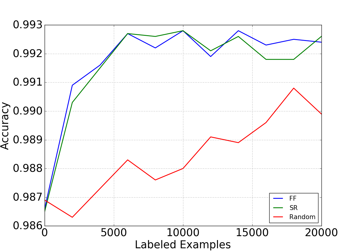
We begin by testing FF-Active over the MNIST dataset for which we trained a network similar to LeNet (LeCun et al., 1998), whose architecture contains two convolutional layers, one fully-connected hidden layer and a softmax layer. We used Adam as the optimization algorithm. MNIST consists of 10 classes of images of hand-written digits, and contains 60,000 labeled examples. We performed the initial training over a labeled set, , containing 10,000 images sampled uniformly at random from the entire set. The remaining 50,000 images were taken to be the unlabeled pool . The active session consists of rounds where in each one, each active learning algorithm selected an additional 2000 points from the pool according to its querying function. The resulting learning curves of FF-Active, SR and Random are presented in Figure 1. It is evident that FF-Active quickly extracted much of the relevant information in after 8000 additional labeled points. Random, on the other hand, did not achieve this performance level even after 20,000 additional labeled queries. In this dataset the performance of SR is indistinguishable from that of FF-Active.
4.2 CIFAR-10
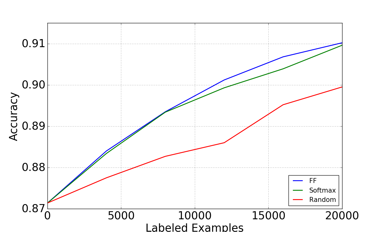
For the CIFAR-10 dataset (Krizhevsky & Hinton, 2009) we employed the VGG-16 architecture (Simonyan & Zisserman, 2014). We trained the model for 250 epochs using momentum stochastic gradient descent (SGD) with a batch size of 128 and a learning rate of 0.1 and multiplicative learning rate drop of 0.5 every 20 epochs. These hyper-parameters were selected using the initial training set , consisting of 25,000 images that were chosen uniformly at random from the entire set (50,000 images). The remaining 25,000 images where used for the pool that was doubled by horizontal flips111These horizontal flips were not used to augment in the case of MNIST because they do not represent valid digits. In each active round, the algorithm selected additional 4000 images from to be labeled. Figure 2 presents the learning curves of FF-Active, SR and Random. We observe that FF-Active is substantially more label efficient than Random and its advantage even increases through the active learning session. The performance of SR is nearly identical to that of FF-Active through the first 8000 additional examples, and then deteriorates.
4.3 CIFAR-100
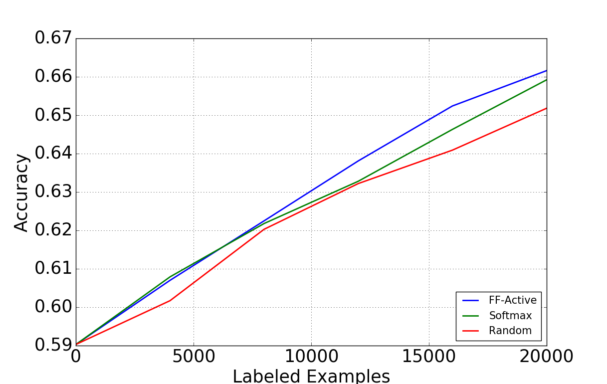
For CIFAR-100 we used an identical VGG-16 architecture to that used for CIFAR-10 (with the exception of the last output layer that now consisted of 100 units). We also used the same optimization algorithm and learning rate schedule. The construction of and was also identical to the CIFAR-10 experiment. The learning curves of FF-Active, SR, and Random are depicted in Figure 3. Here again we see a consistent advantage of FF-Active over Random and near identical performance of FF-active and SR during the initial stage and then degradation of SR. While the relative advantage of FF-Active over Random appears to be smaller in CIFAR-100 compared to CIFAR-10, the overall accuracy slope (accuracy improvement vs. labeled examples) is larger in CIFAR-100 than in CIFAR-10. Also, we observe that the gap between FF-Active and Random is increasing (in both CIFAR-100 and CIFAR-10). It would, therefore, be very interesting to examine what the result would be using a very large pool (a really long tail); hence, our next experiment.
4.4 The Longer Tail – Synthetically Inflated Pool
Our active learning setting is designed to model potential label complexity saving over a prolonged active session where more and more examples are available for labeling. While we expect this scenario to occur in future applications of machine learning models, currently available datasets aren’t large enough to model this scenario.
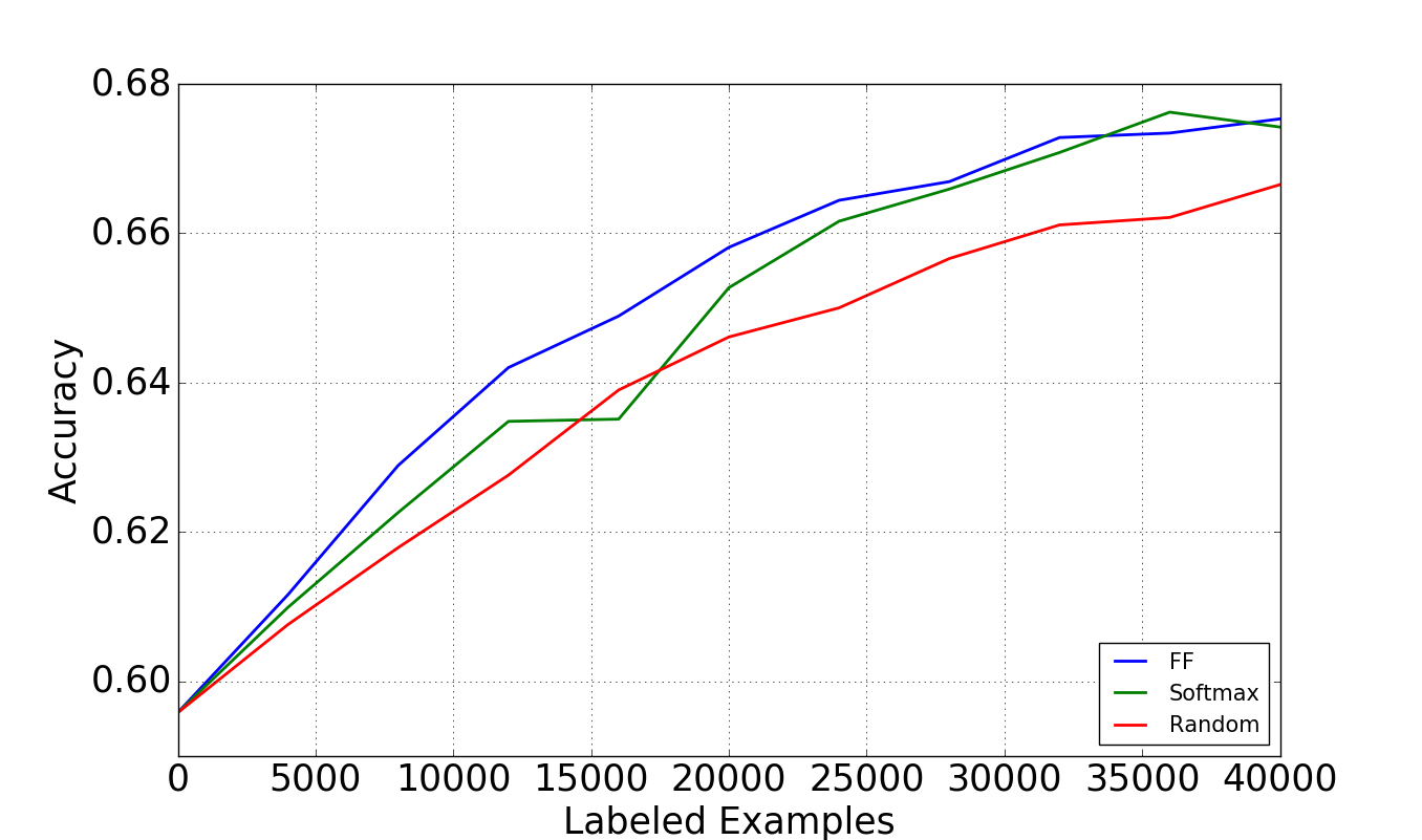
For the experiments in this section, we synthetically created a larger dataset, based on a CIFAR-100, attempting to model a larger pool. Specifically, we inflated the CIFAR-100 pool by a factor of three, using bootstrap sampling (sampling with replacement). We experimented with the resulting inflated CIFAR-100 using the same experimental setting described in Section 4.3. The unlabeled pool in this experiment contains 150,000 images. Here we observe a very significant domination of FF-Active over Random, and domination of FF-Active over SR through most of the session.
5 Inspecting of FF and SR over a Small Synthetic Example
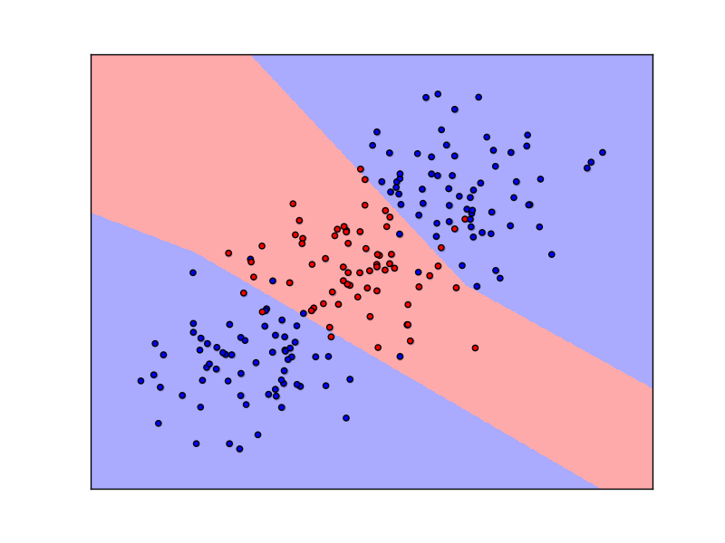
In this section we observe more closely the behavior of the querying functions of FF-Active and SR, and demonstrate that their strategies are quite different. The FF-Active strategy conducts systematic exploration in the sense that its next query is always on the point least represented by the current coreset (using the metric we choose to employ in the underlying representation space). On the other hand, SR is focused on exploiting (refining) the region around the decision boundary. We demonstrate this difference by simulating the methods over a synthetic dataset representing the binary learning problem depicted in Figure 5(a). In this figure there are 200 points randomly sampled from three Gaussians in . The middle Gaussian represents the negative class (red) and the two other Gaussians represents the positive class (blue). Assume that we randomly received two labeled points, one in each class, to initialize an active learning session for both FF-Active and SR. All other points at this stage consist the unlabeled pool (depicted in faded green). A neural network with one hidden layer is in use, in Figure 5(b) where the initial classifier is depicted together with the two initial labeled points. We now independently apply the two algorithms (FF-Active and SR) starting from this initial state. At each round we compute the next query, receive its label, and revise the decision boundary by re-training the model with the revised training set. Figure 5 depicts the results of the two simulations. It is evident that FF-Active effectively captures the geometry of the problem using much fewer queries than SR.
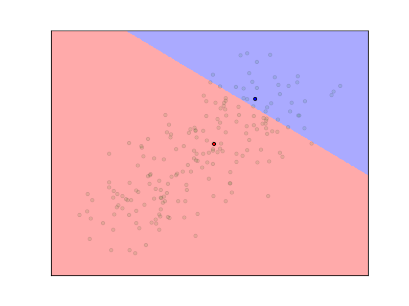
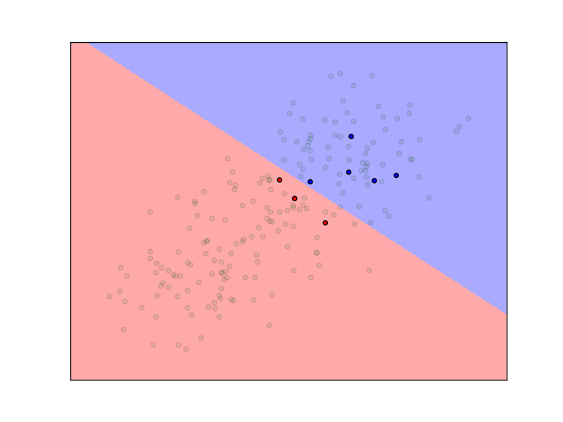
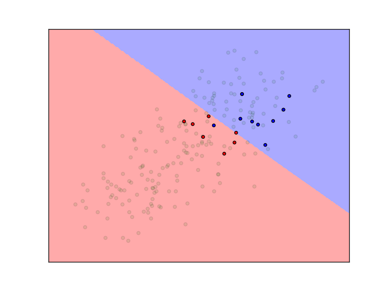
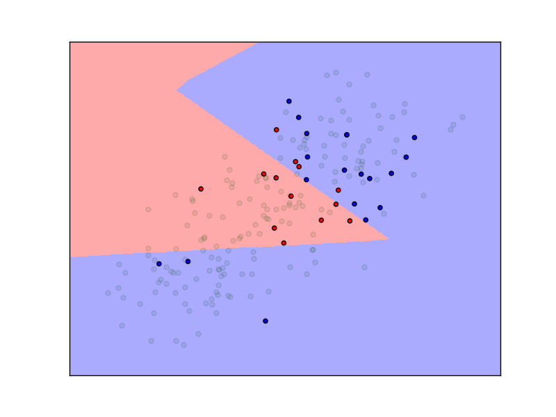
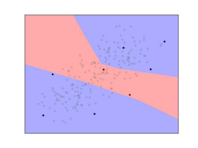
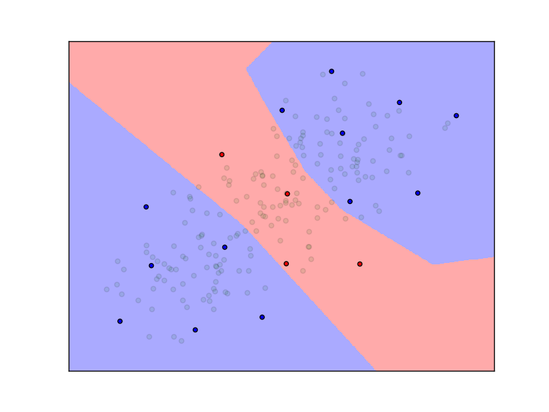
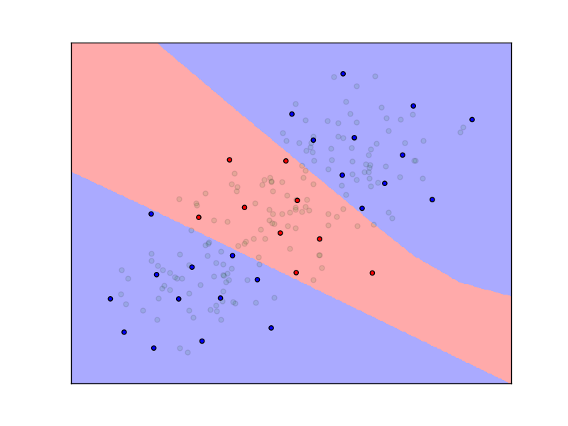
This simulation nicely illustrates the conceptual difference between the two strategies. Whereas FF-Active was able to almost perfectly identify the best model with 6 queries, SR is still far away with 30 queries. The caveat here is that this simulation is focused on an early stage of the active learning process, and we are interested in the later stages (the “long tail”). We speculate that in complex problems such as CIFAR-10 and CIFAR-100 (noisy, high dimensional, and multi-class), extensive exploration is required throughout the game over the representation space created by the DNN. We leave this interesting question for future research.
6 Concluding Remarks
Previous studies indicate that without prior knowledge or hindsight, active learning cannot be be effectively performed. In this paper we focus on a setting where an initial reasonable model has already been trained and only then we start to learn actively. Our results indicate that considerable labeling resources can be saved using an active algorithm whose goal is to improve this initial model.
Motivated by compression ideas, our main contribution is a novel pool-based active learning algorithm for deep nets achieving clear and significant advantage over passive learning. The traditional softmax-response (SR) technique that has been previously considered for deep active learning is also useful in this setting, but is inferior to our method. Overall, we believe that the proposed method provides a viable and practical tool that will work ‘out-of-the-box’ on image data and possibly on other types of data.
The main idea behind our new querying function is the use of model-based coresets for compressing the input data based on its internal representation over the space defined by neuronal activations over a representation layer. The specific coreset engine in our case is the greedy farthest-first traversal. Many other interesting and perhaps more powerful coreset engines can be considered, such as large margin coresets (Har-Peled et al., 2007), coresets used for DP-means clustering (Bachem et al., 2015), and coresets developed for dimensionality reduction (Feldman et al., 2016), to name a few. Of course, by adapting the coreset view, it would be very interesting to prove approximation guarantees for neural networks using existing or new techniques.
Other improvements of the proposed method would be very interesting to consider. For example, the use pseudo-labeling can allow for stratified coresets, and also enable inferring true labels using high confidence principles (Geifman & El-Yaniv, 2017). We also believe that using the Monte-Carlo dropout technique of Gal et al. (2017), we can effectively generate an ensemble of representations and reduce the variance in our traversal predictions, possibly decreasing the label complexity.
Finally, we would like to emphasize the open question whose study motivated this work. Would it be possible to compress datasets such as CIFAR-100 or Imagenet to a (logarithmic) fraction of their size while maintaining high classification performance? Any significant advancement in this direction is likely to substantially advance deep active learning and moreover, can potentially establish a theoretical breakthrough in the theory of deep learning using compression scheme techniques of statistical learning theory (David et al., 2016).
Acknowledgments
This research was supported by The Israel Science Foundation (grant No. 1890/14)
References
- Bachem et al. (2015) Olivier Bachem, Mario Lucic, and Andreas Krause. Coresets for nonparametric estimation-the case of dp-means. In International Conference on Machine Learning, pp. 209–217, 2015.
- Balcan & Long (2013) Maria-Florina Balcan and Phil Long. Active and passive learning of linear separators under log-concave distributions. In Conference on Learning Theory, pp. 288–316, 2013.
- Balcan et al. (2006) M.F. Balcan, A. Beygelzimer, and J. Langford. Agnostic active learning. In Proceedings of the 23rd international conference on Machine learning, pp. 65–72. ACM, 2006.
- Baram et al. (2004) Yoram Baram, Ran El Yaniv, and Kobi Luz. Online choice of active learning algorithms. Journal of Machine Learning Research, 5(Mar):255–291, 2004.
- Cohn et al. (1994) D. Cohn, L. Atlas, and R. Ladner. Improving generalization with active learning. Machine Learning, 15(2):201–221, 1994.
- David et al. (2016) Ofir David, Shay Moran, and Amir Yehudayoff. Supervised learning through the lens of compression. In D. D. Lee, M. Sugiyama, U. V. Luxburg, I. Guyon, and R. Garnett (eds.), Advances in Neural Information Processing Systems 29, pp. 2784–2792. Curran Associates, Inc., 2016.
- El-Yaniv & Wiener (2012) R. El-Yaniv and Y. Wiener. Active learning via perfect selective classification. Journal of Machine Learning Research, 13:255–279, 2012.
- Feldman et al. (2016) Dan Feldman, Mikhail Volkov, and Daniela Rus. Dimensionality reduction of massive sparse datasets using coresets. In Advances in Neural Information Processing Systems, pp. 2766–2774, 2016.
- Freund et al. (1993) Y. Freund, H.S. Seung, E. Shamir, and N. Tishby. Information, prediction, and Query by Committee. In Advances in Neural Information Processing Systems (NIPS) 5, pp. 483–490, 1993.
- Gal et al. (2017) Yarin Gal, Riashat Islam, and Zoubin Ghahramani. Deep bayesian active learning with image data. arXiv preprint arXiv:1703.02910, 2017.
- Geifman & El-Yaniv (2017) Yonatan Geifman and Ran El-Yaniv. Selective classification for deep neural networks. In Advances in neural information processing systems, 2017.
- Gonzalez (1985) Teofilo F Gonzalez. Clustering to minimize the maximum intercluster distance. Theoretical Computer Science, 38:293–306, 1985.
- Hanneke (2013) S. Hanneke. A statistical theory of active learning. Unpublished, 2013.
- Har-Peled et al. (2007) Sariel Har-Peled, Dan Roth, and Dav Zimak. Maximum margin coresets for active and noise tolerant learning. In IJCAI, pp. 836–841, 2007.
- Hochbaum (1996) Dorit S Hochbaum. Approximation algorithms for NP-hard problems. PWS Publishing Co., 1996.
- Huang et al. (2015) Tzu-Kuo Huang, Alekh Agarwal, Daniel J Hsu, John Langford, and Robert E Schapire. Efficient and parsimonious agnostic active learning. In Advances in Neural Information Processing Systems, pp. 2755–2763, 2015.
- Krizhevsky & Hinton (2009) Alex Krizhevsky and Geoffrey Hinton. Learning multiple layers of features from tiny images. 2009.
- LeCun et al. (1998) Yann LeCun, Léon Bottou, Yoshua Bengio, and Patrick Haffner. Gradient-based learning applied to document recognition. Proceedings of the IEEE, 86(11):2278–2324, 1998.
- Phillips (2016) Jeff M Phillips. Coresets and sketches. arXiv preprint arXiv:1601.00617, 2016.
- Simonyan & Zisserman (2014) Karen Simonyan and Andrew Zisserman. Very deep convolutional networks for large-scale image recognition. arXiv preprint arXiv:1409.1556, 2014.
- Tong & Koller (2001) Simon Tong and Daphne Koller. Support vector machine active learning with applications to text classification. Journal of machine learning research, 2(Nov):45–66, 2001.
- Wang et al. (2016) Keze Wang, Dongyu Zhang, Ya Li, Ruimao Zhang, and Liang Lin. Cost-effective active learning for deep image classification. IEEE Transactions on Circuits and Systems for Video Technology, 2016.
- Zhou et al. (2013) Shusen Zhou, Qingcai Chen, and Xiaolong Wang. Active deep learning method for semi-supervised sentiment classification. Neurocomputing, 120:536–546, 2013.
