Quotients of graph operators by symmetry representations

Abstract.

A finite dimensional operator that commutes with some symmetry group admits quotient operators, which are determined by the choice of associated representation. Taking the quotient isolates the part of the spectrum supporting the chosen representation and reduces the complexity of the spectral problem. Yet, such a quotient operator is not uniquely defined. Here we present a computationally simple way of choosing a special basis for the space of intertwiners, allowing us to construct a quotient that reflects the structure of the original operator. This quotient construction generalizes previous definitions for discrete graphs, which either dealt with restricted group actions or only with the trivial representation.

We also extend the method to quantum graphs, which simplifies previous constructions within this context, answers an open question regarding self-adjointness and offers alternative viewpoints in terms of a scattering approach. Applications to isospectrality are discussed, together with numerous examples and comparisons with previous results.

1. Introduction

The analysis of linear operators possessing a certain symmetry dates backs to the seminal works of Schur and Weyl [Sch27, Wey46]. More specifically, given a linear representation $\pi$ of a group $G$, they studied the properties of the algebra of matrices $M$ satisfying $\pi(g)M=M\pi(g)$ for all $g\in G$. Their answer — that by a suitable change of basis $M$ can be decomposed into blocks associated with the irreducible representations of $\pi$ — is a cornerstone of modern representation theory.

For a given particular system, a quantum Hamiltonian for example, representation theory is often used to classify the states and thus deduce the properties of the full system. In order to isolate the states of a particular representation one must ‘desymmetrize’ in some appropriate manner, or, equivalently, find the corresponding block of the reduced linear operator. This philosophy underlies, for instance, the Floquet–Bloch–Gelfand transform of periodic operators [RS78, Sec. XIII.16], [Kuc16], where the symmetry group $\mathbb{Z}^{d}$ is abelian and thus has particularly simple irreducible representations. With regards to discrete symmetries, this philosophy has been utilized, for example, to construct trace formulae [Rob89, Lau91] and analyze the spectral statistics [KR97, JMS12] of quantum chaotic systems with symmetries. A more systematic construction procedure applicable to unbounded self-adjoint operators on metric graphs and manifolds was demonstrated by Band, Parzanchevski and Ben-Shach [BPBS09, PB10], who showed how one may perform this desymmetrization for arbitrary representations of a discrete group of symmetries. The resulting desymmetrized system was termed a ‘quotient graph’ or ‘quotient manifold’. In particular, this notion generalized Sunada’s method [Sun85] for constructing pairs of isospectral manifolds, famously used by Gordon, Webb and Wolpert [GWW92a, GWW92b] to answer negatively Marc Kac’s question ‘Can one hear the shape of a drum?’ [Kac66]. Joyner, Müller and Sieber [JMS14] utilized the quotient graph technique to propose a spin-less quantum system whose spectrum exhibits the Gaussian symplectic ensemble statistics from random matrix theory; this effect was later demonstrated experimentally [RAJ⁺16]. The quotient construction has also been used to prove the existence of conical points in the dispersion relation of graphene by Berkolaiko and Comech [BC18].

The main result of this work is a compact and transparent formula (Definition 2.2) that extracts the ‘quotient of an operator by a representation of its symmetry group’, or quotient operator for short, in the context of finite dimensional operators. While the topic is a classical one, the formula appears to be new; it generalizes previous works by Brooks [Bro99a, Bro99b], Chung and Sternberg [CS92], and Halbeisen and Hungerbühler [HH99] that either dealt with restricted group actions or only with the trivial representation.

We chose to state our main result, equation (2.5), as a definition and then prove, in Sections 2.2-2.4, that it has the properties one expects from a desymmetrized part of an operator that corresponds to a particular representation. While formulated for general matrices, our results are geared towards spectral analysis of graphs in that the connectivity structure of the original operator is reflected in the quotient operator. Naturally, this is the effect of a particular choice of basis we make.

To illustrate the types of results one obtains by using the quotient construction, we present some examples.

Example 1.1.

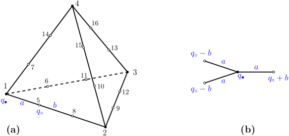
Figure 1.1. (a) A graph with symmetry group $S_{4}$ acting as permutations of the vertices $1,2,3,4$ and the corresponding permutation of other vertices. The graph is associated with the operator T in (1.1).
(b) A graph which is associated to the quotient operator $\textrm{T}_{\sigma}$ given by (1.3). This quotient operator captures all the T eigenvalues of multiplicity three.

Consider the graph on 16 vertices shown in Figure 1.1(a) and a corresponding family of operators $\textrm{T}:\mathbb{C}^{16}\to\mathbb{C}^{16}$ that are invariant under the action of the symmetry group $G=S_{4}$ induced by permuting the vertices $1$, $2$, $3$ and $4$. Explicitly, grouping the vertices into two sets, $O_{\bullet}=\{1,\ldots,4$} and $O_{\circ}=\{5,\ldots,16\}$, we let

$$\textrm{T}_{ij}=\begin{cases}a&\mbox{if }i\sim j,\ \ i\in O_{\bullet},j\in O_{\circ}\mbox{ or }i\in O_{\circ},j\in O_{\bullet}\\ b&\mbox{if }i\sim j,\ \ i\in O_{\circ},j\in O_{\circ}\\ q_{\bullet}&\mbox{if }i=j\in O_{\bullet}\\ q_{\circ}&\mbox{if }i=j\in O_{\circ},\end{cases}$$ (1.1)

where $\sim$ indicates adjacency of the vertices.

For every choice of the parameters $a,b,q_{\bullet},q_{\circ}\in\mathbb{C}$, there are at least four triply degenerate eigenvalues in the spectrum of T (typically, all other eigenvalues have lower multiplicity). To give a numerical example, the choice $a=b=-1$, $q_{\bullet}=3$, $q_{\circ}=2$ in (1.1) yields the spectrum

$$\mathrm{Spec}(\textrm{T})=\{0,\ \mathbf{0.44},\ \mathbf{0.44},\ \mathbf{0.44},\ 1,\ 1,\ \mathbf{2},\ \mathbf{2},\ \mathbf{2},\ \mathbf{3},\ \mathbf{3},\ \mathbf{3},\ 4,\ \mathbf{4.56},\ \mathbf{4.56},\ \mathbf{4.56}\}.$$ (1.2)

It is well known that the eigenvalue multiplicities arise due to the symmetry of the operator. More precisely, they can be traced to the 3-dimensional irreducible representations of the group $S_{4}$ by studying the action of T on the space of intertwiners. The current work offers a simple prescription for extracting these eigenvalues in the form of the spectrum of a smaller graph, shown in this particular case in Figure 1.1(b) and given explicitly by

$$\textrm{T}_{\sigma}=\begin{pmatrix}q_{\bullet}&a&a&a\\ a&q_{\circ}-b&0&0\\ a&0&q_{\circ}-b&0\\ a&0&0&q_{\circ}+b\end{pmatrix}.$$ (1.3)

To compare to (1.2), substituting $a=b=-1$, $q_{\bullet}=3$, $q_{\circ}=2$, we get

$$\mathrm{Spec}(\textrm{T}_{\sigma})=\{0.44,\ 2,\ 3,\ 4.56\}.$$ (1.4)

The details of the derivation of (1.3) are contained in Example 3.3 and 4.11.

While the main body of the paper deals with finite-dimensional operators, in Section 4 we show how to use it to compute quotients of unbounded self-adjoint operators on metric (“quantum”) graphs, where one has to be careful to take an appropriate quotient of the operator’s domain. Thus we are simplifying and making more explicit the constuction of [BPBS09, PB10], incidentally proving that it preserves self-adjointness. Delaying all details to Section 4, we present here an example of a non-trivial quotient.

Example 1.2.

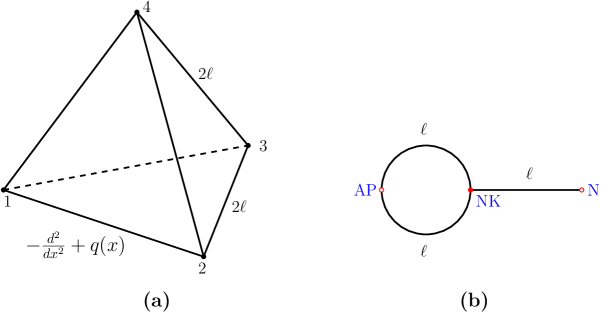
Figure 1.2. A quantum graph with symmetry group $S_{4}$ and its quotient that captures the eigenvalues of multiplicity three.

Consider a quantum graph analogue of Example 1.1, namely the graph in Fig. 1.2(a). We defer the rigorous description of the corresponding differential operator $\Gamma$ to Section 4; here we just mention that all edges have the same length $2\ell$, all vertices have Neumann-Kirchhoff (NK or “standard”) conditions and the potential is assumed to be symmetric with respect to reflection around the midpoint, $q(2\ell-x)=q(x)$.

The symmetry group here is $S_{4}$, so the presence of eigenvalues of multiplicity three is not surprising. What is remarkable is that those eigenvalues are exactly the eigenvalues of the graph shown in Fig. 1.2(b), where the central vertex has NK conditions, right vertex has Neumann and the left vertex has anti-periodic conditions. As above, the main result of this work is representing the action of the original graph operator on an appropriate invariant subspace as a concrete operator on a smaller graph.

The paper is structured as follows. Our main results are presented in Section 2, where we define the quotient by a compact formula in Definition 2.2 and then, in Theorem 2.5 and Propositions 2.6 and 2.8, establish its various algebraic and spectral properties. Section 3 provides several examples that illustrate the group-theoretic constructions used in the proofs of Section 2. In Section 4 we adapt the quotient operator construction (back) to quantum graphs and show how this broadens the previous results in [BPBS09, PB10]. Section 5 outlines some further applications of the current results and explains how they extend previous works on isospectrality [Bro99a, Bro99b, HH99] and eigenvalue computation [CDS95, CS92, Chu97].

At the end, Appendix A contains the necessary background material on representation theory, in particular on Frobenius isomorphism. Due to our motivation coming from self-adjoint operators, our emphasis is on the preservation of the Hilbert structure, which is not usually covered in algebra-themed textbooks. Appendix B contains the proofs of the results from Section 4.

2. Quotient Operators - definitions and main properties

This paper (and in particular the current section) is substantially based on elements from representation theory. For completness, we describe the relevant definitions and statements in Appendix A.

2.1. Defining the quotient operator

This subsection defines the main object of this paper — the quotient operator. Examples illustrating the construction of the quotient operator and its properties are collected in Section 3. A reader less familiar with the topic is encouraged to consult these examples while reading this section.

Definition 2.1 (symmetric operator).

Let $G$ be a finite group and $\textrm{V}_{\pi}$ be a vector space over $\mathbb{C}$ which is a $G$-module. We say that a linear operator $\textrm{T}:\textrm{V}_{\pi}\to\textrm{V}_{\pi}$ is $G$-symmetric (or that T commutes with $G$) if

$$\forall\ g\in G,\quad g\,\textrm{T}=\textrm{T}\,g.$$ (2.1)

That $\textrm{V}_{\pi}$ is a $G$-module means that the group $G$ acts on $\textrm{V}_{\pi}$ by linear transformations, i.e. it is a representation of $G$. In the following, it will be convenient to use the terminology of $G$-modules and group representations, interchangeably. The reader is referred to Appendix A for the corresponding background and for further details.

We will use the symmetry of the operator T to construct a new operator, which we call the quotient operator. We will restrict ourselves to the case when the $G$-module $\textrm{V}_{\pi}$ is finite dimensional and corresponds to some permutation representation $\pi:G\rightarrow GL(\textrm{V}_{\pi})$. Namely, we assume that all $g\in G$ act as permutation matrices, for a suitably chosen basis of $\textrm{V}_{\pi}$. We will refer to this basis as the standard basis, $\{\mathbf{e}_{i}\}_{i\in\mathcal{P}}$, where the corresponding index set is $\mathcal{P}:=\{1,\ldots,p\}$, with $p:=\dim\textrm{V}_{\pi}$. Hence, $\textrm{V}_{\pi}\cong\mathbb{C}[\mathcal{P}]$. In what follows, we use both $\textrm{V}_{\pi}$ and $\mathbb{C}[\mathcal{P}]$ interchangeably, depending on whether we wish to emphasize that it is a $G$-module, or rather that these are functions on the point set $\mathcal{P}$.

The permutation action of $G$ on the standard basis $\{\mathbf{e}_{i}\}$ induces an action of $G$ on the index set $\mathcal{P}$, namely $g\thinspace\mathbf{e}_{i}=\mathbf{e}_{g\thinspace i}$. We use this action to decompose $\mathcal{P}$ into orbits,

$$O_{i}:=\{j\in\mathcal{P}~{}:~{}j=g\thinspace i~{}\textrm{for some }g\in G\},$$ (2.2)

and choose a representative of each orbit. Without loss of generality, we denote those representatives by $\mathcal{D}=\{1,\ldots,\left|\mathcal{D}\right|\}$ and call $\mathcal{D}$ a fundamental domain.

Let $\textrm{V}_{\rho}$ be another finite-dimensional $G$-module and denote $r:=\dim\textrm{V}_{\rho}$. We assume that $\textrm{V}_{\rho}$ is equipped with an inner product (hence, it is a Hilbert space) and that the $G$ action preserves this inner product (equivalently, that the representation $\rho$ is unitary).

We start connecting $\textrm{V}_{\rho}$ with $\textrm{V}_{\pi}$, towards defining the quotient operator (of T with respect to $\textrm{V}_{\rho}$). For each index $i\in\mathcal{D}$ consider the stabilizer group

$$G_{i}:=\{g\in G:g\thinspace i=i\},$$ (2.3)

and define the $G_{i}$-invariant subspace of $\textrm{V}_{\rho}$ by

$$(\textrm{V}_{\rho})^{G_{i}}:=\left\{v\in\textrm{V}_{\rho}~{}:~{}\forall g\in G_{i},~{}gv=v\right\},$$ (2.4)

For each $i\in\mathcal{D}$, denote $d_{i}:=\dim(\textrm{V}_{\rho})^{G_{i}}$ and pick $\{\varphi_{i}^{(n)}\}_{n=1}^{d_{i}}$ to be an orthonormal basis for $(\textrm{V}_{\rho})^{G_{i}}$, with respect to the inner product inherited from $\textrm{V}_{\rho}$. For use in the next definition, we collect all vectors $\{\varphi_{i}^{(n)}\}_{n=1}^{d_{i}}$ as the columns of a matrix, which we denote by $\Phi_{i}$. Namely, $\Phi_{i}$ is an $r\times d_{i}$ matrix providing an isometry between $\mathbb{C}^{d_{i}}$ and $(\textrm{V}_{\rho})^{G_{i}}$. We further denote $d:=\sum_{i\in\mathcal{D}}d_{i}$.

Definition 2.2 (Quotient operator).

Using the notation introduced above, we define $\textrm{T}_{\rho}$ to be a $d\times d$ matrix, which is comprised of $\left|\mathcal{D}\right|\times\left|\mathcal{D}\right|$ blocks. The $(i,j)$-th block is is the following $d_{i}\times d_{j}$ matrix

$$\left[\textrm{T}_{\rho}\right]_{i,j} :=\frac{1}{\sqrt{|G_{i}||G_{j}|}}\Phi_{i}^{*}\,\left(\sum_{g\in G}\textrm{T}_{i,gj}\,g\right)\,\Phi_{j}.$$ (2.5)

$\textrm{T}_{\rho}$ is called the quotient operator of T with respect to $\textrm{V}_{\rho}$.

Remark 2.3.

The notation of quotient operator includes only the auxiliary $G$-module, $\textrm{V}_{\rho}$, with respect to which the quotient is constructed. The $G$-module $\textrm{V}_{\pi}$ is understood from the context, as it is the domain of the original operator, $T$. The term “quotient operator” arises from the specific case when $\textrm{V}_{\rho}$ is the trivial representation of $G$ (see Corollary 2.4). In this case the domain of $\textrm{T}_{\rho}$ is the quotient $\nicefrac{{\textrm{V}_{\pi}}}{{G}}$ (in the topological sense). Hence, we adopt the name quotient also for the more general case (as was already done in the previous works [BPBS09, PB10]).

Before presenting the properties of the quotient operator, we mention a few general cases in which formula (2.5) reduces to a simpler form. These are useful in various applications, some of which are surveyed in Section 5. In particular, when T is a discrete graph operator, the special case of the quotient with respect to the trivial representation, (2.6), is a well-known concept. It is known by various names such as a graph divisor, an equitable partition, a coloration, a quotient graph or an orbigraph (more details on these special cases are given in Section 5.2).

Corollary 2.4 (Simplifications and variations of the formula).

1. Trivial representation: If $\textrm{V}_{\rho}$ is the trivial $G$-module then $\textrm{T}_{\rho}$ is a $\left|\mathcal{D}\right|\times\left|\mathcal{D}\right|$ matrix whose entries are

   $$[\textrm{T}_{\rho}]_{i,j}=\frac{1}{\sqrt{|G_{i}||G_{j}|}}\sum_{g\in G}\textrm{T}_{i,gj}.$$ (2.6)

2. Free action: If the action of $G$ on $\mathcal{P}$ is free then for all $i,j\in\mathcal{D}$, the $(i,j)$-th block of $\textrm{T}_{\rho}$ is given by

   $$[\textrm{T}_{\rho}]_{i,j}=\sum_{g\in G}\textrm{T}_{i,gj}\,g.$$ (2.7)

3. Double coset expansion: $\left[\textrm{T}_{\rho}\right]_{i,j}$ can also be computed as

   $$\left[\textrm{T}_{\rho}\right]_{i,j}=\sqrt{\left|G_{i}\right|\left|G_{j}\right|}\Phi_{i}^{*}\left(\sum_{G_{i}gG_{j}\in G_{i}\backslash G/G_{j}}\frac{1}{\left|G_{i}g\cap gG_{j}\right|}\textrm{T}_{i,gj}\,g\right)\Phi_{j},$$ (2.8)

   where the sum is over representatives of the double cosets $G_{i}\backslash G/G_{j}$.

Proof of Corollary 2.4.

To get (2.6), note that $\Phi_{i}=(1)$ for all $i\in\mathcal{D}$. Substituting this into (2.5), we obatin that the $(i,j)$ block is just a single matrix entry given by (2.6).

To get (2.7) note that the free action, $G_{i}=\{1\}$, implies $(\textrm{V}_{\rho})^{G_{i}}\cong\textrm{V}_{\rho}$. Taking dimensions gives $d_{i}=r=\deg(\rho)$. Therefore, we can choose $\Phi_{i}$ to be any $r\times r$ unitary matrix, including $\Phi_{i}=\mathbb{\boldsymbol{I}}_{r}$. This yields (2.7).

To get (2.8) we only need to employ the decomposition of $G$ to doubles cosets $G_{i}\backslash G/G_{j}$ and note that the expression $\left(\Phi_{i}^{*}\,\left[\textrm{T}\right]_{i,gj}\rho(g)\,\Phi_{j}\right)$ is invariant with respect to the choice of particular representative of the double coset and that $\left|G_{i}gG_{j}\right|=\frac{\left|G_{i}\right|\left|G_{j}\right|}{\left|G_{i}g\cap gG_{j}\right|}$. Hence, in (2.5) we may only sum over representatives of the double cosets $G_{i}\backslash G/G_{j}$ to get (2.8). ∎

2.2. Fundamental property of the quotient operator

We present here a fundamental property which the quotient operator defined by equation (2.5) satisfies and from which follow other algebraic and spectral properties of the quotient. To do so, we need to introduce a few more algebraic notions. Let $G$ be a finite group and $\textrm{V}_{\rho}$ and $\textrm{V}_{\pi}$ be two finite-dimensional $G$-modules. As before we assume that $\textrm{V}_{\rho}$ and $\textrm{V}_{\pi}$ are, equipped with inner products, which are preserved by the $G$ action. We consider all linear maps from $\textrm{V}_{\rho}$ to $\textrm{V}_{\pi}$ which commute with the group action, and denote this set by

$$\mathrm{Hom}_{G}(\textrm{V}_{\rho},\textrm{V}_{\pi}):=\left\{\phi\in\mathrm{Hom}(\textrm{V}_{\rho},\textrm{V}_{\pi})~{}:~{}g\phi=\phi g\right\}.$$ (2.9)

This is a vector space whose elements are commonly called intertwiners (see more in Appendix A). The natural inner product on $\mathrm{Hom}_{G}$ is the Frobenius product

$$\left<\phi_{1},\phi_{2}\right>_{\mathrm{Hom}_{G}(\textrm{V}_{\rho},\textrm{V}_{\pi})}:=\textrm{Tr}\left(\phi_{2}^{*}\phi_{1}\right)=\sum_{v\in B(\textrm{V}_{\rho})}\left<\phi_{1}(v),\phi_{2}(v)\right>_{\textrm{V}_{\pi}},$$ (2.10)

where $\left<\cdot,\cdot\right>_{\textrm{V}_{\pi}}$ denotes the inner product in $\textrm{V}_{\pi}$ and $B(\textrm{V}_{\rho})$ is a basis for $\textrm{V}_{\rho}$. Let $\textrm{T}:\textrm{V}_{\pi}\rightarrow\textrm{V}_{\pi}$ be a linear operator which is $G$-symmetric. Such an operator acts on each intertwiner $\phi\in\mathrm{Hom}_{G}(\textrm{V}_{\rho},\textrm{V}_{\pi})$ by composition,

$$\forall u\in\textrm{V}_{\rho},\quad\quad\left(\textrm{T}\phi\right)(u):=\textrm{T}\thinspace\phi(u).$$ (2.11)

Clearly, $\textrm{T}\phi\in\mathrm{Hom}(\textrm{V}_{\rho},\textrm{V}_{\pi})$. But we even have $\textrm{T}\phi\in\mathrm{Hom}_{G}(\textrm{V}_{\rho},\textrm{V}_{\pi})$ since

$$g(\textrm{T}\phi)=\textrm{T}g\phi=(\textrm{T}\phi)g,$$ (2.12)

because T is $G$-symmetric and $\phi\in\mathrm{Hom}_{G}(\textrm{V}_{\rho},\textrm{V}_{\pi})$ commutes with $g$.

This linear action of T on $\mathrm{Hom}_{G}(\textrm{V}_{\rho},\textrm{V}_{\pi})$ leads to our main theorem.

Theorem 2.5 (Fundamental property of the quotient operator).

Let $G$ be a finite group and $\textrm{V}_{\rho},\textrm{V}_{\pi}$ two finite-dimensional $G$-modules, equipped with inner products, which are preserved by the group action. Let $\textrm{T}:\textrm{V}_{\pi}\rightarrow\textrm{V}_{\pi}$ be a linear operator which is $G$-symmetric.

Then the quotient operator of T with respect to $\textrm{V}_{\rho}$ is unitarily equivalent to $\left.\textrm{T}\right|_{\mathrm{Hom}_{G}(\textrm{V}_{\rho},\textrm{V}_{\pi})},$

$$\textrm{T}_{\rho}\cong\left.\textrm{T}\right|_{\mathrm{Hom}_{G}(\textrm{V}_{\rho},\textrm{V}_{\pi})}.$$ (2.13)

Namely, there exists an ortonormal basis of $\mathrm{Hom}_{G}(\textrm{V}_{\rho},\textrm{V}_{\pi})$ with respect to which the matrix form of $\left.\textrm{T}\right|_{\mathrm{Hom}_{G}(\textrm{V}_{\rho},\textrm{V}_{\pi})}$ is $\textrm{T}_{\rho}$.

We postpone the proof of the theorem to the end of Section 2 and first present the various properties which follow from the theorem.

2.3. Algebraic and spectral properties of the quotient

We start by summarizing some of the algebraic properties of the quotient operator. These are general properties arising from basic representation theory, and have useful applications. In particular, Proposition  2.6 (3) is a vital component in the construction of isospectral objects [BPBS09, PB10] (see Section 5.1) and Proposition 2.6 (2) is the well-known decomposition of a symmetric operator, following from Schur’s Lemma (see Section 5.2 and [CDS95, sec. 5]).

Recall that we assume $G$ is a finite group and that the $G$-modules $\textrm{V}_{\pi}$ and $\textrm{V}_{\rho}$ are finite-dimensional and with inner products preserved by the group action. We denote $\mathrm{V}_{\rho_{1}}\cong\mathrm{V}_{\rho_{2}}$ when the $G$-modules $\mathrm{V}_{\rho_{1}}$ and $\mathrm{V}_{\rho_{2}}$ are isomorphic as Hilbert spaces (i.e., unitarily isomorphic) and this isomorphism commutes with the $G$-action. We use a similar notation $\textrm{T}_{1}\cong\textrm{T}_{2}$ to denote that the operators $\textrm{T}_{1}$ and $\textrm{T}_{2}$ are unitarily equivalent.

Proposition 2.6.

[Algebraic properties]

Let $G$ be a finite group. Let T be a $G$-symmetric linear operator.

1. Let $\mathrm{V}_{R}\cong\bigoplus_{\rho}\textrm{V}_{\rho}$ be a $G$-module which is isomorphic to the (orthogonal) direct sum of some (possibly repeating and not necessarily irreducible) $G$-modules $\textrm{V}_{\rho}$, then

   $$\textrm{T}_{R}\cong\bigoplus_{\rho}\textrm{T}_{\rho}.$$ (2.14)

2. Let $\textrm{reg}_{G}$ denote the regular representation of $G$. Then

   $$\textrm{T}\cong\textrm{T}_{\textrm{reg}_{G}}\cong\bigoplus_{\rho}\left[\mathbb{\boldsymbol{I}}_{\deg\rho}\otimes\textrm{T}_{\rho}\right],$$ (2.15)

   where the direct sum above is over all irreducible representations $\rho$ of $G$, and $\mathbb{\boldsymbol{I}}_{\deg\rho}$ is the identity operator of rank $\deg\rho$.
   

3. Let $H$ be a subgroup of $G$. If $\textrm{V}_{\sigma}$ is an $H$-module and $\textrm{V}_{\rho}=\textrm{$\mathrm{Ind}$}_{H}^{G}\left(\textrm{V}_{\sigma}\right)$ is the corresponding induced $G$-module from $H$ to $G$, then

   $$\textrm{T}_{\sigma}\cong\textrm{T}_{\rho}.$$ (2.16)

Remark 2.7.

Appendix A contains a short introduction on induced modules and representations.

Proof.

To prove (2.14), we note that $\mathrm{Hom}_{G}(\mathrm{V}_{R},\textrm{V}_{\pi})$ is isomorphic to $\bigoplus_{\rho}\mathrm{Hom}_{G}(\textrm{V}_{\rho},\textrm{V}_{\pi})$ as vector spaces (see, e.g. [DF04, ch. 10]). In addition, it is not hard to verify that this isomorphism preserves the inner product. Hence, (2.14) follows straightforwardly from the orthogonal decomposition $\mathrm{Hom}_{G}(\mathrm{V}_{R},\textrm{V}_{\pi})\cong\bigoplus_{\rho}\mathrm{Hom}_{G}(\textrm{V}_{\rho},\textrm{V}_{\pi})$ together with Definition 2.5.

To prove (2.15), first note that the second equivalence follows from (2.14) together with the decomposition of the regular representation in terms of irreducible representations (see e.g., [Ser77, ch. 2.4]). To see that $\textrm{T}\cong\textrm{T}_{\textrm{reg}_{G}}$, we use that $\textrm{reg}_{G}=\textrm{$\mathrm{Ind}$}_{H}^{G}\left(\textrm{V}_{\sigma}\right)$, where $H=\{\mathrm{id}\}$ is the trivial subgroup of $G$ and $\textrm{V}_{\sigma}=\mathbb{C}$ is the trivial representation of $H$ (see Appendix A). We may now apply (2.16) and get that its right hand side is $\textrm{T}_{\textrm{reg}_{G}}$. It is left only to explain why the left hand side in (2.16) is just $\textrm{T}_{\sigma}=\textrm{T}$. To see this, it is enough to note that $\mathrm{Hom}_{H}(\textrm{V}_{\sigma},\textrm{V}_{\pi})\cong\mathrm{Hom}(\textrm{V}_{\sigma},\textrm{V}_{\pi})\cong\textrm{V}_{\pi}$, keeping in mind that $H=\{\mathrm{id}\}$ and $\textrm{V}_{\sigma}=\mathbb{C}$.

Finally, we prove (2.16). Frobenius reciprocity theorem (namely, Theorem A.4 (2) together with Proposition A.5) gives the Hilbert space isomorphism

$$\mathrm{Hom}_{H}(\textrm{V}_{\sigma},\textrm{V}_{\pi})\cong\mathrm{Hom}_{G}(\textrm{$\mathrm{Ind}$}_{H}^{G}\left(\textrm{V}_{\sigma}\right),\textrm{V}_{\pi})=\mathrm{Hom}_{H}(\textrm{V}_{\rho},\textrm{V}_{\pi}).$$ (2.17)

By Proposition A.7, this isomorphism commutes with $T$ and therefore establishes the unitary equivalence

$$T\big{|}_{\mathrm{Hom}_{H}(\textrm{V}_{\sigma},\textrm{V}_{\pi})}\simeq T\big{|}_{\mathrm{Hom}_{G}(\textrm{V}_{\rho},\textrm{V}_{\pi})}.$$ (2.18)

The conclusion follows from (2.13). ∎

In many instances, the main purpose for constructing the quotient operator $\textrm{T}_{\rho}$, is to isolate the spectral properties of T associated to a particular representation $\rho$. To state this formally, let us introduce the generalized $\lambda$-eigenspace of order $k$,

$$\mathbf{E}_{k}^{\textrm{T}}(\lambda):=\ker\left((\textrm{T}-\lambda)^{k}\right).$$ (2.19)

In particular $\mathbf{E}_{1}^{\textrm{T}}(\lambda)$ is the usual eigenspace corresponding to eigenvalue $\lambda$.

Proposition 2.8 (Spectral properties).

1. Let $\lambda\in\mathbb{C}$ and $k\in\mathbb{N}$. Then $\mathbf{E}_{k}^{\textrm{T}}(\lambda)$ is a $G$-module and

   $$\mathbf{E}_{k}^{\textrm{T}_{\rho}}(\lambda)\cong\mathrm{Hom}_{G}(\textrm{V}_{\rho},\mathbf{E}_{k}^{\textrm{T}}(\lambda)).$$ (2.20)

2. The eigenspace of $T$ is decomposed over the irreducible representations $\rho$ of $G$ as follows,

   $$\mathbf{E}_{k}^{\textrm{T}}(\lambda)\cong\bigoplus_{\rho}\textrm{V}_{\rho}\otimes\mathbf{E}_{k}^{\textrm{T}_{\rho}}(\lambda).$$ (2.21)

   In particular, denoting by $m^{\textrm{T}}(\lambda)$ either geometric or the algebraic multiplicity of $\lambda\in\mathbb{C}$ as an eigenvalue of T, we get

   $$m^{\textrm{T}}(\lambda)=\sum_{\rho}\deg\rho\cdot m^{\textrm{T}_{\rho}}(\lambda),$$ (2.22)

   where the sum above is over all irreducible representations $\rho$ of $G$.

3. If T is self-adjoint then $\textrm{T}_{\rho}$ is self-adjoint.

Proof.

For the first part of the proposition observe first that $\mathbf{E}_{k}^{\textrm{T}}(\lambda)\subset\textrm{V}_{\pi}$ already comes equipped with an action of $G$ and, furthermore, it is invariant under this action: for all $f\in\mathbf{E}_{k}^{\textrm{T}}(\lambda)$ and $g\in G$ we have

$$\left(\textrm{T}-\lambda\mathbb{\boldsymbol{I}}\right)^{k}\left(gf\right)=g\left(\textrm{T}-\lambda\mathbb{\boldsymbol{I}}\right)^{k}f=0.$$

Therefore, $\mathbf{E}_{k}^{\textrm{T}}(\lambda)$ is a $G$-module.

Further note that $\mathrm{Hom}_{G}(\textrm{V}_{\rho},\mathbf{E}_{k}^{\textrm{T}}(\lambda))$ is a subspace of $\mathrm{Hom}_{G}(\textrm{V}_{\rho},\textrm{V}_{\pi})$. Therefore, by (2.13),

$$\mathbf{E}_{k}^{\textrm{T}_{\rho}}(\lambda)\cong\mathbf{E}_{k}^{\textrm{T}|_{\mathrm{Hom}_{G}(\textrm{V}_{\rho},\textrm{V}_{\pi})}}(\lambda)=\left\{f\in\mathrm{Hom}_{G}(\textrm{V}_{\rho},\textrm{V}_{\pi})\colon(\textrm{T}-\lambda)^{k}f=0\right\}\\ =\left\{f\in\mathrm{Hom}_{G}(\textrm{V}_{\rho},\textrm{V}_{\pi})\colon f(v)\in\mathbf{E}_{k}^{\textrm{T}}(\lambda)\ \forall v\in\textrm{V}_{\rho}\right\}=\mathrm{Hom}_{G}(\textrm{V}_{\rho},\mathbf{E}_{k}^{\textrm{T}}(\lambda)).$$ (2.23)

The second part of the proposition is an immediate corollary of the unitary equivalence in (2.15).

For the third part of the proposition, it is enough to show that $\textrm{T}_{\rho}$ is symmetric (since all our spaces are finite-dimensional). Let $\phi_{1},\phi_{2}\in\mathrm{Hom}_{G}(\textrm{V}_{\rho},\textrm{V}_{\pi})$ and $B(\textrm{V}_{\rho})$ an orthonormal basis of $\textrm{V}_{\rho}$.

$$\left<\textrm{T}_{\rho}\phi_{1}\,,\,\phi_{2}\right>_{\mathrm{Hom}_{G}(\textrm{V}_{\rho},\textrm{V}_{\pi})} =\sum_{v\in B(\textrm{V}_{\rho})}\left\langle T\phi_{1}(v)\,,\,\phi_{2}(v)\right\rangle_{\textrm{V}_{\pi}}$$

$$=\sum_{v\in B(\textrm{V}_{\rho})}\left\langle\phi_{1}(v)\thinspace,\thinspace T\phi_{2}(v)\right\rangle_{\textrm{V}_{\pi}}=\left<\phi_{1}\,,\,\textrm{T}_{\rho}\phi_{2}\right>_{\mathrm{Hom}_{G}(\textrm{V}_{\rho},\textrm{V}_{\pi})},$$

where in the middle, we used that T is self-adjoint. Hence, $\textrm{T}_{\rho}$ is symmetric and self-adjoint. Proposition 2.8 provides an important application of the quotient construction. It is well known that each eigenspace corresponds to a representation of the symmetry group. Namely, that $\mathbf{E}_{k}^{\textrm{T}}(\lambda)$ is a $G$-module. A fundamental question is which representations (or $G$-modules) actually appear in T’s spectrum and in which frequency. Equivalently, we ask for which $G$-modules $\textrm{V}_{\rho}$, we have a nontrivial $\mathrm{Hom}_{G}(\textrm{V}_{\rho},\mathbf{E}_{k}^{\textrm{T}}(\lambda))$, and how frequently (in T’s spectrum) this happens. We are now able to answer this via formula (2.5) and equation (2.20). To find out whether a $G$-module $\textrm{V}_{\rho}$ appears in T’s spectrum, one first computes $\textrm{T}_{\rho}$ using (2.5). If the dimension of $\textrm{T}_{\rho}$ is non-zero then $\textrm{V}_{\rho}$ appears in T’s spectrum. The frequency of its appearance is given as the dimension ratio of $\textrm{T}_{\rho}$ and T. A similar analysis may be done for operators T which are not finite dimensional, such as the metric graph operators discussed in Section 4. The existence (or nonexistence) and frequency of various representations in the spectrum is nicely demonstrated in Example 3.3 for discrete graphs and in Examples 4.10, 4.11 for metric graphs. ∎

2.4. Proof of Theorem 2.5

Theorem 2.5 is proven with the aid of the following lemma, which describes the ortonormal basis with respect to which we may write $\left.\textrm{T}\right|_{\mathrm{Hom}_{G}(\textrm{V}_{\rho},\textrm{V}_{\pi})}$ to get $\textrm{T}_{\rho}$, as in the statement of Theorem 2.5.

Lemma 2.9.

For each $i\in\mathcal{D}$ and $1\leq n\leq d_{i}$, let $\theta_{i}^{(n)}:\textrm{V}_{\rho}\rightarrow\textrm{V}_{\pi}$ be given by

$$\forall v\in\textrm{V}_{\rho},\quad\quad\theta_{i}^{(n)}(v):=\frac{1}{\sqrt{\left|G\right|\left|G_{i}\right|}}\sum_{g\in G}\left\langle g\varphi_{i}^{(n)}\thinspace,\thinspace v\right\rangle_{\textrm{V}_{\rho}}\thinspace\mathbf{e}_{g\thinspace i},$$ (2.24)

where $\{\varphi_{i}^{(n)}\}_{n=1}^{d_{i}}$ is an orthonormal basis for $(\textrm{V}_{\rho})^{G_{i}}$, as described in Section 2.1.

The set $\bigcup_{i\in\mathcal{D}}\left\{\theta_{i}^{(n)}\right\}_{n=1}^{d_{i}}$ is an orthonormal basis for $\mathrm{Hom}_{G}(\textrm{V}_{\rho},\textrm{V}_{\pi})$.

Proof of Lemma 2.9.

The decomposition of $\mathcal{P}$ into orbits, $\mathcal{P}=\cup_{i\in\mathcal{D}}O_{i}$, induces a $G$-module orthogonal decomposition, $\textrm{V}_{\pi}\cong\mathbb{C}[\mathcal{P}]\cong\oplus_{i\in\mathcal{D}}\mathbb{C}[O_{i}]$, which in turn leads to the following orthogonal decomposition of the intertwiner space,

$$\mathrm{Hom}_{G}(\textrm{V}_{\rho},\textrm{V}_{\pi})\cong\oplus_{i\in\mathcal{D}}\mathrm{Hom}_{G}(\textrm{V}_{\rho},\mathbb{C}[O_{i}]).$$ (2.25)

The orthonormal basis we choose for $\mathrm{Hom}_{G}(\textrm{V}_{\rho},\textrm{V}_{\pi})$ is aligned with the orthogonal decomposition (2.25): we take as a basis for $\mathrm{Hom}_{G}(\textrm{V}_{\rho},\textrm{V}_{\pi})$ a union of orthonormal bases for each $\mathrm{Hom}_{G}(\textrm{V}_{\rho},\mathbb{C}[O_{i}])$. We will show that

$$\mathrm{Hom}_{G}(\textrm{V}_{\rho},\mathbb{C}[O_{i}])\cong\mathrm{Hom}_{G_{i}}(\mathrm{V_{triv}},\textrm{V}_{\rho}),$$ (2.26)

where the above is a unitary isomorphism of vector spaces, which we denote by $U$. Recall that we have chosen an orthonormal basis, $\{\varphi_{i}^{(n)}\}_{n=1}^{d_{i}}$, for $(\textrm{V}_{\rho})^{G_{i}}\cong\mathrm{Hom}_{G_{i}}(\mathrm{V_{triv}},\textrm{V}_{\rho})$ (see description before Theorem 2.2). Therefore, $\{U\varphi_{i}^{(n)}\}_{n=1}^{d_{i}}$ is an orthonormal basis for $\mathrm{Hom}_{G}(\textrm{V}_{\rho},\mathbb{C}[O_{i}])$. Hence, by (2.25), taking the union $\bigcup_{i\in\mathcal{D}}\{U\varphi_{i}^{(n)}\}_{n=1}^{d_{i}}$ yields an orthonormal basis for $\mathrm{Hom}_{G}(\textrm{V}_{\rho},\textrm{V}_{\pi})$. The Lemma will then follow once we show that the isomorphism $U$ in (2.26) is unitary and $\theta_{i}^{(n)}=U\varphi_{i}^{(n)}$, where $\theta_{i}^{(n)}$ is defined in (2.24).

The unitary isomorphism (2.26) follows from a version of Frobenius reciprocity (Theorem A.4,(1)). We argue this below and provide an explicit expression for the unitary map $U$. First, note that

$$\textrm{$\mathrm{Ind}$}_{G_{i}}^{G}\left(\mathrm{V_{triv}}\right) =\left\{f:G\rightarrow\mathrm{V_{triv}}~{}:~{}\forall h\in G_{i},~{}~{}f(hg)=hf(g)\right\}$$

$$=\left\{f:G\rightarrow\mathrm{V_{triv}}~{}:~{}\forall h\in G_{i},~{}~{}f(hg)=f(g)\right\}$$

$$\cong\mathbb{C}[\nicefrac{{G}}{{G_{i}}}]\cong\mathbb{C}[O_{i}],$$

where the first equality is by definition of induced representation (Definition A.3), the second is because $f$ maps to the trivial representation and in the third line $\nicefrac{{G}}{{G_{i}}}$ denotes the set of right cosets and we employ the orbit-stabilizer theorem, $\left|\nicefrac{{G}}{{G_{i}}}\right|=\left|O_{i}\right|$. Explicitly, the isomorphism $\textrm{$\mathrm{Ind}$}_{G_{i}}^{G}\left(\mathrm{V_{triv}}\right)\cong\mathbb{C}[O_{i}]$ is given by

$$f\mapsto\frac{1}{\sqrt{\left|G\right|\left|G_{i}\right|}}\sum_{g\in G}f(g)\thinspace g^{-1}\mathbf{e}_{i}.$$ (2.27)

One may verify that this is ineed an isomorphism and that it is unitary (according to the inner product on $\mathbb{C}[\mathcal{P}]$ and (A.4)). Next, we describe a map

$$\widetilde{U}:\mathrm{Hom}_{G_{i}}(\mathrm{V_{triv}},\textrm{V}_{\rho})\rightarrow\mathrm{Hom}_{G}(\textrm{V}_{\rho},\textrm{$\mathrm{Ind}$}_{G_{i}}^{G}\left(\mathrm{V_{triv}}\right))$$

as a composition of the adjoint and the Frobenius reciprocity isomorphism, (A.5). Specifically, $\widetilde{U}$ maps any $\varphi\in\mathrm{Hom}_{G_{i}}(\mathrm{V_{triv}},\textrm{V}_{\rho})$ such that

$$\forall v\in\textrm{V}_{\rho},\forall g\in G,\quad \widetilde{U}(\varphi)(v)(g)=\left\langle\varphi\thinspace,\thinspace gv\right\rangle_{\textrm{V}_{\rho}}.$$

The map $\widetilde{U}$ is unitary, as both the adjoint and the Frobenius reciprocity isomorphism are unitary (for the latter see Proposition A.5). We may now combine $\widetilde{U}$ with (2.27) to get

$$U :\mathrm{Hom}_{G_{i}}(\mathrm{V_{triv}},\textrm{V}_{\rho})\rightarrow\mathrm{Hom}_{G}(\textrm{V}_{\rho},\mathbb{C}[O_{i}])$$

$$\forall v\in\textrm{V}_{\rho},\quad U(\varphi)(v) =\frac{1}{\sqrt{\left|G\right|\left|G_{i}\right|}}\sum_{g\in G}\left\langle\varphi\thinspace,\thinspace gv\right\rangle_{\textrm{V}_{\rho}}\thinspace g^{-1}\mathbf{e}_{i}$$ (2.28)

$$=\frac{1}{\sqrt{\left|G\right|\left|G_{i}\right|}}\sum_{g\in G}\left\langle g\varphi_{i}^{(n)}\thinspace,\thinspace v\right\rangle_{\textrm{V}_{\rho}}\thinspace\mathbf{e}_{g\thinspace i},$$ (2.29)

where in the last line, we used the unitarity of $\rho(g)$, changed summation $g\leftrightarrow g^{-1}$ and used that $g\thinspace\mathbf{e}_{i}=\mathbf{e}_{g\thinspace i}$. Furthermore, as we have the natural embedding $\mathrm{Hom}_{G}(\textrm{V}_{\rho},\mathbb{C}[O_{i}])\hookrightarrow\mathrm{Hom}_{G}(\textrm{V}_{\rho},\textrm{V}_{\pi})$, we can actually consider $U$ as a map to $\mathrm{Hom}_{G}(\textrm{V}_{\rho},\textrm{V}_{\pi})$. The map $U$ is unitary since we showed above that both (2.27) and $\widetilde{U}$ are unitary. Hence, defining $\theta_{i}^{(n)}=U\varphi_{i}^{(n)}$ for all $i\in\mathcal{D}$ and $1\leq n\leq d_{i}$, we get that $\theta_{i}^{(n)}$ is given by (2.24) and that the set $\bigcup_{i\in\mathcal{D}}\left\{\theta_{i}^{(n)}\right\}_{n=1}^{d_{i}}$ is indeed an orthonormal basis for $\mathrm{Hom}_{G}(\textrm{V}_{\rho},\textrm{V}_{\pi})$. ∎

Proof of Theorem 2.5.

We explicitly write the matrix representing $\left.\textrm{T}\right|_{\mathrm{Hom}_{G}(\textrm{V}_{\rho},\textrm{V}_{\pi})}$ in the orthonormal basis $\bigcup_{i\in\mathcal{D}}\{\theta_{i}^{(n)}\}_{n=1}^{d_{i}}$ given in Lemma 2.9. By doing so, we will recover the expression (2.5) which is used to define $\textrm{T}_{\rho}$ and this will prove the Theorem.

$$\left\langle\textrm{T}\thinspace\theta_{j}^{(m)},\theta_{i}^{(n)}\right\rangle_{\mathrm{Hom}_{G}(\textrm{V}_{\rho},\textrm{V}_{\pi})}= \sum_{v\in B(\textrm{V}_{\rho})}\left\langle\textrm{T}\theta_{j}^{(m)}(v)~{},~{}\theta_{i}^{(n)}(v)\right\rangle_{\textrm{V}_{\pi}}$$

$$=\frac{1}{\sqrt{|G_{i}||G_{j}|}} \frac{1}{\left|G\right|}\sum_{v\in B(\textrm{V}_{\rho})}\sum_{g_{j}\in G}\sum_{g_{i}\in G}\left<g_{j}\varphi_{j}^{(m)},v\right>_{\textrm{V}_{\rho}}\overline{\left<g_{i}\varphi_{i}^{(n)},v\right>_{\textrm{V}_{\rho}}}\thinspace\left\langle\textrm{T}g_{j}\mathbf{e}_{j}\,,\,g_{i}\mathbf{e}_{i}\right\rangle_{\textrm{V}_{\pi}}$$

$$=\frac{1}{\sqrt{|G_{i}||G_{j}|}} \frac{1}{\left|G\right|}\sum_{g_{j}\in G}\sum_{g_{i}\in G}\left<g_{j}\varphi_{j}^{(m)},g_{i}\varphi_{i}^{(n)}\right>_{\textrm{V}_{\rho}}\thinspace\left<g_{i}^{-1}\textrm{T}g_{j}\mathbf{e}_{j}\,,\,\mathbf{e}_{i}\right>_{\textrm{V}_{\pi}}$$

$$=\frac{1}{\sqrt{|G_{i}||G_{j}|}} \frac{1}{\left|G\right|}\sum_{g_{j}\in G}\sum_{g_{i}\in G}\left<g_{i}^{-1}g_{j}\varphi_{j}^{(m)},\,\varphi_{i}^{(n)}\right>_{\textrm{V}_{\rho}}\thinspace\left<\textrm{T}g_{i}^{-1}g_{j}\mathbf{e}_{j}\,,\,\mathbf{e}_{i}\right>_{\textrm{V}_{\pi}}$$

$$=\frac{1}{\sqrt{|G_{i}||G_{j}|}} \sum_{g\in G}\left<g\varphi_{j}^{(m)},\varphi_{i}^{(n)}\right>_{\textrm{V}_{\rho}}\left<\textrm{T}g\mathbf{e}_{j},\mathbf{e}_{i}\right>_{\textrm{V}_{\pi}}$$

$$=\frac{1}{\sqrt{|G_{i}||G_{j}|}} \sum_{g\in G}\left[\Phi_{i}^{*}\,g\Phi_{j}\right]_{m,n}\left[\textrm{T}\right]_{i,gj}$$

$$=\frac{1}{\sqrt{|G_{i}||G_{j}|}} \left[\Phi_{i}^{*}\,\left(\sum_{g\in G}\left[\textrm{T}\right]_{i,gj}g\right)\Phi_{j}\right]_{m,n}$$

where to obtain the third line, we used that $B(\textrm{V}_{\rho})$ is an orthonormal basis. We also used the unitarity of $g_{i}$, the $G$-symmetry of T, and changed the summation order over the group elements ($g=g_{j}^{-1}g_{i}$). ∎

3. Examples of quotients

The examples in this section demonstrate different procedures for computing quotient operators and illustrate their properties as established in Section 2.

Example 3.1 (A basic example with one-dimensional representations).

(a)        (b)        (c)

Figure 3.1. The graph from Example 3.1 and its two quotients.

Consider the discrete graph of Fig. 3.1. The discrete Laplacian we consider on this graph is, in matrix form,

$$L=\begin{pmatrix}q_{2}&-1&0&0&0\\ -1&q_{1}&-1&0&0\\ 0&-1&q_{0}&-1&0\\ 0&0&-1&q_{1}&-1\\ 0&0&0&-1&q_{2}\end{pmatrix},$$ (3.1)

Note that we have incorporated a possibility to vary the potential $q_{v}$ (turning the Laplacian into Schrödinger operator, although we will still refer to it as a “Laplacian”) and we have done it so as to preserve the reflection symmetry of the graph.

More precisely, the operator $L$ is symmetric under the action of the cyclic group of two elements $G=C_{2}=\{e,~{}r\},$ where $e$ is the identity element and $r$ encodes the horizontal reflection: it acts on $V_{\pi}:=\mathbb{C}^{5}$ as the matrix

$$r=\begin{pmatrix}0&0&0&0&1\\ 0&0&0&1&0\\ 0&0&1&0&0\\ 0&1&0&0&0\\ 1&0&0&0&0\end{pmatrix}.$$

The symmetry of the Laplacian then means that it commutes with the action of the group, i.e. $gL=Lg$ for all $g\in G$. We will compute the quotients as the matrix representations of the operator $L\big{|}_{\mathrm{Hom}_{G}(V_{\rho},V_{\pi})}$ for all irreducible representation of the symmetry group $G$.

The group $C_{2}$ has two irreducible representations. These are the trivial representation $V_{+}=\mathbb{C}$ with $r$ acting as idenitity, and the sign representation $V_{-}=\mathbb{C}$ with $r$ acting as multiplication by $-1$. From the definition of $\mathrm{Hom}_{G}$, equation (2.9), we get

$$\mathrm{Hom}_{G}(V_{+},V_{\pi}) =\left\{\begin{pmatrix}f_{1}\\ f_{2}\\ f_{3}\\ f_{2}\\ f_{1}\end{pmatrix}\colon f_{1},f_{2},f_{3}\in\mathbb{C}\right\},$$ (3.2)

$$=\left\{\begin{pmatrix}\phi_{1}\\ \phi_{2}\\ 0\\ -\phi_{2}\\ -\phi_{1}\end{pmatrix}\colon\phi_{1},\phi_{2}\in\mathbb{C}\right\}.$$ (3.3)

We notice that (due to the representations being one-dimensional) there is a natural identification of the $\mathrm{Hom}_{G}$ spaces with the subspaces of $V_{\pi}$ that are symmetric or anti-symmetric with respect to the reflection $r$.

Choosing the orthonormal basis

$$\theta_{1}=e_{3},\quad\theta_{2}=\frac{e_{2}+e_{4}}{\sqrt{2}},\quad\theta_{3}=\frac{e_{1}+e_{5}}{\sqrt{2}},$$ (3.4)

for $\mathrm{Hom}_{G}(V_{+},V_{\pi})$, we obtain the quotient operator

$$L_{\mathrm{(+)}}=\begin{pmatrix}q_{0}&-\sqrt{2}&0\\ -\sqrt{2}&q_{1}&-1\\ 0&-1&q_{2}\end{pmatrix}.$$ (3.5)

Similarly, the quotient with respect to $V_{-}$ is

$$L_{\mathrm{(-)}}=\begin{pmatrix}q_{1}&-1\\ -1&q_{2}\end{pmatrix}.$$ (3.6)

Example 3.2 (Free action).

Let us take the graph from Figure 3.2(a) described by a weighted adjacency matrix $H$ with diagonal entries $V$ and weights $a$ and $b$ assigned to the solid and dashed edges respectively. More explicitly,

$$H=\begin{pmatrix}q&a&0&0&0&b\\ a&q&b&0&0&0\\ 0&b&q&a&0&0\\ 0&0&a&q&b&0\\ 0&0&0&b&q&a\\ b&0&0&0&a&q\end{pmatrix}$$ (3.7)

The operator $H$ is invariant under the group $G=D_{3}=\{e,r_{1},r_{2},r_{3},\sigma,\sigma^{2}\}$, where $r_{\alpha}$ denotes reflection over the corresponding axis shown in the figure and $\sigma$ is rotation by $\omega=2\pi/3$. The acton of $G$ on $\textrm{V}_{\pi}:=\mathbb{C}^{6}$ is by permutation matrices; for example $r_{1}$ acts as the permutation $(1\,2)(3\,6)(4\,5)$ and $\sigma$ acts as $(1\,3\,5)(2\,4\,6)$. Recall that the action of a permutation $\sigma$ on a vector $f\in\mathbb{C}^{6}$ is

$$(\sigma f)_{j}=f_{\sigma^{-1}j}.$$ (3.8)

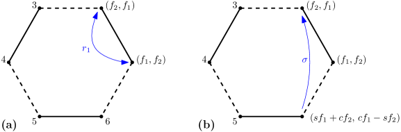
Figure 3.2. The graph from Example 3.2, its symmetries and the quotient with respect to representation (3.9). We use abbreviations $c=\cos\omega$ and $s=\sin\omega$.

The group $G=D_{3}$ has a unique two-dimensional irreducible representation $V_{\rho}:=\mathbb{C}^{2}$ given by

$$\sigma\mapsto\begin{pmatrix}\cos\omega&-\sin\omega\\ \sin\omega&\cos\omega\end{pmatrix},\qquad r_{1}\mapsto\begin{pmatrix}0&1\\ 1&0\end{pmatrix},\qquad r_{3}\mapsto\begin{pmatrix}\sin\omega&\cos\omega\\ \cos\omega&-\sin\omega\end{pmatrix},$$ (3.9)

where we included $r_{3}=r_{1}\sigma$ for future reference.

We will both describe the intertwiner space $\mathrm{Hom}_{G}(V_{\rho},V_{\pi})$ and compute the quotient operator $H_{\rho}$ using Definition 2.2. We will construct the intertwiner pictorially, see Fig. 3.3. An intertwiner $\phi\in\mathrm{Hom}_{G}(V_{\rho},V_{\pi})$ will be represented as a $6\times 2$ matrix and we will fill it up row by row. The first row are the free parameters,

$$\begin{pmatrix}\phi_{1,1}&\phi_{1,2}\end{pmatrix}=\begin{pmatrix}f_{1}&f_{2}\end{pmatrix}.$$ (3.10)

All other rows will be determined from the “representative” row (3.10) since all other vertices lie in the orbit of vertex 1 (the group action is transitive). We remark here that in more sophisticated examples, there may be dependencies among the entries of the representative row(s) if the corresponding vertex has a nontrivial stabilizer subgroup. We will encounter this in Example 3.3.

From the definition of the intertwiner, equation (2.9), and the action of $r_{1}$ on $V_{\pi}=\mathbb{C}^{6}$, we get

$$\phi_{2,\cdot}=(r_{1}\phi)_{1,\cdot}=\phi_{1,\cdot}r_{1}=\begin{pmatrix}f_{1}&f_{2}\end{pmatrix}\begin{pmatrix}0&1\\ 1&0\end{pmatrix}=\begin{pmatrix}f_{2}&f_{1}\end{pmatrix},$$ (3.11)

where $\phi_{j,\cdot}$ denotes the $j$-th row of $\phi$. This reasoning is schematically depicted in Fig. 3.3(a).

Figure 3.3. Construction of the intertwiner space in Example 3.2.

Similarly, using $\sigma$, we get

$$\phi_{6,\cdot}=(\sigma\phi)_{2,\cdot}=\phi_{2,\cdot}\sigma=\begin{pmatrix}f_{2}&f_{1}\end{pmatrix}\begin{pmatrix}\cos\omega&-\sin\omega\\ \sin\omega&\cos\omega\end{pmatrix}=\begin{pmatrix}sf_{1}+cf_{2}&cf_{1}-sf_{2}\end{pmatrix},$$ (3.12)

where we used abbreviations $c=\cos\omega$ and $s=\sin\omega$. This step is schematically depicted in Fig. 3.3(b).

Proceeding recursively, we find

$$\phi=\begin{pmatrix}f_{1}&f_{2}\\ f_{2}&f_{1}\\ cf_{1}-sf_{2}&sf_{1}+cf_{2}\\ cf_{2}-sf_{1}&sf_{2}+cf_{1}\\ sf_{2}+cf_{1}&cf_{2}-sf_{1}\\ sf_{1}+cf_{2}&cf_{1}-sf_{2}\end{pmatrix},$$ (3.13)

where $f_{1},f_{2}\in C$ are arbitrary constants.

To summarize, equation (3.13) parametrizes the space $\mathrm{Hom}_{G}(V_{\rho},V_{\pi})$. Choosing a basis, we can represent the action of $H$ on this space as a matrix (to obtain a Hermitian matrix, the basis should be orthonormal). But to understand the action of $H$, it is enough to focus our attention on the representative vertex and its neighbors, already determined in (3.11) and (3.12):

$$H\colon\begin{pmatrix}f_{1}&f_{2}\end{pmatrix}\quad\longmapsto\quad q\begin{pmatrix}f_{1}&f_{2}\end{pmatrix}+a\begin{pmatrix}f_{2}&f_{1}\end{pmatrix}+b\begin{pmatrix}sf_{1}+cf_{2}&cf_{1}-sf_{2}\end{pmatrix},$$ (3.14)

which corresponds to the graph in Fig. 3.2(c).

We now construct $H_{\rho}$ using Definition 2.2. There is only one orbit and we choose the vertex $1$ as the representative; namely, the fundamental domain is $\mathcal{D}=\{1\}$. The quotient operator $H_{\rho}$ consists of a single block $(1,1)$ of size $2\times 2$: since the group is fixed point free, $d_{1}=r=2$. Moreover, we can use equation (2.7) to determine its form. The only non-zero entries in the summation are $H_{1,1}$ (which corresponds to $g=e$), $H_{1,2}$ (with $g=r_{1}$) and $H_{1,6}$ (with $g=r_{3}$). Therefore the resulting quotient operator is

$$H_{\rho}=H_{1,1}e+H_{1,2}r_{1}+H_{1,6}r_{3}=\begin{pmatrix}q+b\sin\omega&a+b\cos\omega\\ a+b\cos\omega&q-b\sin\omega\end{pmatrix}.$$ (3.15)

For example, if we take $q=0$, $a=-1$ and $b=-2$, then the spectrum for the original matrix $H$ is

$$\mathrm{Spec}(H)=\{-3,\,-\sqrt{3},\,-\sqrt{3},\,\sqrt{3},\,\sqrt{3},\,3\},$$

while the matrix $H_{\rho}$ happens to be diagonal with entries $\pm\sqrt{3}$. That these eigenvalues are doubly degenerate in $\mathrm{Spec}(H)$ follow from Proposition 2.8. Explicitly, because $\deg\rho=2$, each eigenfunction of the quotient $H_{\rho}$ corresponds to a two-dimensional subspace of the eigenspace of $H$ with the same eigenvalue.

Example 3.3 (Disappearing vertices: vertices in the fundamental domain may not be equally represented in the quotient).

Here we study the quotients of the graph shown in Figure 1.1(a). It is invariant under the action of the symmetry group $G=S_{4}$, corresponding to the permutations of the vertices $1$, $2$, $3$ and $4$. The order of the group is $|S_{4}|=4!=24$ and it is generated by the three elements $(12)$, $(23)$ and $(34)$. The fundamental domain consists of the two vertices ‘$\bullet$’ and ‘$\circ$’ and their orbits with respect to the group action are $O_{\bullet}=\{1,\ldots,4$} and $O_{\circ}=\{5,\ldots,16\}$. We consider the operator $H$ on this graph given by

$$H_{ij}=\begin{cases}a&\mbox{if }i\sim j,\ \ i\in O_{\bullet},j\in O_{\circ}\mbox{ or }i\in O_{\circ},j\in O_{\bullet}\\ b&\mbox{if }i\sim j,\ \ i\in O_{\circ},j\in O_{\circ}\\ q_{\bullet}&\mbox{if }i=j\in O_{\bullet}\\ q_{\circ}&\mbox{if }i=j\in O_{\circ},\end{cases}$$ (3.16)

where $\sim$ indicates adjacency of the vertices. In this example, both the ‘$\bullet$’ and ‘$\circ$’ vertices have non-empty stabilizer groups. Choosing $1$ and $5$ as the orbit representatives (so that $\mathcal{D}=\{1,5\}$), we have $G_{\bullet}\cong S_{3}$ (permutations of vertices $2$, $3$ and $4$) and $G_{\circ}\cong S_{2}$ (permutations of vertices $3$ and $4$).

We now wish to find the quotient operator $H_{\rho}$ with respect to the so-called standard representation of $S_{4}$ given by

$$\rho_{(1\,2)}=\begin{pmatrix}0&-1&0\\ -1&0&0\\ 0&0&1\end{pmatrix},\quad\rho_{(2\,3)}=\begin{pmatrix}0&0&1\\ 0&1&0\\ 1&0&0\end{pmatrix},\quad\rho_{(3\,4)}=\begin{pmatrix}0&1&0\\ 1&0&0\\ 0&0&1\end{pmatrix}.$$ (3.17)

We start by determining the matrices $\Phi_{\circ}$ and $\Phi_{\bullet}$ consisting of orthonormal basis vectors for $(\textrm{V}_{\rho})^{G_{\circ}}$ and $(\textrm{V}_{\rho})^{G_{\bullet}}$, defined in equation (2.4). Note that it suffices to check the invariance condition $gv=v$ on the generators of these groups,

$$(\textrm{V}_{\rho})^{G_{\circ}} =\ker\left(\mathbb{\boldsymbol{I}}_{3}-\rho_{(3\,4)}\right)=\textrm{span}\left\{\begin{pmatrix}0\\ 0\\ 1\end{pmatrix},\begin{pmatrix}1\\ 1\\ 0\end{pmatrix}\right\},$$

$$(\textrm{V}_{\rho})^{G_{\bullet}} =\ker\left(\mathbb{\boldsymbol{I}}_{3}-\rho_{(3\,4)}\right)\bigcap\ker\left(\mathbb{\boldsymbol{I}}_{3}-\rho_{(2\,3)}\right)=\textrm{span}\left\{\begin{pmatrix}1\\ 1\\ 1\end{pmatrix}\right\},$$

and therefore

$$\Phi_{\circ}=\begin{pmatrix}0&1/\sqrt{2}\\ 0&1/\sqrt{2}\\ 1&0\end{pmatrix},\qquad\Phi_{\bullet}=\begin{pmatrix}1/\sqrt{3}\\ 1/\sqrt{3}\\ 1/\sqrt{3}\end{pmatrix}.$$ (3.18)

We proceed to finding the blocks of our quotient operator. Firstly we notice that $H_{1,g1}$ is only non-zero if $g\in G_{\bullet}$. Therefore we get

$$[H_{\rho}]_{\bullet,\bullet}=\frac{1}{\left|G_{\bullet}\right|}\sum_{g\in G_{\bullet}}\Phi_{\bullet}^{*}g\Phi_{\bullet}H_{\bullet,\bullet}=\Phi_{\bullet}^{*}\Phi_{\bullet}H_{\bullet,\bullet}=q_{\bullet},$$

where we used that $\Phi_{\bullet}$ is invariant under $g\in G_{\bullet}$. Similarly, we also have $H_{1,g5}\neq 0$ only if $g\in G_{\bullet}$. Therefore for the $1\times 2$ block $[H_{\rho}]_{\bullet,\circ}$ we obtain

$$[H_{\rho}]_{\bullet,\circ} =\frac{1}{\sqrt{\left|G_{\bullet}\right||G_{\circ}|}}\sum_{g\in G_{\bullet}}\Phi_{\bullet}^{*}g\Phi_{\circ}H_{\bullet,\circ}$$

$$=\frac{1}{\sqrt{\left|G_{\bullet}\right||G_{\circ}|}}\sum_{g\in G_{\bullet}}(g^{-1}\Phi_{\bullet})^{*}\Phi_{\circ}H_{\bullet,\circ}$$

$$=\frac{\sqrt{|G_{\bullet}|}}{\sqrt{|G_{\circ}|}}\left(\Phi_{\bullet}^{*}\Phi_{\circ}\right)H_{\bullet,\circ}=\frac{\sqrt{6}}{\sqrt{2}}\begin{pmatrix}1/\sqrt{3}&\sqrt{2/3}\end{pmatrix}a=\begin{pmatrix}a&a\sqrt{2}\end{pmatrix}.$$

Finally, the group elements contributing to the block $[H_{\rho}]_{\circ,\circ}$ according to (2.5) are $g=e$, $(3\,4)$, $(1\,2)$ and $(3\,4)(1\,2)$ (for all other $g$, $H_{5,g5}=0$). We split the summation into two parts and use the invariance properties

$$\rho_{(3\,4)}\Phi_{\circ}=\Phi_{\circ},\qquad\rho_{(3\,4)(1\,2)}\Phi_{\circ}=\rho_{(1\,2)}\Phi_{\circ}$$

to get

$$[H_{\rho}]_{\circ,\circ}=\frac{1}{|G_{\circ}|}\left(2\left(\Phi_{\circ}^{*}\Phi_{\circ}\right)q_{\circ}+2\left(\Phi_{\circ}^{*}\rho_{(1\,2)}\Phi_{\circ}\right)b\right)=\begin{pmatrix}q_{\circ}+b&0\\ 0&q_{\circ}-b\end{pmatrix}.$$

Collating all these blocks together we get

$$H_{\rho}=\begin{pmatrix}q_{\bullet}&a&a\sqrt{2}\\ a&q_{\circ}+b&0\\ a\sqrt{2}&0&q_{\circ}-b\end{pmatrix}.$$ (3.19)

It is interesting to observe that the vertices $\bullet$ and $\circ$ from the fundamental domain are not equally represented in the quotient operator (the vertex $\bullet$ partially disappeared, as $d_{\bullet}<r$). We will see below more quotients of this kind (and even a case when $\bullet$ disappears completely from the quotient when $d_{\bullet}=0$).

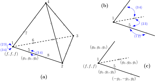
Figure 3.4. Computing the intertwiner rows in Example 3.3.

We can also work out the intertwiners pictorially, as in the previous examples; Figure 3.4 depicts the initial steps. We note that in the first step, we observe that the number of the free parameters describing the rows $\phi_{1,\cdot}$ and $\phi_{5,\cdot}$ are reduced because these rows must be invariant with respect to multiplication by $\rho_{(2\,3)},\rho_{(3\,4)}$ and $\rho_{(3\,4)}$ correspondingly. This step is analogous to finding the matrics $\Phi_{\bullet}$ and $\Phi_{\circ}$ in equation (3.18).

To give a numerical example, we take the standard Laplacian (corresponding to the choice $a=b=-1$, $q_{\bullet}=3$, $q_{\circ}=2$ in (3.16)), and get that the spectrum of the original operator $H$ is

$$\mathrm{Spec}(H)=\{0,\ 0.44,\ 0.44,\ 0.44,\ 1,\ 1,\ 2,\ 2,\ 2,\ 3,\ 3,\ 3,\ 4,\ 4.56,\ 4.56,\ 4.56\},$$ (3.20)

while the spectrum of $H_{\rho}$ picks out some triply degenerate eigenvalues

$$\mathrm{Spec}(H_{\rho})=\{0.44,\ 2,\ 4.56\}.$$

At this point we remark that the quotient $H_{\rho}$ is smaller than the graph announced in Example 1.1. Correspondingly, it does not capture all of the triply degenerate eigenvalues from (3.20). According to Proposition 2.8(2), $\mathrm{Spec}(H)$ is the union of spectra of all quotients with respect to the irreducible representations (and each eigenvalue is obtained with the multiplicity of the dimension of representation). The group $S_{4}$ has five irreducible representations. Two of them (including $\rho$ above) are three-dimensional, one is two-dimensional and two are one-dimensional. The latter two are the sign representation and the trivial representation.

The quotient with respect to the trivial representation is

$$H_{\mathrm{triv}}=\begin{pmatrix}q_{\bullet}&\sqrt{3}a\\ \sqrt{3}a&q_{\circ}+b\end{pmatrix}.$$ (3.21)

The same values for $q_{\circ},q_{\bullet},a$ and $b$ as before give the spectrum $\mathrm{Spec}(H_{\mathrm{triv}})=\{0,\ 4\}$.

The remaining eigenvalues in (3.20) are obtained from the 2d irrep $H_{\text{2d}}=q_{\circ}+b=(1)$, which captures the doubly degenerate eigenvalue $1$ in $\mathrm{Spec}(H)$, and the other 3d irrep of $S_{4}$, whose quotient

$$H_{\hat{\rho}}=q_{\circ}-b=(3)$$ (3.22)

captures the remaining triply degenerate eigenvalue in $\mathrm{Spec}(H)$. Note that in these instances we have $d_{\circ}=1$ and $d_{\bullet}=0$, which leads to the quotient operators being one-dimensional. Comparing again with Example 1.1, we note that the reflection symmetry in Fig. 1.1(b) allows to represent $H_{\sigma}$ in (1.3) as a direct sum $H_{\rho}\oplus H_{\hat{\rho}}$ of operators (3.19) and (3.22). A more direct way to obtain $H_{\sigma}$ is outlined in Example 4.11 — and it involves using a subgroup of $S_{4}$ rather than the full group of symmetries.

We have accounted for all the eigenvalues in (3.20) by examining the spectra of four quotients. However, $S_{4}$ has another irrep, the sign representation. A quick calculation shows that

$$d=\dim(\mathrm{Hom}_{G}(V_{\textrm{sgn}},\textrm{V}_{\pi}))=\frac{1}{|G|}\sum_{g\in G}\chi_{\textrm{sgn}}(g)\bar{\chi}_{\pi}(g)=0,$$

where the last equality results from Schur’s orthogonality relations and $\chi$ denote the characters of the corresponding representations. We could have also derived this by showing that $d_{\bullet}=d_{\circ}=0$. This means that there is no quotient operator $H_{\textrm{sgn}}$ and, indeed, there are no associated eigenvalues in $\mathrm{Spec}(H)$.

Example 3.4 (Directed graphs).

In all the previous examples in this section we have taken the $\pi$-symmetric operator T to be unitarily diagonalizable. However, Definition 2.2 of the quotient operator does not require this to be the case. Let us therefore take the following example, which is invariant under the symmetry group $C_{2}=\{e,\thinspace r\}$. The matrix T in (3.23) is invariant under the exchange of indices $3$ and $4$.

$$\textrm{T}=\begin{pmatrix}2&1&0&0\\ 1&2&0&0\\ 0&1&1&0\\ 0&1&0&1\end{pmatrix},\hskip 30.0pt\pi_{(3\,4)}=\begin{pmatrix}1&0&0&0\\ 0&1&0&0\\ 0&0&0&1\\ 0&0&1&0\end{pmatrix},\hskip 30.0pt\textrm{T}_{\mathrm{triv}}=\begin{pmatrix}2&1&0\\ 1&2&0\\ 0&\sqrt{2}&1\end{pmatrix}$$ (3.23)

The connections of T (the non-zero off-diagonal entries) can be interpreted in terms of the directed graph given in Figure 3.5 (a).

(a)                       (b)

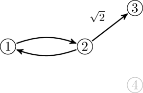
Figure 3.5. (a) Directed graph associated to the adjacency matrix T and (b) the directed graph associated to the quotient operator $\textrm{T}_{\rho}$.

If we select the fundamental domain to consist of the vertices $1,2$ and $3$ and choose the trivial representation then the formula (2.5) gives, for instance,

$$[\textrm{T}_{\mathrm{triv}}]_{32}=\frac{1}{\sqrt{|G_{2}||G_{3}|}}(\textrm{T}_{32}+\textrm{T}_{42})=\frac{2}{\sqrt{2}}=\sqrt{2}.$$

The complete matrix is displayed above in (3.23) and the corresponding graph is illustrated in Figure 3.5,(b). One sees immediately the resemblance between the original and quotient operators. Furthermore we have the decomposition into Jordan normal form of $\textrm{T}=PJP^{-1}$, where

$$P=\frac{1}{4}\begin{pmatrix}2&0&2&0\\ 2&0&-2&0\\ 1&-2&-1&0\\ 1&-2&-1&1\end{pmatrix}\hskip 50.0ptJ=\begin{pmatrix}3&0&0&0\\ 0&1&1&0\\ 0&0&1&0\\ 0&0&0&1\end{pmatrix}$$

and similarly for $\textrm{T}_{\mathrm{triv}}=QJ_{\mathrm{triv}}Q^{-1}$, where

$$Q=\frac{1}{4}\begin{pmatrix}2&0&2\\ 2&0&-2\\ \sqrt{2}&-2\sqrt{2}&-\sqrt{2}\end{pmatrix}\hskip 50.0ptJ_{\mathrm{triv}}=\begin{pmatrix}3&0&0\\ 0&1&1\\ 0&0&1\end{pmatrix}.$$

Hence both T and $\textrm{T}_{\mathrm{triv}}$ are non-diagonalizable. Nevertheless we see that the spectral relation (2.20) given in Proposition 2.8 still holds. For example, in this case, taking the spectral parameter $\lambda=1$ we have

$$\mathrm{Hom}_{G}(V_{\rho},\mathbf{E}_{1}^{\textrm{T}}(1))\cong\mathbf{E}_{1}^{\textrm{T}_{\rho}}(1).$$ (3.24)

Note that the $\lambda=1$ eigenspace of T is of dimension $2$ ($\dim\mathbf{E}_{1}^{\textrm{T}}(1)=2$), but there is only one eigenvector (up to scaling) in this eigenspace that transforms according to the trivial representation. This eigenvector is explicitly given as the second column of $P$ and it corresponds to the eigenvector of $\textrm{T}_{\mathrm{triv}}$ with the same eigenvalue (the second column of $Q$). Hence the vector spaces in (3.24) are one-dimensional.

Similarly, T has a $\lambda=1$ generalized eigenvector of rank $2$, which transforms under the trivial representation. This is the third column vector of $P$ which corresponds to the third column vector of $Q$. Namely, the second and third column vectors of $P$ span $\mathrm{Hom}_{G}(V_{\rho},\mathbf{E}_{2}^{\textrm{T}}(1))$ and similarly the second and third column vectors of $Q$ span the isomorphic space $\mathbf{E}_{2}^{\textrm{T}_{\rho}}(1)$.

Example 3.5 (The quaternion group).

The current example has some interesting physical content. Within quantum chaos, Gaussian Symplectic Ensembles (GSE) statistics have typically been associated with the distribution of energy levels in complex quantum systems possessing a half-integer spin. However, recently it has been demonstrated that one may still observe these statistics even without spin (i.e. the wavefunctions have a single component) [JMS14], leading to the first experimental realization of the GSE [RAJ⁺16]. The example in [JMS14] was achieved by obtaining a suitable quotient of a quantum graph with a symmetry corresponding to the quaternion group $Q_{8}$. Here we provide an analogous example using discrete graphs to highlight some interesting properties of this quotient operator.

The quaternion group is given by the following eight group elements

$$Q_{8}:=\{\pm 1,\pm\mathfrak{i},\pm\mathfrak{j},\pm\mathfrak{k}:\mathfrak{i}^{2}=\mathfrak{j}^{2}=\mathfrak{k}^{2}=\mathfrak{i}\mathfrak{j}\mathfrak{k}=-1\}$$

and can be generated by the two elements $\mathfrak{i}$ and $\mathfrak{j}$. We construct a discrete graph which is symmetric under the action of $Q_{8}$. The graph is shown in Figure 3.6 (a); it has 24 vertices and edge weights $a,b,c,d\in\mathbb{R}$ such that $a\neq b$ and $c\neq d$ (one may also include vertex potentials as long as the symmetry is retained). The graph is based on the Cayley graph of $Q_{8}$ with respect to the generating set $\{\mathfrak{i},\mathfrak{j}\}$ (see e.g. [JMS14]). To this Cayley graph we add a vertex at the middle of each edge, to obtain the graph in Figure 3.6 (a). We take a representation $V_{\pi}=\mathbb{C}^{24}$, which acts by permuting the eight vertices $\{\pm 1,~{}\pm\mathfrak{i},~{}\pm\mathfrak{j},~{}\pm\mathfrak{k}\}$ by left action and permuting all other vertices accordingly. There is a real-symmetric weighted adjacency matrix $A$ associated to the graph in 3.6 (a) and this operator $A$ is $Q_{8}$-symmetric.

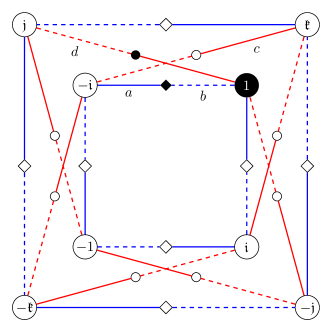
(a)        (b)

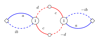
Figure 3.6. (a) Discrete graph with 24 vertices and edge weights $a,b,c$ and $d$ associated to blue solid, blue dashed, red solid and red dashed lines respectively. The vertices taken to form the fundamental domain are marked in black. (b) The quotient graph associated to the irreducible representation given in (3.25).

The irreducible representation of $Q_{8}$, in which we are interested, is generated by the following $2\times 2$ matrices

$$\mathfrak{i}\mapsto\begin{pmatrix}\mathrm{i}&0\\ 0&-\mathrm{i}\end{pmatrix},\hskip 30.0pt\mathfrak{j}\mapsto\begin{pmatrix}0&1\\ -1&0\end{pmatrix}.$$ (3.25)

We choose three vertices to form the fundamental domain under the group action (see the vertices marked in black in Figure 3.6 (a)). Using the formula (2.5) we obtain a quotient operator comprised of nine $2\times 2$ blocks, given by

$$A_{\rho}=\begin{pmatrix}0&a\mathbb{\boldsymbol{I}}_{2}+b\mathfrak{i}&c\mathbb{\boldsymbol{I}}_{2}+d\mathfrak{j}\\ a\mathbb{\boldsymbol{I}}_{2}+b\mathfrak{i}^{*}&0&0\\ c\mathbb{\boldsymbol{I}}_{2}+d\mathfrak{j}^{*}&0&0\end{pmatrix}.$$ (3.26)

One may, equally validly, view each of the 6 indices as separate vertices, in which case one has the corresponding graph shown in Figure 3.6,(b).

In contrast to the original operator $A$, the quotient operator $A_{\rho}$ is no longer real-symmetric. Instead, it is what is known as quaternion self-dual - a generalization of self-adjointness to quaternions. Specifically, a matrix $B$ is said to be quaternion self-dual if it has quaternion-real entries, i.e. $B_{nm}=a_{nm}^{(1)}1+a_{nm}^{(\mathfrak{i})}\mathfrak{i}+a_{nm}^{(\mathfrak{j})}\mathfrak{j}+a_{nm}^{(\mathfrak{k})}\mathfrak{k}$ where the $a_{i}$ are real coefficients, and $B_{mn}=\overline{B_{nm}}=a_{nm}^{(1)}1-a_{nm}^{(\mathfrak{i})}\mathfrak{i}-a_{nm}^{(\mathfrak{j})}\mathfrak{j}-a_{nm}^{(\mathfrak{k})}\mathfrak{k}$ for all $n,m$. Here, the $2\times 2$ blocks in $A_{\rho}$ are complex representations of quaternion-real elements and the quotient operator is quaternion self-dual since $g^{*}=-g$ for $g=\mathfrak{i},\mathfrak{j},\mathfrak{k}$. Interestingly, a quaternion-self dual matrix will have a two-fold degeneracy in the spectrum, which, in the physics literature, is known as Kramer’s degeneracy (see e.g. Chapter 2 of [Haa10]).

This difference in structure between the original operator $A$ and the quotient operator $A_{\rho}$ has important ramifications in quantum chaos. This is because (see e.g [Haa10] for more details) the statistical distribution of eigenvalues in quantum systems, whose classical counterparts are chaotic, typically align with the eigenvalues of the Gaussian Orthogonal Ensemble (GOE) when the operator is real-symmetric and the GSE when the operator is quaternion self-dual.

4. Quantum graph quotients

Differential operators on metric graphs, also known as “quantum graphs” arise in mathematical physics and spectral geometry either as standalone models of interest or as limits of operators on thin branching domains. We keep the description of quantum graphs below as condensed as possible. A reader who is unfamiliar with quantum graphs has many sources to choose from, in particular the elementary introduction [Ber17], the introductory exercises [BG18], the review [GS06] and the books [Pos12, BK13a, Mug14].

The Laplacian (or the Schrödinger operator) on a quantum graph is an unbounded operator on an infinite-dimensional Hilbert space and would not appear to fit within our current framework. However a quotient of a quantum graph has already been defined in [BPBS09, PB10] and in this section we show that we can indeed extend our methods to this setting. The result is a more explicit and compact construction than those given in Section 6 in [BPBS09] and Section 4.2 in [PB10]. Moreover, the quotient quantum graphs we obtain here are always self-adjoint — thus answering a question that was left open in [BPBS09, PB10].

4.1. Quantum graphs in a nutshell

Consider a graph $\Gamma$ with finite vertex and edge sets $\mathcal{V}$ and $\mathcal{E}$. If we associate a length $l_{e}>0$ to each edge $e\in\mathcal{E}$ the graph $\Gamma$ becomes a metric graph, which allows us to identify points $x\in[0,l_{e}]$ along each edge. To do this, we need to assign a direction to each edge which, at the moment, we can do arbitrarily.

We now consider functions and operators on the metric graph $\Gamma$. To this end we take our function space to be the direct sum of spaces of functions defined on each edge

$$L^{2}(\Gamma):=\oplus_{e\in\mathcal{E}}L^{2}(e):=\oplus_{e\in\mathcal{E}}L^{2}([0,l_{e}])\quad\mbox{and}\quad H^{2}(\Gamma):=\oplus_{e\in\mathcal{E}}H^{2}(e):=\oplus_{e\in\mathcal{E}}H^{2}([0,l_{e}])$$ (4.1)

and choose some Schrödinger type operator defined on $H^{2}(\Gamma)$,

$$\textrm{T}:=-\triangle+q\thinspace:\thinspace\begin{pmatrix}f_{e_{1}}\\ \vdots\\ f_{e_{|\mathcal{E}|}}\end{pmatrix}\mapsto\begin{pmatrix}-f_{e_{1}}^{\prime\prime}+q_{e_{1}}f_{e_{1}}\\ \vdots\\ -f_{e_{|\mathcal{E}|}}^{\prime\prime}+q_{e_{|\mathcal{E}|}}f_{e_{|\mathcal{E}|}}\end{pmatrix},$$ (4.2)

where $f_{e}$ is the component of a function $f$ on $\Gamma$ to the edge $e\in\mathcal{E}$.

To make the operator self-adjoint we must further restrict the domain of the operator by introducing vertex conditions, formulated in terms of the values of the functions and their derivatives at the edge ends. To formulate these conditions, we introduce the “trace” operators $\gamma_{D},\gamma_{N}:H^{2}(\Gamma)\to\mathbb{C}^{2|\mathcal{E}|}$ which extract the Dirichlet (value) and Neumann (derivative) boundary data from a function $f$ defined on a graph,

$$\gamma_{D}(f):=\begin{pmatrix}f_{e_{1}}(0)\\ f_{e_{1}}(l_{e_{1}})\\ \vdots\\ f_{e_{|\mathcal{E}|}}(0)\\ f_{e_{|\mathcal{E}|}}(l_{e_{|\mathcal{E}|}})\end{pmatrix}\quad\hbox{and}\quad\gamma_{N}(f):=\begin{pmatrix}f^{\prime}_{e_{1}}(0)\\ -f^{\prime}_{e_{1}}(l_{e_{1}})\\ \vdots\\ f^{\prime}_{e_{|\mathcal{E}|}}(0)\\ -f^{\prime}_{e_{|\mathcal{E}|}}(l_{e_{|\mathcal{E}|}})\end{pmatrix}\ ;$$ (4.3)

The vertex conditions are implemented by the condition

$$(A\thinspace|\thinspace B)\begin{pmatrix}\gamma_{D}(f)\\ \gamma_{N}(f)\end{pmatrix}=A\gamma_{D}(f)+B\gamma_{N}(f)=0,$$ (4.4)

where $A$ and $B$ are $2|\mathcal{E}|\times 2|\mathcal{E}|$ complex matrices. We shall write $\textrm{Dom}(\textrm{T})$ for the domain of our operator, i.e. the set of functions $f\in H^{2}(\Gamma)$ such that (4.4) is satisfied. The connectivity of the graph is retained by requiring that only values and/or derivatives at the points corresponding to the same vertex are allowed to enter any equation of conditions (4.4). In particular this means we have the decomposition $A=\bigoplus_{v\in\mathcal{V}}A^{(v)}$, and similarly for $B$. It was shown by Kostrykin and Schrader [KS99] that the operator is self-adjoint if and only if the following conditions hold

1. the $2|\mathcal{E}|\times 4|\mathcal{E}|$ matrix $(A|B)$ is of full rank, i.e. $\textrm{Rank}(A|B)=2|\mathcal{E}|$.

2. $AB^{*}$ is self adjoint.

Remark 4.1.

One obtains a unitarily equivalent quantum graph, specified by the conditions $\tilde{A}=CA$ and $\tilde{B}=CB$, if and only if $C\in GL(\mathbb{C}^{2|\mathcal{E}|})$, [KS99].

A compact quantum graph (i.e. a graph with a finite number of edges and a finite length for each edge) with bounded potential $q$ has a discrete infinite eigenvalue spectrum bounded from below, which we denote by

$$\mathrm{Spec}(\Gamma):=\left\{k^{2}\thinspace:\thinspace-\triangle f+qf=k^{2}f,\ (\gamma_{D}(f),\gamma_{N}(f))^{T}\in\ker(A|B)\right\}.$$ (4.5)

A common choice of vertex conditions are Kirchhoff–Neumann conditions: for every vertex the values at the edge-ends corresponding to this vertex are the same and the derivatives (with the signs given in (4.3)) add up to zero. In particular, at a vertex of degree 2 these conditions are equivalent to requiring that the function is $C^{1}$ across the vertex. Conversely, each point on an edge may be viewed as a “dummy vertex” of degree 2 with Neumann-Kirchhoff conditions.

4.2. Quantum graphs and symmetry

We now extend the notion of a $G$-symmetric operator (Definition 2.1) to quantum graphs. To motivate our definition informally consider a graph $\Gamma$ with some symmetries: transformations on the metric graph that map vertices to vertices while preserving the graph’s metric structure. We can assume, without loss of generality, that an edge is never mapped to its own reversal. If this condition is satisfied, it is easy to see that the edge directions (as described in Section 4.1) may be assigned so that they are preserved under the action of the symmetry group. From now on we will denote by $ge=e^{\prime}$ the action of an element $g$ of the symmetry group $G$ on the edges with their assigned direction. Now the “preservation of metric structure” mentioned above is simply the condition that the edge lengths are fixed by all $g\in G$, i.e. $l_{ge}=l_{e}$. This allows us to pointwise compare functions defined on two $G$-related edges. We are now ready to introduce the notion of a $G$-symmetric quantum graph.

Definition 4.2.

Let $\textrm{V}_{\pi}:=\mathbb{C}^{\mathcal{E}}$ be the vector space of functions $\mathcal{E}\to\mathbb{C}$ and let $\pi:G\rightarrow\textrm{GL}(\textrm{V}_{\pi})$ be a group homomorphism such that for each $g\in G$, $\pi(g)$ is a permutation matrix. A quantum graph $(\Gamma,T)$ is $G$-symmetric (with respect to the representation $\pi$) if for all $g\in G$

1. the edge lengths are preserved: $l_{ge}=l_{e}$ for all $e\in\mathcal{E}$,

2. the potential is preserved: $q_{ge}\equiv q_{e}$ for all $e\in\mathcal{E}$,

3. the operator domain is preserved:

   $$f=\begin{pmatrix}f_{e_{1}}\\ \vdots\\ f_{e_{|\mathcal{E}|}}\end{pmatrix}\in\textrm{Dom}(\textrm{T})\qquad\Leftrightarrow\qquad\pi(g)f:=\begin{pmatrix}f_{g^{-1}e_{1}}\\ \vdots\\ f_{g^{-1}e_{|\mathcal{E}|}}\end{pmatrix}\in\textrm{Dom}(\textrm{T}).$$ (4.6)

Some comments are in order. Since $l_{e}=l_{ge}$, there is a natural isomorphism $H^{2}(e)\cong H^{2}(ge)$ for every $g\in G$. This allows us to define the action of $\pi(g)$ on the function space $H^{2}(\Gamma)$ (or any other similar space on $\Gamma$) as in the right-hand side of (4.6). Informally, this just means that the transformation $\pi(g)$ takes the function from an edge $e$ and places it on the edge $ge$. In “placing” the function, we implicitly use the isomorphism mentioned above. In particular, the condition on the potential $q=(q_{e_{1}},\ldots,q_{e_{|\mathcal{E}|}})^{T}$ in Definition 4.2 can be now written as $\pi(g)q=q$ for any $g\in G$.

We note that the action of $\pi(g)$ above coincides with the result of the formal multiplication of the vector $f$ by the permutation matrix $\pi(g)$. This multiplication is “formal” because different entries of $f$ belong to different spaces and there is no a priori way to shuffle them or create linear combinations. It is only through symmetry of the graph and the resulting isomorphism between different edge spaces that we get a meaningful result. We will return to this point in the proof of Theorem 4.7 below.

As a corollary of the discussion above we get that if $\Gamma$ is a $G$-symmetric graph (with respect to a representation $\pi$) then the function spaces $L^{2}(\Gamma)$ and $H^{2}(\Gamma)$ are $G$-modules, and so is also $\textrm{Dom}(\textrm{T})\subset H^{2}(\Gamma)$.

Moving on to the requirement on the domain of $T$, one can easily check that

$$\gamma_{D}(\pi(g)f)=\hat{\pi}(g)\gamma_{D}(f),\qquad\text{where }\hat{\pi}(g):=\pi(g)\otimes\mathbb{\boldsymbol{I}}_{2},$$ (4.7)

and similarly for the Neumann trace, $\gamma_{N}$. In view of description (4.4) of the domain $\textrm{Dom}(T)$, condition (4.6) is equivalent to

$$AF+BF^{\prime}=0\qquad\Leftrightarrow\qquad A\hat{\pi}(g)F+B\hat{\pi}(g)F^{\prime}=0\qquad\text{for all }g\in G\text{ and }F,F^{\prime}\in\mathbb{C}^{2|\mathcal{E}|}.$$ (4.8)

Finally, we remark that, in general, the matrices $A$ and $B$ are not $G$-symmetric (see Example 4.9). But there is always an equivalent choice that is $G$-symmetric (with respect to the permutation representation $\hat{\pi}$).

Lemma 4.3.

Let $A$ and $B$ define vertex conditions on a $G$-symmetric quantum graph. Then the matrices

$$\widetilde{A}=(A+\mathrm{i}B)^{-1}A\qquad\mbox{and}\qquad\widetilde{B}=(A+\mathrm{i}B)^{-1}B.$$ (4.9)

define equivalent vertex conditions. Furthermore, $\widetilde{A}$ and $\widetilde{B}$ are $G$-symmetric, i.e.,

$$\widetilde{A}\hat{\pi}(g)=\hat{\pi}(g)\widetilde{A}\qquad\mbox{and}\qquad\widetilde{B}\hat{\pi}(g)=\hat{\pi}(g)\widetilde{B}\qquad\text{for all }g\in G.$$ (4.10)

Proof.

It is shown in [KS99] (see also [BK13a, lemma 1.4.7]) that the matrix $A+\mathrm{i}B$ is invertible. Therefore (see Remark 4.1) $\widetilde{A}$ and $\widetilde{B}$ define equivalent vertex conditions. To show (4.10) we observe that since $\widetilde{A}+\mathrm{i}\widetilde{B}=\mathbb{\boldsymbol{I}}$ commutes with $\hat{\pi}(g)$ for any $g\in G$, it is enough to show that $\widetilde{A}-\mathrm{i}\widetilde{B}$ also commutes with $\hat{\pi}(g)$ for any $g\in G$.

Take an arbitrary vector $a\in\mathbb{C}^{2|\mathcal{E}|}$ and let

$$b=(\widetilde{A}-\mathrm{i}\widetilde{B})a.$$ (4.11)

Writing out the definitions of $\widetilde{A}$ and $\widetilde{B}$ from (4.9) and using (4.8) we get for all $g\in G$

$$b=(\widetilde{A}-\mathrm{i}\widetilde{B})a~{}~{} \Leftrightarrow~{}~{}b=(A+\mathrm{i}B)^{-1}(A-\mathrm{i}B)a$$

$$\Leftrightarrow A(b-a)+B(\mathrm{i}b+\mathrm{i}a)=0$$

$$\Leftrightarrow A\hat{\pi}(g)(b-a)+B\hat{\pi}(g)(\mathrm{i}b+\mathrm{i}a)=0$$

$$\Leftrightarrow(A\hat{\pi}(g)+\mathrm{i}B\hat{\pi}(g))b=(A\hat{\pi}(g)-\mathrm{i}B\hat{\pi}(g))a$$

$$\Leftrightarrow b=\hat{\pi}(g)^{*}(A+\mathrm{i}B)^{-1}(A-\mathrm{i}B)\hat{\pi}(g)a.$$

We conclude that for every $a$

$$(\widetilde{A}-\mathrm{i}\widetilde{B})a=\hat{\pi}(g)^{*}(\widetilde{A}-\mathrm{i}\widetilde{B})\hat{\pi}(g)a,$$ (4.12)

which establishes the desired invariance. ∎

Remark 4.4.

In equation (4.4), the rows of $A$ and $B$ correspond to the restrictions imposed on the domain of the operator. Unlike the columns of $A$ and $B$, the rows sre not a priori related to any particular location in the graph.

Once symmetrized by (4.9), $\widetilde{A}$ and $\widetilde{B}$ can be properly viewed as operators on $\mathbb{C}^{\mathcal{E}}\otimes\mathbb{C}^{2}=\mathbb{C}^{2|\mathcal{E}|}$. The latter space is a $G$-module with $g$ acting by $\pi(g)\otimes\mathbb{\boldsymbol{I}}_{2}$. When $\widetilde{A}$ and $\widetilde{B}$ are $G$-symmetric, we can take their quotient with respect to a representation $\textrm{V}_{\rho}$.

From now on we will assume that our chosen $A$ and $B$ have already been symmetrized using (4.9). Their rows and columns will be labeled by the index set $\big{\{}1,\emph{$\overline{1}$},2,\emph{$\overline{2}$},\ldots|\mathcal{E}|,\emph{$\overline{|\mathcal{E}|}$}\big{\}}$. We will also use the following notation for $2\times 2$ blocks of $A$ corresponding to edges $e_{i}$, $e_{j}$:

$$A_{i,j}^{\otimes}=\begin{pmatrix}A_{i,j}&A_{i,\emph{$\overline{j}$}}\\ A_{\emph{$\overline{i}$},j}&A_{\emph{$\overline{i}$}\emph{$\overline{j}$}}\end{pmatrix},$$ (4.13)

and similarly for $B$.

4.3. Quotient quantum graph

We start from a graph $\Gamma$ with a corresponding operator $\textrm{T}:\textrm{Dom}(\textrm{T})\to L^{2}(\Gamma)$ which is $G$-symmetric. For any $G$-module $\textrm{V}_{\rho}$ we will describe a new graph $\Gamma_{\rho}$ with a corresponding operator $\textrm{T}_{\rho}$ (see Definition 4.5 below). In Theorem 4.7 we will see that $\textrm{T}_{\rho}$ is self-adjoint and unitarily equivalent to $\left.T\right|_{\mathrm{Hom}_{G}(\textrm{V}_{\rho},\textrm{Dom}(\textrm{T}))}$, which is analogous to Theorem 2.5 for discrete graph operators.

As described in the previous subsection, both $\textrm{Dom}(\textrm{T})$ and $L^{2}(\Gamma)$ are $G$-modules. Since $G$ acts on the edge set $\mathcal{E}$ of $\Gamma$ (this action is given by the permutation representation $\pi$), we may choose a fundamental domain $\mathcal{D}=\{e_{1},e_{2}\ldots,e_{|\mathcal{D}|}\}$ by selecting precisely one edge $e_{i}$ from each orbit $O_{i}=\{e_{k}\in\mathcal{E}:\exists g\in G,e_{k}=ge_{i}\}$. For each $e_{i}\in\mathcal{D}$, consider the stabilizer group $G_{i}=\left\{g\in G~{}:~{}ge_{i}=e_{i}\right\}$ and $(\textrm{V}_{\rho})^{G_{i}}$, the $G_{i}$-invariant subspace of $\textrm{V}_{\rho}$. Denote $d_{i}:=\dim(\textrm{V}_{\rho})^{G_{i}}$ and take $d_{i}$ copies of the directed edge $e_{i}$, i.e., these are $d_{i}$ intervals, each of length $l_{e_{i}}$. Denote these by $\{e_{i,j}\}_{j=1,\ldots,d_{i}}$. Furthermore, assume that the matrices $A,~{}B$ describing the vertex conditions of $\Gamma$ are $G$-symmetric with respect to the permutation representation $\hat{\pi}(g)=\pi(g)\otimes\mathbb{\boldsymbol{I}}_{2}$ (see Lemma 4.3).

Definition 4.5 (Quotient quantum graph).

Let $(\Gamma,T)$ be a $G$-symmetric quantum graph, where $G$ is a finite group and let $\textrm{V}_{\rho}$ be a $G$-module. Referring to the description before this definition, we define the quotient graph $\Gamma_{\rho}$ to be a metric graph formed from the edges $\{e_{i,j}\colon e_{i}\in\mathcal{D},\ j=1,\ldots,d_{i}\}$ of length $l_{e_{i,j}}=l_{e_{i}}$. We define the operator $\textrm{T}_{\rho}$ by the differential expression $-d^{2}/dx^{2}+q_{e_{i}}$ acting on the edge $e_{i,j}$, with the vertex conditions specified by the matrices $A_{\rho}$ and $B_{\rho}$, which are the quotients of $A$ and $B$ by $\textrm{V}_{\rho}$.

Remark 4.6.

To give an explicit description of $A_{\rho}$ and $B_{\rho}$, we recall formula (2.5). For each $e_{i}\in\mathcal{D}$ pick $\{\varphi_{i}^{(n)}\}_{n=1}^{d_{i}}$ to be an orthonormal basis for $(\textrm{V}_{\rho})^{G_{i}}$ and form an $r\times d_{i}$ matrix $\Phi_{i}$ whose columns are these basis vectors ($r=\dim\rho$). With respect of the action of $G$ on $\mathbb{C}^{2|\mathcal{E}|}=\textrm{V}_{\pi}\otimes\mathbb{C}^{2}$, we note that $G_{i}=G_{\emph{$\overline{i}$}}$ and therefore $d_{i}=d_{\emph{$\overline{i}$}}$ and $\Phi_{i}=\Phi_{\emph{$\overline{i}$}}$.

Now, $A_{\rho}$ and $B_{\rho}$ are matrices comprised of $2|\mathcal{D}|\times 2|\mathcal{D}|$ blocks with the $(z,w)$-th block, $z,w\in\big{\{}1,\emph{$\overline{1}$},\ldots,|\mathcal{D}|,\emph{$\overline{|\mathcal{D}|}$}\big{\}}$, being the following $d_{z}\times d_{w}$ matrix

$$\left[A_{\rho}\right]_{z,w} =\frac{1}{\sqrt{|G_{z}||G_{w}|}}\Phi_{z}^{*}\,\left(\sum_{g\in G}A_{z,gw}\,g\right)\,\Phi_{w}$$ (4.14)

$$\left[B_{\rho}\right]_{z,w} =\frac{1}{\sqrt{|G_{z}||G_{w}|}}\Phi_{z}^{*}\,\left(\sum_{g\in G}B_{z,gw}\,g\right)\,\Phi_{w}.$$ (4.15)

Due to the order we assume on the entries of the boundary data in (4.3), the blocks computed in (4.14) and (4.15) are not contiguous within the matrices $A_{\rho}$ and $A_{\rho}$. To overcome this problem, we can instead use the notation introduced in (4.13) and write

$$\left[A_{\rho}\right]_{i,j}^{\otimes}=\frac{1}{\sqrt{|G_{i}||G_{j}|}}\sum_{g\in G}\left(\Phi_{i}^{*}g\Phi_{j}\right)\otimes A_{i,gj}^{\otimes}\qquad\left[B_{\rho}\right]_{i,j}^{\otimes}=\frac{1}{\sqrt{|G_{i}||G_{j}|}}\sum_{g\in G}\left(\Phi_{i}^{*}g\Phi_{j}\right)\otimes B_{i,gj}^{\otimes},$$ (4.16)

where $i,j\in\{1,2,\ldots,|\mathcal{D}|\}$. In Example 4.9 we will use this formula to compute the quotient.

The operator $\textrm{T}_{\rho}$ defined above plays the same role as the discrere graph quotient operator in Definition 2.2. To see this we note that if $\textrm{V}_{\rho}$ is a $G$-module then T acts on elements of $\mathrm{Hom}_{G}(\textrm{V}_{\rho},\textrm{Dom}(\textrm{T}))$ by composition and returns elements of $\mathrm{Hom}_{G}(\textrm{V}_{\rho},L^{2}(\Gamma))$ (see (2.11),(2.12) for the finite dimensional case). The space $\mathrm{Hom}_{G}(\textrm{V}_{\rho},\textrm{Dom}(\textrm{T}))$ warrants a deeper discussion as it is useful in computational examples (see Example 4.10). It consists of the row vectors $\phi=\left(\phi^{(1)},\ldots,\phi^{(r)}\right)$, $\phi^{(j)}\in\textrm{Dom}(\textrm{T})$, $j=1,\ldots,r=\dim(\textrm{V}_{\rho})$, satisfying the intertwining condition

$$\pi(g)\phi:=\left(\pi(g)\phi^{(1)},\ldots,\pi(g)\phi^{(r)}\right)=\phi g,\qquad\forall\ g\in G,$$ (4.17)

where each $\phi^{(j)}$ can be visualized as a column

$$\phi^{(j)}=\begin{pmatrix}\phi_{e_{1}}^{(j)},\\ \vdots\\ \phi_{e_{|\mathcal{E}|}}^{(j)}\end{pmatrix},\qquad\phi_{e_{k}}^{(j)}\in H^{2}([0,l_{e_{k}}]).$$

The action $\pi(g)\phi^{(j)}$ is defined in (4.6), while $g$ on the right-hand side of (4.17) denotes the action of $g$ on $\textrm{V}_{\rho}$.

The space $\mathrm{Hom}_{G}(\textrm{V}_{\rho},L^{2}(\Gamma))$ is defined analogously. The Hilbert space structure on

$\mathrm{Hom}_{G}(\textrm{V}_{\rho},L^{2}(\Gamma))$ is given by the Frobenius inner product

$$\langle\phi,\psi\rangle_{\mathrm{Hom}_{G}(\textrm{V}_{\rho},L^{2}(\Gamma))}=\textrm{Tr}\left(\phi^{*}\psi\right):=\sum_{j=1}^{r}\sum_{e\in\mathcal{E}}\langle\phi_{e}^{(j)},\psi_{e}^{(j)}\rangle_{L^{2}([0,l_{e}])}.$$ (4.18)

The action of $T$ mentioned above is

$$T:\mathrm{Hom}_{G}(\textrm{V}_{\rho},\textrm{Dom}(\textrm{T}))\to\mathrm{Hom}_{G}(\textrm{V}_{\rho},L^{2}(\Gamma))\qquad T:\left(\phi^{(1)},\ldots,\phi^{(r)}\right)\mapsto\left(T\phi^{(1)},\ldots,T\phi^{(r)}\right).$$ (4.19)

For this operator, which we denote by $T\big{|}_{\mathrm{Hom}_{G}(\textrm{V}_{\rho},\textrm{Dom}(\textrm{T}))}$, we have the following.

Theorem 4.7.

Let $G$ be a finite group, $(\Gamma,T)$ be a $G$-symmetric quantum graph (with the operator $T$ being self-adjoint) and let $\textrm{V}_{\rho}$ be a $G$-module. Then the operator $\textrm{T}_{\rho}$ is self-adjoint and is unitarily equivalent to $\left.T\right|_{\mathrm{Hom}_{G}(\textrm{V}_{\rho},\textrm{Dom}(\textrm{T}))}$.

The proof of Theorem 4.7 follows the spirit of the proof of Theorem 2.5, but has more technicalities due to the intertwiners being linear maps into an infinite dimensional space. For this reason we defer it to Appendix B.

Theorem 4.7 shows that the quotient quantum graph we describe in Definition 4.5 is also a quotient quantum graph according to [PB10, Definition 1]. There are several advantages to the quotient construction in Definition 4.5. The first is that the construction method of the quotient is simpler to implement and convenient for computer-aided computation (by employing the formulas (4.14),(4.15)). Another advantage is that our present construction ensures the self-adjointness of the operator on the quotient graph and by this answers a question which was left open in [BPBS09, PB10]. In addition, it is possible to construct quotients for general Schrödinger operators and not just the Laplacian. Finally, our construction extends to an alternative description of quantum graphs by scattering matrices, as detailed in the next section.

Note that the graph topology is described indirectly by the vertex conditions, which are implemented through $A_{\rho}$ and $B_{\rho}$. That these matrices satisfy the conditions reviewed in Section 4.1 is established in Lemma B.5.

4.4. Bond scattering matrix and quotients

The Schrödinger operator of a quantum graph is not a finite dimensional operator. However, there exists a so-called unitary evolution operator $U(k)=T(k)S(k)$ of finite dimension (equal to $2|\mathcal{E}|\times 2|\mathcal{E}|$) that can fully describe the spectrum. Here $T(k)$ is a bond transmission matrix and $S(k)$ a bond scattering matrix expressed in terms of the vertex condition matrices,

$$\forall k\in\mathbb{R},\quad\quad~{}~{}~{}S(k)=-\left(A+\mathrm{i}kB\right)^{-1}\left(A-\mathrm{i}kB\right)J,$$ (4.20)

where

$$J=\mathbb{\boldsymbol{I}}_{|\mathcal{E}|}\otimes\left(\begin{smallmatrix}0&1\\ 1&0\end{smallmatrix}\right),$$ (4.21)

is a matrix that swaps between entries corresponding to start-points and end-points of edges. Note that (4.20) is well defined, as it is shown in [KS99] (see also [BK13a, lemma 1.4.7]) that the matrix $A+\mathrm{i}kB$ is invertible.

The matrix $S(k)$ is assured to be unitary if the operator is self-adjoint, namely, if $(A|B)$ is of full rank and $AB^{*}$ is self adjoint [BK13a, lemma 1.4.7]. In addition, it might happen that $S(k)$ is $k$-independent. This occurs, for example, when the vertex conditions are either Kirchhoff-Neumann (see Example 4.9) or Dirichlet (a vertex with Dirichlet condition means that the function vanishes at that vertex).

To understand the physical meaning of $S(k)$ recall that its rows and columns are indexed by the set $\{1,\emph{$\overline{1}$},\ldots,|\mathcal{E}|,\emph{$\overline{|\mathcal{E}|}$}\}$. We view $j$ as corresponding to a wave traveling along the edge $e_{j}$ in the direction we assigned to $e_{j}$ and $\overline{j}$ as corresponding to the wave travelling against the assigned direction. The entry $[S(k)]_{z,z^{\prime}}$ then gives the quantum amplitude of wave scattering from the direction $z^{\prime}$ to direction $z$. In particular, $[S(k)]_{z,z^{\prime}}\neq 0$ only if $z^{\prime}$ is directed into some vertex $v$ and $z$ is directed out of $v$. The matrix $S(k)$ therefore contains all the information about the graph’s connectivity and its vertex conditions.

In contrast, the transmission matrix $T(k)$ is a diagonal matrix describing the wave evolution along the edges (in or against the assigned direction). When the potential $q$ is zero, $T(k)=e^{ik\hat{L}}$, where $\hat{L}:=\textrm{diag}(l_{e_{1}},l_{e_{1}},\ldots,l_{e_{|\mathcal{E}|}},l_{e_{|\mathcal{E}|}})$ is a diagonal matrix of edge lengths, each listed twice (for the two directions). The spectrum of the Laplacian (4.5) is then given by

$$\mathrm{Spec}(\Gamma)=\left\{k^{2}\colon\det\left(\mathbb{\boldsymbol{I}}_{2|\mathcal{E}|}-U\left(k\right)\right)=0\right\}\ ,$$ (4.22)

as was shown in [vB85, KS97] (see also [BK13a, Theorem 2.1.8]).

We may apply the theory of the current paper to compute the quotient of the graph’s scattering matrix. One then finds that taking the quotient operator of the scattering matrix equals the scattering matrix of the quotient graph. For simplicity we assume that the potential $q$ is zero.

Proposition 4.8.

Let $(\Gamma,T)$ be a $G$-symmetric quantum graph with zero potential, whose bond scattering matrix is denoted by $S(k)$. Let $\textrm{V}_{\rho}$ be a $G$-module and $(\Gamma_{\rho},T_{\rho})$ be the corresponding quotient graph as in Definition 4.5.

Then, for all $k\in\mathbb{C}$, $S(k)$ and $U(k)$ are $G$-symmetric, i.e.,

$$\forall g\in G;\qquad S(k)\hat{\pi}(g)=\hat{\pi}(g)S(k)\qquad\mbox{and}\qquad U(k)\hat{\pi}(g)=\hat{\pi}(g)U(k).$$ (4.23)

In addition, the scattering matrix of $(\Gamma_{\rho},T_{\rho})$ is given by the quotient operator $S_{\rho}(k)$ and the unitary evolution operator of $(\Gamma_{\rho},T_{\rho})$ is given by the quotient $U_{\rho}(k)$.

The proof of this Proposition is given in Appendix B.3.

We end by pointing out that there is another meaning to the notion ‘scattering matrix of a quantum graph’. This other scattering matrix is formed by connecting semi-infinite leads to some of the graph vertices. The dimension of this matrix is equal to the number of leads and each of its entries equals the probability amplitude for a wave to scatter from a certain lead to another. This amplitude is calculated by summing over all possible paths through the graph leading from the first lead to the second (including a direct transmission of the wave from the first lead to the second, if it exists). This matrix is sometimes called an exterior scattering matrix (to distinguish it from the edge-scattering matrix discussed above). More on this matrix can be found in [BBS12, KS03].

If a graph $\Gamma$ is $G$-symmetric and leads are attached to it in a way which respects this symmetry, then the obtained exterior scattering matrix, $\Sigma(k)$ inherits this symmetry. As a consequence, we are able to construct a quotient of this scattering matrix with respect to a representation $\rho$ of the symmetry group $G$. This quotient matrix, $\Sigma_{\rho}(k)$ was shown in [BSS10] to equal the exterior scattering matrix of the quotient graph $\Gamma_{\rho}$, with an appropriate connection of leads. Hence, the quotient theory in the current paper may be used to recover the previously obtained results in [BSS10].

4.5. Quotient quantum graph examples

Example 4.9.

Let $\Gamma$ be a star graph with three edges, one edge of length $l_{1}$ and the other two of length $l_{2}$ (see Figure 4.1 (a)). Equip all graph vertices with Neumann conditions. We observe that the graph is symmetric with respect to exchanging the two edges with the same length, i.e. $e_{2}\leftrightarrow e_{3}$. Hence, the symmetry group we take is $C_{2}=\{\mathrm{I},\mathrm{R}:\mathrm{R}^{2}=\mathrm{I}\}$, and the graph is $\pi$ symmetric, where the representation $\pi$ is

$$\pi(\mathrm{I})=\mathbb{\boldsymbol{I}}_{3},\hskip 50.0pt\pi(\mathrm{R})=\left(\begin{smallmatrix}1&0&0\\ 0&0&1\\ 0&1&0\end{smallmatrix}\right).$$

(a)        (b)

Figure 4.1. (a) A star graph $\Gamma$ with $C_{2}$ symmetry. (b) The corresponding quotient graph $\Gamma_{\rho}$ with respect to the trivial representation $\rho=\mathrm{V_{triv}}$. Its vertex conditions are given in (4.27).

The vertex conditions of the graph may be described by (using the notational convention as in (4.4)):

$$A=\left(\begin{smallmatrix}1&0&-1&0&0&0\\ 0&0&1&0&-1&0\\ 0&0&0&0&0&0\\ 0&0&0&0&0&0\\ 0&0&0&0&0&0\\ 0&0&0&0&0&0\end{smallmatrix}\right),\hskip 50.0ptB=\left(\begin{smallmatrix}0&0&0&0&0&0\\ 0&0&0&0&0&0\\ 1&0&1&0&1&0\\ 0&1&0&0&0&0\\ 0&0&0&1&0&0\\ 0&0&0&0&0&1\end{smallmatrix}\right),$$

Those matrices are not $\hat{\pi}$-symmetric (e.g., $A\hat{\pi}(R)\neq\hat{\pi}(R)A$). With the aid of Lemma 4.3 we replace those by the following $\hat{\pi}$-symmetric matrices which describe equivalent vertex conditions:

$$\widetilde{A}=(A+\mathrm{i}B)^{-1}A=\frac{1}{3}\left({\scriptsize\begin{array}[]{cc|cc|cc}2&0&-1&\,0&-1&0\\ 0&0&0&0&0&0\\ \hline\cr\rule{0.0pt}{8.0pt}-1&0&2&0&-1&0\\ 0&0&0&0&0&0\\ \hline\cr\rule{0.0pt}{8.0pt}-1&0&-1&0&2&0\\ 0&0&0&0&0&0\end{array}}\right),\qquad\widetilde{B}=(A+\mathrm{i}B)^{-1}B=\frac{1}{3i}\left({\scriptsize\begin{array}[]{cc|cc|cc}1&0&1&0&1&0\\ 0&3&0&0&0&0\\ \hline\cr\rule{0.0pt}{8.0pt}1&0&1&0&1&0\\ 0&0&0&3&0&0\\ \hline\cr\rule{0.0pt}{8.0pt}1&0&1&0&1&0\\ 0&0&0&0&0&3\end{array}}\right),$$

where the partitioning is added to align with block notation (4.13).

We are now in a position to construct the quotient graph $\Gamma_{\rho}$, and choose to do it for $\rho=\mathrm{V_{triv}}$, the trivial representation of $C_{2}$. We choose our fundamental domain to be $\mathcal{D}=\{e_{1},e_{2}\}$, with $e_{2}$ being a representative of the orbit $O_{e_{2}}=\{e_{2},e_{3}\}$.

We have $|G_{1}|=2$ and $|G_{2}|=1$, as well as $\Phi_{1}=\Phi_{2}=1$. Using (4.16), we get

$$\left[A_{\rho}\right]_{1,1}^{\otimes} =\frac{1}{2}\left[A_{1,1}^{\otimes}+A_{1,1}^{\otimes}\right]=\frac{1}{2}\left[\left(\begin{smallmatrix}2&0\\ 0&0\end{smallmatrix}\right)+\left(\begin{smallmatrix}2&0\\ 0&0\end{smallmatrix}\right)\right]=\left(\begin{smallmatrix}2&0\\ 0&0\end{smallmatrix}\right),$$ (4.24)

$$\left[A_{\rho}\right]_{1,2}^{\otimes} =\frac{1}{\sqrt{2}}\left[A_{1,2}^{\otimes}+A_{1,3}^{\otimes}\right]=\frac{1}{\sqrt{2}}\left[\left(\begin{smallmatrix}-1&0\\ 0&0\end{smallmatrix}\right)+\left(\begin{smallmatrix}-1&0\\ 0&0\end{smallmatrix}\right)\right]=\left(\begin{smallmatrix}-\sqrt{2}&0\\ 0&0\end{smallmatrix}\right)=\left[A_{\rho}\right]_{2,1}^{\otimes},$$ (4.25)

$$\left[A_{\rho}\right]_{2,2}^{\otimes} =\left[A_{2,2}^{\otimes}+A_{2,3}^{\otimes}\right]=\left[\left(\begin{smallmatrix}2&0\\ 0&0\end{smallmatrix}\right)+\left(\begin{smallmatrix}-1&0\\ 0&0\end{smallmatrix}\right]\right)=\left(\begin{smallmatrix}1&0\\ 0&0\end{smallmatrix}\right).$$ (4.26)

Performing the same computations for $B_{\rho}$, we obtain, altogether,

$$A_{\rho}=\frac{1}{3}\left(\begin{array}[]{cc|cc}2&0&-\sqrt{2}&0\\ 0&0&0&0\\ \hline\cr\rule{0.0pt}{14.0pt}-\sqrt{2}&0&1&0\\ 0&0&0&0\end{array}\right),\hskip 20.0ptB_{\rho}=\frac{1}{3i}\left(\begin{array}[]{cc|cc}1&0&\sqrt{2}&0\\ 0&3&0&0\\ \hline\cr\rule{0.0pt}{14.0pt}\sqrt{2}&0&2&0\\ 0&0&0&3\end{array}\right).$$ (4.27)

We get a quotient graph which consists of two edges of lengths $l_{1},l_{2}$ (Figure 4.1 (b)). The boundary vertices of the quotient retain the Neumann conditions (2nd and 4th rows of $A$ and $B$), whereas the central vertex corresponds to the conditions (that can be deduced from the 1st and 3rd rows)

$$\sqrt{2}f_{e_{1}}(0)=f_{e_{2}}(0),\hskip 20.0ptf^{\prime}_{e_{1}}(0)+\sqrt{2}f^{\prime}_{e_{2}}(0)=0.$$ (4.28)

Let us complement this example by computing the corresponding bond-scattering matrices. First, using (4.20), the scattering matrix of the original graph is:

$$\forall k\in\mathbb{R},\quad\quad S(k)=-J\left(A+ikB\right)^{-1}\left(A-ikB\right)=\frac{1}{3}\left({\scriptsize\begin{array}[]{cc|cc|cc}0&-1&0&2&0&2\\ 3&0&0&0&0&0\\ \hline\cr\rule{0.0pt}{8.0pt}0&2&0&-1&0&2\\ 0&0&3&0&0&0\\ \hline\cr\rule{0.0pt}{8.0pt}0&2&0&2&0&-1\\ 0&0&0&0&3&0\end{array}}\right),$$

where we note that $S(k)$ is $k$-independent and that it does not depend on whether we take $A,B$ or $\widetilde{A},\widetilde{B}$ above. The scattering matrix of the quotient graph is obtained by following the same procedure as in (4.24)-(4.26) to obtain

$$S_{\rho}(k)=\frac{1}{3}\left(\begin{array}[]{cc|cc}0&-1&0&\sqrt{8}\\ 3&0&0&0\\ \hline\cr\rule{0.0pt}{14.0pt}0&\sqrt{8}&0&1\\ 0&0&3&0\end{array}\right).$$

In particular, the vertex conditions, (4.28), at the central vertex of the graph correspond to the unitary submatrix, $\frac{1}{3}\left(\begin{smallmatrix}-1&\sqrt{8}\\ \sqrt{8}&1\end{smallmatrix}\right)$.

Example 4.10 (Metric tetrahedron graph).

Consider the tetrahedron graph consisting of four vertices and six edges of equal length $\ell$ connecting the vertices, see Fig. 4.2(a). The operator $T$ acts as $-d^{2}/dx^{2}+q(x)$ on the functions defined on the edges; the potential $q(x)$ is assumed to be sufficiently regular (e.g. piecewise continuous), identical on each edge and symmetric with respect to the midpoint of the edge, namely $q(x)=q(\ell-x)$. We impose Neumann–Kirchhoff (NK or “standard”) conditions at the vertices. Namely, at each vertex, the Dirichlet data agree and the Neumann data add up to zero.

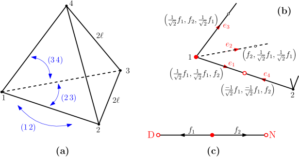
Figure 4.2. Tetrahedron quantum graph and its quotient construction via description of the intertwiner space.

The group $S_{4}$ of all permutations of the 4 vertices induces an action on $L^{2}(\Gamma)$ that leaves the domain of the operator invariant. For the purpose of quotient construction, we add “dummy” vertices at the midpoints of every edge. The conditions at the new vertices are Neumann-Kirchhoff, which preserves the domain of the operator modulo obvious isometries.

We compute the quotient graph with respect to the standard representation (3.17) of $S_{4}$, which we repeat here for convenience

$$\rho_{(1\,2)}=\begin{pmatrix}0&-1&0\\ -1&0&0\\ 0&0&1\end{pmatrix},\ \rho_{(2\,3)}=\begin{pmatrix}0&0&1\\ 0&1&0\\ 1&0&0\end{pmatrix},\ \rho_{(3\,4)}=\begin{pmatrix}0&1&0\\ 1&0&0\\ 0&0&1\end{pmatrix},\ \rho_{(2\,4)}=\begin{pmatrix}1&0&0\\ 0&0&1\\ 0&1&0\end{pmatrix}.$$

We will compute the quotient by both parametrizing the intertwiner space $\mathrm{Hom}_{G}(\textrm{V}_{\rho},\textrm{Dom}(T))$ and by following Definition 4.5.

Let $e_{1}$ denote the edge from the vertex $1$ to the midpoint of the (former) edge $(1,2)$, see Fig. 4.2(b) where the edge labels are shown in red. The orbit of this edge covers the whole graph and it is fixed by the permutation $(3\,4)$.

Denote the row of the intertwiner $\phi$ corresponding to $e_{1}$ by $\phi_{e_{1}}=(\phi_{1,1},\phi_{1,2},\phi_{1,3})$, where each $\phi_{1,j}$ belongs to $H^{2}(e_{1})=H^{2}([0,\ell/2])$. We first take care of the stabilizer group which imposes the condition

$$\phi_{e_{1}}=\phi_{e_{1}}\rho_{(3\,4)}.$$ (4.29)

We therefore parametrize $\phi_{e_{1}}$ as

$$\phi_{e_{1}}=\left(\frac{1}{\sqrt{2}}f_{1},\frac{1}{\sqrt{2}}f_{1},f_{2}\right),\qquad(f_{1},f_{2})\in H^{2}([0,\ell/2])\oplus H^{2}([0,\ell/2]),$$ (4.30)

where the factors $1/\sqrt{2}$ are added to make it a linear isometry (up to an overall factor). We fill out the other rows of $\phi$ as follows.

Since the edge $e_{1}$ is the image of $e_{2}$ under the action of $(2\,3)$, we have

$$\phi_{e_{2}}=\phi_{e_{1}}\rho_{(2\,3)}=\left(f_{2},\frac{1}{\sqrt{2}}f_{1},\frac{1}{\sqrt{2}}f_{1}\right).$$ (4.31)

Similarly, we get

$$\phi_{e_{3}}=\phi_{e_{2}}\rho_{(3\,4)}=\left(\frac{1}{\sqrt{2}}f_{1},f_{2},\frac{1}{\sqrt{2}}f_{1}\right),\quad\text{and}\quad\phi_{e_{4}}=\phi_{e_{1}}\rho_{(1\,2)}=\left(\frac{-1}{\sqrt{2}}f_{1},\frac{-1}{\sqrt{2}}f_{1},f_{2}\right).$$ (4.32)

This is enough to compute the matching conditions on the functions $f_{1},f_{2}\in H^{2}([0,\ell/2])$. From NK conditions at the vertex of degree 3 we have

$$\frac{1}{\sqrt{2}}f_{1}(0)=f_{2}(0)\quad\text{and}\quad\sqrt{2}f_{1}^{\prime}(0)+f_{2}^{\prime}(0)=0.$$ (4.33)

At the vertex of degree 2 (empty circle in Fig. 4.2(b)) we have

$$\frac{1}{\sqrt{2}}f_{1}(\ell/2)=\frac{-1}{\sqrt{2}}f_{1}(\ell/2),\quad -\frac{1}{\sqrt{2}}f_{1}^{\prime}(\ell/2)-\frac{-1}{\sqrt{2}}f_{1}^{\prime}(\ell/2)=0,$$

$$f_{2}(\ell/2)=f_{2}(\ell/2),\quad -f_{2}^{\prime}(\ell/2)-f_{2}^{\prime}(\ell/2)=0.$$

which are equivalent to

$$f_{1}(\ell/2)=0,\qquad f_{2}^{\prime}(\ell/2)=0.$$ (4.34)

To summarize, conditions (4.33) and (4.34) define a self-adjoint operator, acting as before by $-d^{2}/dx^{2}+q(x)$ on the edges of the graph in Fig. 4.2(c).

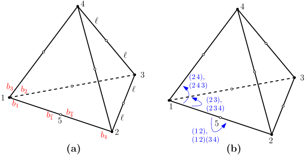
Figure 4.3. Tetrahedron quantum graph and the symmetry group action on the edge endpoints.

We now construct the quotient graph by following Definition 4.5. The symmetry group $S_{4}$ has an induced action on the edge endpoints, which we denote $b_{1},b_{2},\ldots,b_{\emph{$\overline{1}$}},b_{\emph{$\overline{2}$}},\ldots$, see Fig. 4.3(a). There are two orbits under the group action, and we choose $b_{1}$ and $b_{\emph{$\overline{1}$}}$ as the representatives.

The vertex conditions are local in that they only link the Dirichlet and Neumann values among the endpoints incident to the same vertex. We can therefore work locally, separately treating the block of $A$ (or $B$) corresponding to $\{b_{1},b_{2},b_{3}\}$ (incident to the vertex of degree 3) and the block of $A$ corresponding to $\{b_{\emph{$\overline{1}$}},b_{\emph{$\overline{4}$}}\}$ (incident to the midpoint vertex labeled by $5$ in Fig. 4.3).

After symmetrization (4.9), the corresponding blocks of $A$ and $B$ are

$$A=\frac{1}{3}\begin{pmatrix}2&-1&-1\\ -1&2&-1\\ -1&-1&2\end{pmatrix},\qquad B=\frac{1}{3i}\begin{pmatrix}1&1&1\\ 1&1&1\\ 1&1&1\end{pmatrix}$$ (4.35)

$$A=\frac{1}{2}\begin{pmatrix}1&-1\\ -1&1\end{pmatrix},\qquad B=\frac{1}{2i}\begin{pmatrix}1&1\\ 1&1\end{pmatrix}.$$ (4.36)

The stabilizer groups of $b_{1}$ and $b_{\emph{$\overline{1}$}}$ are $G_{b_{1}}=G_{b_{\emph{$\overline{1}$}}}=\{e,(3\,4)\}$ and therefore a valid choice of $\Phi$ is

$$\Phi_{b_{1}}=\Phi_{b_{\emph{$\overline{1}$}}}=\begin{pmatrix}\frac{1}{\sqrt{2}}&0\\ \frac{1}{\sqrt{2}}&0\\ 0&1\end{pmatrix}.$$ (4.37)

Due to locality of the vertex conditions, the summation in equation (4.14) can be restricted to the subgroups fixing vertex $1$ and the midpoint vertex $5$, correspondingly. For vertex $1$ the subgroup is $\{e,(3\,4),(2\,3),(2\,3\,4),(2\,4),(2\,4\,3)\}$. Using $(2\,3\,4)=(2\,3)(3\,4)$ and $(2\,4\,3)=(2\,4)(3\,4)$ to exploit the invariance properties of $\Phi_{b_{1}}$, we write

$$\left[A_{\rho}\right]_{b_{1},b_{1}} =\frac{1}{2}\Phi_{b_{1}}^{*}\Big{(}A_{b_{1},b_{1}}\big{(}e+(3\,4)\big{)}+A_{b_{1},b_{2}}(2\,3)\big{(}e+(3\,4)\big{)}+A_{b_{1},b_{3}}(2\,4)\big{(}e+(3\,4)\big{)}\Big{)}\Phi_{b_{1}}$$

$$=\Phi_{b_{1}}^{*}\big{(}A_{b_{1},b_{1}}e+A_{b_{1},b_{2}}(2\,3)+A_{b_{1},b_{3}}(2\,4)\big{)}\Phi_{b_{1}}=\frac{1}{3}\begin{pmatrix}1&-\sqrt{2}\\ -\sqrt{2}&2\end{pmatrix}.$$ (4.38)

Similarly for $B_{\rho}$,

$$\left[B_{\rho}\right]_{b_{1},b_{1}}=\frac{1}{3i}\begin{pmatrix}2&\sqrt{2}\\ \sqrt{2}&1\end{pmatrix}$$ (4.39)

These matrices are the symmetrized versions of the condition (4.33).

For the midpoint vertex $4$, the relevant subgroup is $\{e,(3\,4),(1\,2),(1,2)(3\,4)\}$ and the quotient vertex conditions are

$$\left[A_{\rho}\right]_{b_{\emph{$\overline{1}$}},b_{\emph{$\overline{1}$}}}=\Phi_{b_{\emph{$\overline{1}$}}}^{*}\big{(}A_{b_{\emph{$\overline{1}$}},b_{\emph{$\overline{1}$}}}e+A_{b_{\emph{$\overline{1}$}},b_{\emph{$\overline{4}$}}}(1\,2)\big{)}\Phi_{b_{\emph{$\overline{1}$}}}=\begin{pmatrix}1&0\\ 0&0\end{pmatrix},\quad\text{and}\quad\left[B_{\rho}\right]_{b_{\emph{$\overline{1}$}},b_{\emph{$\overline{1}$}}}=\frac{1}{i}\begin{pmatrix}0&0\\ 0&1\end{pmatrix},$$ (4.40)

in agreement with (4.34).

Example 4.11 (Tetrahedron revisited).

The quotient graph we computed in Example 4.10 does not cover all triply degenerate eigenvalues of the tetrahedron graph. This is because the group $S_{4}$, in addition to the standard representation $\rho$ given by (3.17) has another 3-dimensional representation. This representation is obtained by multiplying all matrices in equation (3.17) by $-1$ and we will denote it by $\hat{\rho}$.

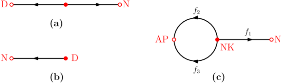
Figure 4.4. Various quotients of the tetrahedron quantum graph from Example 4.11.

The procedure for computing the quotient with respect to $\hat{\rho}$ is identical to the one followed in Example 4.10 with the only significant difference being in the matrix $\Phi$. The result is shown in Fig. 4.4(b); it is a single interval of length $\ell$ with Dirichlet and Neumann conditions.

In fact, the two quotients can be “joined” in a single graph, shown in Fig. 4.4(c). The conditions at the central vertex are the standard NK (as opposed to the more exotic conditions at the corresponding vertex of the quotient in Fig. 4.4(a)); the conditions at the left vertex are “anti-periodic”,

$$f_{2}(\ell)=-f_{3}(\ell),\qquad f_{2}^{\prime}(\ell)=f_{3}^{\prime}(\ell).$$ (4.41)

This graph has $C_{2}$ symmetry (up-down reflection) and the quotients with respect to this symmetry are exactly $\Gamma_{\rho}$ and $\Gamma_{\hat{\rho}}$ shown in Fig. 4.4(a) and (b).

The graph in Fig. 4.4(c) captures all triply degenerate eigenvalues of the tetrahedron graph $\Gamma$ for a typical potential. With the hindsight, we can get to this graph more directly, by restricting the representation $\rho$ to the subgroup $A_{4}$ of $S_{4}$ consisting of all even permutations. This restricted representation $\sigma$ is specified by

$$\sigma\colon(2\,3\,4)\mapsto\begin{pmatrix}0&0&1\\ 1&0&0\\ 0&1&0\end{pmatrix},\qquad(1\,2)(3\,4)\mapsto\begin{pmatrix}-1&0&0\\ 0&-1&0\\ 0&0&1\end{pmatrix},$$ (4.42)

and has the property that $\textrm{$\mathrm{Ind}$}_{A_{4}}^{S_{4}}\left(\sigma\right)=\rho\oplus\hat{\rho}$. Therefore, by Proposition 2.6, parts (3) and (1), the quotient $\Gamma_{\sigma}$ is unitarily equivalent to the direct sum of $\Gamma_{\rho}$ and $\Gamma_{\hat{\rho}}$. In fact, computing $\Gamma_{\sigma}$ is somewhat simpler because the stabilizer groups are trivial.

The same computation can be performed on the operator $H$ from Example 3.3, resulting in

$$H_{\sigma}=\begin{pmatrix}q_{\bullet}&a&a&a\\ a&q_{\circ}-b&0&0\\ a&0&q_{\circ}-b&0\\ a&0&0&q_{\circ}+b\end{pmatrix}.$$ (4.43)

The corresponding graph appears in Fig. 1.1(b).

5. Applications of Quotient Operators

In this section we point out some applications of quotient operators. In particular, we show how some earlier results are obtained as particular cases of the theory constructed in Section 2. This allows for extension of those earlier results and thus provides further applications.

5.1. Isospectrality

Proposition 2.6 may be perceived as an application of quotients to get isospectral examples. Indeed, that Proposition points out a few pairs of operators that are unitarily equivalent and hence isospectral. The third part of that Proposition allows to prove the following theorem which lies in the heart of many isospectral examples.

Theorem 5.1.

Let $G$ be a finite group. Let T be a finite dimensional operator which is $G$-symmetric. Let $H_{1},H_{2}$ be subgroups of $G$ with corresponding $H_{1}$-module $\textrm{V}_{\sigma_{1}}$ and $H_{2}$-module $\textrm{V}_{\sigma_{2}}$. If

$$\textrm{$\mathrm{Ind}$}_{H_{1}}^{G}\left(\textrm{V}_{\sigma_{1}}\right)\cong\textrm{$\mathrm{Ind}$}_{H_{2}}^{G}\left(\textrm{V}_{\sigma_{2}}\right),$$ (5.1)

then $\textrm{T}_{\sigma_{1}}$ and $\textrm{T}_{\sigma_{2}}$ are unitarily equivalent and, hence, isospectral.

Proof.

The proof is a straightforward corollary of Proposition 2.6,(3). Denote $\textrm{V}_{\rho_{n}}\cong\textrm{$\mathrm{Ind}$}_{H_{n}}^{G}\left(\textrm{V}_{\sigma_{n}}\right)$ for $n=1,2$. By (2.16) in Proposition 2.6 we get $\textrm{T}_{\sigma_{n}}\cong\textrm{T}_{\rho_{n}}$ for both $i=1,2$. The condition (5.1), or equivalently $\textrm{V}_{\rho_{1}}=\textrm{V}_{\rho_{2}}$ implies $\textrm{T}_{\rho_{1}}\cong\textrm{T}_{\rho_{2}}$ and finishes the proof. ∎

To connect this theorem to existing isospectral examples in the literature, we first refer to the pioneering work of Sunada [Sun85], which provided a general method for the construction of isospectral objects. That construction is based on taking the “trivial” quotients of a manifold by some groups in the following sense. Let $M$ be a manifold with a group $G$ acting on it. Let $H_{1}$ and $H_{2}$ be subgroups of $G$ which satisfy the following condition

$$\forall g\in G,\quad\quad~{}~{}~{}\left|\left[g\right]\cap H_{1}\right|=\left|\left[g\right]\cap H_{2}\right|,$$ (5.2)

where $\left[g\right]$ indicates the conjugacy class of $g$. In [Sun85, Thm. 1] it is stated that if condition (5.2) holds then the quotient manifolds $\nicefrac{{M}}{{H_{1}}}$, $\nicefrac{{M}}{{H_{2}}}$ are isospectral, . It is shown in [Bro99b, Pes94] that (5.2) is equivalent to the alternative condition

$$\textrm{$\mathrm{Ind}$}_{H_{1}}^{G}\left(\mathrm{V_{triv}}_{H_{1}}\right)\cong\textrm{$\mathrm{Ind}$}_{H_{2}}^{G}\left(\mathrm{V_{triv}}_{H_{2}}\right),$$ (5.3)

where $\mathrm{V_{triv}}_{H_{n}}$ is the trivial representation of $H_{n}$ ($n=1,2$).

Observe that the condition (5.3) in Sunada’s theorem is a particular case of condition (5.1) in Theorem 5.1 when $\sigma_{n}=\mathrm{triv}H_{n}$ for both $n=1,2$. In this case, the isospectrality implied by Theorem 5.1 is the same as Sunada’s, once it is shown that the topological quotient, $\nicefrac{{M}}{{H_{n}}}$, is the same manifold as the quotient $M_{\mathrm{triv}H_{n}}$. This indeed follows by the quotient definition in [BPBS09, PB10] and in that sense, [BPBS09, PB10] extended Sunada’s isospectrality theorem (Indeed see [BPBS09, Cor 4.4], [PB10, Cor 4] for the manifold and metric graph version of Theorem 5.1). Another aspect of [BPBS09, PB10] is the adjustment of the theory from manifolds to quantum (metric) graphs. In the current paper we provide the discrete graph analogue of this isospectral theory (which actually holds for any finite-dimensional operator). Moreover, in Section 4 we show that our methods extend to metric graphs (where the operator of interest is unbounded) and provide a more explicit and compact construction of a quotient quantum graph than the one given in [BPBS09, PB10].

In light of the above we are now able to re-examine some earlier works on isospectrality of discrete graphs and show how previous results may be obtained as particular applications of the theory in the current paper.

Regular graphs and free group action

In [Bro99a] Brooks considers $k$-regular graphs and groups which act freely on them and constructs isospectral graphs. Explicitly, Theorem 1.1 in [Bro99a] can be viewed as a particular case of Theorem 5.1 above, in the following sense: We take T in Theorem 5.1 to be the discrete Laplacian on some $k$-regular graph,

$$\textrm{T}_{i,j}=\begin{cases}1-\frac{1}{k}A_{i,i}&i=j\\ -\frac{1}{k}A_{i,j}&i\neq j\end{cases},$$ (5.4)

where $A_{i,j}$ indicates the number of edges connecting $i$ with $j$ (and in $A_{i,i}$ every loop is counted twice). Assume that T is $G$-symmetric and the group $G$ acts freely on the graph vertices. Take two subgroups $H_{1},H_{2}<G$, which satisfy condition (5.1) with their trivial representations $\sigma_{n}=\mathrm{triv}H_{n}$ ($n=1,2$). In order to express the operators $\textrm{T}_{\mathrm{triv}H_{1}}$ and $\textrm{T}_{\mathrm{triv}H_{2}}$ we may employ formulas (2.6) (thanks to using trivial representation) and (2.7) (thanks to the free actions) and have

$$\left[\textrm{T}_{\mathrm{triv}H_{n}}\right]_{i,j}=\sum_{g\in H_{n}}\textrm{T}_{i,gj}.$$ (5.5)

Both $\textrm{T}_{\mathrm{triv}H_{1}}$ and $\textrm{T}_{\mathrm{triv}H_{2}}$ are also normalized Laplacians corresponding to $k$-regular graphs. By Theorem 5.1 we get that they are isospectral and this is exactly the statement of Theorem 1.1 in [Bro99a].

Graph Laplacians and weak fixed point condition

Halbeisen and Hungerbühler extend in [HH99] the isospectral construction of Brooks. They consider graphs which are not necessarily $k$-regular and a group action which is not necessarily free. They consider the (non-normalized) Laplacian, $\textrm{T}=D-A$, where $A$ is the adjacency matrix (as in (5.4)) and $D$ is a diagonal matrix of vertex degrees. Assume that T is $G$-symmetric, and replace the free action requirement by a weaker condition, which in our terminology may be stated as $\left\{\textrm{T}_{i,j}\neq 0~{}\textrm{and }i,j\in\mathcal{D}\right\}~{}\Rightarrow~{}G_{i}=G_{j}$. Namely, if two vertices in the fundamental domain are adjacent then their stabilizers are equal. Employing this condition in our formula (2.6), we get $\left[\textrm{T}_{\mathrm{triv}G}\right]_{i,j}=\sum_{j^{\prime}\in O_{j}}\textrm{T}_{i,j^{\prime}}$. It can be checked that this quotient operator, $\textrm{T}_{\mathrm{triv}G}$, is exactly the (non-normalized) Laplacian associated with the quotient graph. In this case our quotient graph, $\Gamma_{\mathrm{triv}G}$, is identical to the quotient graph in the topological sense, $\nicefrac{{\Gamma}}{{G}}$. Using this construction, [HH99] in effect employ condition (5.1) with $\sigma_{1}=\mathrm{triv}H_{1}$, $\sigma_{2}=\mathrm{triv}H_{2}$ to generate examples of isospectral discrete graphs. We stated above their construction using our terminology, whereas in [HH99] it is done and proven differently.

Isospectral quantum (metric) graphs

We mentioned above that an isospectral construction for metric graphs in the spirit of the current paper already appeared in [BPBS09, PB10]. In Section 4 we provide an alternative construction of a quotient metric graphs which together with Proposition 2.6 and Theorem 5.1 may be used to provide isospectral examples of metric graphs. With this construction we may recover earlier isospectral examples such as the ones in [GS01, BSS06, BSS10]. Furthermore, there are quite a few very interesting recent works on isospectrality of metric graphs [Pis23, KM21, FCLP23, Mut21, JL21, CP20, MP23, LSBS21]; among which the papers [Mut21, JL21] are actually based on the quotient construction presented here (these papers cite an earlier version of the present work). A natural question is which of the isospectral examples in those recent works may be reproduced using the theory presented here. We leave the thorough examination of this question and comparison of those isospectral methods to future works. Here we briefly explain how some of the isospectral constructions in [FCLP23, KM21] can be deduced from the theory presented in the current paper.

The paper [FCLP23] presents a construction method of isospectral graphs (both discrete and metric and including magentic fields). The heart of the isospectral method lies in theorem 5.7 of that paper (see also (3.1) there). This theorem presents a spectral decomposition of a special type of graphs. The graphs there are constructed from a basic building block which is duplicated according to a certain partition of some number $r\in\mathbb{N}$. Specifically, the partition is denoted by $A=(a_{1},a_{2},\ldots,a_{s})$, where $r=\sum_{i=1}^{s}a_{i}$, and the corresponding graph is denoted there by $F_{A,V_{1}}$. In [FCLP23, thm 5.7] the spectrum of this graph is shown to be equal to a union of spectra of some other smaller graphs. This spectral decomposition depends only on $r$, $r-s$ and the building block graph. Hence, any other partition $A^{\prime}$ of $r$ with the same value of $s$ would yield an isospectral graph $F_{A^{\prime},V_{1}}$. It can be shown that the spectral decomposition of [FCLP23, Theorem 5.7] may be obtained directly from Proposition 2.8,(2). To give more details, the graph $F_{A,V_{1}}$ is symmetric under the group $C_{a_{1}}\times C_{a_{2}}\times\ldots\times C_{a_{s}}$, where $A=(a_{1},a_{2},\ldots,a_{s})$ is the given partition and $C_{n}$ is the cyclic group of order $n$. Apart from the trivial representation, the group $C_{n}$ has an $n-1$ irreducible representations given by the non-trivial $n$-roots of unity. Taking all quotients with respect to those representations as in Proposition 2.8,(2) gives a spectral decomposition of $F_{A,V_{1}}$, which is very close to the one in [FCLP23, thm 5.7]. To get exactly the spectral decomposition in [FCLP23, thm 5.7] we need just to notice that the quotient of $F_{A,V_{1}}$ with respect to the trivial representation of $C_{a_{1}}\times C_{a_{2}}\times\ldots\times C_{a_{s}}$ is a graph which is still symmetric, but under the symmetry group $C_{s}$. Further applying Proposition 2.8,(2) for that graph yields exactly the spectral decomposition in [FCLP23, thm 5.7].

Incidentally, the isospectral graphs presented in [KM21, Example 1] may be obtained from the above construction with partitions $A=(2,2)$ and $A^{\prime}=(1,3)$. However, we ought to emphasize that [KM21] contains further isospectral construction methods; it is not clear to us at this point whether those can be reproduced from the theory presented here.

5.2. Spectral computations and graph factorization

In this section we focus on using the decompositions given in Proposition 2.6,(2) and in its spectral counterpart, Proposition 2.8,(2), to facilitate the computation of spectra of large symmetric graphs (or any other domain).

Spectral decomposition for computations: Chung–Sternberg formula

Chung and Sternberg use the idea of a quotient operator (although they do not use this term) as a tool for spectral computations [CS92] (see also Section 7.5 in the book of Chung [Chu97]). Explicitly, they calculate the eigenvalues of the discrete Laplacian of large symmetric graphs.

The graphs considered in [CS92] are taken to be symmetric with respect to a transitive action of a group $G$ on their vertices. Namely, every vertex can be transformed to every other by some group element; equivalently, the fundamental domain has only one vertex. In this case, all vertices are of the same degree. Assign weights $\{q_{e}\}$ to the edges connected to some vertex (the transitive action makes the choice of the particular vertex irrelevant) and denote their sum by $Q=\sum q_{e}$. The operator studied in [CS92] is the weighted (discrete) Laplacian

$$\textrm{T}_{i,j}=\mathbb{\boldsymbol{I}}-\begin{cases}\nicefrac{{q_{e}}}{{Q}}&i\textrm{ is connected to }j~{}\textrm{by edge}~{}e\\ 0&i\textrm{ is not connected to }j\end{cases}.$$ (5.6)

Note that (5.4) is a particular case of (5.6), with $q_{e}=1$ for all edges. Assume that T is $G$-symmetric. Given an irreducible representation $\rho$, we may apply our formula (2.5) to get the explicit form of the quotient operator. We choose $i$ to be a representative vertex, so that $\mathcal{D}=\{i\}$ and in this case (2.5) reads

$$\textrm{T}_{\rho}=\frac{1}{|G_{i}|}\sum_{g\in G}\left(\Phi_{i}^{*}\,\rho(g)\,\Phi_{i}\right)\textrm{T}_{i,gi},$$ (5.7)

with all notations similar to those of Definition 2.2. Namely, $\Phi_{i}$ is an $r\times d_{i}$ matrix whose columns form an orthonormal basis for $(\textrm{V}_{\rho})^{G_{i}}$, the $G_{i}$-invariant subspace of $\textrm{V}_{\rho}$.

We note that (5.7) is precisely the expression in equation (11) of [CS92]. To see this, we provide the following dictionary translating from our formula (2.5) to [CS92, eq. (11)]:

• $\left|G_{i}\right|=\left|H\right|=\left|C_{e}\right|$

• $\textrm{V}_{\rho}\cong W$,  $(\textrm{V}_{\rho})^{G_{i}}\cong W^{H}$

• $g=a$, and $\Phi_{i}^{*}\,\rho(g)\,\Phi_{i}$ is “$a$ evaluated on $W^{H}$”.

To conclude, the quotient expression in [CS92, eq. (11)] may be viewed as an application of Definition 2.2 for the particular case of a discrete Laplacian with a transitive action on its vertex set. Chung and Sternberg combine this with a matrix decomposition such as the one in Proposition 2.6,(2) to present the eigenvalues of a large graph as the union of the eigenvalues of its quotients. We hope that the generalized theory provided in the current paper would aid in further enhancement of eigenvalue computations in the spirit of [CS92].

Graph factorizations

A similar method of graph factorization appears in the classical book of Cvetković, Doob and Sachs [CDS95, Ch. 5.2]. They discuss the restriction of an operator on a graph to a particular irreducible representation. However, the reduction is to a system of linear equations rather than providing an explicit expression for the quotient operator (such as (2.5)). The discussion in [CDS95] mentions the spectral point of view of such factorization (similarly to [Chu97, CS92]), but lacks the algebraic aspect such as Proposition 2.6.

Another useful concept appearing in that book is the one of graph divisors [CDS95, Ch. 4]. In the literature a graph divisor is also known by other names: an equitable partition, a coloration, a quotient graph or an orbigraph [Sch74, PS82, Bro99a, DGMdO⁺19]. Using our terminology, a graph divisor is the quotient of an operator with respect to the trivial representation of a symmetry group. That the spectrum of a divisor is contained in the spectrum of the original graph is widely known, appearing for example in the books [CDS95, Ch. 4], [CRS10, Ch. 3.9], [God93, Ch. 5], [GR01, Ch. 9.3]. It is mentioned in [CDS95, Ch. 4] that the spectrum of a graph may be decomposed as the union of spectra of its divisor and codivisor, but without providing a general and explicit formula for the codivisor (such as, for instance, our Proposition 2.6,(2)).

This divisor–codivisor decomposition is further developed in a series of recent works [BFW17, FSSW17, FSW19] in the special case of $G$ being a cyclic group. In this sense, those works contain results which are particular cases of Proposition 2.6,(2).

Spectral decompositions on finite and infinite quantum (metric) graphs

Spectral decompositions for metric graphs in the form of Proposition 2.8 are used for various purposes in spectral analysis. For instance, [Exn21, EL19] studied the spectra of graphs formed by the edges of platonic solids. Naturally, these graphs are symmetric with respect to well-known groups. Hence, spectral computations in [Exn21, EL19] (which cite an earlier version of the present work) are made mush easier by a decomposition of the type established in Proposition 2.8.

A decomposition of the Laplacian on radially symmetric metric trees by Naimark–Solomyak [NS01, Sol04] was very influential in the modern spectral theory of non-compact metric graphs. More recently, in the series of works [BK13b, BK22, BL20, KN21], the decomposition of Naimark–Solomyak was extended to metric and discrete non-compact graphs with partial spherical symmetry.

We expect that this decomposition can also be understood in the spirit of Proposition 2.8,(2), but for non-compact metric graphs and infinite symmetry groups (which are infinite products of finite groups). The works [BK13b, BK22, BL20] do not explicitly describe the symmetry groups of the underlying graphs and there is still work to be done to link the two approaches.

Finally, we mention that the results presented here were used to significantly simplify computations of the spectrum of a Euler–Bernoulli beam structure in [BE22]. The model therein is a fourth order differential operator acting on vector-valued functions supported on a symmetric graph. While the graph and its symmetry groups are simple, the high order of the operator makes analysis without spectral decomposition prohibitively cumbersome.

Appendix A A primer on representation theory

We bring here the relevant definitions and statements from representation theory of finite groups. In particular, we make the connection between group module terminology to matrix representation terminology. We are aware that there are many who are not familiar with the former, but are very fond of the latter.

A.1. Representations and $G$-modules

Definition A.1.

Let $G$ be a finite group. Let $V$ be a vector space over $\mathbb{C}$.

1. A group homomorphism, $\rho:G\rightarrow\textrm{GL}(V)$ is called a representation of $G$.

2. The group algebra $\mathbb{C}G$ consists of the elements $\sum_{g\in G}c_{g}g$ with $c_{g}\in\mathbb{C}$, and multiplication in $\mathbb{C}G$ extends the multiplication in $G$.
   We say that $V$ is a (left) $\mathbb{C}G$-module (or $G$-module) if there is an action of $\mathbb{C}G$ on $V$ (i.e., a map $\mathbb{C}G\times V\rightarrow V$) denoted by $r\cdot v$ for all $r\in\mathbb{C}G$, $v\in V$, such that the following holds:

   1. $(r+s)\cdot v=r\cdot v+s\cdot v$ for all $r,s\in\mathbb{C}G$, $v\in V$.

   2. $(rs)\cdot v=r\cdot(s\cdot v)$ for all $r,s\in\mathbb{C}G$, $v\in V$.

   3. $r\cdot(v+u)=r\cdot v+r\cdot u$ for all $r\in\mathbb{C}G$, $v,u\in V$.

   4. $1\cdot v=v$ for all $v\in V$, where $1\in G$ is the identity element.

Remark A.2.

We will call $V$ as in Definition A.1,(2) a $G$-module rather than a $\mathbb{C}G$-module. Both terms are interchangeably used in the literature (see [FH13, DF04]).

The two parts of Definition A.1 are the same. Namely, if $\rho:G\rightarrow\textrm{GL}(V)$ is a representation of $G$, then $V$ becomes a $G$-module by

$$\forall v\in V,\quad\left(\sum_{g\in G}c_{g}g\right)\cdot v=\sum_{g\in G}c_{g}\thinspace\rho(g)\thinspace v.$$

Conversely, if $V$ is a $G$-module, then $\rho:G\rightarrow\textrm{GL}(V)$ defined by $\rho(g)\thinspace v=g\cdot v$ is a representation. See more in [Bum13, sec. 34].

In light of the above, we tend to denote $\textrm{V}_{\rho}$ to emphasize the connection between the module and the corresponding representation.

To develop and prove the theory in this paper it is more convenient to use the module terminology rather than the matrix representation one. On the other hand, working out the examples requires the use of specific matrix representations. Hence, both approaches are mentioned throughout the paper.

A.2. Intertwiners

Let $G$ be a finite group and $\textrm{V}_{\rho}$ and $\textrm{V}_{\pi}$ be two $G$-modules. Denote by $\mathrm{Hom}(\textrm{V}_{\rho},\textrm{V}_{\pi})\cong\textrm{V}_{\rho}^{*}\otimes\textrm{V}_{\pi}$ the space of linear homomorphisms between the vector spaces $\textrm{V}_{\pi}$ and $\textrm{V}_{\rho}$. We consider $\mathrm{Hom}(\textrm{V}_{\rho},\textrm{V}_{\pi})$ as a $G$-module, with the following action, $g\times\phi\mapsto g\phi g^{-1}$ for all $g\in G$ and $\phi\in\mathrm{Hom}(\textrm{V}_{\rho},\textrm{V}_{\pi})$. The set of fixed points of this action is denoted by

$$\mathrm{Hom}_{G}(\textrm{V}_{\rho},\textrm{V}_{\pi}):=\left\{\phi\in\mathrm{Hom}(\textrm{V}_{\rho},\textrm{V}_{\pi})~{}:~{}g\phi=\phi g\right\}.$$ (A.1)

This is a linear space, known as the trivial isotypic component of $\mathrm{Hom}(\textrm{V}_{\rho},\textrm{V}_{\pi})$ and it is also common to refer to the elements $\phi\in\mathrm{Hom}_{G}(\textrm{V}_{\rho},\textrm{V}_{\pi})$ as intertwiners.

In this paper we consider only finite dimensional $G$-modules and assume that they are equipped with an inner product (hence, they are Hilbert spaces). We also define the following inner product on the space of intertwiners,

$$\left\langle\phi_{1},\phi_{2}\right\rangle_{\mathrm{Hom}_{G}(\textrm{V}_{\rho},\textrm{V}_{\pi})}:=\textrm{Tr}\left(\phi_{2}^{*}\phi_{1}\right)=\sum_{v\in B(\textrm{V}_{\rho})}\left\langle\phi_{1}(v)\thinspace,\thinspace\phi_{2}(v)\right\rangle_{\textrm{V}_{\pi}},$$ (A.2)

where $\left\langle\phantom{}~{},~{}\phantom{}\right\rangle_{\textrm{V}_{\pi}}$ denotes the inner product in $\textrm{V}_{\pi}$ and $B(\textrm{V}_{\rho})$ is some choice of basis for $\textrm{V}_{\rho}$ (obviously, it can be shown that the inner product above does not depend on the choice of basis). This is just the usual Frobenius inner product on the space of finite dimensional linear operators, restricted to $\mathrm{Hom}_{G}(\textrm{V}_{\rho},\textrm{V}_{\pi})$.

A.3. Induced representations and Frobenius reciprocity

There is more than one standard way to present induced representations and Frobenius reciprocity. Here we follow the one in [Bum13, sec. 34], which suits the needed arguments for the proofs in Section 2.

Definition A.3.

Let $H$ be a subgroup of a finite group $G$. Let $\textrm{V}_{\sigma}$ be an $H$-module. Define the induced representation (from $H$ to $G$), $\textrm{V}_{\rho}:=\textrm{$\mathrm{Ind}$}_{H}^{G}\left(\textrm{V}_{\sigma}\right)$, as the following $G$-module,

$$\textrm{V}_{\rho}=\left\{f:G\rightarrow\textrm{V}_{\sigma}~{}:~{}f(hg)=\sigma(h)f(g),~{}~{}\forall h\in H\right\},$$ (A.3)

where the $G$ action is by $\left(\rho(g)f\right)(\tilde{g}):=f(\tilde{g}g)$ for all $f\in\textrm{V}_{\rho}$ and $g,\tilde{g}\in G$.

On the induced representation, $\textrm{$\mathrm{Ind}$}_{H}^{G}\left(\textrm{V}_{\sigma}\right)$, we fix the following inner product:

$$\forall f_{1},f_{2}\in\textrm{$\mathrm{Ind}$}_{H}^{G}\left(\textrm{V}_{\sigma}\right),\quad\quad\left\langle f_{1},f_{2}\right\rangle:=\frac{1}{\left|G\right|}\sum_{g\in G}\left\langle f_{1}(g)\thinspace,\thinspace f_{2}(g)\right\rangle_{\textrm{V}_{\sigma}}.$$ (A.4)

As a straightforward exercise, the reader might compute that when taking $H=\{\mathrm{id}\}$ (the trivial group) and $\textrm{V}_{\sigma}$ to be the trivial representation of $H$, we obtain in the definition above $\textrm{V}_{\rho}=\mathbb{C}G$ and so $\textrm{$\mathrm{Ind}$}_{H}^{G}\left(\textrm{V}_{\sigma}\right)=\textrm{reg}_{G}$, where $\textrm{reg}_{g}$ is the regular representation of $G$. This observation is used in the proof of Proposition 2.6,(2).

Theorem A.4.

[Frobenius reciprocity Theorem] [Bum13, sec. 34]

Let $H$ be a subgroup of a finite group $G$. Let $\textrm{V}_{\sigma}$ be an $H$-module and $\textrm{V}_{\pi}$ be a $G$-module. Then

1. $\mathrm{Hom}_{H}\left(\textrm{V}_{\pi},\textrm{V}_{\sigma}\right)$ is isomorphic to $\mathrm{Hom}_{G}\left(\textrm{V}_{\pi},\textrm{$\mathrm{Ind}$}_{H}^{G}\left(\textrm{V}_{\sigma}\right)\right)$.
   This isomorphism maps $\phi\in\mathrm{Hom}_{H}\left(\textrm{V}_{\pi},\textrm{V}_{\sigma}\right)$ to $\Phi\in\mathrm{Hom}_{G}\left(\textrm{V}_{\pi},\textrm{$\mathrm{Ind}$}_{H}^{G}\left(\textrm{V}_{\sigma}\right)\right)$ defined by

   $$\Phi(v)(g)=\phi(\pi(g)v).$$ (A.5)

   for $v\in\textrm{V}_{\pi}$ and $g\in G$.

2. $\mathrm{Hom}_{H}\left(\textrm{V}_{\sigma},\textrm{V}_{\pi}\right)$ is isomorphic to $\mathrm{Hom}_{G}\left(\textrm{$\mathrm{Ind}$}_{H}^{G}\left(\textrm{V}_{\sigma}\right),\textrm{V}_{\pi}\right)$.
   This isomorphism maps $\phi\in\mathrm{Hom}_{H}\left(\textrm{V}_{\sigma},\textrm{V}_{\pi}\right)$ to $\Phi\in\mathrm{Hom}_{G}\left(\textrm{$\mathrm{Ind}$}_{H}^{G}\left(\textrm{V}_{\sigma}\right),\textrm{V}_{\pi}\right)$ defined by

   $$\Phi:\textrm{$\mathrm{Ind}$}_{H}^{G}\left(\textrm{V}_{\sigma}\right)\to\textrm{V}_{\pi},\qquad\Phi:f\mapsto\frac{\left|H\right|}{\left|G\right|}\sum_{g\in G/H}\pi(g)\thinspace\phi(f(g^{-1})),$$ (A.6)

   where the sum is over some choice of representatives of $H$ left cosets in $G$ (and does not depend on the particular choice of the representatives).

Remark.

For any two $G$-modules, $\textrm{V}_{\sigma},\textrm{V}_{\pi}$ it is not hard to see that $\mathrm{Hom}_{H}\left(\textrm{V}_{\pi},\textrm{V}_{\sigma}\right)\cong\mathrm{Hom}_{H}\left(\textrm{V}_{\sigma},\textrm{V}_{\pi}\right)$, where the isomorphism is explicitly given by the adjoint. Hence, the two parts of the theorem above are equivalent in the sense of existence of isomorphisms. Yet, we bring both versions (as in [Bum13, sec. 34]) since the explicit form of the isomorphisms is useful for the proofs in the paper. The first part of the theorem is used in proving Theorem 2.5 and the second is used in the proof of Proposition 2.6,(3).

Remark.

In (A.6) above we have introduced a prefactor as part of Frobenius maps which does not appear in [Bum13, sec. 34]. Obviously, such a factor does not affect the map being an isomorphism, but it is used to show that the map is unitary.

In the current paper we need to use that the Frobenius reciprocity is not only an isomorphism, but that it also preserves the inner product. As we did not find explicit references to this observation, we complement Theorem A.4 by stating and proving this.

Proposition A.5.

Both isomorphisms in Theorem A.4 preserve the inner product.

Remark A.6.

The following proof may be simplified by observing that the two Frobenius isomorphisms are adjoints of each other and checking unitarity for only one of them.

Proof.

We first show that the isomorphism in Theorem A.4,(1) preserves the inner product.

Let $\phi_{1},\phi_{2}\in\mathrm{Hom}_{H}(\textrm{V}_{\pi},\textrm{V}_{\sigma})$ and $\Phi_{1},\Phi_{2}\in\mathrm{Hom}_{G}\left(\textrm{V}_{\pi},\textrm{$\mathrm{Ind}$}_{H}^{G}\left(\textrm{V}_{\sigma}\right)\right)$ the corresponding images by the Frobenius reciprocity map (A.5).

$$\left\langle\Phi_{1}~{},~{}\Phi_{2}\right\rangle_{\mathrm{Hom}_{G}\left(\textrm{V}_{\pi},\textrm{$\mathrm{Ind}$}_{H}^{G}\left(\textrm{V}_{\sigma}\right)\right)} =\sum_{v\in B(\textrm{V}_{\pi})}\left\langle\Phi_{1}(v)~{},~{}\Phi_{2}(v)\right\rangle_{\textrm{$\mathrm{Ind}$}_{H}^{G}\left(\textrm{V}_{\sigma}\right)}$$

$$=\frac{1}{\left|G\right|}\sum_{v\in B(\textrm{V}_{\pi})}\sum_{g\in G}\left\langle\Phi_{1}(v)(g)~{},~{}\Phi_{2}(v)(g)\right\rangle_{\textrm{V}_{\sigma}}$$

$$=\frac{1}{\left|G\right|}\sum_{v\in B(\textrm{V}_{\pi})}\sum_{g\in G}\left\langle\phi_{1}(\pi(g)v)~{},~{}\phi_{2}(\pi(g)v)\right\rangle_{\textrm{V}_{\sigma}}$$

$$=\frac{1}{\left|G\right|}\sum_{g\in G}\sum_{v\in B(\textrm{V}_{\pi})}\left\langle\phi_{1}(\pi(g)v)~{},~{}\phi_{2}(\pi(g)v)\right\rangle_{\textrm{V}_{\sigma}}$$

$$=\frac{1}{\left|G\right|}\sum_{g\in G}\left\langle\phi_{1}~{},~{}\phi_{2}\right\rangle_{\mathrm{Hom}_{H}(\textrm{V}_{\pi},\textrm{V}_{\sigma})}=\left\langle\phi_{1}~{},~{}\phi_{2}\right\rangle_{\mathrm{Hom}_{H}(\textrm{V}_{\pi},\textrm{V}_{\sigma})}$$

where moving to the last line we used the fact that for any $g\in G$, the set $\left\{\pi(g)\thinspace v\right\}_{v\in B(\textrm{V}_{\pi})}$ is a basis for $\textrm{V}_{\pi}$.

Next, we show that the isomorphism in Theorem A.4,(2) preserves the inner product.

We define for each $g\in G$ and $v\in\textrm{V}_{\sigma}$ the following map

$$\epsilon_{g}(v) :G\rightarrow\textrm{V}_{\sigma}$$

$$\epsilon_{g}(v) (\tilde{g})=\sqrt{\nicefrac{{\left|G\right|}}{{\left|H\right|}}}\begin{cases}\sigma(\tilde{g}g)v&\textrm{if}~{}\tilde{g}g\in H,\\ 0&\textrm{otherwise}.\end{cases}$$

One can check that for all $g\in G$ and $v\in\textrm{V}_{\sigma}$, $\epsilon_{g}(v)\in\textrm{$\mathrm{Ind}$}_{H}^{G}\left(\textrm{V}_{\sigma}\right)$. We use the map $\epsilon_{g}(v)$ to construct a basis for $\textrm{$\mathrm{Ind}$}_{H}^{G}\left(\textrm{V}_{\sigma}\right)$ from a given basis for $\textrm{V}_{\sigma}$. Let $\left\{v_{i}\right\}$ some choice of an orthonormal basis for $\textrm{V}_{\sigma}$ and $\left\{g_{j}\right\}$ some choice of representatives for the right cosets of $H$. Then, it is straightforward to check that $\left\{\epsilon_{g_{j}}(v_{i})\right\}$ is an orthonormal basis for $\textrm{$\mathrm{Ind}$}_{H}^{G}\left(\textrm{V}_{\sigma}\right)$ (with the inner product (A.4)). Take $\phi\in\mathrm{Hom}_{H}(\textrm{V}_{\sigma},\textrm{V}_{\pi})$ which is sent by the Frobenius isomorphism to $\Phi\in\mathrm{Hom}_{G}(\textrm{$\mathrm{Ind}$}_{H}^{G}\left(\textrm{V}_{\sigma}\right),\textrm{V}_{\pi})$. This map is given explicitly in (A.6), so that

$$\forall i,j,\quad\quad\Phi(\epsilon_{g_{j}}(v_{i})) =\nicefrac{{\left|H\right|}}{{\left|G\right|}}\thinspace\sum_{g\in G/H}\pi(g)\thinspace\phi(\epsilon_{g_{j}}(v_{i})(g^{-1}))$$

$$=\sqrt{\nicefrac{{\left|H\right|}}{{\left|G\right|}}}\thinspace\pi(\tilde{g})\thinspace\phi(\sigma(\tilde{g}^{-1}g_{j})v_{i})$$

$$=\sqrt{\nicefrac{{\left|H\right|}}{{\left|G\right|}}}\thinspace\pi(g_{j})\thinspace\phi(v_{i}),$$ (A.7)

where in the second line we take $\tilde{g}\in G/H$ to be the $H$ left coset representative such that $g_{j}\in\tilde{g}H$, and on the third line we used that $\phi$ is an intertwiner. Applying (A.7), we show that the Frobenius isomorphism preserves the inner product. Indeed, take $\phi_{1},\phi_{2}\in\mathrm{Hom}_{H}(\textrm{V}_{\sigma},\textrm{V}_{\pi})$ which are sent by the Frobenius isomorphism to $\Phi_{1},\Phi_{2}\in\mathrm{Hom}_{G}(\textrm{$\mathrm{Ind}$}_{H}^{G}\left(\textrm{V}_{\sigma}\right),\textrm{V}_{\pi})$, correspondingly, and get

$$\left\langle\Phi_{1},\Phi_{2}\right\rangle =\sum_{i,j}\left\langle\Phi_{1}(\epsilon_{g_{j}}(v_{i}))\thinspace,\thinspace\Phi_{2}(\epsilon_{g_{j}}(v_{i}))\right\rangle_{\textrm{V}_{\pi}}$$

$$=\frac{\left|H\right|}{\left|G\right|}\sum_{i,j}\left\langle\pi(g_{j})\thinspace\phi_{1}(v_{i})\thinspace,\thinspace\pi(g_{j})\thinspace\phi_{2}(v_{i})\right\rangle_{\textrm{V}_{\pi}}$$

$$=\sum_{i}\left\langle\phi_{1}(v_{i})\thinspace,\thinspace\phi_{2}(v_{i})\right\rangle_{\textrm{V}_{\pi}}$$

$$=\left\langle\phi_{1},\phi_{2}\right\rangle,$$

where on the second line we used the unitarity of the representation $\pi$. ∎

Proposition A.7.

If $T:\textrm{V}_{\pi}\to\textrm{V}_{\pi}$ is a $G$-symmetric operator (as in Definition 2.1), then in commutes with the Frobenius isomorphism from $\mathrm{Hom}_{H}\left(\textrm{V}_{\sigma},\textrm{V}_{\pi}\right)$ to $\mathrm{Hom}_{G}\left(\textrm{$\mathrm{Ind}$}_{H}^{G}\left(\textrm{V}_{\sigma}\right),\textrm{V}_{\pi}\right)$ given by (A.6).

Proof.

For all $f\in\textrm{$\mathrm{Ind}$}_{H}^{G}\left(\textrm{V}_{\sigma}\right)$ we check

$$\textrm{T}\left[\sum_{g\in G/H}\pi(g)\thinspace\phi(f(g^{-1}))\right]=\sum_{g\in G/H}\textrm{T}\left[\pi(g)\thinspace\phi(f(g^{-1}))\right]=\sum_{g\in G/H}\pi(g)\thinspace\textrm{T}\left[\phi(f(g^{-1}))\right]\\ =\sum_{g\in G/H}\pi(g)\thinspace\textrm{T}\left[\phi\right](f(g^{-1})),$$

where the first equality follows by linearity, the second holds since T is $G$-symmetric and the last is the definition of T action on $\mathrm{Hom}_{H}(\textrm{V}_{\sigma},\textrm{V}_{\pi})$, see (2.11). To summarize, we get that $T\Phi$ is the element of $\mathrm{Hom}_{G}\left(\textrm{$\mathrm{Ind}$}_{H}^{G}\left(\textrm{V}_{\sigma}\right),\textrm{V}_{\pi}\right)$ corresponding to $T\phi\in\mathrm{Hom}_{H}\left(\textrm{V}_{\sigma},\textrm{V}_{\pi}\right)$ by the isomorphism (A.6). ∎

Appendix B Proofs of the properties of the quantum graph quotient

B.1. Preliminaries

The vectorization map is a linear transformation which converts a matrix to a column vector by essentially ‘stacking’ the columns on the matrix on top of each other. More formally

Definition B.1.

Let $A$ be an $m\times n$ matrix with $m$-dimensional column vectors $a_{1},\ldots,a_{n}$ then $\textrm{vec}{~{}}{:}~{}M_{m\times n}(\mathbb{C})\to\mathbb{C}^{nm}$ is the following map

$$\mathrm{vec}(A)=\mathrm{vec}((a_{1}\ldots a_{n}))=\begin{pmatrix}a_{1}\\ \vdots\\ a_{n}\end{pmatrix}=\sum_{i=1}^{n}(\mathbf{e}_{i}\otimes a_{i}),$$

which we call vectorization.

So, for example, if $\phi=(\phi_{1},\phi_{2})$ is the $2\times 2$ matrix, then

$$\phi_{1}=\begin{pmatrix}x_{1}\\ y_{1}\end{pmatrix},\quad\phi_{2}=\begin{pmatrix}x_{2}\\ y_{2}\end{pmatrix},\quad\Longrightarrow\mathrm{vec}(\phi)=\begin{pmatrix}x_{1}\\ y_{1}\\ x_{2}\\ y_{2}\end{pmatrix}.$$

Using the definition of $\mathrm{vec}$ we have the following trivial property for products of matrices.

Lemma B.2.

Let $A$ and $B$ be two $k\times n$ and $n\times m$ matrices respectively. Then

$$\mathrm{vec}(AB)=(\mathbb{\boldsymbol{I}}_{m}\otimes A)\thinspace\mathrm{vec}(B)=(B^{T}\otimes\mathbb{\boldsymbol{I}}_{k})\thinspace\mathrm{vec}(A).$$ (B.1)

Next, we define the matrix $\Theta$ whose columns are the orthonormal basis $\bigcup_{i\in\mathcal{D}}\left\{\theta_{i}^{(n)}\right\}_{n=1}^{d_{i}}$ for $\mathrm{Hom}_{G}(\textrm{V}_{\rho},\textrm{V}_{\pi})$, as given in Lemma 2.9.

Definition B.3.

Following the notation in Section 4.3, we denote for each $i\in\mathcal{D}$ and $1\leq i\leq d_{i}$, the map $\theta_{i}^{(n)}:\textrm{V}_{\rho}\rightarrow\textrm{V}_{\pi}$ by

$$\forall v\in\textrm{V}_{\rho},\quad\quad\theta_{i}^{(n)}(v):=\frac{1}{\sqrt{\left|G\right|\left|G_{i}\right|}}\sum_{g\in G}\left\langle\rho(g)\varphi_{i}^{(n)}\thinspace,\thinspace v\right\rangle_{\textrm{V}_{\rho}}\thinspace\mathbf{e}_{g\thinspace i},$$ (B.2)

exactly as in Lemma 2.9. With $r:=\dim\textrm{V}_{\rho}$ and $\dim\textrm{V}_{\pi}=\left|\mathcal{E}\right|$, consider each $\theta_{i}^{(n)}$ as an $\left|\mathcal{E}\right|\times r$ matrix, so that $\textrm{vec}{(}\theta_{i}^{(n)})$ is a column vector of length $\left|\mathcal{E}\right|r$.
Specifically, we define

$$\Theta_{i}=\frac{1}{\sqrt{\left|G\right|\left|G_{i}\right|}}\sum_{g\in G}\left(\overline{\rho(g)}\otimes\pi(g)\right)\left(\Phi_{i}\otimes\mathbf{e}_{i}\right),$$ (B.3)

to be a $\left|\mathcal{E}\right|r\times d_{i}$ matrix whose columns are $\left\{\textrm{vec}{(}\theta_{i}^{(n)})\right\}_{n=1}^{d_{i}}$. Subsequently, define $\Theta\in M_{\left|\mathcal{E}\right|r\times d}(\mathbb{C})$ to be

$$\Theta=\begin{pmatrix}\Theta_{1}&\Theta_{2}&\ldots&\Theta_{\left|\mathcal{D}\right|}\end{pmatrix}.$$ (B.4)

We also denote $\hat{\Theta}:=\Theta\otimes\mathbb{\boldsymbol{I}}_{2}$ (similarly to the $\hat{\pi}$ notation introduced in (4.10)),

Lemma B.4.

The matrices $\Theta\in M_{\left|\mathcal{E}\right|r\times d}(\mathbb{C})$ and $\hat{\Theta}\in M_{2\left|\mathcal{E}\right|r\times 2d}(\mathbb{C})$ defined above satisfy

1. $\Theta^{*}\Theta=\mathbb{\boldsymbol{I}}_{d}$ .

2. $\Theta\Theta^{*}=\frac{1}{|G|}\sum_{g\in G}\emph{$\overline{\rho(g)}$}\otimes\pi(g)$.

3. $\hat{\Theta}\hat{\Theta}^{*}$ commutes with $\mathbb{\boldsymbol{I}}_{r}\otimes A$ and $\mathbb{\boldsymbol{I}}_{r}\otimes B$.

4. $A_{\rho}=\hat{\Theta}^{*}[\mathbb{\boldsymbol{I}}_{r}\otimes A]\hat{\Theta}$ and $B_{\rho}=\hat{\Theta}^{*}[\mathbb{\boldsymbol{I}}_{r}\otimes B]\hat{\Theta}$.

5. $[\mathbb{\boldsymbol{I}}_{r}\otimes\pi(g)-\rho(g)^{T}\otimes\mathbb{\boldsymbol{I}}_{p}]\Theta=0$ for all $g\in G$.

Proof.

The proof of the first two parts of the Lemma are based on Lemma 2.9. In Lemma 2.9 it is stated that the maps $\theta_{i}^{(n)}:\textrm{V}_{\rho}\rightarrow\textrm{V}_{\pi}$ as defined in (B.2) form an orthonormal basis for $\mathrm{Hom}_{G}(\textrm{V}_{\rho},\textrm{V}_{\pi})$. Turning those maps to matrices and applying vec do not affect this quality. Hence we get that the columns of $\Theta$ form an orthonormal basis for $\mathrm{Hom}_{G}(\textrm{V}_{\rho},\textrm{V}_{\pi})$.

1. The orthonormality of $\Theta$ columns yields $\Theta^{*}\Theta=\mathbb{\boldsymbol{I}}_{2d}$, as in the first part of the Lemma.

2. That the columns form an orthogonal basis for $\mathrm{Hom}_{G}(\textrm{V}_{\rho},\textrm{V}_{\pi})$ implies that $\Theta\Theta^{*}$ is a projector from $\textrm{V}_{\rho}\otimes\textrm{V}_{\pi}=\mathrm{Hom}(\textrm{V}_{\rho},\textrm{V}_{\pi})$ onto $\mathrm{Hom}_{G}(\textrm{V}_{\rho},\textrm{V}_{\pi})$. To get the explicit expression of this projector, we note (see, for example, [FH13, Ch. 2.2]) that if $R$ is a unitary representation of $G$ on $V$ then the operator

   $$\mathbf{P}:=\frac{1}{|G|}\sum_{g\in G}R(g)$$

   is an orthogonal projector onto the trivial component of $R$, i.e.

   $$\textrm{Image}[\mathbf{P}]=\{v\in V_{R}~{}:~{}R(g)v=v~{}\quad\forall g\in G\}.$$

   Taking $R=\emph{$\overline{\rho}$}\otimes\pi$, where $\overline{\rho}$ is the dual representation of $\rho$ (see also [FH13, Ch. 1.1]), we get that $\frac{1}{|G|}\sum_{g\in G}\emph{$\overline{\rho(g)}$}\otimes\pi(g)$ is an orthogonal projector onto the trivial component of $\textrm{V}_{\rho}\otimes\textrm{V}_{\pi}=\mathrm{Hom}(\textrm{V}_{\rho},\textrm{V}_{\pi})$ which is $\mathrm{Hom}_{G}(\textrm{V}_{\rho},\textrm{V}_{\pi})$ (see [FH13, Ex. 1.2]). Therefore, $\Theta\Theta^{*}=\frac{1}{|G|}\sum_{g\in G}\emph{$\overline{\rho(g)}$}\otimes\pi(g)$, as in the second part of the Lemma.

We continue to prove the last three parts of the Lemma.

[resume]

1. Using the second part of the Lemma we get that

   $$\hat{\Theta}\hat{\Theta}^{*}=\frac{1}{|G|}\sum_{g\in G}\emph{$\overline{\rho(g)}$}\otimes\hat{\pi}(g).$$ (B.5)

   This clearly commutes with the matrices $\mathbb{\boldsymbol{I}}_{r}\otimes A$ and $\mathbb{\boldsymbol{I}}_{r}\otimes B$ because $A$ and $B$ commute with $\hat{\pi}(g)$ (as is assumed throughout the section and see also Lemma 4.3).

2. The assertions $A_{\rho}=\hat{\Theta}^{*}[\mathbb{\boldsymbol{I}}_{r}\otimes A]\hat{\Theta}$ and $B_{\rho}=\hat{\Theta}^{*}[\mathbb{\boldsymbol{I}}_{r}\otimes B]\hat{\Theta}$ are obtained as a corollary of Theorem 2.5, with the slight modification of considering $\hat{\pi}$ instead of $\pi$. To see this, we first observe that $\left.A\right|_{\mathrm{Hom}_{G}(\textrm{V}_{\rho},\mathrm{V}_{\hat{\pi}})}=\hat{\Theta}^{*}[\mathbb{\boldsymbol{I}}_{r}\otimes A]\hat{\Theta}$. This last observation follows from the linear action of $A$ on $\mathrm{Hom}_{G}(\textrm{V}_{\rho},\mathrm{V}_{\hat{\pi}})$ (see (2.11),(2.12)), when keeping in mind that the columns of $\hat{\Theta}$ forming an orthonormal basis for $\mathrm{Hom}_{G}(\textrm{V}_{\rho},\mathrm{V}_{\hat{\pi}})$ (as in the first two parts of this lemma). Now, Theorem 2.5 implies $A_{\rho}=\hat{\Theta}^{*}[\mathbb{\boldsymbol{I}}_{r}\otimes A]\hat{\Theta}$ when taking T to be $A$ and $\textrm{V}_{\pi}$ to be $\mathrm{V}_{\hat{\pi}}$. Exactly the same holds for $B$ and $B_{\rho}$.

3. Let $g\in G$. We show that $[\mathbb{\boldsymbol{I}}_{r}\otimes\pi(g)-\rho(g)^{T}\otimes\mathbb{\boldsymbol{I}}_{p}]\Theta\Theta^{*}=0$, which after right multiplication by $\Theta$ and applying the first part of the Lemma gives the needed statement.

   $$[\mathbb{\boldsymbol{I}}_{r}\otimes\pi(g)-\rho(g)^{T}\otimes\mathbb{\boldsymbol{I}}_{p}]\Theta\Theta^{*} =\frac{1}{|G|}[\mathbb{\boldsymbol{I}}_{r}\otimes\pi(g)-\rho(g)^{T}\otimes\mathbb{\boldsymbol{I}}_{p}]\sum_{g^{\prime}\in G}\emph{$\overline{\rho(g^{\prime})}$}\otimes\pi(g^{\prime})$$

   $$=\frac{1}{|G|}\sum_{g^{\prime}\in G}\emph{$\overline{\rho(g^{\prime})}$}\otimes\pi(gg^{\prime})-\frac{1}{|G|}\sum_{g^{\prime}\in G}\emph{$\overline{\rho(g^{-1})}$}\emph{$\overline{\rho(g^{\prime})}$}\otimes\pi(g^{\prime})$$

   $$=\frac{1}{|G|}\sum_{\tilde{g}\in G}\emph{$\overline{\rho(g^{-1}\tilde{g})}$}\otimes\pi(\tilde{g})-\frac{1}{|G|}\sum_{g^{\prime}\in G}\emph{$\overline{\rho(g^{-1}g^{\prime})}$}\otimes\pi(g^{\prime})=0,$$

   where in the first line we used the second part of the Lemma and in the second line we use the unitarity of the representation, $\rho(g)^{T}=\overline{\rho(g^{-1})}$.

∎

Remark.

One could also prove some parts of the Lemma above by brute force computations using the expressions (B.3),(B.4).

B.2. Proof of Theorem 4.7.

Lemma B.5.

If $A$ and $B$ define a self-adjoint quantum graph then $A_{\rho}$ and $B_{\rho}$ satisfy

1. $\textrm{Rank}(A_{\rho}|B_{\rho})=2d$

2. $A_{\rho}B_{\rho}^{*}$ is self-adjoint.

Proof.

We begin by computing

$$\textrm{Rank}(A_{\rho}|B_{\rho}) =\textrm{Rank}\left(\hat{\Theta}^{*}[\mathbb{\boldsymbol{I}}_{r}\otimes A]\hat{\Theta}\Big{|}\hat{\Theta}^{*}[\mathbb{\boldsymbol{I}}_{r}\otimes B]\hat{\Theta}\right)$$ (B.6)

$$=\textrm{Rank}\left[\left(\hat{\Theta}^{*}[\mathbb{\boldsymbol{I}}_{r}\otimes A]\hat{\Theta}\Big{|}\hat{\Theta}^{*}[\mathbb{\boldsymbol{I}}_{r}\otimes B]\hat{\Theta}\right)(\mathbb{\boldsymbol{I}}_{2}\otimes\hat{\Theta}^{*})\right],$$

where we used Lemma B.4,(4) and that the matrix

$$\mathbb{\boldsymbol{I}}_{2}\otimes\hat{\Theta}^{*}=\begin{pmatrix}\hat{\Theta}^{*}&0\\ 0&\hat{\Theta}^{*}\end{pmatrix}$$ (B.7)

is of full rank (it has $4d$ independent rows). We continue, applying parts (1) and (3) of Lemma B.4,

$$\textrm{Rank}(A_{\rho}|B_{\rho}) =\textrm{Rank}\left(\hat{\Theta}^{*}[\mathbb{\boldsymbol{I}}_{r}\otimes A]\hat{\Theta}\hat{\Theta}^{*}\Big{|}\hat{\Theta}^{*}[\mathbb{\boldsymbol{I}}_{r}\otimes B]\hat{\Theta}\hat{\Theta}^{*}\right)$$ (B.8)

$$=\textrm{Rank}\left(\hat{\Theta}^{*}\hat{\Theta}\hat{\Theta}^{*}[\mathbb{\boldsymbol{I}}_{r}\otimes A]\Big{|}\hat{\Theta}^{*}\hat{\Theta}\hat{\Theta}^{*}[\mathbb{\boldsymbol{I}}_{r}\otimes B]\right)$$

$$=\textrm{Rank}\left[\hat{\Theta}^{*}\left(\mathbb{\boldsymbol{I}}_{r}\otimes A\big{|}\mathbb{\boldsymbol{I}}_{r}\otimes B\right)\right]$$

$$=\textrm{Rank}(\hat{\Theta}^{*})=2d,$$

with the last transition possible because the matrix $\left(\mathbb{\boldsymbol{I}}_{r}\otimes A\big{|}\mathbb{\boldsymbol{I}}_{r}\otimes B\right)$ is of full rank. To show the second part of the lemma, we use B.4,(4) and write

$$A_{\rho}B_{\rho}^{*} =\hat{\Theta}^{*}[\mathbb{\boldsymbol{I}}_{r}\otimes A]\hat{\Theta}\hat{\Theta}^{*}[\mathbb{\boldsymbol{I}}_{r}\otimes B^{*}]\hat{\Theta}$$

$$=\hat{\Theta}^{*}\hat{\Theta}\hat{\Theta}^{*}[\mathbb{\boldsymbol{I}}_{r}\otimes A][\mathbb{\boldsymbol{I}}_{r}\otimes B^{*}]\hat{\Theta}$$

$$=\hat{\Theta}^{*}[\mathbb{\boldsymbol{I}}_{r}\otimes AB^{*}]\hat{\Theta}$$

$$=\hat{\Theta}^{*}[\mathbb{\boldsymbol{I}}_{r}\otimes BA^{*}]\hat{\Theta}=B_{\rho}A_{\rho}^{*},$$

where we used parts (1) and (3) of Lemma B.4 and that $BA^{*}$ is self-adjoint by our assumption on the original operator T (see Section 4.1). ∎

Lemma B.5 implies that the operator $\textrm{T}_{\rho}$ is self-adjoint (see Section 4.1 for self-adjointness conditions). What remains to show to establish Theorem 4.7 is that the following diagram commutes:

$$\begin{CD}\textrm{Dom}(\textrm{T}_{\rho})@>{\cong}>{}>\mathrm{Hom}_{G}(\textrm{V}_{\rho},\textrm{Dom}(\textrm{T}))\\ @V{\textrm{T}_{\rho}}V{}V@V{}V{\textrm{T}}V\\ L_{2}(\Gamma_{\rho})@>{\cong}>{}>\mathrm{Hom}_{G}(\textrm{V}_{\rho},L_{2}(\Gamma))\end{CD}$$ (B.9)

where the isomorphisms in the diagram are Hilbert space isomorphisms (i.e. they preserve the inner product).

Proof of Theorem 4.7.

We will show that the Hilbert-space isomorphism $\textrm{Dom}(\textrm{T}_{\rho})\cong\mathrm{Hom}_{G}(\textrm{V}_{\rho},\textrm{Dom}(\textrm{T}))$ is given by the map $\textrm{vec}{{}^{-1}}\circ\Theta$.

We need to explain what is meant by applying the (numerical) matrix $\Theta\in M_{\left|\mathcal{E}\right|r\times d}(\mathbb{C})$ to $f\in\textrm{Dom}(\textrm{T}_{\rho})$, since the latter is just a list of functions living, a priori, in different spaces. The informal explanation is that edges belonging to the same orbit have the same lengths and the functions defined on them can therefore be formed into linear combinations. More formally, assume we have two direct sum spaces $\oplus_{j=1}^{n}W_{j}$ and $\oplus_{k=1}^{m}U_{k}$ and assume we have a set of isomorphisms among the individual spaces $\{W_{j},U_{k}\}$. The set of isomorphisms is assumed to be closed by transitivity. For a matrix $Q\in M_{n\times m}$ the action between $\oplus_{j=1}^{n}W_{j}$ and $\oplus_{k=1}^{m}U_{k}$ is well-defined only if $W_{j}\cong U_{k}$ for all $Q_{jk}\neq 0$. Then we can say

$$Q\begin{pmatrix}w_{1}\\ \vdots\\ w_{n}\end{pmatrix}=\begin{pmatrix}u_{1}\\ \vdots\\ u_{m}\end{pmatrix},$$ (B.10)

if $u_{k}$ are defined by applying the rules of matrix multiplication,

$$u_{k}=\sum_{j=1}^{n}\mathfrak{i}\left(Q_{k,j}w_{j}\right)=\sum_{j=1}^{n}Q_{k,j}\mathfrak{i}\left(v_{j}\right)$$ (B.11)

where $\mathfrak{i}:W_{j}\to U_{K}$ is some appropriate linear isomorphism. For example, if $W_{j}\cong H^{2}([0,l])\cong U_{k}$ correspond to an edge in the full graph and quotient graph respectively then we have simply $w=\mathfrak{i}(v)=v$. The sum is taken over all $j$ such that $Q_{k,j}\neq 0$ (alternatively, we can allow $\mathfrak{i}$ to map 0 to 0 for any two spaces). It is easy to see that this action is associative, i.e. if we have the action of $Q$ from $\oplus_{j=1}^{n}W_{j}$ to $\oplus_{k=1}^{m}U_{k}$ and the action of $P$ from $\oplus_{k=1}^{m}U_{k}$ to $\oplus_{i=1}^{l}V_{l}$, then $P(Qw)=(PQ)w$.
We may now complete the argument and show that $\Theta f$ is well defined, for $f=(f_{e_{1,1}},\ldots,f_{e_{1,d_{1}}},f_{e_{2,1}},\ldots f_{e_{2,d_{2}}},\ldots)^{T}\in\textrm{Dom}(\textrm{T}_{\rho})$. From the construction of $\Theta$ using (B.2) we can check that the action of $\Theta$ on $f$ is well defined, i.e. each row of $\Theta f$ is a linear combination of functions defined on quotient edges of the same length (recall that $l_{e_{i,k}}=l_{e_{i}}$).

We proceed to show that $\phi:=\textrm{vec}{{}^{-1}}(\Theta f)\in\mathrm{Hom}_{G}(\textrm{V}_{\rho},\textrm{Dom}(\textrm{T}))$, i.e. each $\phi^{(j)}\in\textrm{Dom}(\textrm{T})$ and $\phi$ satisfies (4.17). To show that each $\phi^{(j)}$ satisfies the vertex conditions of $\Gamma$ let us define

$$A\gamma_{D}(\phi)+B\gamma_{N}(\phi):=\left(A\gamma_{D}(\phi^{(1)})+B\gamma_{N}(\phi^{(1)}),\ldots,A\gamma_{D}(\phi^{(r)})+B\gamma_{N}(\phi^{(r)})\right).$$ (B.12)

Next, we apply vec to the left-hand side (see Lemma B.2). Using that $\Theta f=\textrm{vec}{(}\phi)$ and denoting $\hat{\Theta}:=\Theta\otimes\mathbb{\boldsymbol{I}}_{2}$ (similarly to the $\hat{\pi}$ notation), we write

$$\textrm{vec}{\Big{(}}A\gamma_{D}(\phi)+B\gamma_{N}(\phi)\Big{)} =[\mathbb{\boldsymbol{I}}_{r}\otimes A]\gamma_{D}(\textrm{vec}{(}\phi))+[\mathbb{\boldsymbol{I}}_{r}\otimes B]\gamma_{N}(\textrm{vec}{(}\phi))$$ (B.13)

$$=[\mathbb{\boldsymbol{I}}_{r}\otimes A]\gamma_{D}(\Theta f)+[\mathbb{\boldsymbol{I}}_{r}\otimes B]\gamma_{N}(\Theta f)$$

$$=[\mathbb{\boldsymbol{I}}_{r}\otimes A]\hat{\Theta}\gamma_{D}(f)+[\mathbb{\boldsymbol{I}}_{r}\otimes B]\hat{\Theta}\gamma_{N}(f)$$

$$=[\mathbb{\boldsymbol{I}}_{r}\otimes A]\hat{\Theta}\hat{\Theta}^{*}\hat{\Theta}\gamma_{D}(f)+[\mathbb{\boldsymbol{I}}_{r}\otimes B]\hat{\Theta}\hat{\Theta}^{*}\hat{\Theta}\gamma_{N}(f)$$

$$=\hat{\Theta}\left(\hat{\Theta}^{*}[\mathbb{\boldsymbol{I}}_{r}\otimes A]\hat{\Theta}\gamma_{D}(f)+\hat{\Theta}^{*}[\mathbb{\boldsymbol{I}}_{r}\otimes B]\hat{\Theta}\gamma_{N}(f)\right)$$

$$=\hat{\Theta}\left(A_{\rho}\gamma_{D}(f)+B_{\rho}\gamma_{N}(f)\right),$$

where in the third line we have used that $\gamma_{D}(\Theta f)=(\Theta\otimes\mathbb{\boldsymbol{I}}_{2})\gamma_{D}(f)$ and similarly for $\gamma_{N}$ (see also (4.7)). In the last three lines we used properties of $\hat{\Theta}$ which are stated in Lemma B.4. In particular, we use that $\hat{\Theta}^{*}\hat{\Theta}=\mathbb{\boldsymbol{I}}_{2d}$, that $\hat{\Theta}\hat{\Theta}^{*}$ commutes with $\mathbb{\boldsymbol{I}}_{r}\otimes A$ and $\mathbb{\boldsymbol{I}}_{r}\otimes B$ and that $A_{\rho}=\hat{\Theta}^{*}[\mathbb{\boldsymbol{I}}_{r}\otimes A]\hat{\Theta}$ and $B_{\rho}=\hat{\Theta}^{*}[\mathbb{\boldsymbol{I}}_{r}\otimes B]\hat{\Theta}$.

Since vec is invertible and $\hat{\Theta}$ is left-invertible, $A\gamma_{D}(\phi)+B\gamma_{N}(\phi)=0$ if and only if $A_{\rho}\gamma_{D}(f)+B_{\rho}\gamma_{N}(f)=0$. In other words,

$$\forall j=1,\ldots,r,\quad\phi^{(j)}\in\textrm{Dom}(\textrm{T})\qquad\Leftrightarrow\qquad f\in\textrm{Dom}(\textrm{T}_{\rho}),$$ (B.14)

which shows that $\textrm{vec}{{}^{-1}}(\Theta f)\in\mathrm{Hom}(\textrm{V}_{\rho},\textrm{Dom}(\textrm{T}))$. Next we show that the image of $\textrm{vec}{{}^{-1}}\circ\Theta$ is actually in $\mathrm{Hom}_{G}(\textrm{V}_{\rho},\textrm{Dom}(\textrm{T}))$.

To verify $\phi:=\textrm{vec}{{}^{-1}}(\Theta f)$ is an intertwiner (see (4.17)) we calculate

$$\textrm{vec}{\left(\pi(g)\phi-\phi\rho(g)\right)} =[\mathbb{\boldsymbol{I}}_{r}\otimes\pi(g)-\rho(g)^{T}\otimes\mathbb{\boldsymbol{I}}_{p}]\textrm{vec}{(}\phi)$$ (B.15)

$$=[\mathbb{\boldsymbol{I}}_{r}\otimes\pi(g)-\rho(g)^{T}\otimes\mathbb{\boldsymbol{I}}_{p}]\Theta f$$

$$=\left([\mathbb{\boldsymbol{I}}_{r}\otimes\pi(g)-\rho(g)^{T}\otimes\mathbb{\boldsymbol{I}}_{p}]\Theta\right)f=0,$$

where we used associativity of the matrix action on $f$ and Lemma B.4,(5). We have established that $\textrm{vec}{{}^{-1}}\circ\Theta$ maps $\textrm{Dom}(\textrm{T}_{\rho})$ to a subset of $\mathrm{Hom}_{G}(\textrm{V}_{\rho},\textrm{Dom}(\textrm{T}))$. This mapping is obviously linear. We still need to show it is one-to-one and onto. We do it by furnishing its inverse.

Let us introduce the mapping $\Theta^{*}\circ\textrm{vec}{}$ acting on $\mathrm{Hom}_{G}(\textrm{V}_{\rho},\textrm{Dom}(\textrm{T}))$. The multiplication by $\Theta^{*}$ can be shown to be well defined in the sense of (B.11), i.e. it only takes the linear combinations of the functions defined on the edges from the same orbit. By (B.14), the codomain of the mapping is $\textrm{Dom}(\textrm{T}_{\rho})$. Using Lemma B.4,(1) we get that $\Theta^{*}\circ\textrm{vec}{}$ is a left inverse of $\textrm{vec}{{}^{-1}}\circ\Theta$. We now need to show that the product $\textrm{vec}{{}^{-1}}\circ\Theta\Theta^{*}\circ\textrm{vec}{}$ is identity on $\mathrm{Hom}_{G}(\textrm{V}_{\rho},\textrm{Dom}(\textrm{T}))$. Taking $\phi\in\mathrm{Hom}_{G}(\textrm{V}_{\rho},\textrm{Dom}(\textrm{T}))$ , we write

$$\textrm{vec}{{}^{-1}}\Big{(}\Theta\Theta^{*}\textrm{vec}{(}\phi)\Big{)}=\frac{1}{|G|}\sum_{g\in G}\textrm{vec}{{}^{-1}}\Big{(}\left(\emph{$\overline{\rho}$}(g)\otimes\pi(g)\right)\textrm{vec}{(}\phi)\Big{)},$$ (B.16)

where we used Lemma B.4,(2) and the linearity of $\textrm{vec}{{}^{-1}}$. On the other hand, using the properties of vec from Lemma B.2 , we get

$$\textrm{vec}{{}^{-1}}\Big{(}\left(\emph{$\overline{\rho}$}(g)\otimes\pi(g)\right)\textrm{vec}{(}\phi)\Big{)} =\textrm{vec}{{}^{-1}}\Big{(}(\mathbb{\boldsymbol{I}}_{r}\otimes\pi(g))(\emph{$\overline{\rho}$}(g)\otimes\mathbb{\boldsymbol{I}}_{p})\textrm{vec}{(}\phi)\Big{)}$$ (B.17)

$$=\pi(g)\textrm{vec}{{}^{-1}}\Big{(}(\emph{$\overline{\rho}$}(g)\otimes\mathbb{\boldsymbol{I}}_{p})\textrm{vec}{(}\phi)\Big{)}$$

$$=\pi(g)\phi\rho^{-1}(g)=\phi,$$

since $\phi\in\mathrm{Hom}_{G}(\textrm{V}_{\rho},\textrm{Dom}(\textrm{T}))$ satisfies the intertwining condition (4.17). Substituting into (B.16) we obtain $\textrm{vec}{{}^{-1}}\big{(}\mathbf{P}_{\rho,\pi}\textrm{vec}{(}\phi)\big{)}=\phi$.

To summarize, we have established that $\textrm{vec}{{}^{-1}}\circ\Theta$ gives the isomorphism $\textrm{Dom}(\textrm{T}_{\rho})\cong\mathrm{Hom}_{G}(\textrm{V}_{\rho},\textrm{Dom}(\textrm{T}))$. Additionally, it is a Hilbert space isomorphism since for $\phi=\textrm{vec}{{}^{-1}}(\Theta f)$ and $\psi=\textrm{vec}{{}^{-1}}(\Theta g)$ from $\mathrm{Hom}_{G}(\textrm{V}_{\rho},\textrm{Dom}(\textrm{T}))$ we have

$$\langle\phi,\psi\rangle_{\mathrm{Hom}_{G}(\textrm{V}_{\rho},\textrm{Dom}(\textrm{T}))}=\textrm{Tr}\left(\phi^{*}\psi\right)=\textrm{vec}{(}\phi)^{*}\textrm{vec}{(}\psi)\\ =(\Theta f)^{*}(\Theta g)=f^{*}\Theta^{*}\Theta g=f^{*}g=\langle f,g\rangle:=\sum_{e\in\mathcal{E}}\langle f_{e},g_{e}\rangle_{L^{2}([0,l_{e}])},$$

where during linear algebra operations in the middle we have suppressed the scalar product meaning of multiplying the entries of $f,g$ and $\phi,\psi$. An identical proof (without checking the vertex conditions) works to establish the isomorphism between $L_{2}(\Gamma_{\rho})$ and $\mathrm{Hom}_{G}(\textrm{V}_{\rho},L_{2}(\Gamma))$ (the bottom arrow in the diagram (B.9)).
Finally, we deal with the vertical arrows of the diagram (B.9). We remember that $\textrm{T}_{\rho}$ and T act as a linear differential expression separately applied to each entry. They commute with taking (the allowed) linear combinations imposed by $\Theta$, giving us $\Theta\textrm{T}_{\rho}f=[I_{r}\otimes\textrm{T}]\Theta f$ for all $f\in\textrm{Dom}(\textrm{T}_{\rho})$. Applying $\textrm{vec}{{}^{-1}}$ to both sides and using Lemma B.2 gives

$$\textrm{vec}{{}^{-1}}(\Theta\textrm{T}_{\rho}f)=\textrm{T}\,\textrm{vec}{{}^{-1}}(\Theta f),$$ (B.18)

which shows the commutativity of the diagram. ∎

B.3. Proof of scattering quotient

Proof of Proposition 4.8.

First, the matrix $S(k)$ is $G$-symmetric, as a consequence of (4.20). To see this, note that by assumption, $A$ and $B$ are $G$-symmetric and also that an invertible matrix is $G$-symmetric if and only if its inverse is also $G$-symmetric. By (4.20) the scattering matrix of $\Gamma_{\rho}$ is given by

$$-(A_{\rho}+ikB_{\rho})^{-1}(A_{\rho}-ikB_{\rho})\left(\mathbb{\boldsymbol{I}}_{d}\otimes\left(\begin{smallmatrix}0&1\\ 1&0\end{smallmatrix}\right)\right).$$

Plugging the expressions for $A_{\rho},B_{\rho}$ from Lemma B.4,(4), and rearranging, we get

$$- \left[\hat{\Theta}^{*}\left(\mathbb{\boldsymbol{I}}_{r}\otimes({A}+ik{B})\right)\hat{\Theta}\right]^{-1}\left[\hat{\Theta}^{*}\left(\mathbb{\boldsymbol{I}}_{r}\otimes({A}-ik{B})\right)\hat{\Theta}\right]\left(\mathbb{\boldsymbol{I}}_{d}\otimes\left(\begin{smallmatrix}0&1\\ 1&0\end{smallmatrix}\right)\right)$$

$$=- \left[\hat{\Theta}^{*}\left(\mathbb{\boldsymbol{I}}_{r}\otimes({A}+ik{B})\right)^{-1}\hat{\Theta}\right]\left[\hat{\Theta}^{*}\left(\mathbb{\boldsymbol{I}}_{r}\otimes({A}-ik{B})\right)\hat{\Theta}\right]\left(\mathbb{\boldsymbol{I}}_{d}\otimes\left(\begin{smallmatrix}0&1\\ 1&0\end{smallmatrix}\right)\right)$$

$$=- \hat{\Theta}^{*}\left(\mathbb{\boldsymbol{I}}_{r}\otimes({A}+ik{B})^{-1}\right)\left(\mathbb{\boldsymbol{I}}_{r}\otimes({A}-ik{B})\right)\hat{\Theta}\left(\mathbb{\boldsymbol{I}}_{d}\otimes\left(\begin{smallmatrix}0&1\\ 1&0\end{smallmatrix}\right)\right)$$

$$=- \hat{\Theta}^{*}\left(\mathbb{\boldsymbol{I}}_{r}\otimes({A}+ik{B})^{-1}({A}-ik{B})\right)\hat{\Theta}\left(\mathbb{\boldsymbol{I}}_{d}\otimes\left(\begin{smallmatrix}0&1\\ 1&0\end{smallmatrix}\right)\right)$$

$$=- \hat{\Theta}^{*}\left[\mathbb{\boldsymbol{I}}_{r}\otimes({A}+ik{B})^{-1}({A}-ik{B})\left(\mathbb{\boldsymbol{I}}_{|\mathcal{E}|}\otimes\left(\begin{smallmatrix}0&1\\ 1&0\end{smallmatrix}\right)\right)\right]\hat{\Theta}$$

$$=\phantom{-} \hat{\Theta}^{*}(\mathbb{\boldsymbol{I}}_{r}\otimes S(k))\hat{\Theta}=S_{\rho}(k),$$

where we used that $\hat{\Theta}\hat{\Theta}^{*}$ commutes with $\mathbb{\boldsymbol{I}}_{r}\otimes{A}$ and with $\mathbb{\boldsymbol{I}}_{r}\otimes{B}$ and that $\hat{\Theta}^{*}\hat{\Theta}=\mathbb{\boldsymbol{I}}_{2d}$ (see Lemma B.4). The fifth line of the calculation is obtained from

$$\hat{\Theta}=\Theta\otimes\mathbb{\boldsymbol{I}}_{2},$$

$$\hat{\Theta}\left(\mathbb{\boldsymbol{I}}_{d}\otimes\left(\begin{smallmatrix}0&1\\ 1&0\end{smallmatrix}\right)\right)=\Theta\otimes\left(\begin{smallmatrix}0&1\\ 1&0\end{smallmatrix}\right)=\left(\mathbb{\boldsymbol{I}}_{r|\mathcal{E}|}\otimes\left(\begin{smallmatrix}0&1\\ 1&0\end{smallmatrix}\right)\right)\hat{\Theta}.$$

The last equality $\hat{\Theta}^{*}(\mathbb{\boldsymbol{I}}_{r}\otimes S(k))\hat{\Theta}=S_{\rho}(k)$ follows from the same argument as in the proof of Lemma B.4,(4).

Next, we turn to prove a similar statement for the unitary evolution operator. Conditions in Definition 4.2 guarantee that the edge length matrix of $\Gamma$, $\hat{L}=L\otimes\mathbb{\boldsymbol{I}}_{2}$ is $G$-symmetric. This, together with the $G$-symmetry of $S(k)$ yields the $G$-symmetry of $U(k)$.

We now show that the unitary evolution matrix of the quotient graph is the quotient of $U(k)$. We form a diagonal $d\times d$ matrix, $L_{\rho}:=\textrm{diag}(\{l_{e_{i,j}}\}_{i\in\mathcal{D},j=1,\ldots,d_{i}})$, which stores the edge lengths of the quotient graph $\Gamma_{\rho}$. This matrix is related to the edge length matrix of the original graph, $\Gamma$ by

$$L_{\rho}=\Theta^{*}[\mathbb{\boldsymbol{I}}_{r}\otimes L]\Theta,$$ (B.19)

which is a consequence of the locality and orthonormality of $\Theta$’s columns, as provided by Lemma B.4. Explicitly, a $\Theta$ column which corresponds to an edge $e_{i,j}$ may have non-vanishing entries only corresponding to edges which are in the orbit of $e_{i}$ and all such edges are of the same length $l_{e_{i}}$. We may now write the unitary evolution operator of $\Gamma_{\rho}$ as

$$\phantom{=}\mathrm{e}^{\mathrm{i}k\widehat{L_{\rho}}}S_{\rho}(k)$$

$$=\mathrm{e}^{\mathrm{i}k\widehat{L_{\rho}}}\hat{\Theta}^{*}(\mathbb{\boldsymbol{I}}_{r}\otimes S(k))\hat{\Theta}$$

$$=\hat{\Theta}^{*}[\mathbb{\boldsymbol{I}}_{r}\otimes\mathrm{e}^{\mathrm{i}k\widehat{L}}]\hat{\Theta}\hat{\Theta}^{*}(\mathbb{\boldsymbol{I}}_{r}\otimes S(k))\hat{\Theta}$$

$$=\hat{\Theta}^{*}(\mathbb{\boldsymbol{I}}_{r}\otimes\mathrm{e}^{\mathrm{i}k\widehat{L}}S(k))\hat{\Theta}$$

$$=\hat{\Theta}^{*}(\mathbb{\boldsymbol{I}}_{r}\otimes U(k))\hat{\Theta}=U_{\rho}(k),$$

where the third line is obtained from (B.19) and using that $\hat{\Theta}\hat{\Theta}^{*}$ commutes with $\mathbb{\boldsymbol{I}}_{r}\otimes\hat{L}$. This commutation together with $\hat{\Theta}^{*}\hat{\Theta}=\mathbb{\boldsymbol{I}}_{2d}$ gives the fourth line. The final equality, $\hat{\Theta}^{*}(\mathbb{\boldsymbol{I}}_{r}\otimes U(k))\hat{\Theta}=U_{\rho}(k)$, follows from the same argument as in the proof of Lemma B.4,(4). ∎

References

- [BBS12] R. Band, G. Berkolaiko, and U. Smilansky, Dynamics of nodal points and the nodal count on a family of quantum graphs, Annales Henri Poincare 13 (2012), no. 1, 145–184.
- [BC18] G. Berkolaiko and A. Comech, Symmetry and Dirac points in graphene spectrum, J. Spectr. Theory 8 (2018), no. 3, 1099–1147, preprint arXiv:1412.8096.
- [BE22] G. Berkolaiko and M. Ettehad, Three-dimensional elastic beam frames: rigid joint conditions in variational and differential formulation, Stud. Appl. Math. 148 (2022), no. 4, 1586–1623.
- [Ber17] G. Berkolaiko, An elementary introduction to quantum graphs, Geometric and computational spectral theory, Contemp. Math., vol. 700, Amer. Math. Soc., Providence, RI, 2017, pp. 41–72. MR 3748521
- [BFW17] W. Barrett, A. Francis, and B. Webb, Equitable decompositions of graphs with symmetries, Linear Algebra and its Applications 513 (2017), 409–434.
- [BG18] R. Band and S. Gnutzmann, Quantum graphs via exercises, Spectral theory and applications, Contemp. Math., vol. 720, Amer. Math. Soc., [Providence], RI, [2018] ©2018, preprint arXiv:1711.07435, pp. 187–203.
- [BK13a] G. Berkolaiko and P. Kuchment, Introduction to quantum graphs, Mathematical Surveys and Monographs, vol. 186, AMS, 2013.
- [BK13b] J. Breuer and M. Keller, Spectral analysis of certain spherically homogeneous graphs, Oper. Matrices 7 (2013), no. 4, 825–847. MR 3154573
- [BK22] J. Breuer and M. Keller, Erratum to spectral analysis of certain spherically homogeneous graphs, Operators and Matrices, 7 (2013), 825–847, Oper. Matrices 16 (2022), no. 4, 1041–1044. MR 4543377
- [BL18] G. Berkolaiko and W. Liu, Eigenspaces of symmetric graphs are not typically irreducible, Lett. Math. Phys. Online First (2018), 10.1007/s11005–018–1050–7, preprint arXiv:1705.01653.
- [BL20] J. Breuer and N. Levi, On the decomposition of the Laplacian on metric graphs, Ann. Henri Poincaré 21 (2020), no. 2, 499–537. MR 4056276
- [BPBS09] R. Band, O. Parzanchevski, and G. Ben-Shach, The isospectral fruits of representation theory: quantum graphs and drums, J. Phys. A: Math. Theor. 42 (2009), 175202.
- [Bro99a] R. Brooks, Non-Sunada graphs, Annales de l’institut Fourier 49 (1999), no. 2, 707–725 (eng).
- [Bro99b] R. Brooks, The Sunada method, Tel Aviv Topology Conference: Rothenberg Festschrift (1998), Contemp. Math., vol. 231, Amer. Math. Soc., Providence, RI, 1999, pp. 25–35. MR 1705572
- [BSS06] R. Band, T. Shapira, and U. Smilansky, Nodal domains on isospectral quantum graphs: the resolution of isospectrality?, J. Phys. A 39 (2006), no. 45, 13999–14014. MR 2277370 (2008i:58032)
- [BSS10] R. Band, A. Sawicki, and U. Smilansky, Scattering from isospectral quantum graphs, J. Phys. A 43 (2010), no. 41, 415201, 17. MR 2726689 (2012a:81106)
- [Bum13] D. Bump, Lie groups, second ed., Graduate Texts in Mathematics, vol. 225, Springer, New York, 2013. MR 3136522
- [CDS95] D. s. M. Cvetković, M. Doob, and H. Sachs, Spectra of graphs, third ed., Johann Ambrosius Barth, Heidelberg, 1995, Theory and applications. MR 1324340
- [Chu97] F. R. K. Chung, Spectral graph theory, CBMS Regional Conference Series in Mathematics, vol. 92, Published for the Conference Board of the Mathematical Sciences, Washington, DC, 1997. MR MR1421568 (97k:58183)
- [CP20] A. Chernyshenko and V. Pivovarchik, Recovering the shape of a quantum graph, Integral Equations Operator Theory 92 (2020), no. 3, Paper No. 23, 17. MR 4109187
- [CRS10] D. M. Cvetković, P. Rowlinson, and S. Simić, An introduction to the theory of graph spectra, vol. 75, Cambridge University Press Cambridge, 2010.
- [CS92] F. R. K. Chung and S. Sternberg, Laplacian and vibrational spectra for homogeneous graphs, Journal of Graph Theory 16 (1992), no. 6, 605–627.
- [DF04] D. S. Dummit and R. M. Foote, Abstract algebra, third ed., John Wiley & Sons, Inc., Hoboken, NJ, 2004. MR 2286236
- [DGMdO+19] K. Daly, C. Gavin, G. Montes de Oca, D. Ochoa, E. Stanhope, and S. Stewart, Orbigraphs: a graph-theoretic analog to riemannian orbifolds, Involve, a Journal of Mathematics 12 (2019), no. 5, 721–736.
- [EL19] P. Exner and J. Lipovský, Spectral asymptotics of the Laplacian on Platonic solids graphs, J. Math. Phys. 60 (2019), no. 12, 122101, 21. MR 4043812
- [Exn21] P. Exner, Quantum graphs with vertices violating the time reversal symmetry, Physics of Particles and Nuclei 52 (2021), 330–336.
- [FCLP23] J. S. Fabila-Carrasco, F. Lledó, and O. Post, A geometric construction of isospectral magnetic graphs, Analysis and Mathematical Physics 31 (2023), no. 64.
- [FH13] W. Fulton and J. Harris, Representation theory: a first course, vol. 129, Springer Science & Business Media, 2013.
- [FSSW17] A. Francis, D. Smith, D. Sorensen, and B. Webb, Extensions and applications of equitable decompositions for graphs with symmetries, Linear Algebra and its Applications 532 (2017), 432–462.
- [FSW19] A. Francis, D. Smith, and B. Webb, General equitable decompositions for graphs with symmetries, Linear Algebra and its Applications 577 (2019), 287–316.
- [God93] C. D. Godsil, Algebraic combinatorics, Chapman and Hall Mathematics Series, Chapman & Hall, New York, 1993. MR 1220704
- [GR01] C. Godsil and G. F. Royle, Algebraic graph theory, vol. 207, Springer Science & Business Media, 2001.
- [GS01] B. Gutkin and U. Smilansky, Can one hear the shape of a graph?, J. Phys. A 34 (2001), no. 31, 6061–6068. MR MR1862642 (2002k:05205)
- [GS06] S. Gnutzmann and U. Smilansky, Quantum graphs: Applications to quantum chaos and universal spectral statistics, Adv. Phys. 55 (2006), no. 5–6, 527–625.
- [GWW92a] C. Gordon, D. L. Webb, and S. Wolpert, Isospectral plane domains and surfaces via riemannian orbifolds, Inventiones mathematicae 110 (1992), no. 1, 1–22.
- [GWW92b] C. Gordon, D. L. Webb, and S. Wolpert, One cannot hear the shape of a drum, Bull. Amer. Math. Soc. 27 (1992), 134–138.
- [Haa10] F. Haake, Quantum signatures of chaos, enlarged ed., Springer Series in Synergetics, Springer-Verlag, Berlin, 2010, With a foreword by H. Haken. MR 2604131
- [HH99] L. Halbeisen and N. Hungerbühler, Generation of isospectral graphs, Journal of Graph Theory 31 (1999), no. 3, 255–265.
- [JL21] V. Ježek and J. Lipovský, Application of quotient graph theory to three-edge star graphs, Acta Physica Polonica A 140 (2021), 514–524.
- [JMS12] C. H. Joyner, S. Müller, and M. Sieber, Semiclassical approach to discrete symmetries in quantum chaos, Journal of Physics A: Mathematical and Theoretical 45 (2012), no. 20, 205102.
- [JMS14] C. H. Joyner, S. Müller, and M. Sieber, GSE statistics without spin, EPL 107 (2014), no. 5, 50004.
- [Kac66] M. Kac, Can one hear the shape of a drum?, Am. Math. Mon. 73 (1966), 1–23.
- [KM21] P. Kurasov and J. Muller, On isospectral metric graphs, 2021.
- [KN21] A. Kostenko and N. Nicolussi, Quantum graphs on radially symmetric antitrees, J. Spectr. Theory 11 (2021), no. 2, 411–460. MR 4293483
- [KR97] J. P. Keating and J. M. Robbins, Discrete symmetries and spectral statistics, Journal of Physics A: Mathematical and General 30 (1997), no. 7, L177.
- [KS97] T. Kottos and U. Smilansky, Quantum chaos on graphs, Phys. Rev. Lett. 79 (1997), no. 24, 4794–4797.
- [KS99] V. Kostrykin and R. Schrader, Kirchhoff’s rule for quantum wires, Journal of Physics A: Mathematical and General 32 (1999), no. 4, 595.
- [KS03] T. Kottos and U. Smilansky, Quantum graphs: a simple model for chaotic scattering, J. Phys. A 36 (2003), no. 12, 3501–3524, Random matrix theory. MR MR1986432 (2004g:81064)
- [Kuc16] P. Kuchment, An overview of periodic elliptic operators, Bull. Amer. Math. Soc. (N.S.) 53 (2016), no. 3, 343–414.
- [Lau91] B. Lauritzen, Discrete symmetries and the periodic-orbit expansions, Phys. Rev. A 43 (1991), 603–606.
- [LSBS21] M. Lawniczak, A. Sawicki, M. Bialous, and L. Sirko, Isoscattering strings of concatenating graphs and networks, Scientific Reports 11 (2021), 1575.
- [MP23] D. Mugnolo and V. Pivovarchik, Distinguishing cospectral quantum graphs by scattering, J. Phys. A 56 (2023), no. 9, Paper No. 095201, 18. MR 4555083
- [Mug14] D. Mugnolo, Semigroup methods for evolution equations on networks, Understanding Complex Systems, Springer, Cham, 2014. MR 3243602
- [Mut21] G. Mutlu, On the quotient quantum graph with respect to the regular representation, Commun. Pure Appl. Anal. 20 (2021), no. 2, 885–902. MR 4214048
- [NS01] K. Naimark and A. Solomyak, Geometry of sobolev spaces on regular trees and the hardy inequalities, Russian Journal of Mathematical Physics 8 (2001), no. 3, 14 (eng).
- [PB10] O. Parzanchevski and R. Band, Linear representations and isospectrality with boundary conditions, J. Geom. Anal. 20 (2010), 439Ð471.
- [Pes94] H. Pesce, Variétés isospectrales et représentations de groupes, Geometry of the spectrum (Seattle, WA, 1993), Contemp. Math., vol. 173, Amer. Math. Soc., Providence, RI, 1994, pp. 231–240. MR 1298208
- [Pis23] M.-E. Pistol, Generating isospectral but not isomorphic quantum graphs, 2023.
- [Pos12] O. Post, Spectral analysis on graph-like spaces, Lecture Notes in Mathematics, vol. 2039, Springer Verlag, Berlin, 2012.
- [PS82] D. L. Powers and M. M. Sulaiman, The walk partition and colorations of a graph, Linear Algebra and its Applications 48 (1982), 145–159.
- [RAJ+16] A. Rehemanjiang, M. Allgaier, C. H. Joyner, S. Müller, M. Sieber, U. Kuhl, and H.-J. Stöckmann, Microwave realization of the gaussian symplectic ensemble, Phys. Rev. Lett. 117 (2016), 064101.
- [Rob89] J. M. Robbins, Discrete symmetries in periodic-orbit theory, Phys. Rev. A 40 (1989), 2128–2136.
- [RS78] M. Reed and B. Simon, Methods of modern mathematical physics. IV. Analysis of operators, Academic Press, New York, 1978.
- [Sch27] I. Schur, Über die rationalen Darstellungen der allgemeinen linearen Gruppe, Sitzungsber. Akad. Wiss., Phys.-Math. Kl. (1927), 58–75.
- [Sch74] A. J. Schwenk, Computing the characteristic polynomial of a graph, Graphs and Combinatorics (Berlin, Heidelberg) (R. A. Bari and F. Harary, eds.), Springer Berlin Heidelberg, 1974, pp. 153–172.
- [Ser77] J.-P. Serre, Linear representations of finite groups, Graduate Texts in Mathematics, Vol. 42, Springer-Verlag, New York-Heidelberg, 1977, Translated from the second French edition by Leonard L. Scott. MR 0450380
- [Sol04] M. Solomyak, On the spectrum of the Laplacian on regular metric trees, Waves Random Media 14 (2004), no. 1, S155–S171. MR 2046943
- [Sun85] T. Sunada, Riemannian coverings and isospectral manifolds, Annals of Mathematics 121 (1985), no. 1, 169–186.
- [vB85] J. von Below, A characteristic equation associated to an eigenvalue problem on -networks, Linear Algebra Appl. 71 (1985), 309–325.
- [Wey46] H. Weyl, The classical groups, their invariants and representations, Princeton University Press, 1946.
- [Zel90] S. Zelditch, On the generic spectrum of a Riemannian cover, Ann. Inst. Fourier (Grenoble) 40 (1990), no. 2, 407–442.