Weight-Based Variable Ordering in the Context of High-Level Consistencies

Abstract

Dom/wdeg is one of the best performing heuristics for dynamic variable ordering in backtrack search [?]. As originally defined, this heuristic increments the weight of the constraint that causes a domain wipeout (i.e., a dead-end) when enforcing arc consistency during search. “The process of weighting constraints with dom/wdeg is not defined when more than one constraint lead to a domain wipeout [?].” In this paper, we investigate how weights should be updated in the context of two high-level consistencies, namely, singleton (POAC) and relational consistencies (RNIC). We propose, analyze, and empirically evaluate several strategies for updating the weights. We statistically compare the proposed strategies and conclude with our recommendations.

1 Introduction

Variable-ordering heuristics are critical for the effectiveness of backtrack search to solve Constraint Satisfaction Problems (CSPs). Common heuristics implement the fail-first principal, choosing the most constrained variable as the next variable to assign. One such heuristic is dom/ddeg, which selects the variable with the smallest ratio of its current domain to its future degree. A more recent heuristic, dom/wdeg, uses the weighted degree of a variable by assigning a weight, initially set to one, to each constraint, and incrementing this weight whenever the constraint causes a domain wipeout [?]. Recently, higher-level consistencies (HLC) have shown promise as lookahead for solving difficult CSPs [?; ?; ?; ?].

Because HLC algorithms typically consider more than one constraint at the same time, updating the weights of the constraints in dom/wdeg is currently an open question [?]. This paper focuses on answering this question in the context of two high-level consistencies, namely, Partition-One Arc-Consistency (POAC) [?] and Relational Neighborhood Inverse Consistency (RNIC) [?]. Our study focuses on these two consistencies because they have both been shown to be beneficial when used for lookahead during search.

For POAC and RNIC we introduce four and three strategies, respectively, to increment the weights of the constraints. For both consistencies we find that a baseline strategy corresponding to the original dom/wdeg proposal is statistically the worst of the proposed strategies. We conclude the high-level consistency should influence the weights. For POAC we find that the proposed strategy AllS is statistically the best. For RNIC the two non-baseline strategies are statistically equivalent.

Other popular variable-ordering heuristics include Impact-Based Search [?] and Activity-Based Search [?]. These heuristics rely on information about the domain filtering resulting from enforcing a given consistency. Because they ignore the operations of the consistency algorithm, it is not clear how these heuristics could be used to order the propagation queue of the consistency algorithm [?; ?]. Further, it is also not clear how to apply them in the context of consistency algorithms that filter the relations [?; ?].

The paper is structured as follows. Section 2 summarizes relevant background information. Section 3 introduces our weighting schemes for POAC and RNIC and Section 4 empirically evaluates them. Finally, Section 5 concludes the paper.

2 Background

A Constraint Satisfaction Problem (CSP) is defined by $\mathcal{P}=(\mathcal{X},\mathcal{D},\mathcal{C})$. $\mathcal{X}$ is a set of variables where a variable $x_{i}\in\mathcal{X}$ has a finite domain $dom(x_{i})\in\mathcal{D}$. A constraint $c_{i}\in\mathcal{C}$ is specified by its scope $scp(c_{i})$ and its relation $rel(c_{i})$. $scp(c_{i})$ is the set of variables to which $c_{i}$ applies and $rel(c_{i})$ is the set of allowed tuples. A tuple on $scp(c_{i})$ is consistent with $c_{i}$ if it belongs to $rel(c_{i})\cap\prod_{x_{i}\in scp(c_{i})}dom(x_{i})$. A solution to the CSP assigns, to each variable, a value taken from its domain such that all the constraints are satisfied. The problem is to determine the existence of a solution and is known to be NP-complete. To this day, backtrack search remains the only known sound and complete algorithm for solving CSPs [?]. Search operates by assigning a value to a variable and backtracks when a dead-end is encountered. The variable-ordering heuristic determines the order that variables are assigned in search, which can be dynamic (i.e., change during search). ? [?] introduced dom/wdeg, a popular dynamic variable-ordering heuristic. This heuristic associates to each constraint $c\in\mathcal{C}$ a weight $w_{c}(c)$, initialized to one, that is incremented by one whenever the constraint causes a domain wipeout when enforcing arc consistency. The next variable $x_{i}$ chosen by dom/wdeg is the one with the smallest ratio of current domain size to the weighted degree, $\alpha_{wdeg}(x_{i})$, given by

$$\alpha_{wdeg}(x_{i})=\sum_{(c\in\mathcal{C}_{f})\land(x_{i}\in\mathit{scp}(C))}w_{c}(c)$$ (1)

where $\mathcal{C}_{f}\subseteq\mathcal{C}$ is the set of constraints with at least two future variables (i.e., variables who have not been assigned by search).

Modern solvers enforce a given consistency property on the CSP after each variable assignment. This lookahead removes from the domains of the unassigned variables values that cannot participate in a solution. Such filtering prunes from the search space fruitless subtrees, reducing thrashing and the size of the search space. The higher the consistency level enforced during lookahead, the stronger the pruning and the smaller the search space.

The standard property for lookahead is Generalized Arc Consistency (GAC) [?]. A CSP is GAC iff, for every constraint $c_{i}$, and every variable $x\in scp(c_{i})$, every value $v\in dom(x)$ is consistent with $c_{i}$ (i.e., appears in some consistent tuple of $rel_{i}$). Singleton Arc-Consistency (SAC) ensures that no domain becomes empty when enforcing GAC after assigning a value to a variable [?]. This operation is called a singleton test. Algorithms for enforcing SAC remove all domain values that fail the singleton test. Partition-One Arc-Consistency (POAC) adds an additional condition to SAC [?]. Let $(x_{i},v_{i})$ denotes a variable-value pair, $(x_{i},v_{i})\in\mathcal{P}$ iff $v_{i}\in dom(x_{i})$. A constraint network $\mathcal{P}=(\mathcal{X,D,C})$ is Partition-One Arc-Consistent (POAC) iff $\mathcal{P}$ is SAC and for all $x_{i}\in\mathcal{X}$, for all $v_{i}\in dom(x_{i})$, for all $x_{j}\in X$, there exists $v_{j}\in dom(x_{j})$ such that $(x_{i},v_{i})\in\mathrm{GAC}(\mathcal{P}\cup\{x_{j}\leftarrow v_{j}\})$, where $\mathrm{GAC}(\mathcal{P}\cup\{x_{j}\leftarrow v_{j}\})$ is the CSP after assigning $x_{j}\leftarrow v_{j}$ and running GAC [?].

Using the terminology of ? [?], we say that a consistency property $p$ is stronger than $p^{\prime}$ if in any CSP where $p$ holds $p^{\prime}$ also holds. Further, we say that $p$ is strictly stronger than $p^{\prime}$ if $p$ is stronger than $p^{\prime}$, and there exists at least one CSP in which $p^{\prime}$ holds but $p$ does not. We say that $p$ and $p^{\prime}$ are equivalent if $p$ is stronger than $p^{\prime}$, and vice versa. Finally, we say that $p$ and $p^{\prime}$ are incomparable when there exists at least one CSP in which $p$ holds but $p^{\prime}$ does not, and vice versa. In practice, when a consistency property $p$ is stronger than another $p^{\prime}$, enforcing $p$ never yields less pruning than enforcing $p^{\prime}$ on the same problem. POAC is strictly stronger than SAC and SAC than GAC.

? [?] introduced two algorithms for enforcing POAC: POAC-1 and its adaptive version APOAC. POAC-1 operates by enforcing SAC. When running a singleton test on each of the values in the domain of a given variable, POAC-1 maintains a counter for each value in the domain of the remaining variables to determine whether or not the corresponding value was removed by any of the singleton tests. Values that are removed by each of those singleton tests are identified as not POAC and removed from their respective domains. POAC-1 was found to reach quiescence faster than SAC. In POAC-1, all the CSP variables are singleton tested and the process is repeated over all the variables until a fixpoint is reached. In APOAC, the adaptive version of POAC-1, the process is interrupted as soon as a given number of variables are singleton tested. This number depends on input parameters and is updated by learning during search.

Neighborhood Inverse Consistency (NIC) [?] ensures that every value in the domain of a variable $x_{i}$ can be extended to a solution of the subproblem induced by $x_{i}$ and the variables in its neighborhood. In the dual graph of a CSP, the vertices represent the CSP constraints and the edges connect vertices representing constraints whose scopes overlap. Relational Neighborhood Inverse Consistency (RNIC) [?] enforces NIC on the dual graph of the CSP. That is, it ensures that any tuple in any relation can be extended in a consistent assignment to all the relations in its neighborhood in the dual graph. NIC and RNIC are theoretically incomparable [?], but RNIC has two main advantages over NIC. First, NIC was originally proposed for binary CSPs and the neighborhoods in NIC likely grow too large on non-binary CSPs; second, RNIC can operate on different dual graph structures to save time. Three variations of RNIC were introduced, wRNIC, triRNIC, and wtriRNIC, which operate on modified dual graphs. Given an instance, selRNIC uses a decision tree to automatically select the dual graph for RNIC to operate on.

3 Weighting Schemes

We introduce weighting schemes first in the context of singleton consistencies, namely Partition-One Arc-Consistency (POAC), and then in that of relational consistencies, namely Relational Neighborhood Inverse Consistency (RNIC).

Enforcing a high-level consistency (HLC) property is typically costlier than enforcing GAC, but typically yields more powerful pruning. Further, it is often more effective, in terms of CPU time, to run a GAC before an HLC algorithm [?], as we choose to do in this paper.

3.1 Partition-One Arc-Consistency

We first investigate the case of POAC, which operates by initially running a GAC algorithm then applying the following operation to each variable until no change occurs. For a given variable, it applies a singleton test to each value in the domain of the variable. A singleton test assigns the value to the variable and enforces GAC on the problem. We propose four strategies to increment weights during POAC:

Old:

We allow only the GAC call before POAC to increment the weight of the constraint that causes a domain wipeout. That is, POAC is not allowed to alter the weights. This strategy is the simplest and it is a direct application of the original proposal [?]. In our experiments we use this strategy as a baseline and show it does not perform well in practice.

AllS:

In addition to incrementing the weights according the above strategy (i.e., Old), we allow every singleton test to increment the weight of a constraint whenever enforcing GAC on this constraint during the singleton test directly wipes out the domain of a variable. This update is made at most once for each singleton test. Under this strategy, all constraints that caused domain wipeouts are affected, thus, we call it AllS. Notice that the weight of more than one constraint may be updated even though search does not have to backtrack. This behavior differs from the original proposal [?].

LastS:

In addition to incrementing the weights according to Old, we increment the weight of the constraint causing a domain wipeout at the last singleton test on a given variable if and only if all previous singleton tests on the values of this variable have failed. Thus, we only increment the weight of a single constraint and do so only when search has to backtrack, which conforms to the spirit of the original heuristic. Notice, the order of values singleton tested affects this strategy.

Var:

This strategy encapsulates Old as a first step and increments the weight of the variable on which all singleton tests have failed (thus forcing search to backtrack). In order to implement this strategy we add a counter for the weight of each variable $\mathit{w_{v}}$, initially zero. When a variable fails all of its singleton tests during propagation the counter $\mathit{w_{v}}$ for that variable is incremented by one. We propose to integrate $\mathit{w_{v}}$ with the weighted degree function of dom/wdeg as follows:

$$\alpha_{wdeg}^{\textsc{\scriptsize Var}}(x_{i})=w_{v}(x_{i})+\sum_{(c\in\mathcal{C}_{f})\land(x_{i}\in\mathit{scp}(c))}w_{c}(c)$$ (2)

where $\mathcal{C}_{f}\subseteq\mathcal{C}$ is the set of constraints with at least two future variables. The rationale behind this strategy is the following. The goal of the heuristic dom/wdeg is to identify the conflicts in the problem and address them earlier, rather than later, in the search. Var puts the blame on the variable that first caused the failure of POAC.

3.2 Relational Neighborhood Inverse Consistency

The relational consistency property RNIC is equivalent to enforcing Neighborhood Inverse Consistency (NIC) on the dual graph of the CSP [?; ?]. The RNIC property ensures that every tuple in every relation can be extended to a solution in the subproblem induced on the dual graph of the CSP by the relation and its neighboring relations. The RNIC algorithm operates on table constraints and removes, from a given relation, all the tuples that do not appear in a solution in the induced (dual) CSP of its neighborhood [?]. We propose three strategies to increment weights when RNIC is used for lookahead during search:

Old:

As in POAC in Section 3.1, we allow only the GAC call (preceding the call to RNIC) to increment the weight of the constraint that causes domain wipeout.

AllC:

This strategy encapsulates Old as a first step. During lookahead, RNIC is called on each constraint with two or more future variables. When the RNIC algorithm removes all the tuples of a given relation, AllC increments the weights of all the relations in the induced (dual) CSP. The rationale being that this considered combination of relations (which is the relation and its neighborhood in the dual graph) is ‘collectively’ responsible for the ‘relation’ wipeout.

Head:

This strategy is similar to AllC, except that we increment only the weight of the constraint whose relation was emptied by the RNIC algorithm and do not increment the weights of its neighborhood in the dual graph.

4 Experimental Evaluation

We evaluate the effectiveness of the strategies proposed for POAC and RNIC in Sections 4.2 and 4.3, respectively.

4.1 Experimental Setup

We consider the problem of finding a single solution to a CSP using backtrack search with some lookahead, $d$-way branching, dom/wdeg dynamic variable-ordering heuristic [?], and lexicographic value ordering. We use STR2+ for enforcing GAC [?], APOAC for enforcing POAC [?], and selRNIC for enforcing RNIC [?]. We use the benchmark problems available from Lecoutre’s website. Benchmarks are selected separately for POAC and RNIC. For a given consistency level, if any instance is solved by any of the weighing schemas of the considered consistency within the time limit of 60 minutes and memory limit of 8GB, then the entire benchmark is included in the experiment. For benchmarks in intension we convert the instance to extension prior to solving and do not include the time for conversion. From the 254 benchmark problems (total 8,549 instances) available on Lecoutre’s website, our results are reported on 144 benchmarks (total 4,233 instances) for POAC and 132 (total 3,869 instances) for RNIC.

We summarize the results of these experiments in Tables 2–7 and Figures 1 and 2. For each strategy, we report in Tables 2–7:

• The number of completions (# Completions) with the total number of instances in parenthesis.

• The sum of the CPU time in seconds ($\sum$CPU sec.) computed over instances where at least one algorithm terminated (given in parenthesis). When an algorithm does not terminate within 60 minutes, we add 3,600 seconds to the CPU time and indicate with a $>$ sign that the time reported is a lower bound. We boldface the smallest CPU time.

• The average number of node visits (Average NV) computed over the instances where all strategies completed (given in parenthesis).

Figures 1 and 2 plot the number of instances solved by each strategy (Y-axis) as the CPU time increases (X-axis).

In addition to the above experiment, we also conduct a statistical analysis of the relative performance of the proposed strategies. We compare pairwise the strategies corresponding to each higher-level consistency (i.e., POAC and RNIC) in order to determine whether or not a statistical difference exists between the strategies. Because search may fail to complete within the time limit, we consider our results to be right-censored and analyze them using a nonparameterized Wilcoxon signed-rank test [?]. The test operates by comparing the rank of the differences of the paired data. Differences of zero have no effect on the test and are safely discarded before ranking. Further, given the clock precision, we discard data points where the CPU difference is less than one second. We assume a one-tailed distribution and significance level of $p=0.05$. In the presence of censored data, we adopt the following procedure to generate the data for each pairwise test. First, we run each strategy on each instance for the time limit (i.e., 60 minutes). If both strategies solve the instance, the data is included in the analysis. If neither strategy solves the instance, the instance is excluded from the analysis (i.e., the difference is zero and discarded). If one strategy completes within the time threshold and the other does not, we re-run the second strategy with double the time limit (i.e., 120 minutes), recording this limit as the completion time in case search does not terminate earlier. By allowing the additional time, the censored data no longer affects the significance of the analysis [?]. The results obtained with the doubled time limit are used only for the statistical analysis ranking the relative performance of the strategies (Table 1 and Expression (3)), but not used for the results reported in Tables 2–7.

4.2 Partition-One Arc-Consistency

Based on the statistical analysis comparing the relative performance for Old, AllS, LastS, and Var for POAC, we conclude that overall (Table 1):

• AllS outperforms all others strategies

• LastS and Var are equivalent

• Old exhibits the worst performance of the four strategies, showing that it is important for dom/wdeg to increment the weights with POAC, which justifies our investigations.

Table 1: Statistical analysis of weighting schemes for POAC

Benchmark Ranking All benchmarks, put together AllS $>$ LastS $\equiv$ Var $>$ Old ‘QCP/QWH,’ ‘BQWH’ LastS $>$ Old $>$ AllS $\equiv$ Var (quasi-group completion) ‘Graph Coloring’ Var $>$ AllS $>$ LastS $>$ Old ‘RAND’ (random) Var $>$ AllS $\equiv$ LastS $\equiv$ Old ‘Crossword’ Var $>$ AllS $\equiv$ LastS $\equiv$ Old

However, a careful study of the individual benchmarks shows that LastS on many quasi-group completion benchmarks and Var are competitive on many, but not all, graph coloring, random, and crossword benchmarks. Re-running the statistical analysis on each group of those benchmarks yields the results shown in the last four rows of Table 1. Again, we insist that even when considering individual benchmarks, the performance of AllS remains globally the most robust and consistent of all four strategies.

Table 2 summarizes the experiments’ results on the 144 tested benchmarks.

Table 2: Overall results of experiments for POAC

Old AllS LastS Var Completion (4,233) 2,804 2,822 2,814 2,811 $\sum$CPU sec. (2,846) $>$1,139,552 $>$1,033,699 $>$1,075,640 $>$1,065,547 Average NV (2,775) 19,181 16,712 16,503 21,875

In terms of the number of completed instances and the CPU time, AllS is the best (with 2,822 instances and $>$1,033,699 seconds) and Old is the worst (with 2,804 instances and $>$1,139,552 seconds) of the four proposed strategies. In terms of the average number of nodes visited (i.e., reduction of the search space), LastS visits the least amount of nodes on average (16,503), followed by AllS (16,712), Old (19,181), and Var (21,875).

Table 3 summarizes individual benchmark results for the quasi-group completion category. Compared to the quasi-group completion analysis in Table 1, the benchmarks typically follow the statistical trend with LastS performing the best on the QCP-15 and QWH-20 benchmarks. However, although LastS was statistically the best, on bqwh-15-106, AllS was the fastest.

Table 3: Examples of quasi-group completion benchmark for POAC

Benchmark Old AllS LastS Var Where LastS performs best QCP-15 Completion (15) 15 15 15 15 $\sum$CPU sec. (15) 3,920 5,480 3,214 6,083 Average NV (15) 30,488 38,641 23,963 33,589 QWH-20 Completion (10) 9 9 9 9 $\sum$CPU sec. (9) 6,625 7,329 5,631 12,337 Average NV (9) 57,453 58,623 45,095 63,225 $\ldots$ but AllS can still win on such benchmarks bqwh-15-106 Completion (100) 100 100 100 100 $\sum$CPU sec. (100) 196 167 189 211 Average NV (100) 599 433 531 507

Table 4 summarizes individual benchmarks for graph coloring, random, and crossword benchmarks.

Table 4: Examples of graph coloring, random, crossword benchmarks for POAC

Benchmark Old AllS LastS Var Where Var performs best full-insertion Completion (41) 28 28 28 29 $\sum$CPU sec. (29) $>$12,720 $>$10,055 $>$10,182 7,238 Average NV (28) 16,725 12,676 13,312 8,749 tightness0.8 Completion (100) 98 97 97 99 $\sum$CPU sec. (99) $>$59,907 $>$53,042 $>$56,945 41,848 Average NV (97) 1,213 1,085 1,196 1,315 wordsVg Completion (65) 55 56 54 59 $\sum$CPU sec. (59) $>$24,376 $>$24,190 $>$28,533 17,913 Average NV (54) 298 391 411 250 $\ldots$ but AllS can still win on such benchmarks sgb-book Completion (26) 20 20 20 20 $\sum$CPU sec. (20) 9,677 8,315 8,455 8,565 Average NV (20) 143,653 148,055 148,985 134,099 tightness0.1 Completion (100) 100 100 100 100 $\sum$CPU sec. (100) 46,926 43,766 44,971 69,974 Average NV (100) 10,347 9,762 9,948 12,457 ukVg Completion (65) 29 31 28 30 $\sum$CPU sec. (31) $>$19,466 19,040 $>$20,961 $>$19,119 Average NV (28) 141 411 133 139

For these categories of benchmarks the statistical analysis of Table 1 shows that Var performs the best. Indeed, for full-insertion, tightness0.8, and wordsVg Var has the smallest CPU time of the strategies. However, individual benchmarks may vary despite the identified statistical groupings. For example, AllS performs best on the tightness0.1, sgb-book, and ukVg benchmark, respectively.

We conclude that, unless we know enough about the problem instance under consideration, we should use AllS in conjunction with POAC, as the overall analysis shows us.

Figure 1 shows the cumulative number of instances completed by each strategy as CPU time increases.

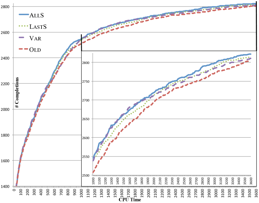
Figure 1: Cumulative number of instances completed by CPU time for POAC

For easy instances ($<100$ seconds), the completions of the strategies are similar. As the time limit increases Old becomes dominated by the other three strategies. To better compare AllS, LastS, and Var we examine the hard instances, zooming the chart on the cumulative CPU time solved between 1,000 and 3,600 seconds. Although Var performs well on smaller CPU time (Var contends with AllS for the most completed instances between 1,000 and 1,700 seconds) it becomes dominated by AllS and LastS on the harder instances. AllS clearly dominates all other strategies. These curves confirm the results of the statistical analysis given in Table 1.

4.3 Relational Neighborhood Inverse Consistency

The statistical analysis compares the relative performance for Old, AllC, and Head for RNIC. It shows that, overall, AllC and Head are equivalent and Old has the worst performance. The following holds in general for all benchmarks:

$$\textsc{AllC}\equiv\textsc{Head}>\textsc{Old}$$ (3)

The fact that Old is the worst demonstrates that RNIC’s contribution to the weights of dom/wdeg should not be ignored, thus justifying our investigations.

Table 5 summarizes the experiments’ results on all the 132 tested benchmarks. AllC is the best strategy on all measures while Old is the worst.

Table 5: Results of experiments for RNIC

Old AllC Head # Completion (3,869) 2,420 2,427 2,423 $\sum$CPU sec. (2,416) $>$1,032,130 $>$1,010,221 $>$1,014,635 Average NV (2,432) 77,067 45,696 45,803

We were not able to uncover meaningful categories of benchmarks to distinguish between AllC and Head. Table 6 summarizes individual benchmark results for the Dimacs category.

Table 6: Examples of Dimacs benchmarks where AllC and Head perform best

Benchmark Old AllC Head pret Completion (8) 4 4 4 $\Sigma$CPU (4) 196 28 61 Average NV (4) 1,285,234 125,793 273,736 dubois Completion (13) 6 9 11 $\Sigma$CPU (6) $>$22,041 $>$10,088 1,348 Average NV (11) 11,222,349 1,522,902 382,329

Within the category, either AllC or Head perform the best by all measures on different benchmarks. Similar results are obtained on the graph coloring category, shown in Table 7.

Table 7: Two graph coloring benchmarks where AllC and Head perform best

Benchmark Old AllC Head mug Completion (8) 8 8 8 $\Sigma$CPU (8) 5,098 548 2,819 Average NV (8) 1,501,379 189,595 883,130 leighton-15 Completion (26) 5 5 5 $\Sigma$CPU (5) 2,219 1,493 1,222 Average NV (5) 25,014 12,461 4,972

Having such different results between AllC and Head explains why the statistical analysis found them to be equivalent. Regardless, either AllC or Head performs better than Old in a statistically significant manner.

Figure 2 shows the cumulative number of instances completed by each strategy as CPU time increases.

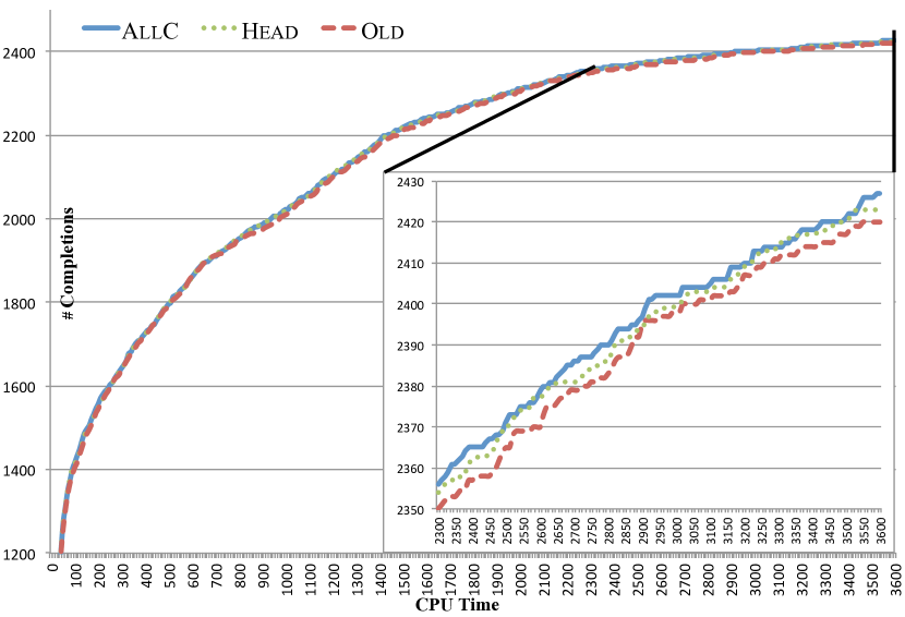
Figure 2: Cumulative number of instances completed by CPU time for RNIC

As was the case for POAC, on easy instances ($<100$ seconds), the completions of the strategies are similar. Focusing on harder instances, solved between 2,300 and 3,600 seconds, Old becomes dominated by AllC and Head. The curves of AllC and Head remain close to one another. These curves confirm the ranking in Equation 3.

5 Conclusion

This paper introduces four strategies for incrementing the weight in dom/wdeg for singleton consistencies (POAC) and three strategies for relational consistencies (RNIC). For both consistencies, Old is the worst strategy and a weighting schema involving the higher-level consistency is necessary. We show that for POAC the best method is AllS, which increments the weights at every singleton test. For RNIC, we show AllC and Head are statistically equivalent. Our work is a first step in the right direction, especially given the importance of higher-level consistencies in solving difficult CSPs. Future work may need to investigate more complex strategies for these and other consistencies.

References

- [Balafrej et al., 2014] Amine Balafrej, Christian Bessiere, El-Houssine Bouyakhf, and Gilles Trombettoni. Adaptive Singleton-Based Consistencies. In Proc. of AAAI 2014, pages 2601–2607, 2014.
- [Bennaceur and Affane, 2001] Hachemi Bennaceur and Mohamed-Salah Affane. Partition-k-AC: An Efficient Filtering Technique Combining Domain Partition and Arc Consistency. In Proc. of CP 2001, volume 2239 of LNCS, pages 560–564, 2001.
- [Bitner and Reingold, 1975] James R. Bitner and Edward M. Reingold. Backtrack Programming Techniques. Communications of the ACM, 18(11):651–656, November 1975.
- [Boussemart et al., 2004] Frédéric Boussemart, Fred Hemery, Christophe Lecoutre, and Lakhdar Sais. Boosting Systematic Search by Weighting Constraints. In Proc. of ECAI 2004, pages 146–150, 2004.
- [Debruyne and Bessière, 1997] Romuald Debruyne and Christian Bessière. Some Practicable Filtering Techniques for the Constraint Satisfaction Problem. In IJCAI 1997, pages 412–417, 1997.
- [Freuder and Elfe, 1996] Eugene C. Freuder and Charles D. Elfe. Neighborhood Inverse Consistency Preprocessing. In Proc. of AAAI 1996, pages 202–208, 1996.
- [Lecoutre, 2011] Christophe Lecoutre. STR2: Optimized Simple Tabular Reduction for Table Constraints. Constraints, 16(4):341–371, 2011.
- [Mackworth, 1977] Alan K. Mackworth. On Reading Sketch Maps. In Proc. of IJCAI 77, pages 598–606, 1977.
- [Michel and Van Hentenryck, 2012] Laurent Michel and Pascal Van Hentenryck. Activity-Based Search for Black-Box Constraint Programming Solvers. In Proc. of CPAIOR 2012, volume 7298, pages 228–243. Spring, 2012.
- [Palmieri et al., 2016] Anthony Palmieri, Jean-Charles Régin, and Pierre Schaus. Parallel Strategies Selection. In Proc. of CP 2016, volume 9892 of LNCS, pages 388–404. Springer, 2016.
- [Refalo, 2004] Philippe Refalo. Impact-Based Search Strategies for Constraint Programming. In Proc. of CP 2004, volume 3258 of LNCS, pages 557–571. Springer, 2004.
- [Vion et al., 2011] Julien Vion, Thierry Petit, and Narendra Jussien. Integrating Strong Local Consistencies into Constraint Solvers. In 14th Annual ERCIM International Workshop on Constraint Solving and Constraint Logic Programming, CSCLP 2009, volume 6080 of LNAI, pages 90–104. Springer, 2011.
- [Wallace and Freuder, 1992] Richard J. Wallace and Eugene C. Freuder. Ordering Heuristics for Arc Consistency Algorithms. In AI/GI/VI 92, pages 163–169, 1992.
- [Wilcoxon, 1945] Frank Wilcoxon. Individual Comparisons by Ranking Methods. Biometrics Bulletin, 1(6):80–83, 1945.
- [Woodward et al., 2011] Robert Woodward, Shant Karakashian, Berthe Y. Choueiry, and Christian Bessiere. Solving Difficult CSPs with Relational Neighborhood Inverse Consistency. In Proc. of AAAI 11, pages 112–119, 2011.
- [Woodward et al., 2012] Robert J. Woodward, Shant Karakashian, Berthe Y. Choueiry, and Christian Bessiere. Revisiting Neighborhood Inverse Consistency on Binary CSPs. In Proc. of CP 2012, volume 7514 of LNCS, pages 688–703. Springer, 2012.