No surviving companion in Kepler’s supernova

Abstract

We have surveyed Kepler’s supernova remnant in search of the companion star of the explosion. We have gone as deep as 2.6 $L_{\odot}$ in all stars within 20% of the radius of the remnant. We use FLAMES at the VLT-UT2 telescope to obtain high resolution spectra of the stellar candidates selected from HST images. The resulting set of stellar parameters suggests that these stars come from a rather ordinary mixture of field stars (mostly giants). A few of the stars seem to have low [Fe/H] ($<$ -1) and they are consistent with being metal-poor giants. The radial velocities and rotational velocities $v_{rot}$ sin $i$ are very well determined. There are no fast rotating stars as $v_{rot}$ sin i $<$ 20 km s^-1 for all the candidates. The radial velocities from the spectra and the proper motions determined from HST images are compatible with those expected from the Besançon model of the Galaxy. The strong limits placed on luminosity suggest that this supernova could have arisen either from the core-degenerate scenario or from the double-degenerate scenario.

1. Introduction

The supernova of 1604, observed by Johannes Kepler and other European, Korean, and Chinese astronomers, is one of the five “historical” supernovae that have been classified as belonging to the Type Ia (thermonuclear), the other four being SN 1572 (Tycho Brahe’s SN), SN 1006, SN 185 (supposed to have created the remnant RCW86) and the recently discovered youngest SNIa G1.9+03 that occurred in our Galaxy as recently as around 1900 but was not discovered due to dust exctinction and being only observable from the Southern hemisphere.

As it is well known, Type Ia SN (SNe Ia) are well explained by the thermonuclear explosion of a mass–accreting C+O white dwarf star (WD), a member of a close binary system, the mass donor being the other component of the system. There are three proposed channels to bring the WD to the point of explosion, depending on the nature of the companion star. In the single–degenerate channel (SD), the companion is a still thermonuclearly evolving star (Whelan & Iben 1973; Nomoto 1982), in the double–degenerate (DD) channel it is another WD, either a C+O WD or a He WD (Iben & Tutukov 1984; Webbink 1984). Another possible channel, known as the core–degenerate scenario (CD), involves a C+O WD that merges with the core of an Asymptotic Giant Branch (AGB) star, following a common–envelope episode (Livio & Riess 2003; Soker, García–Berro & Althaus 2014; Aznar-Siguán et al. 2015).

Significant progress has been done in the identification of progenitors of Type Ia supernovae (hereafter SNe Ia). For instance, there has been proof of an specific scenario that works to give rise to SNe Ia. This is the double detonation scenario studied theoretically by Fink et al. (2010); Sim et al (2012) and others. In this scenario, the CO WD accumulates a helium–rich layer on in its surface. The detonation of the helium–rich layer ignites the CO WD. This seems to be the explosion mechanism involved in MUSSES1604D (Jiang et al. 2017) and similar events. A He WD companion seems to be favored. The donor He-rich WD might survive in particular cases studied by Shen & Schwab (2017).

However, the observed double detonation scenario, as seen from the effect in the very early light curves of the SNe Ia, can not account for more than a small percentage of the SNe Ia observed (Jiang et al. 2017).

Another possible path to SNe Ia is the WD–WD collision. In this new DD path, no surviving companion is expected. A study of this mechanism to give rise to SNe Ia shows that would account for $<$ 1% of the observed events (see Soker 2018 for an overview).

So, mainly in the single degenerate scenario, a surviving companion should remain after the explosion. There is no surviving companion, but merging of the two components of the system in the DD scenario and in the CD scenario. On the contrary, in the SD channel, the companion star should survive the SN explosion. A surviving companion might be identified from its kinematics (large radial velocity and/or proper motion, fast rotation), anomalous luminosity, or contamination of its surface layers by the SN ejecta (Wang & Han 2012; Ruiz-Lapuente 2014 review those effects). Detailed simulations can be found in Marietta, Burrows & Fryxell (2000); Podsiadlowski (2003); Pakmor et al. (2008); Pan, Ricker & Taam (2012,2013,2014); Liu et al. (2012, 2013); Shapee, Kochanek & Stanek (2013); Shen & Schwab (2017). We will compare observations with their predictions.

The central regions of the SNR of Tycho SN (Ruiz-Lapuente et al. 2004; González Hernández et al. 2009; Kerzendorf et al. 2009, 2013; Bedin et al. 2014) and of SN 1006 (González Hernández et al. 2012; Kerzendorf et al. 2012, 2018) have already been explored, to search for a possible surviving companion of the SN, as well as extragalactic remnants like SNR 0509-67.5 (Schaefer & Pagnotta 2012), SNR 0509-68.7 (Edwards et al. 2013), and N103B (Pagnotta & Schaefer 2015; Li et al. 2017). Studies of other SNRs are in progress or have been proposed. Through comparison of the work done by various authors in those SNR, the double degenerate scenario seems favored in several SNe Ia.

The classification of Kepler SN, SN 1604, as a SN Ia was a matter of debate for a long time, some authors classified it as a core–collapse SN, in spite of its position, quite above the Galactic plane. The question has been settled by X–-ray observations of the remnant (Cassam-Chenaï et al. 2004), showing an O/Fe ratio characteristic of SNe Ia (Reynolds et al. 2007).

There are indications (Vink 2008) that one component of the binary system giving rise to the SN might have created a detached circumstellar shell with a mass $\sim$ 1 M_⊙, expanding into the interstellar medium. More recently, Katsuda et al. (2015) have deduced that the shell should have lost contact with the binary years before the explosion. It has been suggested (Chiotellis et al. 2012; Vink 2016) that the companion star was an AGB star having lost its envelope at the time of the explosion.

The distance to the remnant has also been the object of discussion, the estimates ranging between 3 and 7 kpc. Thus, Reynoso & Goss (1999), based on the HI absorption towards the remnant, estimated 4.8 $<$ $d$ $<$ 6.2 kpc. Later, Sankrit et al. (2005), from the proper motion of the optical filaments, found $d$ = 3.9${}^{+1.4}_{-0.9}$ kpc. But very recently, Sankrit et al. (2016) have revisited their method and give $d$ = 5.1${}^{+0.8}_{-0.7}$ kpc. Even more recently, Ruiz-Lapuente (2017), from the reconstruction of the optical light curve of the SN based on the historical records, also infers a distance $d$ = 5.0$\pm$0.61 kpc, in agreement with Sankrit et al. (2016). We thus adopt here a distance d $\sim$ 5.0$\pm$ 0.7 kpc to Kepler SN. For that distance, given the Galactic latitude of the SNR, b = 6.8^o, it lies $\simeq$ 590 pc above the Galactic plane.

The aim of the paper is to address the progenitor system that led to Kepler’s supernova, SN 1604. A first paper on the possible progenitor of the Kepler supernova suggested a marginal possibility that there was a donor, but only tentatively (Kerzendorf et al. 2014, K14 hereafter). At that time, the Hubble Space Telescope (HST) proper motions were not analysed and the stellar parameters of the stars were unknown. Here we provide a complete analysis of a survey using the FLAMES instrument at the SN ESO VLT-UT2 and we add all the proper motion information from HST with a baseline of 10 years.

The present paper is organized as follows. Section 2 describes the search in Kepler and what can be obtained from it. Section 3 describes the observations done with the VLT using the FLAMES instrumentation and the reduction of those observations. It presents, as well, the proper motions obtained from data from the HST archive, from programmes GO-9731 and GO-12885 (P.I: Sankrit). Section 4 presents the method used to derive the stellar parameters and the results. Section 5 presents the estimated distances to the stars, and discusses the radial velocities obtained, comparing them to those in previous studies. Section 6 compares the candidate stars with a kinematical model of the Galaxy. Section 7 discusses the results and Section 8 provides a summary of the conclusions.

2. Survey for the progenitor of SN 1604

Our survey has a limiting apparent magnitude $m_{R}$ = +19 mag. The visual extinction $A_{V}$, in the direction to the remnant of Kepler’s SN is $A_{V}$ = 2.7$\pm$0.1 mag, and $A_{R}$/$A_{V}$ = 0.748. Thus, we have reached down to an absolute magnitude $M_{R}$ = +3.4 mag. That corresponds to a luminosity L = 2.6 L_⊙ . For the spectroscopic observations we used FLAMES (Pasquini et al. 2002) mounted to the UT2 of the VLT. For the measurement of the proper motions, we used archival data from the HST.

Table 1Names and coordinates of the candidate stars

Name	RA (J2000.0)	DC (J2000.0)
T01	17 30 39.700	-21 29 35.54
T02	17 30 39.713	-21 29 46.75
T03	17 30 40.626	-21 29 45.02
T04	17 30 40.161	-21 29 53.09
T05	17 30 41.397	-21 29 44.70
T06	17 30 40.566	-21 29 33.80
T07	17 30 40.732	-21 29 34.34
T08	17 30 40.617	-21 29 27.25
T09	17 30 40.953	-21 29 25.56
T10	17 30 40.897	-21 29 21.06
T11	17 30 40.222	-21 29 18.89
T12	17 30 40.337	-21 29 15.16
T13	17 30 40.707	-21 29 16.61
T14	17 30 41.083	-21 29 14.04
T14b	17 30 41.188	-21 29 15.32
T15	17 30 40.985	-21 29 11.13
T16	17 30 41.431	-21 29 06.22
T17	17 30 39.981	-21 29 05.86
T18	17 30 41.823	-21 29 16.92
T19	17 30 41.697	-21 29 25.99
T20	17 30 42.493	-21 29 36.22
T21	17 30 42.653	-21 29 31.49
T22	17 30 43.316	-21 29 24.04
T23	17 30 43.582	-21 29 16.96
T24	17 30 42.651	-21 29 13.80
T25	17 30 42.937	-21 29 52.31
T26	17 30 42.475	-21 29 52.90
T27	17 30 41.898	-21 30 04.20
T28	17 30 42.837	-21 29 45.08
T29	17 30 41.816	-21 30 08.89
T30	17 30 40.335	-21 30 06.24
T31	17 30 42.829	-21 29 02.77

As a comparison, Kerzendorf et al. (2014) performed a shallower survey of possible survivors down to L $>$ 10 L_⊙, according to them ( L $>$ 6 L_⊙, if we take our reliable newly determined distance to SN 1604).

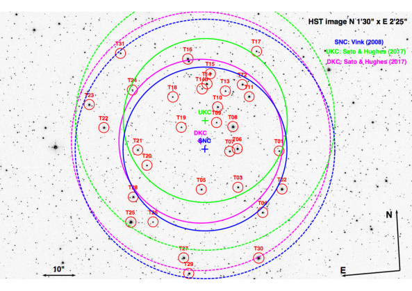
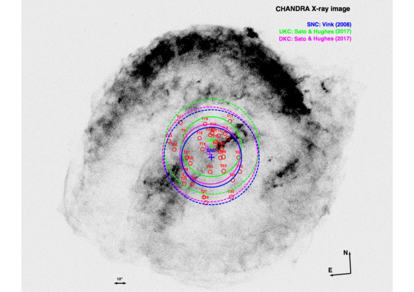
Figure 1.— Figure 1a. The targeted stars, in an image from the HST. Our adopted center of Kepler’s SNR, at $\alpha_{J200}$ = 17^h 30^m 41^s.25, $\delta_{J2000}$ = -21^o 2” 32”.95, is marked with a blue cross. We also provide the undecelerated (UKC, green) and decelerated (DKC, magenta) kinematic centers from Sato & Hughes (2017). The big (solid line) blue circle corresponds to a radius of 24 arcsec around the center SNC of the SNR, where our primary targets are located. The big (dashed) blue circle (of 38 arcsec) around SNC encompasses our supplementary targets (see text), and similarly for the circles around UKC and DKC. Figure 1b. Chandra X-ray image in the iron-rich 0.7-1.0 keV (Reynolds et al. 2007; Vink 2008) of the SN 1604, with the regions of search and labels in Figure 1a.

The remnant of SN 1604 has an average angular diameter of 225 arcsecs. Our survey is complete down to $m_{R}$ $\leq$ 19 within 24 arcsecs of the center of the SNR ($\simeq$ 20% of its radius: blue circumference in (Figure 1a), at $\alpha_{J2000}$ = 17^h 30^m 41^s.25, $\delta_{J2000}$ = -21^o 29’ 32”.95 (Vink 2008). Additional fibers were used to extend the search beyond 20% of its radius (the green circumference encompasses 38 arcsec of the radius), although the supplementary stars are not very relevant, due to their distances to the center of the SNR. The radius of the search area of 24 arcsec, at a distance of 5 kpc, corresponds to a transversal displacement from the center of the SNR by 0.58 pc. That is the path that a possible companion star would have travelled in 400 yr, moving at $v$ = 1460 km s^-1 perpendicularly to the line of sight. A total of 32 stars were observed. They are listed, with their coordinates, in Table 1.

While preparing the final version of this work, a new analysis of the X–ray knots of the Kepler SN by Sato & Hughes (2017) has provided as a result new estimates of the expansion center. Both are very close to the center that we used, by Vink (2008), thus it does not impact the results of the stars included in our search. There is an estimate that does not take into account a possible deceleration of the knots. This places the center at $\alpha_{J2000}$ = 17^h 30^m 41^s.189 $\pm$ 3.6^s and $\delta_{J2000}$ = -21^o 29’ 24”.63 $\pm$ 3.5”. The center that takes into account a deceleration coincides practically with that of Vink (2008). The newly determined center taking into account a model for the deceleration of the knots is $\alpha_{J2000}$ = 17^h 30^m 41^s.321 $\pm$ 4.4^s and $\delta_{J2000}$ = -21^o 29’ 30”.51 $\pm$ 4.3”. We include these new two centers in our Figure 1a. We include our search area in relation with the whole SNR in Figure 1b.

K14 explored the central region of Kepler’s SNR. The search has been photometric and spectroscopic, covering a square field of 38”x 38” around the center of the SNR determined by Katsuda et al. (2008), down to $m_{V}\simeq$ 18 mag. They have used, for their spectroscopy, the 2.3m telescope of the ANU, and for the photometry archival HST images. The WiFeS-spectrograph is an image slicer with 25 38X1” slitlets and 0.5” sampling in the spatial direction on the detector. They chose this instrument for its large field of view. However, that instrumentation did not allow to determine the stellar parameters. Apparently they noted that, due to sky subtraction errors, the continuum placement in their data was unreliable. Without determined stellar parameters, it is not possible to estimate distances, because the absolute magnitudes of the stars then remain unknown. They also had problems to estimate rotational velocities to better than 200 km s^-1 , due to the resolution and quality of the spectra (K14).

Here, we present a study that includes the stellar parameters, T_eff, log $g$ and [Fe/H]), and we also have rotational velocities and radial velocities, apart from the proper motions from HST. The conclusion on the supernova companion is thoroughly tested.

3. Observations

3.1. Spectral observations and reductions

Spectroscopic observations were secured with the multiobject spectrograph FLAMES (Pasquini et al. 2002) mounted at the Very Large Telescope (VLT) of the European Southern Observatory. Observations were made in the Combined IFU/7-Fibre simultaneous calibration UVES mode (Dekker et al. 2000) and Giraffe using the HR9 and HR15n settings under ESO programme ID 093.D-0384(A). The observations with UVES and Giraffe were done under clear sky and seeing conditions ranging from 0.78 to 1.88 arcsec (average of 1.28) from August 3rd to 25th 2014. FLAMES is the best instrument to use for our purpose, in particular Giraffe-IFU, since it provides the possibililty to observe within a very small field (24 and 38 arcsec in radius, blue and green circumferences in Figure 1) 32 targets to be obtained at the highest possible resolution and to minimize the requested observing time. 15 observing blocks (OBs) of 1 hour were prepared. Other modes of Giraffe as MEDUSA are not adequate for the amount of targets within a small circle of 24 arcsec (see Figure 1a as well as the separation between targets).

Observations of stars T2, T8, T25, T27, T29, and T30 were carried out with UVES using standard settings for the central wavelength of 580 nm in the red (covering from 476 to 684 nm with a 5 nm gap at 580 nm, and includes the H$\alpha$ feature). Giraffe observed stars T01-T031 (except stars T25, T27, T29 and T30) with both settings HR15n with central wavelength 665 nm in the red (covering from 647 nm to 679 nm) and HR9 with central wavelength 525.8 nm (covering from 509.5 nm to 540.4 nm).

From the abovementioned, we notice that stars T2 and T8 were observed both by UVES and Giraffe, providing a reliability test of these observations.

3.1.1 UVES observations and reductions

With an aperture on the sky of 1 arcsec, the fibers project onto five UVES pixels in the dispersion direction, giving a resolving power of $\sim$47000, enough to determine not only the radial and rotational velocities but the atmosphere parameters effective temperature, surface gravity and metallicity, T_eff, log $g$, and [Fe/H], of the stars.

The UVES reductions were done using the UVES pipeline version 5.5.2. Once individual spectra had been calibrated in wavelength, we corrected the spectra for the motion of the observatory to place them in the heliocentric reference system. Finally, we co-added the different exposures for each star by interpolating to a common wavelength array and computing the weighted mean using the errors at each wavelength as weights.

3.1.2 Giraffe observations and reductions

The Giraffe data were reduced using the dedicated ESO Giraffe pipeline, version 2.15¹⁰ and Giraffe Reflex workflow (Freudling et al. 2013), and calibration data provided by the ESO Science Archive Facility CalSelector tool. The obtained resolving power is $\sim$ 28000 for the HR9 grating and $\sim$ 30600 for the HR15n.

In most cases the default pipeline parameters resulted in a successful reduction, but in several the parameters of the flat field processing recipe had to be adjusted in order to achieve a successful reduction. In two cases it was not possible to find a set of parameters which allowed a successful reduction of the flat field, and in these cases the next nearest-in-time, successfully reduced flat was used instead.

Each individual science observation data file was corrected for cosmic-ray hits using a purpose written Python script based on the Astro-SCRAPPY (Pasquini et al. 2002) Python module. The cosmic-ray corrected science data files were processed individually with bias subtraction, flatfielding and wavelength calibration performed in the standard way by the pipeline and Reflex workflow. Subsequent reduction was then also performed in purpose written Python scripts.

A sky spectrum was then calculated for each science data file as the median of all individual sky-fibre spectra available in the file, typically 15 sky spectra. The resulting median sky-spectrum was then subtracted from the spectrum extracted for each IFU fibre.

As each star was observed with an IFU, its signal was thus distributed over several individual fibres, each of which is individually reduced and extracted by the pipeline. The S/N of each spectrum of a given IFU was then computed using the DERsnr algorithm, and the total signal for each star resulting from a single observation was then computed as the sum of the signal from $N$ highest S/N spectra, which maximised the S/N of the summed spectrum.

Each star in the sample was observed one to four times, depending on brightness. We checked that the spectra did not differ at different dates. The final spectrum for each star was then computed as a mean of the several dates. The wavelength scale of the resulting summed spectra for each star was then corrected to the heliocentric reference system.

3.2. Proper motions

To derive proper motions we used data from two HST programs collected at two epochs separated by almost 10 years.

Table 2The HST data used in this work

ACS/WFC	— epoch 1 —	2003.65842-2003.66141
F502N	4$\times$ $\sim$1100 s	GO-9731
F502N	4$\times$ $\sim$500 s	GO-9731
F660N	8$\times$ $\sim$500 s	GO-9731
F658N	4$\times$ $\sim$1250 s	GO-9731
F658N	4$\times$ $\sim$600 s	GO-9731
F550M	4$\times$ 210 s	GO-9731
WFC3/UVIS	— epoch 2 —	2013.50023-2013.50666
F336W	4$\times$ $\sim$750 s	GO-12885
F438W	4$\times$ $\sim$270 s	GO-12885
F547M	4$\times$ $\sim$470 s	GO-12885
F656N	8$\times$ $\sim$1220 s	GO-12885
F658N	4$\times$ $\sim$970 s	GO-12885
F814W	4$\times$ $\sim$240 s	GO-12885

The first epoch is the data-set from GO-9731 (PI: Sankrit), and it was collected in August 28-29 2003 with the Wide Field Channel (WFC) of the Advanced Camera for Surveys (ACS). The images are in three narrow-band filters F502N, F660N, F658N, and in one medium-band filter, F550M.

The second epoch is from GO-12885 (also PI: Sankrit), and it was collected in July 1-3 2013 with the UV-VISual Channel (UVIS) of the Wide Field Camera 3 (WFC3). The images are in F336W, F438W, F547M, F656N, F658N, and in F814W. We refer here to Table 2 for more details.

To derive proper motions we used 28 images in each of the two 10-year apart epochs. In Table 2 we give a log of the used images.

As the charge transfer efficiency (CTE) losses have a major impact on astrometric projects (Anderson & Bedin 2010), in this work every single AC/WFC and WFC3/UVIS image employed was treated with the pixel-based correction for imperfect CTE developed by Anderson & Bedin (2010). The improved corrections are directly included in the MAST dataproducts.

Raw positions and fluxes were extracted in every image using the software and the spatially variable effective point spread functions (PSFs) produced by Anderson & King (2006). All libraries PSFs for both ACS/WFC and WFC3/UVIS are publicly available.

The raw positions were then corrected for the average geometric distortion of these instruments using the prescriptions by Anderson (2002, 2007) for the ACS/WFC and by Bellini et al. (2009, 2011) for WFC3/UVIS.

The methodology and the procedures followed to derive proper motions were extensively described in a previous work with similar goals (Bedin et al. 2014). In the following we give a brief description.

We first defined a reference frame with respect to which we will measure all the relative positions. This was built using the four images in filter WFC3/UVIS/F814W from the second epoch, as they have the best image quality and highest number of stars with high signal. In the reference frame we used only relatively bright, unsaturated, isolated stars, and with a stellar profile (the quality fit $q$ described in Anderson et al. 2008).

Table 3Proper motions of the targeted stars

NAME	dRA(mas/yr)	dDC(mas/yr)	sRA(mas/yr)	sDC(mas/yr)
T01	0.96333105	3.42910032	0.12081037	0.07071602
T02	-2.33240031	3.86571195	45.22749329	54.34668660
T03	1.65005841	-0.00972573	0.03339045	0.08114443
T04	-4.85102345	-1.31896956	0.10271324	0.21623776
T05	2.78755994	0.98653555	0.06256493	0.08762565
T06	-0.14035101	0.80693946	0.06580537	0.08934278
T07	2.22968225	0.63820899	0.08311504	0.09635703
T08	-0.64593882	0.48014508	45.22705027	54.34598682
T09	1.15779958	0.38160776	0.11226873	0.09974361
T10	-1.17098183	-1.93729322	0.06072457	0.10494832
T11	1.07273546	1.85830604	0.07653632	0.12997579
T12	-1.84466939	-2.21716030	0.05498542	0.08621992
T13	0.82006479	3.46512561	0.05292586	0.06884338
T14	-3.85388310	1.59710464	0.10770873	0.10911011
T14b	2.19854365	-1.00379486	0.03274381	0.09097165
T15	-5.93215420	1.39310415	0.03482210	0.08710643
T16	0.29501700	5.03375451	0.02070014	0.05802598
T17	0.31106430	0.16393080	0.06300106	0.07123875
T18	25.06353304	-43.80675171	0.02033413	0.08582691
T19	-3.14334844	-4.36036079	0.05860900	0.08929045
T20	-0.81856961	1.70037126	0.06403092	0.04892372
T21	-3.56172476	-2.59434617	0.05555466	0.04844967
T22	1.63830144	-2.74355827	0.05628767	0.07366438
T23	7.54610667	-1.28547796	0.04192214	0.05333274
T24	-0.54450471	3.25364568	0.08436434	0.06721759
T25	0.16070871	-0.27626484	45.22705027	54.34598682
T26	-3.39922823	0.75818276	0.08496424	0.07949148
T27	2.52236058	4.58473159	0.04709384	0.08656006
T28	2.09224795	2.28248031	0.03391564	0.04773037
T29	2.81992271	-3.87317107	0.08391351	0.07822889
T30	2.37310197	7.78087136	45.22739769	54.34606942
T31	-2.61147871	-2.23889319	0.01148096	0.08836027

The positions from all these suitable stars measured in the four F814W images were then transformed into a common distortion corrected reference system and their clipped means taken as the final positions of the reference frame. The field is a relatively dense one, and the final reference frame is made of over 20 000 stars, giving a typical distance of $\sim$30 pixels to one such reference star. The consistency in the positions of the four F814W images gives a positional accuracy of $\sim$0.01 pixels for the brightest unsaturated sources; perfectly consistent with the accuracy given in the Bellini et al. (2011) geometric distortion, and as achieved in other work (for example, Bedin et al. 2013).

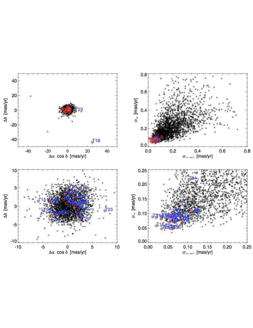
Figure 2.— Vector–point diagrams (left panels) of the proper motions measured and their errors (right panels). The lower panels are close–ups of the upper ones. Note the very high proper motion of T18 and, to a lesser degree, of T23.

To calibrate our reference frame we need to derive the astrometric zero points, plate scale, orientation, and skew terms, which are needed to bring its coordinate systems into an absolute astrometric system. To achieve this we used 266 sources in common between our reference frame and the 2MASS catalog (Skrutskie et al. 2006).

Hereafter our absolute coordinates will be given in equatorial coordinates at equinox J2000, with positions given at the reference epoch of the reference frame, 2013.50. Finally, we note that our absolute accuracy will be the same of the 2MASS catalog, about 0.2 arcsec, while our relative precisons should be much better than that, down to few 0.1 mas.

As in Bedin et al. (2014), we have also produced image stacks, which provide often a useful representation of the astronomical scene. There are 4+6 of such stacks, one per filter/epoch, and they give a critical inspection of the region surrounding each star at any given epoch.

We also produced trichromatic exposures for both epochs.

As extensively explained in Bedin et al. (2014), even the best geometric distortion available is always an average solution. There are always deviations from that, typically as large as $\sim$mas. To remove these residual systematic errors in our geometric distortion, we used the “bore-sight” correction described in detail in Bedin et al. (2014), which is essentially a local approach (Bedin et al. 2003). We used a network of at least 15 stars at no more than 500 pixels from target stars, used only stars with consistent positions between the two epochs better than 0.75 pixels, and stars brigher than at least 250 photo-electrons above the local sky.

Note that although most of the field objects are background Galactic bulge stars at $\sim$ 8 kpc, with an intrinsic dispersion of about $\sim$ 3 mas yr^-1 (e.g., Bedin et al. 2003), our proper motion precision in the catalogue is significantly superior to this limit. Indeed, motions of the references local net are averaged over N reference stars, implying systematics lowering by the factor $\sim$ 1/$\sqrt{(N-1)}$, with N typically ranging in the few hundreds and hardcoded to be at minimum 15.

To compute proper motions, we divide the measured displacements of sources between epoch 2 and epoch 1, by the time baseline after having transformed the displacements in the astrometric reference frame provided by the sources in our reference frame and 2MASS.

The proper motions are shown in Figure 2 and in Table 3. The uncertainties were computed as the sum in quadrature of the r.m.s. of positions observed within each of the two epochs.

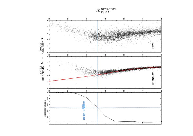
Figure 3.— Completeness in magnitude of the stars in the field of SN1604.

To assess the completeness of the measured sample in our field we calibrated our instrumental magnitudes and then perform artificial star tests.

The photometric calibration was performed only in filters ACS/WFC/F550M (narrow $V$) and WFC3/UVIS/F814W (wide $I$) and was obtained following the detailed procedures described in Bedin et al. (2005). We used the most updated zero points, which were adopted following STScI instructions. The calibrated CMD of the detected sources is shown in left panel of Fig.3.

Artificial star tests were performed as described in great detail in Anderson et al. (2008) for ACS/WFC, and more recently applied to WFC3/UVIS detectors (e.g., Bedin et al. 2015). Briefly, we built a fiducial line of the “main” Main-Sequence of the galactic field stars as representative for the sources in the field (middle panel of Fig.3), and add those sources in the individual images, which were reduced in identical manner to the real sources. The ratio between the number of recovered and the inserted artificial stars at variuous instrumental magnitude levels then provide the completness curve, which is shown on right panel of Fig. 3.

We can be reasonably confident that our sample is virtually complete down to $m_{\rm F814W}\simeq 22.5$, and 50$\%$—complete down to $\sim$23.4. However, completeness has always a statistical value, as individual stars can be missed for several reasons.

4. Stellar parameters

The stellar parameters T_eff, log $g$, and [Fe/H] have been determined, from the spectra obtained with the Giraffe spectrograph in the HR15n setup and from the UVES spectra in the 580nm setup, through the spectroscopic indices defined by Damiani et al. (2014). The method is based on a set of narrow-band spectral indices, and calibrated stellar parameters are derived from suitable combinations of these indices. Those indices sample the amplitude of the TiO bands, the H$\alpha$ core and wings, and temperature- and gravity-sensitive sets of lines at several wavelength intervals. The latter are the close group of lines between 6490-6500 Å, which are sensitive to gravity, and Fe I lines falling within the range covered by the HR15 setup, that are sensitive to temperature. Further gravity-sensitive features are found in the 6750-6780 Å  region.

Two global indices, $\tau$ (sensitive to temperature) and $\gamma$ (gravity-sensitive), are computed from the former ones. A further composite index, $\zeta$, measures stellar metallicity.

Tests and calibrations of those indices have been performed (Damiani et al. 2014), based on photometry and reference spectra from the UVES Paranal Observatory Project (Bagnulo et al. 2003) and the ELODIE 3.1 Library (Prugniel & Soubiran 2001).

Table 4Stellar surface parameters of the targeted stars

Star	$v_{r}$ (km/s)	$v_{rot}\ {\rm sin}\ i$ (km/s)	Teff (K)	Teff err.	log $g$	log $g$ err.	[Fe/H]	[Fe/H] err.
T01	34.1	14.2	4872	321	2.8	0.9	-0.4	0.3
T02	43.9	14.2	3911	152	0.6	1.1	-1.1	0.4
T03	140.8	14.5	4415	199	2.3	0.8	0.1	0.2
T04	8.2	15.5	5545	251	3.8	0.6	0.1	0.1
T05	35.1	14.7	4053	246	0.8	1.6	-1.1	0.6
T06	94.4	14.2	4270	196	2.1	0.8	0.0	0.2
T07	-47.6	17.1	6243	202	3.5	0.5	0.7	0.1
T08	-84.6	15.3	4633	159	1.9	0.5	-0.2	0.1
T09	-15.8	13.0	4890	549	4.3	1.0	-0.4	0.5
T10	-17.1	14.7	4252	191	2.0	0.8	-0.2	0.2
T11	-83.3	13.9	4000	155	1.0	0.8	-0.4	0.3
T12	-148.0	18.6	4089	192	0.9	1.0	-0.7	0.4
T13	-4.8	13.8	4627	286	1.6	0.9	0.2	0.2
T14	-81.3	15.0	4295	143	1.7	0.6	-0.4	0.2
T14b	142.3	12.9	4396	235	3.2	0.7	-0.0	0.3
T15	-23.2	16.4	4979	284	4.5	1.2	0.2	0.1
T16	-89.7	14.3	4760	171	1.9	0.5	-0.3	0.1
T17	-125.8	14.9	4540	365	—-	—-	—-	—-
T18	42.4	12.3	3777	28	4.5	0.2	—-	—-
T19	8.6	14.8	4505	351	—-	—-	-2.2	1.6
T20	26.3	13.8	3874	185	1.5	1.3	-1.1	0.5
T21	11.0	15.9	4673	189	2.0	0.6	-0.4	0.2
T22	106.8	17.5	5164	159	2.0	0.4	-0.4	0.1
T23	50.8	15.6	5436	336	5.3	1.6	-1.2	0.5
T24	38.2	12.4	4237	198	3.2	0.7	-1.2	0.8
T25	45.3	20.0	4414	293	—-	—-	—-	—-
T26	-87.5	16.9	3619	316	—-	—-	-3.8	18.9
T27	-68.3	10.7	4971	341	1.1	1.2	-1.0	0.4
T28	51.0	14.8	4448	170	2.1	0.7	-1.0	0.3
T29	45.4	11.3	4034	135	2.9	0.5	-0.7	0.5
T30	54.8	11.1	4237	179	1.3	1.0	-1.3	0.4
T31	-67.5	16.1	4825	268	3.0	0.8	-0.4	0.2

The method works well for stars in the approximate temperature range 3,000 K $\,\buildrel<\over{\sim}\,$ T_eff $\,\buildrel<\over{\sim}\,$ 9,000 K. The values of T_eff, log $g$, and [Fe/H], with their errors, for our targeted stars, are given in columns 4-9 of Table 4. There were 4 stars (T17, T19, T25, and T26) whose surface gravities could not be determined in this way, due to the low S/N of their spectra. Their distances are thus left largely undetermined. We know their effective temperatures, however, and so we can estimate the distance depending on the luminosity classes to which they can belong.

The resulting set of stellar parameters suggests that the stars come from a rather ordinary mixture of field stars (mostly giants). A few of the stars seem to have low [Fe/H] ($<$ -1), although with large errors; they are all consistent with being metal-poor giants. The radial velocities and the rotational $v$ sin $i$ values are very well determined. Radial velocities were measured from several lines in the spectra of the targeted stars. All spectra gave a clear and narrow peak in the cross-correlation function (CCF) with template spectra. Even when spectral lines are poorly defined, the CCF may be sharply peaked, since all lines add up. Radial and rotational velocities were measured from the CCF, as above, using a set of template spectra covering the relevant T_eff range, taken from the Gaia–ESO sample studied in Damiani et al. (2014); the template giving the highest CCF peak for each program star was used for the velocity determinations, an approach well-tested within the Gaia-ESO Survey. The radial velocities and $v$ sin $i$ values are very well determined and their errors (i.e. uncertainties on CCF peak center and width) lower in percentage than the errors in the stellar parameters. Uncertainties on radial and rotational velocities based on Giraffe data were carefully studied by Jackson et al. (2015), and found to be dependent on S/N, T_eff and $v$ sin $i$ (besides, obviously, of spectral resolution). For the ranges of these parameters relevant to this work, this implies typical uncertainties of 1-2 km/s on radial velocities, and 10-15 km/s on $v$ sin $i$.

T18 is a clear outlier having very fast motion across the line of sight. However, this star is just a cold, M-dwarf, located at around half a kpc away only.

5. Distances and radial velocities

By comparison of the stellar parameters with the observed apparent magnitudes in different bands, the distances to the targeted stars are determined. We use, for that, the isochrones of Marigo et al. (2017) (see Fig. 4 for an example), which

Figure 4.— The target star T04 plotted in the T_eff–log $g$ diagram, superimposed on the isochrones of Marigo et al. (2017). The isochrones are labeled in Gyrs.

give, for each combination of the parameters T_eff, log $g$, and [Fe/H], the absolute magnitudes M_V, M_R, M_J, M_H, and M_K. Apparent magnitudes of the stars in our sample are taken from the NOMAD catalog, and compared with the absolute magnitudes in the different photometric bands, taking into account the corresponding extinctions. The results are given in Table 5. The distances indicated, with their errors, are weighted averages over the different bands.

Table 5Absolute magnitudes of the targeted stars, observed apparent magnitudes, and inferred distances

Star	MV	mV	MR	mR	MJ	mJ	MH	mH	MK	mK	d (kpc)
T01	1.1${}^{+1.5}_{-2.2}$		0.5${}^{+1.4}_{-2.2}$	17.9	-0.5${}^{+1.3}_{-2.1}$	15.4	-1.0${}^{+1.2}_{-2.1}$	14.8	-1.1${}^{+1.3}_{-2.0}$	14.5	11.5${}^{+17}_{-5.1}$
T02	-4.3${}^{+6.0}_{-0.7}$		-5.2${}^{+6.4}_{-0.7}$	16.0	-7.1${}^{+7.1}_{-0.6}$		-7.9${}^{+7.3}_{-0.4}$		-8.1${}^{+7.4}_{-0.4}$		$>$20
T03	1.2${}^{+2.2}_{-2.8}$		0.5${}^{+2.2}_{-2.8}$	16.2	-0.8${}^{+2.1}_{-2.7}$	14.3	-1.5${}^{+2.0}_{-2.6}$	13.6	-1.6${}^{+2.0}_{-2.6}$	13.3	8.2${}^{+20}_{-2.3}$
T04	3.3${}^{+1.9}_{-0.7}$		2.9${}^{+1.9}_{-0.9}$	15.9	2.2${}^{+1.9}_{-1.2}$	15.1	1.7${}^{+1.9}_{-1.3}$	14.5	1.6${}^{+1.9}_{-1.3}$	14.5	3.3${}^{+2.7}_{-1.9}$
T05	-4.6${}^{+4.4}_{-1.8}$		-5.4${}^{+4.3}_{-1.8}$	17.5	-7.0${}^{+4.1}_{-1.6}$	14.9	-7.7${}^{+4.0}_{-1.5}$	14.1	-7.9${}^{+4.0}_{-1.5}$	14.0	$>$20
T06	0.8${}^{+2.4}_{-2.6}$	16.3	0.1${}^{+2.3}_{-2.5}$		-1.3${}^{+2.3}_{-2.4}$	13.7	-2.0${}^{+2.5}_{-2.5}$	13.0	-2.1${}^{+2.3}_{-2.5}$	12.7	8.0${}^{+17}_{-5.3}$
T07	1.5${}^{+1.9}_{-1.1}$		1.2${}^{+1.8}_{-1.1}$	19.3	0.6${}^{+1.8}_{-1.0}$		0.3${}^{+1.8}_{-1.0}$		0.3${}^{+1.8}_{-1.0}$		16${}^{+11}_{-9}$
T08	0.6${}^{+1.1}_{-1.0}$	15.9	-0.3${}^{+0.7}_{-0.7}$	12.8	-1.1${}^{+0.9}_{-0.9}$	13.1	-1.9${}^{+0.7}_{-0.7}$	12.3	-2.0${}^{+0.7}_{-0.7}$	12.0	5.5${}^{+2.0}_{-1.5}$
T09	4.7${}^{+4.5}_{-1.1}$		4.3${}^{+4.0}_{-1.1}$		3.5${}^{+2.7}_{-1.2}$	15.4	3.2${}^{+2.4}_{-1.3}$	14.6	3.1${}^{+2.3}_{-1.3}$	14.3	1.5${}^{+2.0}_{-1.0}$
T10	0.7${}^{+2.3}_{-2.9}$		0.0${}^{+2.2}_{-2.9}$	15.9	-1.4${}^{+2.1}_{-2.8}$	14.9	-2.1${}^{+2.2}_{-2.8}$	13.7	-2.2${}^{+2.1}_{-2.8}$	13.4	12${}^{+32}_{-4.0}$
T11	-2.7${}^{+2.5}_{-3.0}$	16.2	-3.5${}^{+2.5}_{-2.9}$	13.0	-5.3${}^{+2.5}_{-2.8}$	14.0	-6.0${}^{+2.4}_{-2.7}$	13.2	-6.2${}^{+2.4}_{-2.7}$	13.0	$>$20
T12	-4.0${}^{+3.1}_{-2.8}$	16.4	-4.8${}^{+3.3}_{-2.4}$		-6.4${}^{+2.7}_{-2.6}$	14.8	-7.1${}^{+2.6}_{-2.8}$	14.2	-7.3${}^{+2.7}_{-2.6}$	14.1	$>$20
T13	-2.7${}^{+2.7}_{-2.6}$		-3.3${}^{+2.6}_{-2.4}$	17.7	-4.5${}^{+2.5}_{-2.3}$	15.0	-5.1${}^{+2.5}_{-2.2}$	14.2	-5.2${}^{+2.5}_{-2.2}$	14.0	$>$20
T14	-1.1${}^{+1.6}_{-1.6}$	16.7	-1.8${}^{+1.6}_{-1.6}$	13.9	-3.3${}^{+1.6}_{-1.6}$	14.0	-3.9${}^{+1.5}_{-1.6}$	13.2	-4.1${}^{+1.6}_{-1.6}$	12.9	21${}^{+25}_{-10}$
T14b	2.8${}^{+2.3}_{-1.0}$		2.3${}^{+2.4}_{-1.1}$	17.4	1.1${}^{+2.1}_{-1.1}$	15.4	0.6${}^{+2.1}_{-1.2}$	14.8	0.5${}^{+2.1}_{-1.2}$	14.5	5.5${}^{+4.0}_{-3.4}$
T15	5.7${}^{+2.8}_{-3.2}$	16.7	5.3${}^{+2.3}_{-3.3}$	13.9	4.3${}^{+1.6}_{-3.3}$		3.9${}^{+1.3}_{-3.5}$	13.2	3.8${}^{+1.2}_{-3.5}$	12.9	0.6${}^{+2.2}_{-0.3}$
T16	-2.0${}^{+2.5}_{-1.8}$	16.1	-2.6${}^{+2.5}_{-1.8}$	15.3	-5.8${}^{+2.4}_{-1.8}$	13.6	-4.3${}^{+2.3}_{-1.8}$	12.9	-4.4${}^{+2.4}_{-1.8}$	12.6	22${}^{+27}_{-15}$
T17				17.1		15.3		14.4		14.2
T18	8.6${}^{+0.1}_{-0.4}$		7.6${}^{+0.2}_{-0.5}$	17.6	5.6${}^{+0.4}_{-0.5}$	15.1	5.0${}^{+0.4}_{-0.5}$	14.5	4.8${}^{+0.4}_{-0.5}$	14.2	0.6${}^{+0.2}_{-0.1}$
T19				17.9		15.6		14.9		14.6
T20	0.0${}^{+3.8}_{-5.7}$		-0.8${}^{+3.7}_{-5.7}$	17.2	-2.5${}^{+3.6}_{-5.6}$	15.3	-3.3${}^{+3.6}_{-5.5}$	14.5	-3.4${}^{+3.5}_{-5.5}$	14.3	$>$20
T21	-1.6${}^{+2.6}_{-1.3}$	17.7	-2.2${}^{+2.6}_{-1.3}$	16.7	-3.4${}^{+2.6}_{-1.2}$	14.7	-3.9${}^{+2.6}_{-1.2}$	13.9	-4.0${}^{+2.6}_{-1.1}$	13.6	29${}^{+20}_{-27}$
T22	-2.5${}^{+1.7}_{-0.9}$	16.3	-2.9${}^{+1.6}_{-0.9}$	17.0	-3.9${}^{+1.5}_{-0.8}$	14.1	-4.3${}^{+1.5}_{-0.8}$	13.4	-4.4${}^{+1.5}_{-0.7}$	13.2	28${}^{+11}_{-14}$
T23	9.9${}^{+4.3}_{-7.8}$	16.3	8.9${}^{+4.3}_{-7.1}$	15.4	6.6${}^{+4.1}_{-5.5}$	14.6	6.0${}^{4.0+}_{-5.1}$	14.0	5.8${}^{+4.0}_{-4.9}$	13.8	0.3${}^{+3.0}_{-0.2}$
T24	4.3${}^{+2.1}_{-2.0}$		3.2${}^{+2.0}_{-1.9}$	17.8	2.0${}^{+2.0}_{-1.8}$	15.4	1.4${}^{+2.0}_{-1.8}$	14.8	1.3${}^{+1.9}_{-2.2}$	14.4	3.8${}^{+6.8}_{-2.2}$
T25						12.7		12.0		11.8
T26						15.6		15.1		14.8
T27	-5.6${}^{+5.4}_{-3.3}$	16.2	-6.1${}^{+5.2}_{-3.2}$		-7.0${}^{+5.0}_{-3.1}$	14.2	-7.4${}^{+4.8}_{-3.6}$	13.7	-7.5${}^{+4.8}_{-3.1}$	13.5	$>$20
T28	0.0${}^{+1.1}_{-2.2}$		-0.7${}^{+1.1}_{-1.9}$		-2.0${}^{+1.0}_{-2.0}$	13.9	-2.7${}^{+1.1}_{-2.0}$	13.3	-2.8${}^{+1.1}_{-2.0}$	13.1	13${}^{+20}_{-5.0}$
T29	4.1${}^{+1.7}_{-1.6}$		3.0${}^{+1.5}_{-1.6}$		1.7${}^{+1.3}_{-1.5}$	13.8	1.1${}^{+1.2}_{-1.5}$	13.0	1.0${}^{+1.1}_{-1.5}$	12.8	2.1${}^{+2.1}_{-0.8}$
T30	-3.0${}^{+3.4}_{-3.0}$	15.4	-3.7${}^{+3.3}_{-3.0}$	14.9	-5.2${}^{+3.3}_{-2.9}$	14.0	-5.9${}^{+3.3}_{-2.8}$	13.7	-6.0${}^{+3.2}_{-2.9}$	13.4	$>$20
T31	2.1${}^{+0.7}_{-3.0}$		1.4${}^{+0.8}_{-2.9}$	17.8	0.3${}^{+0.7}_{-2.5}$	15.8	-0.3${}^{+0.8}_{-2.2}$	14.9	-0.3${}^{+0.7}_{-2.2}$	14.9	9.6${}^{+17}_{-2.7}$

Peculiar radial velocities, as referred to the average velocities of the stars at the same position in the Galaxy, can be one characteristic of a surviving companion of the SN, the excess velocity coming from the orbital motion of the star before the binary system is disrupted by the explosion, plus the kick imparted by the collision with the SN ejecta.

Table 6Radial velocities measured in this work and in K14

Star	$v_{r}$ (km/s)a	K14	$v_{r}$ (km/s)
T01	34.1
T02	43.9
T03	140.8
T04	8.2
T05	35.1
T06	94.4	P1	86.7
T07	-47.6	P2
T08	-84.6	L1	-88.29
T09	-15.8	G1	-94.29
T10	-17.1	F1	-10.51
T11	-83.3	N1	-81.88
T12	-148.0	K1	-155.96
T13	-4.8	H1	177.58
T14	-81.3	B1
T14b	142.3	B2	167.17
T15	-23.2	D1	-74.27
T16	-89.7	E1	-38.64
T17	-125.8
T18	42.4	A1	-69.07
T19	8.6	C1	7.01
T20	26.3	R1	41.44
T21	11.0	O1	-10.71
T22	106.8
T23	50.8
T24	38.2
T25	45.3
T26	-87.5
T27	-68.3
T28	51.0
T29	45.4
T30	54.8
T31	-67.5	Q1	-59.06

^a The errors in the radial velocities are of 1–2 km s^-1.

The results are given in the first and second columns in Table 6, and they are compared with those of K14 for stars common to the two surveys in the third and fourth columns. The velocities are in the heliocentric system. There is good agreement for some stars but not for all of them. In our case, we have two or three spectra of the same star, so we can be sure about the radial velocities and exclude possible binarity of those stars. As an example, we can quote the velocity of our T18, star named A in K14. We measure its radial velocity with an uncertainty of 1-2 km s^-1. The star moves at 42.5 km s^-1, while K14 give -69.07 km s^-1.

We will address the point of radial velocities and proper motions as compared to the kinematics of the Galaxy in Section 6.

6. Comparison with model kinematics of the Galaxy

Being the surviving companion star of a SN Ia means to have a peculiar velocity, referred to the average velocity of the stars at the same position in the Galaxy, due to the orbital motion in the binary progenitor of the SN, plus the kick velocity caused by the impact of the SN ejecta. An estimate of the expected velocities, depending on the type of companion (main–sequence, subgiant, red giant, supergiant) was made by Canal et al. (2001), and more recently by Han (2008). The highest peculiar velocities ($\sim$ 450 km s^-1 ) would correspond to main-sequence companions and the smallest ones ($\sim$ 100 km s^-1) to red giants.

As the reference for the average velocities of the stars, depending on the location within the Galaxy and on the stellar population considered, we adopt the Besançon model of the Galaxy (Robin et al. 2003). We have run the model to find the distributions of both radial velocities and proper motions in the direction of the center of Kepler’s SNR and within the solid angle subtended by our search, and including all stellar populations. The same model has been taken as the reference in K14.

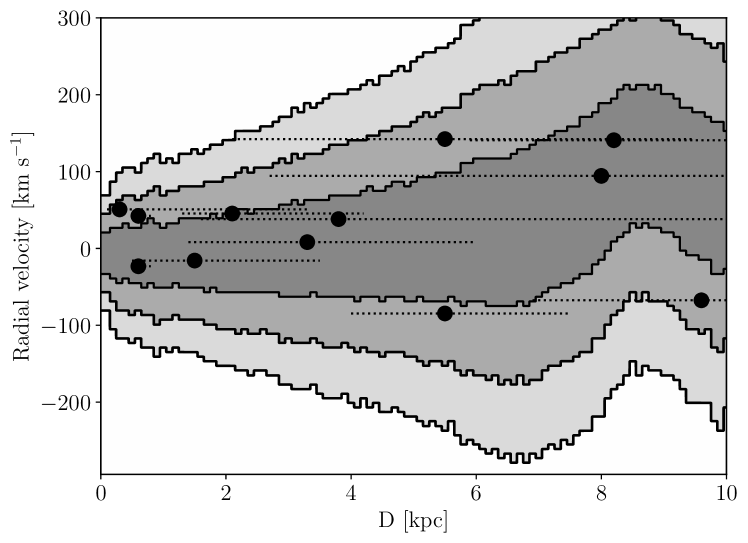
Figure 5.— The distances and radial velocities of the targeted stars with $d{\hbox{\lower 3.44444pt\hbox{$\,\buildrel<\over{\sim}\,$}}10}$ kpc, plotted over the distribution given by the Besançon model of the Galaxy. No star significantly deviates for the predicted distribution. We show 1 $\sigma$, 2 $\sigma$ and 3 $\sigma$ contours of the Galactic distribution of stars.

In Figure 5, the 1, 2, and 3 $\sigma$ regions of the radial-velocity distribution (in the heliocentric reference system) are shown. We see that the average velocities first steadily increase, with positive values. That corresponds to the differential rotation of the Galactic disc. The dispersion also increases as, given the direction of the line-of-sight, we move from the thin to the thick disc. Then, at a distance of $\sim$7 kpc, both the slope and the dispersion increase when reaching the Galactic bulge, to start decreasing beyond $\sim$9 kpc.

In the same Figure we compare the measured radial velocities with the distribution predicted by the Besançon model. We see that there is no star significantly deviating from the model distribution.

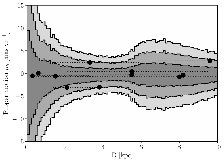
Figure 6.— Same as Figure 5, for the proper motions perpendicular to the Galactic plane $\mu_{b}$. Star T18, at a distance of 0.4 kpc only, is not shown here, it falling outside the scale of the plot.

In Figure 6, the same is done for the proper motions perpendicular to the Galactic plane. In Figure 7, the same is done for the proper motions in Galactic latitude.

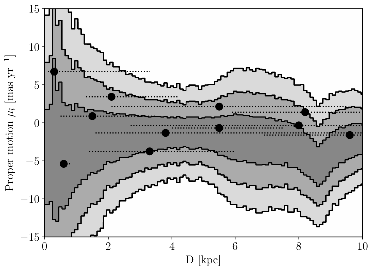
Figure 7.— Same as Figure 5, for the proper motion in latitude along the Galactic plane $\mu_{l}$.

We see the same increase in the dispersion as in Figure 5, when reaching the Galactic bulge. Again, no star is a significant outlier with respect to the theoretical distribution. Without knowing the distances to the targets in Table 5, T18 appears outstanding by its proper motion (total proper motion $\mu$ = 50.5 mas yr^-1), but that corresponds in fact to the short distance to the star, of only 0.6${}^{+0.1}_{-0.2}$ kpc. For that distance, the velocity perpendicular to the line of sight is $v_{\rm perp}$ $\simeq$ 144${}^{+44}_{-48}$ km s^-1, which falls within the range of the model predictions. The same applies to T23, with a proper motion $\mu$ = 7.6 mas yr^-1, at a distance of 0.3${}^{+3.0}_{-0.2}$ kpc only. Table 7 summarizes the main conclusions about the stars within 10 kpc and shows the parameters in relation to the Galaxy model.

K14 note that, according to Blair et al. (1991) and Sollerman et al. (2003), Kepler’s SNR has a systemic radial velocity of -180 km s⁻¹ . As it can be seen from Figure 5, that lies between 2 $\sigma$ and 3 $\sigma$ from the average radial velocity of the stars at $\sim$ 5 kpc from us, in the direction of the SNR. K14 suggest that a possible surviving companion of the SN should have -180 km s^-1 added to the radial velocity component of its orbital motion at the time of the explosion, which would make it more easily identifiable. The systemic velocity of the SNR, however, is that of the exploding WD, which is the sum of the velocity of the center of mass of the system plus the orbital motion of the WD at the time of the explosion. We do not know what the velocity of the center of mass was, and thus we cannot just add those -180 km s^-1 .

7. Results and discussion

Concerning theoretical predictions, we can compare our results with the observational features expected from numerical simulations. All groups that have simulated the impact of the ejecta of a supernova on the companion star (Marietta, Burrows & Frixell 2000; Pakmor et al. 2008; Pan, Ricker & Taam 2012, 2013, Liu et al. 2012, 2013), find that the companion star should have survived the explosion and gain momentum from the disruption of the binary system. Their predictions vary on how luminous would the untied companion be, on how much mass would have lost due to the impact of the supernova ejecta, and on how fast it would rotate and move away from the center of mass of the original system.

Table 7Radial velocities, proper motions, and distances to the 12 stars located at less than 10 kpc

Star	$v_{r}$ (km/s)a	$\mu_{l}$ (mas/yr)	$\mu_{b}$ (mas/yr)	d (kpc)
T03	140.8	1.40$\pm$0.00	-0.38$\pm$0.08	8.2${}^{+20}_{-2.3}$
T04	8.2	-3.75$\pm$0.03	2.41$\pm$0.24	3.3${}^{+2.7}_{-1.9}$
T06	94.4	-0.34$\pm$0.03	-0.75$\pm$0.10	8.0${}^{+17}_{-5.3}$
T08	-84.6	-0.68$\pm$23.70	-0.31$\pm$63.01	5.5${}^{+2.0}_{-1.5}$
T09	-15.8	0.88$\pm$0.07	-0.64$\pm$0.11	1.5${}^{+2.0}_{-1.0}$
T14b	142.3	2.13$\pm$0.00	0.45$\pm$0.09	5.5${}^{+4.0}_{-3.4}$
T15	-23.2	-5.39$\pm$0.00	0.06$\pm$0.09	0.6${}^{+2.2}_{-0.3}$
T18	42.4	32.94$\pm$0.01	36.31$\pm$0.09	0.6${}^{+0.2}_{-0.1}$
T23	50.8	6.73$\pm$0.02	-0.53$\pm$0.06	0.3${}^{+3.0}_{-0.2}$
T24	38.2	-1.33$\pm$0.05	-3.00$\pm$0.09	3.8${}^{+6.8}_{-2.2}$
T29	45.4	3.42$\pm$0.05	3.06$\pm$0.10	2.1${}^{+2.1}_{-0.8}$
T31	-67.5	-1.61$\pm$0.02	2.77$\pm$0.09	9.6${}^{+17}_{-2.7}$

^a The errors in the radial velocities are of 1–2 km/s.

Let us start with the rotational velocities of the post-explosion companions. Liu et al. (2013) did binary population synthesis after performing 3D hydrodynamic simulations of the impact of the ejecta on a main sequence star with different orbital periods and separations from the exploding WD. They obtained the expected distribution of rotational velocities for the surviving companion. It leaves room for a wide range in this parameter, unlike previous assumptions that the post-impacted star should have very high velocities. Pan, Ricker & Taam (2012) also found that angular momentum of the companion would have been lost with the stripped material. In the case of the stars studied in the survey for the companion of SN 1604, all of them have rotational velocities lower than 20 km s^-1. This is not uniquely interpreted as a sign of the absence of companions, though.

Concerning the luminosity discussion, there are some differences in the way the surviving companions from the supernova explosion would be. Podsiadlowski (2003) found that, for a subgiant companion, the object $\sim$ 400 years after the explosion might be significantly overluminous or underluminous relative to its pre-SN luminosity, that depending on the amount of heating and the amount of mass stripped by the impact of the SN ejecta. More recently Shappee, Kochanek & Stanek (2013) have also followed the evolution of luminosity for years after the impact of the ejecta on the companion. The models in which there is mass loss rise in temperature and luminosity peaking at 10⁴ L_⊙ to start cooling and dimming down to 10 L_⊙ some 10⁴ yr after the explosion. Around 500 days after explosion the companion luminosity is 10³ L_⊙. Pan, Ricker & Taam (2012, 2013, 2014) found lower luminosities for the companions than these previous authors. They found luminosities of the order of 10 L_⊙ for the companions, several hundred days after the explosion. It is interesting to see that they predict, for the surviving companions, effective temperatures, T_eff in the range 5000-9000 K. This allows to discard possible candidates below 5000 K in our sample. Only four stars in our sample are at T_eff higher than 5000 K (see Table 4 and Table 7). T04 has 5545 $\pm$ 251 K and log $g$ = 3.8 $\pm$ 0.6. The distance is uncertain but consistent with that of Kepler’s SN: a distance of 3.3${}^{+2.7}_{-1.9}$ kpc. The heliocentric velocity, however, is $v$ = 8.2 km s^-1 and the proper motion, very moderate, $\mu_{l}$ = 3.75 $\pm$ 0.03 mas yr^-1 and $\mu_{b}$ = 7.41 $\pm$ 0.24 mas yr^-1. So, it is within the expectations of the Besançon model. There is only one more target at a distance compatible with Kepler’s SN explosion and $T_{\rm eff}$) higher than 5000K. This target is T23, with a T_eff of 5436 $\pm$ 336 K and log $g$ = 5.3 $\pm$ 1.6, with distance of 0.3${}^{+3.0}_{-0.2}$ kpc. The radial veocity is 50.8 km s^-1 and the proper motion is $\mu_{l}$ = 6.73 $\pm$ 0.02 mas yr^-1 and $\mu_{b}$ = -0.53 $\pm$ 0.06 mas yr^-1.

At a distance compatible with the Kepler SN there are no main sequence stars in our sample (let us recall that we go down to 2.6 L_⊙). There are 4 subgiants and 2 giants at distances compatible with the Kepler distance. Their stellar parameters, radial velocities, rotational velocities and proper motions are within what is expected of a sample field at the Kepler position in our Galaxy.

Target 18 (star A in K14) has a proper motion of $\mu_{l}$ = 32.94 $\pm$ 0.09 mas yr^-1 and $\mu_{b}$ = 36.31 $\pm$ 0.01 mas yr^-1. This is a clear outlier in proper motion and it is crucial to determine its stellar parameters and distance. It turns out that the star is at 0.6${}^{+0.2}_{-0.1}$ kpc only. It is an M star belonging to the main sequence.

Overall, there are no stars showing any peculiarity. All of them have rotational velocities around 10-20 km s^-1 or less, since Giraffe HR15n is not able to measure values lower than that. Their radial velocities are within those expected for field stars.

The predictions by Pan, Ricker & Taam (2012, 2013) were that 400 yrs after the SN Ia explosion, the luminosities of the companion stars would still be 10 times higher than those before receiving the impact of the ejecta of the SN. They have extended those predictions to main sequence (MS) companion masses down to 0.656 M_⊙ and He WDs down to 0.697 M_⊙ (Pan, Ricker & Taam 2014). We have gone below the luminosities predicted for surviving companions of the kind examined by these authors and the predicted T_eff are higher than those found in our sample. They have calculated the post-impact evolution of MS companions and He–WD companions of very low mass at the time of the explosion, and also the post-impact evolution of these companions.

The He WDs at the time of the explosion (Table 1 in Pan, Ricker & Taam 2014) have runaway velocities within the range 490-730 km s^-1, which would correspond, for purely transversal motions at a distance of 5 kpc, to proper motions $\mu$ between 21 and 31 mas yr^-1 or, if assumed to make a 45^o angle with the line of sight, to radial velocities between 350 and 516 km s^-1 and proper motions between 15 and 22 mas yr^-1 Those proper motions would have been detected by the HST astrometry, even for objects fainter than our targets down to m_F814W $\sim$ 22.5 mag.

There are several channels through which WDs could be surviving companions of SN Ia explosions, apart from the He–WDs companion abovementioned. One is dynamically stable accretion on a CO WD from a He-WD or from a lower-mass CO WD (Shen & Schwab 2017). In that case, a He-shell detonation could induce a core explosion (Shen & Bildsten 2014). The mass-donor WD might survive. One salient characteristic of those companions is that, due to their extreme closeness to the exploding WD and to their strong gravitational fields, they should capture part of the radioactive material (⁵⁶Ni) produced by the SN.

Shen & Schwab (2017) study the effects of the decays of ⁵⁶Ni to ⁵⁶Co and of ⁵⁶Co to ⁵⁶Fe, for different masses of captured material by WDs of masses between 0.3 M_⊙ and 0.9 M_⊙. The decays, in the physical conditions prevailing at the surfaces of those WDs, drive persistent winds and produce residual luminosities that, 400 yr after the explosion, are higher than $\sim$10 L_⊙ in all cases (see Fig. 4 in Shen & Schwab 2017). Furthermore, the surviving WDs should be running away from the site of the explosion at velocities $\sim$ 1500-2000 km s^-1. A search for such WD companions has recently been made by Kerzendorf et al. (2018), in the central region of the remnant of SN 1006, with negative result. We have not detected faint hot surviving WDs moving at high speed. We are at larger distance than SN 1006 and the exploration does not go so deep, though (see our completeness discussion).

Another possible channel producing a surviving WD companion is the spin-up, spin-down model (Justham 2011; Di Stefano, Voss & Claeys 2011): the WD, spun up by mass accretion from the companion star, can grown beyond the Chandrasekhar mass; then, when the accretion ceases, it has to lose angular momentum before reaching the point of explosion. During this last time interval, the companion might have evolved past the AGB stage and become a cool WD. The time scale for spin down is hard to be determined theoretically, but Meng & Podsiadlowski (2013) empirically obtain an upper limit of a few 10⁷ yr, for progenitor systems that contain a RG donor and for which circumstellar material has been detected. We must note, however, that the spin-up, spin-down model should mostly produce super-Chandrasekhar explosions, since there is nothing there to tell the system to stop mass transfer just when the WD has reached that mass. In the case of Kepler’s SN, reconstruction of its light curve (Ruiz-Lapuente 2017) clearly indicates that the SN was in no way overluminous.

From all the preceding, we can exclude MS, subgiants, giants, and up to certain extend stars below the solar luminosity.

As an interesting point, no one has yet attempted to calculate how much and for how long the impact of the SN Ia ejecta would affect the luminosity of a WD companion in the spin-up, spin-down case. One can not just assume that the WD would be cold and dim and remain so after the explosion. This has not been proved by any hydrodynamic simulation. It has only been done for closer pairs of WDs, as mentioned above. The typical separation between the two WDs, at the time of the explosion, should be larger that in the cases considered by Pan, Ricker & Taam (2014) and Shen & Schwab (2017), so less radioactive material would be captured and the runaway velocities would also be smaller, but the narrowing of the orbit by the emission of gravitational waves during the cooling stage of the companion WD might not be negligible, and the loss of angular momentum by the system during a likely common-envelope episode preceding the formation of the detached WD-WD system would also have considerably narrowed, previously, the separation between the two objects. We encourage to do these hydrodynamical calculations.

8. Conclusions

We present a study that includes the first detailed stellar parameters: Teff, , log g, v_rot; as well as accurate radial velocities of the stars, and proper motions, using the HST, of possible companions of Kepler’s SN within 20 % of the remnant center. This last part of the research is very important, since one does not know whether the peculiar velocities expected for the surviving companion will mostly be along the line of sight or perpendicular to it. No attempt to measure the proper motions of the stars in the core of Kepler’s SNR had ever been made before.

We have determined luminosities and distances to the candidate companions of Kepler’s SN. Any companion would have luminosities above two times the solar luminosity which is the lowest luminosity of our sample. The radius of our search is 24 arcsecs, that is 20% of the average radius of the SNR. Our stars correspond to stellar parameters and velocities consistent with being from a mixture of stellar populations in the direction of the Kepler SNR.

From our study, we conclude that the single- degenerate scenario is disfavored in the case of Kepler’s supernova. The idea that Kepler’s SN could come from the merging of two stars within a common envelope seems plausible. It would explain why the SN is surrounded by a large circumstellar medium (CSM). The idea of the core-degenerate scenario (Kashi & Soker 2011), that an already existing WD and a degenerate RG core merge inside an AGB envelope, appears very likely in this case.

This analysis makes relevant intensive studies to detect surviving companions in very nearby SNeIa remnants. There are many good cases for study in our Galaxy and in the nearby ones. There are cases in our Galaxy far away enough so that Gaia can not make proper motion estimates, the stars being too dim. The HST plays a key role here. In addition, telescope time in 10m-class telescopes and in the coming generation of large telescopes with high resolution spectrographs is the key to determine the nature of the surviving companions of Type Ia SNe.

As mentioned in the discussion, more hydrodynamical simulations are needed to compare predictions with observational results.

Acknowldegments

Based on observations made with ESO Telescopes at the La Silla Paranal Observatory under programme ID 093.D-0384(A). Based on archival images from the HST programs GO-9731 and GO-12885. The scientific results reported in this article make use of observations by Chandra X-ray Observatory and published previously in cited articles. This research was supported by the Munich Institute for Astro- and Particle Physics (MIAPP) of the DFG cluster of excellence “Origin and Structure of the Universe”. P.R-L is supported by AYA2015-67854-P from the Ministry of Industry, Science and Innovation of Spain and the FEDER funds. J.I.G.H. acknowledges financial support from the Spanish MINECO under the 2013 Ramon y Cajal program MINECO RyC-2013-14875, and also from the Spanish Ministry Project MINECO AYA2014-56359-P. L.G. was supported in part by the US National Science Foundation under Grant AST-1311862. We thank the referee, Wolfgang Kerzendorf, for his very useful report.

References

- (1) Anderson, J. 2002, in van Leeuwen F., Hughes J. D., & Piotto G., eds, ASP Conf. Ser. Vol. 265, Omega Centauri, A Unique Window into Astro- physics (San Francisco, Astron. Soc. Pac.), p. 87
- (2) Anderson, J. 2007, Instrument Science Report ACS 2007-08, STScI, Baltimore
- (3) Anderson, J., & King, I. R. 2006, Instrument Science Report ACS 2006-01, STScI, Baltimore
- (4) Anderson, J., Sarajedini, A., Bedin, L.R., et al. 2008, AJ, 135, 2055A
- (5) Anderson, J., & Bedin, L.R. 2010, Instrument Science Report ACS2010-03, STScI, Baltimore
- (6) Aznar-Siguán, G., García-Berro, E., Lorén-Aguilar, P., Soker, N., & Kashi, A. 2015, MNRAS, 450, 2948
- (7) Bagnulo, S., Jehin, E., Ledoux, C., et al. 2003, Msngr, 114, 10
- (8) Bedin, L.R., Piotto, G., King, I.R., et al. 2003, AJ, 126, 247
- (9) Bedin, L. R., Cassisi, S., Castelli, F., et al. 2005, MNRAS, 357, 1038B
- (10) Bedin, L.R., Anderson, J., Heggie, D.C., et al. 2013, AN, 334, 1062
- (11) Bedin, L.R., Ruiz-Lapuente, P., González Hernández, J.I., et al. 2014, MNRAS, 439, 354
- (12) Bedin, L. R., Salaris, M., Anderson, J., et al, 2015, MNRAS, 448, 1779B
- (13) Bellini, A., & Bedin, L.R. 2009, PASP, 121, 1419
- (14) Bellini, A., Anderson, J., & Bedin, L.R. 2011, PASP, 123, 622
- (15) Blair, W.P., Long, K.S., & Vancura, O. 1991, ApJ, 366, 484
- (16) Canal, R., Méndez, J., & Ruiz-Lapuente, P. 2001, ApJL, 550, L53
- (17) Cassam-Chenaï, G., Decourchelle, A., Ballet, J., et al. 2004, A&A, 414, 545
- (18) Chiotellis, A., Schure, K.M., & Vink, J. 2012, A&A, 537, A139
- (19) Damiani, F., Prisinzano, L., Micela, G., et al. 2014, A&A, 566, A50
- (20) Di Stefano, R., Voss, R., & Claeys, J. S. W. 2011, ApJL, 738, L1
- (21) Edwards, Z. I., Pagnotta, A., & Schaefer, B. E. 2012, ApJL, 747, L19
- (22) Fink, M., Röpke, F.K., Hillebrandt, W., Seitenzahl, I.R., Sim, S. A., & Kromer, M. 2010, A& A, 514, A53
- (23) Freudling, W., Romaniello, M., Bramich, D.M., et al. 2013, arXiV:1311.5411
- (24) González Hernández, J.I., Ruiz-Lapuente, P., Filippenko, A.V., et al. 2009, ApJ, 691, 1
- (25) González Hernández, J.I., Ruiz-Lapuente, P., Tabernero, H.M., et al. 2012, Nature, 489, 533
- (26) Han, Z. 2008, ApJL, 677, L109
- (27) Iben,I., Jr., & Tutukov, A. V. 1984, ApJS, 54, 335
- (28) Jiang, J., Doi, M., Maeda, K., et al. 2017, Nature, 550, 801
- (29) Jackson, R.-J., Jeffries, R.-D., Lewis, J., et al. 2015, A&A, 580, A75
- (30) Justham, S. 2011, ApJL, 730, L34
- (31) Kashi, A., & Soker, N. 2011, MNRAS, 417, 1466
- (32) Katsuda, S., Mori, K., Maeda, K., et al. 2015, ApJ, 808, 49
- (33) Kerzendorf, W.E., Schmidt, B.P.. Asplund, M., et al. 2009, ApJ, 701, 1665
- (34) Kerzendorf, W.E., Schmidt, B.P., Laird, J.B., Podsiadlowski, P., & Bessell, M.S. 2012, ApJ, 759, 7
- (35) Kerzendorf, W.E., Yong, D., Schmidt, B.P., et al. 2013, ApJ, 774, 99
- (36) Kerzendorf, W.E., Childress, M., Scharwächter, J., Do, T., & Schmidt, B.P. 2014, ApJ, 782, 27 (K14)
- (37) Kerzendorf, W. E., Strampelli, G., Shen, K. J. et al. 2018, MNRAS (in press) , arXiV: 1709.06.66
- (38) Li, C.-J., Chu, Y.–H., Gruendl, R., Weisz, D., Pan, K.–C., Points, S.D., Ricker, P., Smith, R.C., & Walter, F.M. 2017, ApJ, 836, 85
- (39) Liu, Z. W., Pakmor, R., Röpcke, F.K. Edelmann, P, Hillebrandt, W., Kerzendorf, W.E., Wang, B., & Han, Z.W. 2013, A&A, 554, 109L
- (40) Livio, M., & Riess, A.G. 2003, ApJ, 594, L93
- (41) Marigo, P., et al. 2017, ApJ, 835, 77
- (42) Meng, X., & Podsiadlowski, P. 2013, ApJL, 778, L35
- (43) Marietta, E., Burrows, A., & Fryell, B. 2000, ApJS, 128, 625
- (44) Nishiyama, S., Nagata, T., & Tamura, M. 2008, ApJ, 680, 1174
- (45) Nomoto, K. 1982, ApJ, 257, 780
- (46) Pagnotta, A, & Schaefer, B. E. 2015, ApJ, 799, 101
- (47) Pakmor, R., Röpcke, F.K., Weiss, A., & Hillebrandt, W. 2008, A&A, 489, 943
- (48) Pan, K.-C., Ricker, P., & Taam, R.E. 2012, ApJ, 750, 151
- (49) Pan, K.-C., Ricker, P., & Taam, R.E. 2013, ApJ, 773, 49
- (50) Pan, K.-C., Ricker, P., & Taam, R.E. 2015, ApJ, 792, 71
- (51) Pasquini, L., Avila, G., Blecha, A., et al. 2002, Messgr, 110, 1
- (52) Podsiadlowski, P. 2003, preprint arXiV: astro-ph-03036660
- (53) Prugniel, Ph., & Soubiran, C. 2001, A&A, 369, 1048
- (54) Reynolds, S.P., Borkowski, K.J., Hwang, U., et al. 2007, ApJL, 66, L135
- (55) Reynoso, E.M., & Goss, W.M. 1999, AJ, 118, 926
- (56) Robin A. C., Haywood M., Créze M., Ojha D. K., & Bienayme, O. 1999, A&A, 305, 125
- (57) Ruiz-Lapuente, P. 2014, NewAR, 62, 15
- (58) Ruiz–Lapuente, P. 2017, ApJ, 842, 112
- (59) Ruiz-Lapuente, P., Comerón, F., Méndez, J., et al. 2004, Nature, 431, 1069
- (60) Sankrit, R., Blair, W.P., Delaney, T., et al. 2005, AdSpR, 35, 1027
- (61) Sankrit, R., Raymond, J.C., Blair, W.P., et al. 2016, ApJ, 817, 36
- (62) Shappee, B.J., Kochanek, C. S., & Stanek, K.Z. 2013, ApJ, 765, 150
- (63) Shen, K. J., & Schwab, J. 2017, ApJ 834, 180
- (64) Shen, K.J, Kasen, D., Broxton, J.M., & Townsley, D. M. 2017, arXiV: 1706.01898
- (65) Sim, S. A. , Fink, M., Kromer, M, Röpke, F.K, Ruiter, A.J., & Hillebrandt, W. 2012. MNRAS, 420, 3003S
- (66) Skrutskie, M.F., Cutri, R.M., Stiening, R., et al. 2006, AJ, 131, 1163
- (67) Soker, N. 2018, Science China Physics, Mechanics & Astronomy, 61, 49502, 10
- (68) Soker, N., Kashi, A., García–Berro, E., Torres, S., & Camacho, J. 2013, MNRAS, 431, 1541
- (69) Soker, N., García–Berro, & Althaus, L.G. 2014, MNRAS, 437, L665
- (70) Sollerman, J., Ghavamian, P., Lundqvist, P., & Smith, R.C. 2003, A&A, 407, 249
- (71) Vink, J. 2008, ApJ, 689. 231
- (72) Vink, J. 2016, in Handbook of Supernovae, ed. by A. W. Alsabti and P. Murdin, arXiV: 161206905
- (73) Wang, B., & Han, Z. 2012, New Astron Revs, 56, 122
- (74) Webbink, R.F. 1984, ApJ, 277, 355
- (75) Whelan, J., & Iben, I.Jr. 1973, ApJ, 186, 1007