Provable Defenses against Adversarial Examples
via the Convex Outer Adversarial Polytope
Abstract
We propose a method to learn deep ReLU-based classifiers that are provably robust against norm-bounded adversarial perturbations on the training data. For previously unseen examples, the approach is guaranteed to detect all adversarial examples, though it may flag some non-adversarial examples as well. The basic idea is to consider a convex outer approximation of the set of activations reachable through a norm-bounded perturbation, and we develop a robust optimization procedure that minimizes the worst case loss over this outer region (via a linear program). Crucially, we show that the dual problem to this linear program can be represented itself as a deep network similar to the backpropagation network, leading to very efficient optimization approaches that produce guaranteed bounds on the robust loss. The end result is that by executing a few more forward and backward passes through a slightly modified version of the original network (though possibly with much larger batch sizes), we can learn a classifier that is provably robust to any norm-bounded adversarial attack. We illustrate the approach on a number of tasks to train classifiers with robust adversarial guarantees (e.g. for MNIST, we produce a convolutional classifier that provably has less than 5.8% test error for any adversarial attack with bounded norm less than ), and code for all experiments is available at http://github.com/locuslab/convex_adversarial.
1 Introduction
Recent work in deep learning has demonstrated the prevalence of adversarial examples (Szegedy et al., 2014; Goodfellow et al., 2015), data points fed to a machine learning algorithm which are visually indistinguishable from “normal” examples, but which are specifically tuned so as to fool or mislead the machine learning system. Recent history in adversarial classification has followed something of a virtual “arms race”: practitioners alternatively design new ways of hardening classifiers against existing attacks, and then a new class of attacks is developed that can penetrate this defense. Distillation (Papernot et al., 2016) was effective at preventing adversarial examples until it was not (Carlini & Wagner, 2017b). There was no need to worry about adversarial examples under “realistic” settings of rotation and scaling (Lu et al., 2017) until there was (Athalye & Sutskever, 2017). Nor does the fact that the adversary lacks full knowledge of the model appear to be a problem: “black-box” attacks are also extremely effective (Papernot et al., 2017). Even detecting the presence of adversarial examples is challenging (Metzen et al., 2017; Carlini & Wagner, 2017a), and attacks are not limited to synthetic examples, having been demonstrated repeatedly on real-world objects (Sharif et al., 2016; Kurakin et al., 2016). Somewhat memorably, many of the adversarial defense papers at the most recent ICLR conference were broken prior to the review period completing (Athalye et al., 2018).
Given the potentially high-stakes nature of many machine learning systems, we feel this situation is untenable: the “cost” of having a classifier be fooled just once is potentially extremely high, and so the attackers are the de-facto “winners” of this current game. Rather, one way to truly harden classifiers against adversarial attacks is to design classifiers that are guaranteed to be robust to adversarial perturbations, even if the attacker is given full knowledge of the classifier. Any weaker attempt of “security through obscurity” could ultimately prove unable to provide a robust classifier.
In this paper, we present a method for training provably robust deep ReLU classifiers, classifiers that are guaranteed to be robust against any norm-bounded adversarial perturbations on the training set. The approach also provides a provable method for detecting any previously unseen adversarial example, with zero false negatives (i.e., the system will flag any adversarial example in the test set, though it may also mistakenly flag some non-adversarial examples). The crux of our approach is to construct a convex outer bound on the so-called “adversarial polytope”, the set of all final-layer activations that can be achieved by applying a norm-bounded perturbation to the input; if we can guarantee that the class prediction of an example does not change within this outer bound, we have a proof that the example could not be adversarial (because the nature of an adversarial example is such that a small perturbation changed the class label). We show how we can efficiently compute and optimize over the “worst case loss” within this convex outer bound, even in the case of deep networks that include relatively large (for verified networks) convolutional layers, and thus learn classifiers that are provably robust to such perturbations. From a technical standpoint, the outer bounds we consider involve a large linear program, but we show how to bound these optimization problems using a formulation that computes a feasible dual solution to this linear program using just a single backward pass through the network (and avoiding any actual linear programming solvers).
Using this approach we obtain, to the best of our knowledge, by far the largest verified networks to date, with provable guarantees of their performance under adversarial perturbations. We evaluate our approach on classification tasks such as human activity recognition, MNIST digit classification, “Fashion MNIST”, and street view housing numbers. In the case of MNIST, for example, we produce a convolutional classifier that provably has less than 5.8% test error for any adversarial attack with bounded norm less than .
2 Background and Related Work
In addition to general work in adversarial attacks and defenses, our work relates most closely to several ongoing thrusts in adversarial examples. First, there is a great deal of ongoing work using exact (combinatorial) solvers to verify properties of neural networks, including robustness to adversarial attacks. These typically employ either Satisfiability Modulo Theories (SMT) solvers (Huang et al., 2017; Katz et al., 2017; Ehlers, 2017; Carlini et al., 2017) or integer programming approaches (Lomuscio & Maganti, 2017; Tjeng & Tedrake, 2017; Cheng et al., 2017). Of particular note is the PLANET solver (Ehlers, 2017), which also uses linear ReLU relaxations, though it employs them just as a sub-step in a larger combinatorial solver. The obvious advantage of these approaches is that they are able to reason about the exact adversarial polytope, but because they are fundamentally combinatorial in nature, it seems prohibitively difficult to scale them even to medium-sized networks such as those we study here. In addition, unlike in the work we present here, the verification procedures are too computationally costly to be integrated easily to a robust training procedure.
The next line of related work are methods for computing tractable bounds on the possible perturbation regions of deep networks. For example, Parseval networks (Cisse et al., 2017) attempt to achieve some degree of adversarial robustness by regularizing the operator norm of the weight matrices (keeping the network non-expansive in the norm); similarly, the work by Peck et al. (2017) shows how to limit the possible layerwise norm expansions in a variety of different layer types. In this work, we study similar “layerwise” bounds, and show that they are typically substantially (by many orders of magnitude) worse than the outer bounds we present.
Finally, there is some very recent work that relates substantially to this paper. Hein & Andriushchenko (2017) provide provable robustness guarantees for perturbations in two-layer networks, though they train their models using a surrogate of their robust bound rather than the exact bound. Sinha et al. (2018) provide a method for achieving certified robustness for perturbations defined by a certain distributional Wasserstein distance. However, it is not clear how to translate these to traditional norm-bounded adversarial models (though, on the other hand, their approach also provides generalization guarantees under proper assumptions, which is not something we address in this paper).
By far the most similar paper to this work is the concurrent work of Raghunathan et al. (2018), who develop a semidefinite programming-based relaxation of the adversarial polytope (also bounded via the dual, which reduces to an eigenvalue problem), and employ this for training a robust classifier. However, their approach applies only to two-layer networks, and only to fully connected networks, whereas our method applies to deep networks with arbitrary linear operator layers such as convolution layers. Likely due to this fact, we are able to significantly outperform their results on medium-sized problems: for example, whereas they attain a guaranteed robustness bound of 35% error on MNIST, we achieve a robust bound of 5.8% error. However, we also note that when we do use the smaller networks they consider, the bounds are complementary (we achieve lower robust test error, but higher traditional test error); this suggests that finding ways to combine the two bounds will be useful as a future direction.
Our work also fundamentally relates to the field of robust optimization (Ben-Tal et al., 2009), the task of solving an optimization problem where some of the problem data is unknown, but belong to a bounded set. Indeed, robust optimization techniques have been used in the context of linear machine learning models (Xu et al., 2009) to create classifiers that are robust to perturbations of the input. This connection was addressed in the original adversarial examples paper (Goodfellow et al., 2015), where it was noted that for linear models, robustness to adversarial examples can be achieved via an norm penalty on the weights within the loss function.111This fact is well-known in robust optimization, and we merely mean that the original paper pointed out this connection. Madry et al. (2017) revisited this connection to robust optimization, and noted that simply solving the (non-convex) min-max formulation of the robust optimization problem works very well in practice to find and then optimize against adversarial examples. Our work can be seen as taking the next step in this connection between adversarial examples and robust optimization. Because we consider a convex relaxation of the adversarial polytope, we can incorporate the theory from convex robust optimization and provide provable bounds on the potential adversarial error and loss of a classifier, using the specific form of dual solutions of the optimization problem in question without relying on any traditional optimization solver.
3 Training Provably Robust Classifiers
This section contains the main methodological contribution of our paper: a method for training deep ReLU networks that are provably robust to norm-bounded perturbations. Our derivation roughly follows three steps: first, we define the adversarial polytope for deep ReLU networks, and present our convex outer bound; second, we show how we can efficiently optimize over this bound by considering the dual problem of the associated linear program, and illustrate how to find solutions to this dual problem using a single modified backward pass in the original network; third, we show how to incrementally compute the necessary elementwise upper and lower activation bounds, using this dual approach. After presenting this algorithm, we then summarize how the method is applied to train provably robust classifiers, and how it can be used to detect potential adversarial attacks on previously unseen examples.
3.1 Outer Bounds on the Adversarial Polytope
In this paper we consider a layer feedforward ReLU-based neural network, given by the equations
| (1) |
with and (the logits input to the classifier). We use to denote the set of all parameters of the network, where represents a linear operator such as matrix multiply or convolution.
We use the set to denote the adversarial polytope, or the set of all final-layer activations attainable by perturbing by some with norm bounded by :222For the sake of concreteness, we will focus on the bound during this exposition, but the method does extend to other norm balls, which we will highlight shortly.
| (2) |
For multi-layer networks, is a non-convex set (it can be represented exactly via an integer program as in (Lomuscio & Maganti, 2017) or via SMT constraints (Katz et al., 2017)), so cannot easily be optimized over.
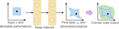
The foundation of our approach will be to construct a convex outer bound on this adversarial polytope, as illustrated in Figure 1. If no point within this outer approximation exists that will change the class prediction of an example, then we are also guaranteed that no point within the true adversarial polytope can change its prediction either, i.e., the point is robust to adversarial attacks. Our eventual approach will be to train a network to optimize the worst case loss over this convex outer bound, effectively applying robust optimization techniques despite non-linearity of the classifier.
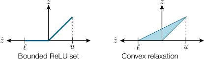
The starting point of our convex outer bound is a linear relaxation of the ReLU activations. Specifically, given known lower and upper bounds , for the pre-ReLU activations, we can replace the ReLU equalities from (1) with their upper convex envelopes,
| (3) |
The procedure is illustrated in Figure 2, and we note that if and are both positive or both negative, the relaxation is exact. The same relaxation at the activation level was used in Ehlers (2017), however as a sub-step for exact (combinatorial) verification of networks, and the method for actually computing the crucial bounds and is different. We denote this outer bound on the adversarial polytope from replacing the ReLU constraints as .
Robustness guarantees via the convex outer adversarial polytope.
We can use this outer bound to provide provable guarantees on the adversarial robustness of a classifier. Given a sample with known label , we can find the point in that minimizes this class and maximizes some alternative target , by solving the optimization problem
| (4) |
where . Importantly, this is a linear program (LP): the objective is linear in the decision variables, and our convex outer approximation consists of just linear equalities and inequalities.333The full explicit form of this LP is given in Appendix A.1. If we solve this LP for all target classes and find that the objective value in all cases is positive (i.e., we cannot make the true class activation lower than the target even in the outer polytope), then we know that no norm-bounded adversarial perturbation of the input could misclassify the example.
We can conduct similar analysis on test examples as well. If the network predicts some class on an example , then we can use the same procedure as above to test whether the network will output any different class for a norm-bounded perturbation. If not, then the example cannot be adversarial, because no input within the norm ball takes on a different class (although of course, the network could still be predicting the wrong class). Although this procedure may incorrectly “flag” some non-adversarial examples, it will have zero false negatives, e.g., there may be a normal example that can still be classified differently due to a norm-bounded perturbation, but all norm-bounded adversarial examples will be detected.
Of course, two major issues remain: 1) although the LP formulation can be solved “efficiently”, actually solving an LP via traditional methods for each example, for each target class, is not tractable; 2) we need a way of computing the crucial and bounds for the linear relaxation. We address these in the following two sections.
3.2 Efficient Optimization via the Dual Network
Because solving an LP with a number of variables equal to the number of activations in the deep network via standard approaches is not practically feasible, the key aspect of our approach lies in our method for very efficiently bounding these solutions. Specifically, we consider the dual problem of the LP above; recall that any feasible dual solution provides a guaranteed lower bound on the solution of the primal. Crucially, we show that the feasible set of the dual problem can itself be expressed as a deep network, and one that is very similar to the standard backprop network. This means that providing a provable lower bound on the primal LP (and hence also a provable bound on the adversarial error), can be done with only a single backward pass through a slightly modified network (assuming for the time being, that we still have known upper and lower bounds for each activation). This is expressed in the following theorem
Theorem 1.
The dual of (4) is of the form
| (5) |
where is equal to
| (6) |
and is a layer feedforward neural network given by the equations
| (7) |
where is shorthand for for all (needed because the objective depends on all terms, not just the first), and where , , and denote the sets of activations in layer where the lower and upper bounds are both negative, both positive, or span zero respectively.
The “dual network” from (7) in fact is almost identical to the backpropagation network, except that for nodes in there is the additional free variable that we can optimize over to improve the objective. In practice, rather than optimizing explicitly over , we choose the fixed, dual feasible solution
| (8) |
This makes the entire backward pass a linear function, and is additionally justified by considerations regarding the conjugate set of the ReLU relaxation (see Appendix A.3 for discussion). Because any solution is still dual feasible, this still provides a lower bound on the primal objective, and one that is reasonably tight in practice.444The tightness of the bound is examined in Appendix B. Thus, in the remainder of this work we simply refer to the dual objective as , implicitly using the above-defined terms.
We also note that norm bounds other than the norm are also possible in this framework: if the input perturbation is bounded within some convex norm, then the only difference in the dual formulation is that the norm on changes to where is the dual norm of . However, because we focus solely on experiments with the norm below, we don’t emphasize this point in the current paper.
3.3 Computing Activation Bounds
Thus far, we have ignored the (critical) issue of how we actually obtain the elementwise lower and upper bounds on the pre-ReLU activations, and . Intuitively, if these bounds are too loose, then the adversary has too much “freedom” in crafting adversarial activations in the later layers that don’t correspond to any actual input. However, because the dual function provides a bound on any linear function of the final-layer coefficients, we can compute for and to obtain lower and upper bounds on these coefficients. For , the backward pass variables (where is now a matrix) are given by
| (9) |
where is a diagonal matrix with entries
| (10) |
We can compute and the corresponding upper bound (which is now a vector) in a layer-by-layer fashion, first generating bounds on , then using these to generate bounds on , etc.
The resulting algorithm, which uses these backward pass variables in matrix form to incrementally build the bounds, is described in Algorithm 1. From here on, the computation of will implicitly assume that we also compute the bounds. Because the full algorithm is somewhat involved, we highlight that there are two dominating costs to the full bound computation: 1) computing a forward pass through the network on an “identity matrix” (i.e., a basis vector for each dimension of the input); and 2) computing a forward pass starting at an intermediate layer, once for each activation in the set (i.e., for each activation where the upper and lower bounds span zero). Direct computation of the bounds requires computing these forward passes explicitly, since they ultimately factor into the nonlinear terms in the objective, and this is admittedly the poorest-scaling aspect of our approach. A number of approaches to scale this to larger-sized inputs is possible, including bottleneck layers earlier in the network, e.g. PCA processing of the images, random projections, or other similar constructs; at the current point, however, this remains as future work. Even without improving scalability, the technique already can be applied to much larger networks than any alternative method to prove robustness in deep networks that we are aware of.
3.4 Efficient Robust Optimization
Using the lower bounds developed in the previous sections, we can develop an efficient optimization approach to training provably robust deep networks. Given a data set , instead of minimizing the loss at these data points, we minimize (our bound on) the worst location (i.e. with the highest loss) in an ball around each , i.e.,
| (11) |
This is a standard robust optimization objective, but prior to this work it was not known how to train these classifiers when is a deep nonlinear network.
We also require that a multi-class loss function have the following property (all of cross-entropy, hinge loss, and zero-one loss have this property):
Property 1.
A multi-class loss function is translationally invariant if for all ,
| (12) |
Under this assumption, we can upper bound the robust optimization problem using our dual problem in Theorem 2, which we prove in Appendix A.4.
Theorem 2.
We denote the upper bound from Theorem 2 as the robust loss. Replacing the summand of (11) with the robust loss results in the following minimization problem
| (14) |
All the network terms, including the upper and lower bound computation, are differentiable, so the whole optimization can be solved with any standard stochastic gradient variant and autodiff toolkit, and the result is a network that (if we achieve low loss) is guaranteed to be robust to adversarial examples.
3.5 Adversarial Guarantees
Although we previously described, informally, the guarantees provided by our bound, we now state them formally. The bound for the robust optimization procedure gives rise to several provable metrics measuring robustness and detection of adversarial attacks, which can be computed for any ReLU based neural network independently from how the network was trained; however, not surprisingly, the bounds are by far the tightest and the most useful in cases where the network was trained explicitly to minimize a robust loss.
Robust error bounds
The upper bound from Theorem 2 functions as a certificate that guarantees robustness around an example (if classified correctly), as described in Corollary 1. The proof is immediate, but included in Appendix A.5.
Corollary 1.
For a data point , label and , if
| (15) |
(this quantity is a vector, so the inequality means that all elements must be greater than zero) then the model is guaranteed to be robust around this data point. Specifically, there does not exist an adversarial example such that and .
We denote the fraction of examples that do not have this certificate as the robust error. Since adversaries can only hope to attack examples without this certificate, the robust error is a provable upper bound on the achievable error by any adversarial attack.
Detecting adversarial examples at test time
The certificate from Theorem 1 can also be modified trivially to detect adversarial examples at test time. Specifically, we replace the bound based upon the true class to a bound based upon just the predicted class . In this case we have the following simple corollary.
Corollary 2.
For a data point , model prediction and , if
| (16) |
then cannot be an adversarial example. Specifically, cannot be a perturbation of a “true” example with , such that the model would correctly classify , but incorrectly classify .
This corollary follows immediately from the fact that the robust bound guarantees no example with norm within of is classified differently from . This approach may classify non-adversarial inputs as potentially adversarial, but it has zero false negatives, in that it will never fail to flag an adversarial example. Given the challenge in even defining adversarial examples in general, this seems to be as strong a guarantee as is currently possible.
-distances to decision boundary
Finally, for each example on a fixed network, we can compute the largest value of for which a certificate of robustness exists, i.e., such that the output provably cannot be flipped within the ball. Such an epsilon gives a lower bound on the distance from the example to the decision boundary (note that the classifier may or may not actually be correct). Specifically, if we find to solve the optimization problem
| (17) |
then we know that must be at least away from the decision boundary in distance, and that this is the largest for which we have a certificate of robustness. The certificate is monotone in , and the problem can be solved using Newton’s method.
4 Experiments
Here we demonstrate the approach on small and medium-scale problems. Although the method does not yet scale to ImageNet-sized classifiers, we do demonstrate the approach on a simple convolutional network applied to several image classification problems, illustrating that the method can apply to approaches beyond very small fully-connected networks (which represent the state of the art for most existing work on neural network verification). Scaling challenges were discussed briefly above, and we highlight them more below. Code for these experiments is available at http://github.com/locuslab/convex_adversarial.
A summary of all the experiments is in Table 1. For all experiments, we report the clean test error, the error achieved by the fast gradient sign method (Goodfellow et al., 2015), the error achieved by the projected gradient descent approach (Madry et al., 2017), and the robust error bound. In all cases, the robust error bound for the robust model is significantly lower than the achievable error rates by PGD under standard training. All experiments were run on a single Titan X GPU. For more experimental details, see Appendix B.
| Problem | Robust | Test error | FGSM error | PGD error | Robust error bound | |
|---|---|---|---|---|---|---|
| MNIST | 0.1 | 1.07% | 50.01% | 81.68% | 100% | |
| MNIST | 0.1 | 1.80% | 3.93% | 4.11% | 5.82% | |
| Fashion-MNIST | 0.1 | 9.36% | 77.98% | 81.85% | 100% | |
| Fashion-MNIST | 0.1 | 21.73% | 31.25% | 31.63% | 34.53% | |
| HAR | 0.05 | 4.95% | 60.57% | 63.82% | 81.56% | |
| HAR | 0.05 | 7.80% | 21.49% | 21.52% | 21.90% | |
| SVHN | 0.01 | 16.01% | 62.21% | 83.43% | 100% | |
| SVHN | 0.01 | 20.38% | 33.28% | 33.74% | 40.67% |
4.1 2D Example
We consider training a robust binary classifier on a 2D input space with randomly generated spread out data points. Specifically, we use a 2-100-100-100-100-2 fully connected network. Note that there is no notion of generalization here; we are just visualizing and evaluating the ability of the learning approach to fit a classification function robustly.
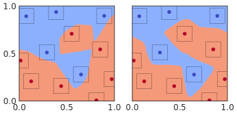
Figure 3 shows the resulting classifiers produced by standard training (left) and robust training via our method (right). As expected, the standard training approach results in points that are classified differently somewhere within their ball of radius (this is exactly an adversarial example for the training set). In contrast, the robust training method is able to attain zero robust error and provides a classifier that is guaranteed to classify all points within the balls correctly.
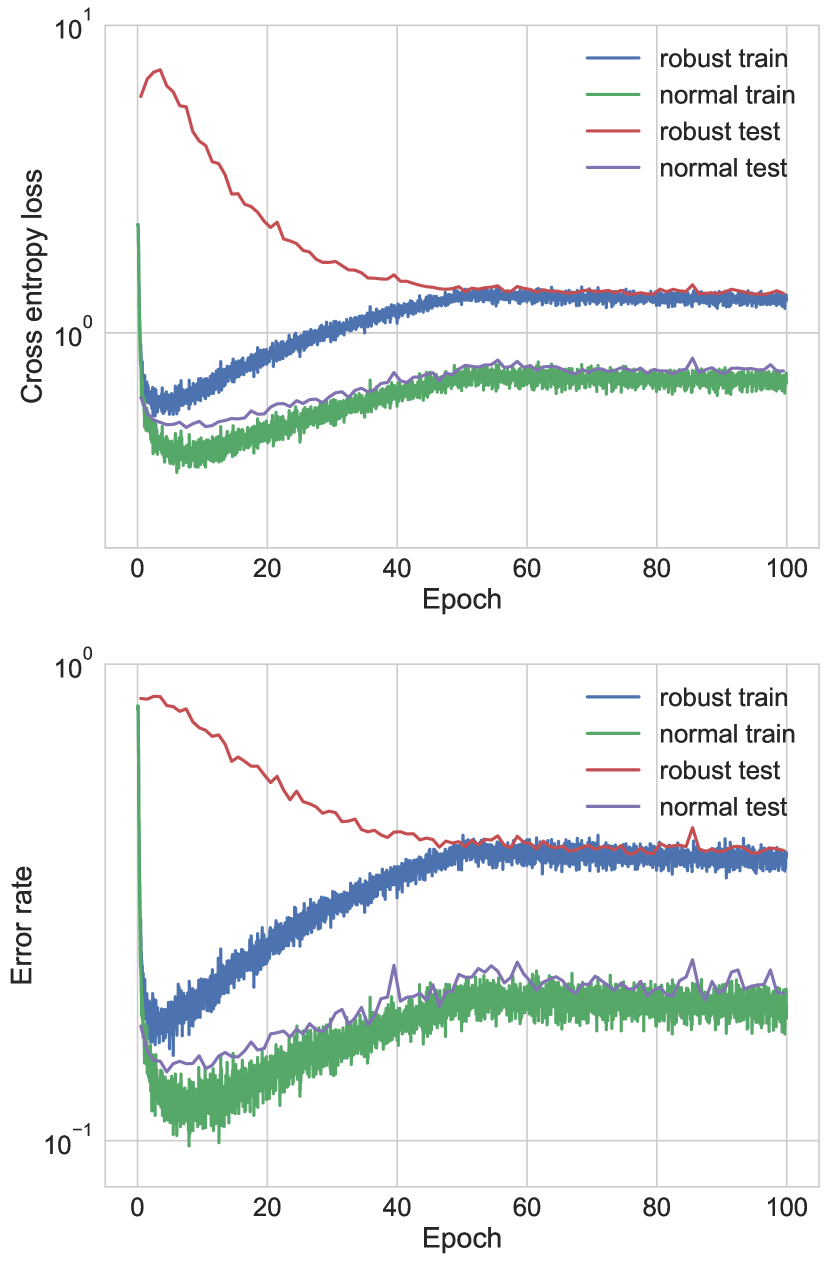
4.2 MNIST
We present results on a provably robust classifier on the MNIST data set. Specifically, we consider a ConvNet architecture that includes two convolutional layers, with 16 and 32 channels (each with a stride of two, to decrease the resolution by half without requiring max pooling layers), and two fully connected layers stepping down to 100 and then 10 (the output dimension) hidden units, with ReLUs following each layer except the last.
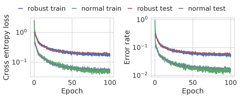
Figure 4 shows the training progress using our procedure with a robust softmax loss function and . As described in Section 3.4, any norm-bounded adversarial technique will be unable to achieve loss or error higher than the robust bound. The final classifier after 100 epochs reaches a test error of 1.80% with a robust test error of 5.82%. For a traditionally-trained classifier (with 1.07% test error) the FGSM approach results in 50.01% error, while PGD results in 81.68% error. On the classifier trained with our method, however, FGSM and PGD only achieve errors of 3.93% and 4.11% respectively (both, naturally, below our bound of 5.82%). These results are summarized in Table 1.
Maximum -distances
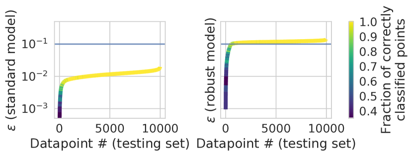
Using Newton’s method with backtracking line search, for each example, we can compute in 5-6 Newton steps the maximum that is robust as described in (17) for both a standard classifier and the robust classifier. Figure 5 shows the maximum values calculated for each testing data point under standard training and robust training. Under standard training, the correctly classified examples have a lower bound of around away from the decision boundary. However, with robust training this value is pushed to 0.1, which is expected since that is the robustness level used to train the model. We also observe that the incorrectly classified examples all tend to be relatively closer to the decision boundary.
4.3 Other Experiments
Fashion-MNIST
We present the results of our robust classifier on the Fashion-MNIST dataset (Xiao et al., 2017), a harder dataset with the same size (in dimension and number of examples) as MNIST (for which input binarization is a reasonable defense). Using the same architecture as in MNIST, for , we achieve a robust error of 34.53%, which is fairly close to the PGD error rate of 31.63% (Table 1). Further experimental details are in Appendix B.3.
HAR
We present results on a human activity recognition dataset (Anguita et al., 2013). Specifically, we consider a fully connected network with one layer of 500 hidden units and , achieving 21.90% robust error.
SVHN
Finally, we present results on SVHN. The goal here is not to achieve state of the art performance on SVHN, but to create a deep convolutional classifier for real world images with provable guarantees. Using the same architecture as in MNIST, for we achieve a robust error bound of 42.09%, with PGD achieving 34.52% error. Further experimental details are in Appendix B.5.
4.4 Discussion
Although these results are relatively small-scale, the somewhat surprising ability here is that by just considering a few more forward/backward passes in a modified network to compute an alternative loss, we can derive guaranteed error bounds for any adversarial attack. While this is by no means state of the art performance on standard benchmarks, this is by far the largest provably verified network we are currently aware of, and 5.8% robust error on MNIST represents reasonable performance given that it is against any adversarial attack strategy bounded in norm, in comparison to the only other robust bound of 35% from Raghunathan et al. (2018).
Scaling to ImageNet-sized classification problems remains a challenging task; the MNIST classifier takes about 5 hours to train for 100 epochs on a single Titan X GPU, which is between two and three orders of magnitude more costly than naive training. But because the approach is not combinatorially more expensive in its complexity, we believe it represents a much more feasible approach than those based upon integer programming or satisfiability, which seem highly unlikely to ever scale to such problems. Thus, we believe the current performance represents a substantial step forward in research on adversarial examples.
5 Conclusion
In this paper, we have presented a method based upon linear programming and duality theory for training classifiers that are provably robust to norm-bounded adversarial attacks. Crucially, instead of solving anything costly, we design an objective equivalent to a few passes through the original network (with larger batch size), that is a guaranteed bound on the robust error and loss of the classifier.
While we feel this is a substantial step forward in defending classifiers, two main directions for improvement exist, the first of which is scalability. Computing the bounds requires sending an identity matrix through the network, which amounts to a sample for every dimension of the input vector (and more at intermediate layers, for each activation with bounds that span zero). For domains like ImageNet, this is completely infeasible, and techniques such as using bottleneck layers, other dual bounds, and random projections are likely necessary. However, unlike many past approaches, this scaling is not fundamentally combinatorial, so has some chance of success even in large networks.
Second, it will be necessary to characterize attacks beyond simple norm bounds. While bounded examples offer a compelling visualization of images that look “identical” to existing examples, this is by no means the only set of possible attacks. For example, the work in Sharif et al. (2016) was able to break face recognition software by using manufactured glasses, which is clearly not bounded in norm, and the work in Engstrom et al. (2017) was able to fool convolutional networks with simple rotations and translations. Thus, a great deal of work remains to understand both the space of adversarial examples that we want classifiers to be robust to, as well as methods for dealing with these likely highly non-convex sets in the input space.
Finally, although our focus in this paper was on adversarial examples and robust classification, the general techniques described here (optimizing over relaxed convex networks, and using a non-convex network representation of the dual problem to derive guaranteed bounds), may find applicability well beyond adversarial examples in deep learning. Many problems that invert neural networks or optimize over latent spaces involve optimization problems that are a function of the neural network inputs or activations, and similar techniques may be brought to bear in these domains as well.
Acknowledgements
This work was supported by a DARPA Young Faculty Award, under grant number N66001-17-1-4036. We thank Frank R. Schmidt for providing helpful comments on an earlier draft of this work.
References
- Anguita et al. (2013) Anguita, D., Ghio, A., Oneto, L., Parra, X., and Reyes-Ortiz, J. L. A public domain dataset for human activity recognition using smartphones. In ESANN, 2013.
- Athalye & Sutskever (2017) Athalye, A. and Sutskever, I. Synthesizing robust adversarial examples. arXiv preprint arXiv:1707.07397, 2017.
- Athalye et al. (2018) Athalye, A., Carlini, N., and Wagner, D. Obfuscated gradients give a false sense of security: Circumventing defenses to adversarial examples. 2018. URL https://arxiv.org/abs/1802.00420.
- Ben-Tal et al. (2009) Ben-Tal, A., El Ghaoui, L., and Nemirovski, A. Robust optimization. Princeton University Press, 2009.
- Carlini & Wagner (2017a) Carlini, N. and Wagner, D. Adversarial examples are not easily detected: Bypassing ten detection methods. In Proceedings of the 10th ACM Workshop on Artificial Intelligence and Security, pp. 3–14. ACM, 2017a.
- Carlini & Wagner (2017b) Carlini, N. and Wagner, D. Towards evaluating the robustness of neural networks. In Security and Privacy (SP), 2017 IEEE Symposium on, pp. 39–57. IEEE, 2017b.
- Carlini et al. (2017) Carlini, N., Katz, G., Barrett, C., and Dill, D. L. Ground-truth adversarial examples. arXiv preprint arXiv:1709.10207, 2017.
- Cheng et al. (2017) Cheng, C.-H., Nührenberg, G., and Ruess, H. Maximum resilience of artificial neural networks. In International Symposium on Automated Technology for Verification and Analysis, pp. 251–268. Springer, 2017.
- Cisse et al. (2017) Cisse, M., Bojanowski, P., Grave, E., Dauphin, Y., and Usunier, N. Parseval networks: Improving robustness to adversarial examples. In International Conference on Machine Learning, pp. 854–863, 2017.
- Ehlers (2017) Ehlers, R. Formal verification of piece-wise linear feed-forward neural networks. In International Symposium on Automated Technology for Verification and Analysis, 2017.
- Engstrom et al. (2017) Engstrom, L., Tsipras, D., Schmidt, L., and Madry, A. A rotation and a translation suffice: Fooling cnns with simple transformations. arXiv preprint arXiv:1712.02779, 2017.
- Goodfellow et al. (2015) Goodfellow, I., Shlens, J., and Szegedy, C. Explaining and harnessing adversarial examples. In International Conference on Learning Representations, 2015. URL http://arxiv.org/abs/1412.6572.
- Hein & Andriushchenko (2017) Hein, M. and Andriushchenko, M. Formal guarantees on the robustness of a classifier against adversarial manipulation. In Advances in Neural Information Processing Systems. 2017.
- Huang et al. (2017) Huang, X., Kwiatkowska, M., Wang, S., and Wu, M. Safety verification of deep neural networks. In International Conference on Computer Aided Verification, pp. 3–29. Springer, 2017.
- Katz et al. (2017) Katz, G., Barrett, C., Dill, D., Julian, K., and Kochenderfer, M. Reluplex: An efficient smt solver for verifying deep neural networks. arXiv preprint arXiv:1702.01135, 2017.
- Kingma & Ba (2015) Kingma, D. and Ba, J. Adam: A method for stochastic optimization. In International Conference on Learning Representations, 2015.
- Kurakin et al. (2016) Kurakin, A., Goodfellow, I., and Bengio, S. Adversarial examples in the physical world. arXiv preprint arXiv:1607.02533, 2016.
- Lomuscio & Maganti (2017) Lomuscio, A. and Maganti, L. An approach to reachability analysis for feed-forward relu neural networks. arXiv preprint arXiv:1706.07351, 2017.
- Lu et al. (2017) Lu, J., Sibai, H., Fabry, E., and Forsyth, D. No need to worry about adversarial examples in object detection in autonomous vehicles. arXiv preprint arXiv:1707.03501, 2017.
- Madry et al. (2017) Madry, A., Makelov, A., Schmidt, L., Tsipras, D., and Vladu, A. Towards deep learning models resistant to adversarial attacks. arXiv preprint arXiv:1706.06083, 2017.
- Metzen et al. (2017) Metzen, J. H., Genewein, T., Fischer, V., and Bischoff, B. On detecting adversarial perturbations. In International Conference on Learning Representations, 2017.
- Papernot et al. (2016) Papernot, N., McDaniel, P., Wu, X., Jha, S., and Swami, A. Distillation as a defense to adversarial perturbations against deep neural networks. In Security and Privacy (SP), 2016 IEEE Symposium on, pp. 582–597. IEEE, 2016.
- Papernot et al. (2017) Papernot, N., McDaniel, P., Goodfellow, I., Jha, S., Celik, Z. B., and Swami, A. Practical black-box attacks against deep learning systems using adversarial examples. In Proceedings of the 2017 ACM Asia Conference on Computer and Communications Security, 2017.
- Peck et al. (2017) Peck, J., Roels, J., Goossens, B., and Saeys, Y. Lower bounds on the robustness to adversarial perturbations. In Advances in Neural Information Processing Systems, pp. 804–813. 2017.
- Raghunathan et al. (2018) Raghunathan, A., Steinhardt, J., and Liang, P. Certified defenses against adversarial examples. In International Conference on Learning Representations, 2018.
- Sharif et al. (2016) Sharif, M., Bhagavatula, S., Bauer, L., and Reiter, M. K. Accessorize to a crime: Real and stealthy attacks on state-of-the-art face recognition. In Proceedings of the 2016 ACM SIGSAC Conference on Computer and Communications Security, pp. 1528–1540. ACM, 2016.
- Sinha et al. (2018) Sinha, A., Namkoong, H., and Duchi, J. Certifiable distributional robustness with principled adversarial training. In International Conference on Learning Representations, 2018.
- Szegedy et al. (2014) Szegedy, C., Zaremba, W., Sutskever, I., Bruna, J., Erhan, D., Goodfellow, I., and Fergus, R. Intriguing properties of neural networks. In International Conference on Learning Representations, 2014. URL http://arxiv.org/abs/1312.6199.
- Tjeng & Tedrake (2017) Tjeng, V. and Tedrake, R. Verifying neural networks with mixed integer programming. CoRR, abs/1711.07356, 2017. URL http://arxiv.org/abs/1711.07356.
- Xiao et al. (2017) Xiao, H., Rasul, K., and Vollgraf, R. Fashion-mnist: a novel image dataset for benchmarking machine learning algorithms. arXiv preprint arXiv:1708.07747, 2017.
- Xu et al. (2009) Xu, H., Caramanis, C., and Mannor, S. Robustness and regularization of support vector machines. Journal of Machine Learning Research, 10(Jul):1485–1510, 2009.
Appendix A Adversarial Polytope
A.1 LP Formulation
Recall (4), which uses a convex outer bound of the adversarial polytope.
| (18) |
With the convex outer bound on the ReLU constraint and the adversarial perturbation on the input, this minimization problem is the following linear program
| (19) |
A.2 Proof of Theorem 1
In this section we derive the dual of the LP in (19), in order to prove Theorem 1, reproduced below:
Theorem.
The dual of (4) is of the form
| (20) |
where
| (21) |
and is a layer feedforward neural network given by the equations
| (22) |
where is shorthand for for all (needed because the objective depends on all terms, not just the first), and where , , and denote the sets of activations in layer where the lower and upper bounds are both negative, both positive, or span zero respectively.
Proof.
In detail, we associate the following dual variables with each of the constraints
| (23) |
where we note that can easily eliminate the dual variables corresponding to the and from the optimization problem, so we don’t define explicit dual variables for these; we also note that , , and are only defined for such that , but we keep the notation as above for simplicity. With these definitions, the dual problem becomes
| (24) | ||||
The key insight we highlight here is that the dual problem can also be written in the form of a deep network, which provides a trivial way to find feasible solutions to the dual problem, which can then be optimized over. Specifically, consider the constraints
| (25) |
Note that the dual variable corresponds to the upper bounds in the convex ReLU relaxation, while and correspond to the lower bounds and respectively; by the complementarity property, we know that at the optimal solution, these variables will be zero if the ReLU constraint is non-tight, or non-zero if the ReLU constraint is tight. Because we cannot have the upper and lower bounds be simultaneously tight (this would imply that the ReLU input would exceed its upper or lower bound otherwise), we know that either or must be zero. This means that at the optimal solution to the dual problem
| (26) |
i.e., the dual variables capture the positive and negative portions of respectively. Combining this with the constraint that
| (27) |
means that
| (28) |
for and for some (this accounts for the fact that we can either put the “weight” of into or , which will or will not be passed to the next ). This is exactly a type of leaky ReLU operation, with a slope in the positive portion of (a term between 0 and 1), and a negative slope anywhere between 0 and 1. Similarly, and more simply, note that and denote the positive and negative portions of , so we can replace these terms with an absolute value in the objective. Finally, we note that although it is possible to have and simultaneously, this corresponds to an activation that is identically zero pre-ReLU (both constraints being tight), and so is expected to be relatively rare. Putting this all together, and using to denote “pre-activation” variables in the dual network, we can write the dual problem in terms of the network
| (29) |
which we will abbreviate as to emphasize the fact that acts as the “input” to the network and are per-layer inputs we can also specify (for only those activations in ), where in this case is shorthand for all the and activations.
The final objective we are seeking to optimize can also be written
| (30) |
∎
A.3 Justification for Choice in
While any choice of results in a lower bound via the dual problem, the specific choice of is also motivated by an alternate derivation of the dual problem from the perspective of general conjugate functions. We can represent the adversarial problem from (2) in the following, general formulation
| (31) | ||||
where represents some input condition and represents some non-linear connection between layers. For example, we can take to get ReLU activations, and take to be the indicator function for an ball with radius to get the adversarial problem in an ball for a ReLU network.
Forming the Lagrangian, we get
| (32) | ||||
Conjugate functions
We can re-express this using conjugate functions defined as
but specifically used as
Plugging this in, we can minimize over each pair independently
| (33) | ||||
Substituting the conjugate functions into the Lagrangian, and letting , we get
| (34) | ||||
This is almost the form of the dual network. The last step is to plug in the indicator function for the outer bound of the ReLU activation (we denote the ReLU polytope) for and derive .
ReLU polytope
Suppose we have a ReLU polytope
| (35) | ||||
So is the indicator for this set, and is its conjugate. We will omit subscripts for brevity, but we can do this case by case elementwise.
-
1.
If then .
Then, . -
2.
If then .
Then, . -
3.
Otherwise . The maximum must occur either on the line over the interval , or at the point (so the maximum must have value at least 0). We proceed to examine this last case.
Let be the set of the third case. Then:
| (36) | ||||
Observe that the second case is always larger than first, so we get a tighter upper bound when . If we plug in and , this condition is equivalent to
Recall that in the LP form, the forward pass in this case was defined by
Then, can be interpreted as the largest choice of which does not increase the bound (because if was any larger, we would enter the second case and add an additional term to the bound).
A.4 Proof of Theorem 2
In this section, we prove Theorem 2, reproduced below:
Theorem.
Proof.
First, we rewrite the problem using the adversarial polytope .
Since for all , we have
| (38) | ||||
where . Since is a monotone loss function, we can upper bound this further by using the element-wise maximum over for , and elementwise-minimum for (note, however, that for , ). Specifically, we bound it as
where, if is the th row of , is defined element-wise as
This is exactly the adversarial problem from (2) (in its maximization form instead of a minimization). Recall that from (6) is a lower bound on (2) (using ).
| (39) |
Multiplying both sides by gives us the following upper bound
Applying this upper bound to , we conclude
Applying this to all elements of gives the final upper bound on the adversarial loss.
∎
A.5 Proof of Corollary 1
In this section, we prove Corollary 1, reproduced below:
Theorem.
For a data point and , if
| (40) |
then the model is guaranteed to be robust around this data point. Specifically, there does not exist an adversarial example such that and .
Proof.
Recall that from (6) is a lower bound on (2). Combining this fact with the certificate in (40), we get that for all ,
Crucially, this means that for every point in the adversarial polytope and for any alternative label , , so the classifier cannot change its output within the adversarial polytope and is robust around . ∎
Appendix B Experimental Details
B.1 2D Example
Problem Generation
We incrementally randomly sample 12 points within the -plane, at each point waiting until we find a sample that is at least away from other points via distance, and assign each point a random label. We then attempt to learn a robust classifier that will correctly classify all points with an ball of .
Parameters
We use the Adam optimizer (Kingma & Ba, 2015) (over the entire batch of samples) with a learning rate of 0.001.


Visualizations of the Convex Outer Adversarial Polytope
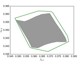
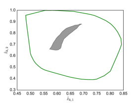
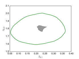
We consider some simple cases of visualizing the outer approximation to the adversarial polytope for random networks in Figure 6. Because the output space is two-dimensional we can easily visualize the polytopes in the output layer, and because the input space is two dimensional, we can easily cover the entire input space densely to enumerate the true adversarial polytope. In this experiment, we initialized the weights of the all layers to be normal and biases normal (due to scaling, the actual absolute value of weights is not particularly important except as it relates to ). Although obviously not too much should be read into these experiments with random networks, the main takeaways are that 1) for “small” , the outer bound is an extremely good approximation to the adversarial polytope; 2) as increases, the bound gets substantially weaker. This is to be expected: for small , the number of elements in will also be relatively small, and thus additional terms that make the bound lose are expected to be relatively small (in the extreme, when no activation can change, the bound will be exact, and the adversarial polytope will be a convex set). However, as gets larger, more activations enter the set , and the available freedom in the convex relaxation of each ReLU increases substantially, making the bound looser. Naturally, the question of interest is how tight this bound is for networks that are actually trained to minimize the robust loss, which we will look at shortly.
Comparison to Naive Layerwise Bounds
One additional point is worth making in regards to the bounds we propose. It would also be possible to achieve a naive “layerwise” bound by iteratively determining absolute allowable ranges for each activation in a network (via a simple norm bound), then for future layers, assuming each activation can vary arbitrarily within this range. This provides a simple iterative formula for computing layer-by-layer absolute bounds on the coefficients, and similar techniques have been used e.g. in Parseval Networks (Cisse et al., 2017) to produce more robust classifiers (albeit there considering perturbations instead of perturbations, which likely are better suited for such an approach). Unfortunately, these naive bounds are extremely loose for multi-layer networks (in the first hidden layer, they naturally match our bounds exactly). For instance, for the adversarial polytope shown in Figure 6 (top left), the actual adversarial polytope is contained within the range
| (41) |
with the convex outer approximation mirroring it rather closely. In contrast, the layerwise bounds produce the bound:
| (42) |
Such bounds are essentially vacuous in our case, which makes sense intuitively. The naive bound has no way to exploit the “tightness” of activations that lie entirely in the positive space, and effectively replaces the convex ReLU approximation with a (larger) box covering the entire space. Thus, such bounds are not of particular use when considering robust classification.
Outer Bound after Training
It is of some interest to see what the true adversarial polytope for the examples in this data set looks like versus the convex approximation, evaluated at the solution of the robust optimization problem. Figure 7 shows one of these figures, highlighting the fact that for the final network weights and choice of epsilon, the outer bound is empirically quite tight in this case. In Appendix B.2 we calculate exactly the gap between the primal problem and the dual bound on the MNIST convolutional model. In Appendix B.4, we will see that when training on the HAR dataset, even for larger , the bound is empirically tight.
B.2 MNIST
Parameters
We use the Adam optimizer (Kingma & Ba, 2015) with a learning rate of 0.001 (the default option) with no additional hyperparameter selection. We use minibatches of size 50 and train for 100 epochs.
scheduling
Depending on the random weight initialization of the network, the optimization process for training a robust MNIST classifier may get stuck and not converge. To improve convergence, it is helpful to start with a smaller value of and slowly increment it over epochs. For MNIST, all random seeds that we observed to not converge for were able to converge when started with and taking uniform steps to in the first half of all epochs (so in this case, 50 epochs).

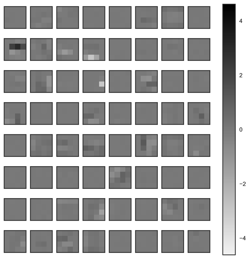
MNIST convolutional filters
Random filters from the two convolutional layers of the MNIST classifier after robust training are plotted in Figure 9. We see a similar story in both layers: they are highly sparse, and some filters have all zero weights.

Activation index counts
We plot histograms to visualize the distributions of pre-activation bounds over examples in Figure 10. We see that in the first layer, examples have on average more than half of all their activations in the set, with a relatively small number of activations in the set. The second layer has significantly more values in the set than in the set, with a comparably small number of activations in the set. The third layer has extremely few activations in the set, with 90% all of the activations in the set. Crucially, we see that in all three layers, the number of activations in the set is small, which benefits the method in two ways: a) it makes the bound tighter (since the bound is tight for activations through the and sets) and b) it makes the bound more computationally efficient to compute (since the last term of (6) is only summed over activations in the set).
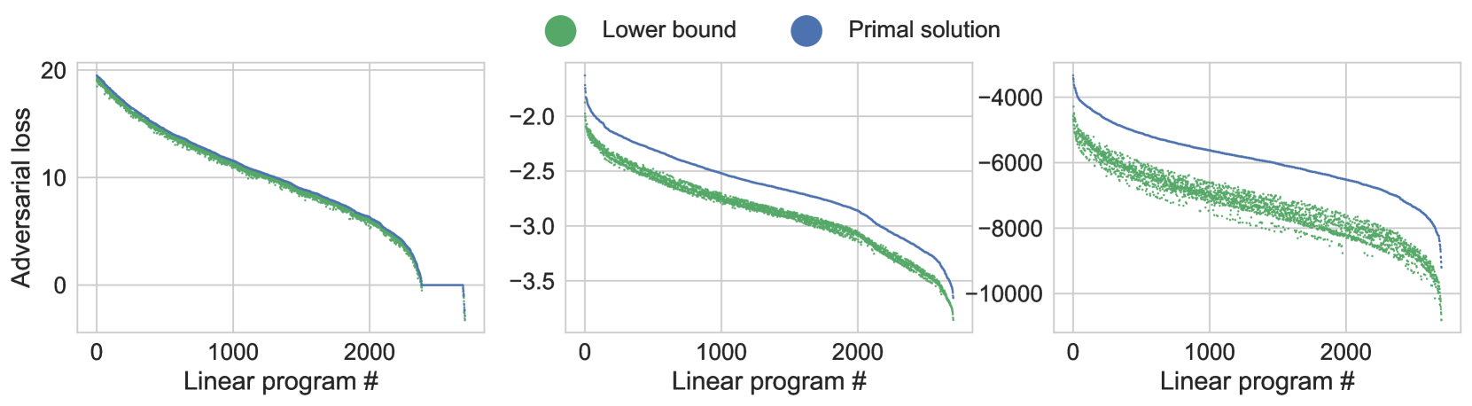
Tightness of bound
We empirically evaluate the tightness of the bound by exactly computing the primal LP and comparing it to the lower bound computed from the dual problem via our method. We find that the bounds, when computed on the robustly trained classifier, are extremely tight, especially when compared to bounds computed for random networks and networks that have been trained under standard training, as can be seen in Figure 11.
B.3 Fashion-MNIST
Parameters
We use exactly the same parameters as for MNIST: Adam optimizer with the default learning rate 0.001, minibatches of size 50, and trained for 100 epochs.
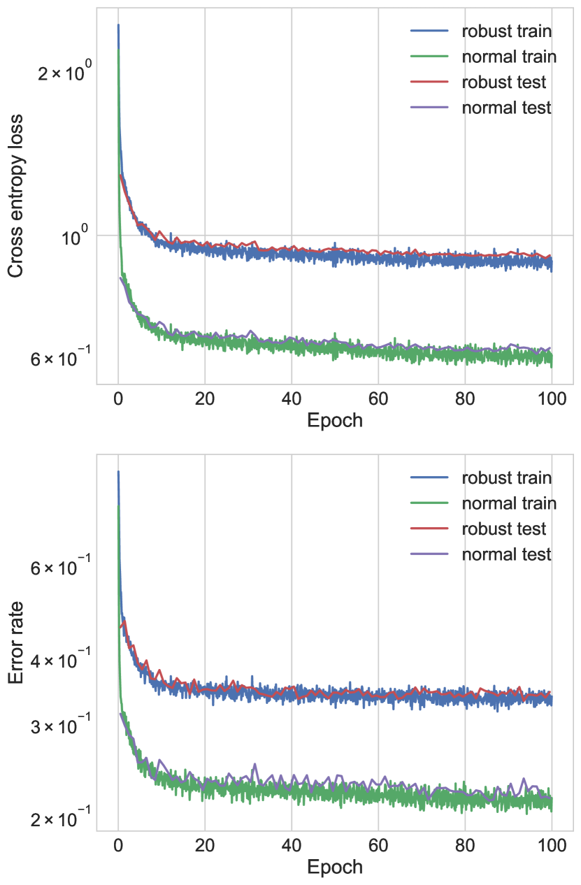
Learning curves
Figure 12 plots the error and loss curves (and their robust variants) of the model over epochs. We observe no overfitting, and suspect that the performance on this problem is limited by model capacity.

B.4 HAR
Parameters
We use the Adam optimizer with a learning rate 0.0001, minibatches of size 50, and trained for 100 epochs.
Learning Curves
Figure 13 plots the error and loss curves (and their robust variants) of the model over epochs. The bottleneck here is likely due to the simplicity of the problem and the difficulty level implied by the value of , as we observed that scaling to more more layers in this setting did not help.
| Test error | FGSM error | Robust bound | |
|---|---|---|---|
| 0.05 | 9.20% | 22.20% | 22.80% |
| 0.1 | 15.74% | 36.62% | 37.09% |
| 0.25 | 47.66% | 64.24% | 64.47% |
| 0.5 | 47.08% | 67.32% | 67.86% |
| 1 | 81.80% | 81.80% | 81.80% |
Tightness of bound with increasing
Earlier, we observed that on random networks, the bound gets progressively looser with increasing in Figure 6. In contrast, we find that even if we vary the value of , after robust training on the HAR dataset with a single hidden layer, the bound still stays quite tight, as seen in Table 2. As expected, training a robust model with larger results in a less accurate model since the adversarial problem is more difficult (and potentially impossible to solve for some data points), however the key point is that the robust bounds are extremely close to the achievable error rate by FGSM, implying that in this case, the bound is tight.
B.5 SVHN
Parameters
We use the Adam optimizer with the default learning rate 0.001, minibatches of size 20, and trained for 100 epochs. We used an schedule which took uniform steps from to over the first 50 epochs.
Learning Curves
Note that the robust testing curve is the only curve calculated with throughout all 100 epochs. The robust training curve was computed with the scheduled value of at each epoch. We see that all metrics calculated with the scheduled value steadily increase after the first few epochs until the desired is reached. On the other hand, the robust testing metrics for steadily decrease until the desired is reached. Since the error rate here increases with , it suggests that for the given model capacity, the robust training cannot achieve better performance on SVHN, and a larger model is needed.