Strong lensing modeling in galaxy clusters as a promising method to test cosmography I. Parametric dark energy models

Abstract

In this paper we probe five cosmological models for which the dark energy equation of state parameter, $w(z)$, is parameterized as a function of redshift using strong lensing data in the galaxy cluster Abell 1689. We constrain the parameters of the $w(z)$ functions by reconstructing the lens model under each one of these cosmologies with strong lensing measurements from two galaxy clusters: Abell 1689 and a mock cluster, Ares, from the Hubble Frontier Fields Comparison Challenge, to validate our methodology. To quantify how the cosmological constraints are biased due to systematic effects in the strong lensing modeling, we carry out three runs considering the following uncertainties for the multiple images positions: $0.25\arcsec$, $0.5\arcsec$, and $1.0\arcsec$. With Ares, we find that larger errors decrease the systematic bias on the estimated cosmological parameters. With real data, our strong-lensing constraints on $w(z)$ are consistent those derived from other cosmological probes. We confirm that strong lensing cosmography with galaxy clusters is a promising method to constrain $w(z)$ parameterizations. A better understanding of galaxy clusters and their environment is however needed to improve the SL modeling and hence to estimate stringent cosmological parameters in alternatives cosmologies.

1 Introduction

Current cosmological observations provide strong evidence that the expansion of the Universe is accelerating (Riess et al., 1998; Perlmutter et al., 1999; Planck Collaboration et al., 2016b). The source of this cosmic acceleration is a big puzzle in modern cosmology and two hypothesis have been proposed to explain it: either to postulate the existence of a dark energy component or to modify the gravity laws (Joyce et al., 2016). Among the first kind of models, the cosmological constant, which is commonly associated to the quantum vacuum energy, has been established as the preferred candidate to the nature of dark energy by several cosmological measurements (e.g. Planck Collaboration et al., 2016a). By definition, the equation of state (EoS, hereafter) parameter of the cosmological constant is $w=-1$. Nonetheless, when a general constant equation of state is considered, the data constrain $w=-1.019^{+0.075}_{-0.080}$ (Planck Collaboration et al., 2016b, see also Neveu et al., 2017), which is consistent with the cosmological constant. In spite of this consistency, the theoretical expected value of the vacuum energy differs in many orders of magnitude from the observed one. In addition, the coincidence problem, i.e. the similitude seen at the current time between the dark matter energy density and that of DE, remains unsolved (Zeldovich, 1968; Weinberg, 1989). Several dark energy (DE, hereafter) models, as for instance, dynamical dark energy or interacting dark energy (Copeland et al., 2006; Li et al., 2011), are also in agreement with the data and they can satisfactorily describe the late-time acceleration of the Universe in a similar way as the cosmological constant does (Ferreira et al., 2017; Salvatelli et al., 2014; Zhao et al., 2017). Therefore, to distinguish which cosmological model is the more suitable to the nature of dark energy, we need to put tight constraints on their parameters. A standard way to estimate these parameters is to perform a Bayesian analysis using classic cosmological probes, i.e. to fit the distance modulus of type Ia distant supernovae (SNIa), Hubble parameter measurements, baryon acoustic oscillation (BAO) signal, and the acoustic peaks of the cosmic microwave background (CMB) radiation (Davis, 2014; Mortonson et al., 2014). Although these tests are widely used to constrain cosmological models, they could yield to biased estimations because either the data or the test fitting formulas are derived assuming an underlying standard cosmology $\Lambda\mathrm{CDM}$ (i.e. the cosmological constant as dark energy plus cold dark matter). Thus, it is essential to construct methods to estimate the parameters of alternative cosmologies without assuming any fiducial cosmology. One novel technique is to use strong lensing measurements in galaxy clusters.

Strong gravitational lensing (SL, hereafter) offers a unique and independent opportunity to constrain dark energy features without prior assumptions on the fiducial cosmology. Link & Pierce (1998) introduced a new approach by leveraging the cosmological sensitivity of the angular size-redshift relation when multiples imaged systems (over a broad range of redshift) are produced by strong lensing clusters. This technique was later on extended to more complex simulated clusters by Golse et al. (2002) and to real clusters such as Abell 2218 (see Soucail et al., 2004), showing that SL cosmography is a promising geometrical cosmological test. Jullo et al. (2010) used an improved technique which simultaneously reconstructed the mass distribution of Abell 1689 (A1689, hereafter), adopting a parametric lens modeling, and constrained the parameters of a $w$CDM cosmology. For the first time, the authors obtained competitive constraints on the equation of state parameter and found that, by combining their results with other probes, they improved the DE EoS estimation by $\sim 30\%$. Following the same method, Caminha et al. (2016) recently used the SL measurements in Abell S1063 with the pre-Frontier Fields data to constrain cosmological parameters for three different $\Lambda\mathrm{CDM}$ models. They pointed out the importance of estimating the parameters using multiply lensed sources with a wide range of redshifts. The authors also showed that the lack of spectroscopic measurements or the use of inaccurate photometric redshifts leads to a biased estimation of the cosmological parameters. Magaña et al. (2015) exploited this technique too, but using alternative cosmologies. They used A1689 strong lensing measurements to constrain four dark energy models: Chevallier-Polarski-Linder (CPL), Interacting Dark Energy (IDE), Ricci Holographic Dark Energy (RHDE), and Modified Polytropic Cardassian (MPC) . They found that the SL method provides CPL constraints in good agreement with those obtained with the SNe Ia, BAO and CMB data. In addition, the IDE and RHDE constraints derived from SL are similar to those estimated with other tests. Nevertheless, the IDE constraints are consistent with the complementary bounds only if an increase in the image-position error (five times the one previously used by Jullo et al., 2010) is considered in the lens modeling. They confirmed that, to avoid misleading DE bounds, it is important to consider larger positional uncertainties for the multiple images; which could be associated with systematic errors.

Indeed, SL has various known sources of systematic errors. D’Aloisio & Natarajan (2011), using simulations of cluster lenses, showed that the observational errors (for space-based images) are an order of magnitude smaller that the modeling errors. Furthermore, line-of-sight (LOS) structures can introduce a systematic error in the strong lensing modeling (e.g. Bayliss et al., 2014; Giocoli et al., 2016; Host, 2012; Jaroszynski & Kostrzewa-Rutkowska, 2014; McCully et al., 2014) of up to $\sim 1.4\arcsec$ on the position of multiple images (Zitrin et al., 2015). Even distant massive structures in the lens plane have a significant impact on the position of multiple images (Tu et al., 2008; Limousin et al., 2010). Harvey et al. (2016), by analyzing the Frontier Field cluster MACSJ0416 ($z=0.397$), estimated an error of $\sim 0.5\arcsec$ on the position of the multiple images when assuming that light traces mass in the SL modeling. However, few studies have investigated their impact on the retrieval of cosmological parameters (McCully et al., 2017; Acebron et al., 2017).

In this paper, we are interested in quantifying the uncertainties in the estimation of cosmological parameters induced by different positional errors of the multiple images. To this end, we analyze the strong lensing effect in the galaxy cluster A1689, as well as in a mock galaxy cluster at $z=0.5$ generated in a flat ${\Lambda\mathrm{CDM}}$ cosmology. Because in the CLP case it is possible to obtain tight constraints on its parameters (see Magaña et al., 2015) using the SL methodology proposed by Jullo et al. (2010), in this work we consider popular CPL-like models in which the EoS of dark energy is parametrized as function of redshift.

The paper is organized as follows: in the next section, §2, we introduce the cosmological framework and the parametric dark energy models. In section §3 we describe the SL data and methodology used to constrain the cosmological parameters of the DE models. In section §4 we present and discuss the results. Finally, we provide our conclusions in section §5.

2 Cosmological framework and parametric dark energy models

For a homogeneous, isotropic, and flat Friedmann-Lemaître-Robertson-Walker (FLRW) cosmology, the expansion rate of the Universe is governed by the Friedmann equation:

$$H^{2}(z)\equiv\frac{8\pi G}{3}\sum_{i}\rho_{i}(z),$$ (1)

where $H\equiv\dot{a}/a$ is the Hubble parameter, $a$ is the scale factor of the Universe, and $\rho_{i}$ denotes the energy density for each component in the Universe. We consider cold dark matter ($m$) and radiation ($r$) components whose dynamics are described by a perfect fluid with EoS $w_{m}=0$ and $w_{r}=1/3$, respectively. In addition, we also consider a dynamical dark energy ($de$) whose EoS is parameterized by a $w(z)$ function. In terms of the present values of the density parameters, $\Omega_{i}\equiv 8\pi G\rho_{i}/3H(z)^{2}$, for each component, the Eq. 1 reads as:

$$E^{2}(z)=\Omega_{m}(1+z)^{3}+\Omega_{r}(1+z)^{4}+\Omega_{de}f_{de}(z),\quad$$ (2)

where $E(z)=H(z)/H_{0}$ is the dimensionless Hubble parameter, $\Omega_{r}=2.469\times 10^{-5}h^{-2}(1+0.2271N_{eff})$, with $h=H_{0}/100\mathrm{kms}^{-1}\mathrm{Mpc}^{-1}$, $N_{eff}=3.04$ is the standard number of relativistic species (Komatsu et al., 2011), and $\Omega_{de}$ can be expressed as $\Omega_{de}=1-\Omega_{m}-\Omega_{r}$. The function $f_{de}(z)$ is defined as:

$$f_{de}(z)\equiv\frac{\rho_{de}(z)}{\rho_{de}(0)}=\mathrm{exp}\left(3\int^{z}_{0}\frac{1+w(z)}{1+z}\mathrm{dz}\right).$$ (3)

Notice that, by introducing a $w(z)$ functional form in the integral of the Eq. (3), we can obtain an analytical expression for $f_{de}(z)$, and hence for $E(z)$.

Besides, to test whether the constraints for each parametric DE model result in a late cosmic acceleration, we examine the deceleration parameter q(z) defined as:

$$q(z)=-\frac{\ddot{a}(z)a(z)}{\dot{a}^{2}(z)}.$$ (4)

Using Eq. (2), we obtain:

$$q(z)=\frac{(1+z)}{E(z)}\frac{dE(z)}{dz}-1,$$ (5)

which expresses the deceleration parameter in terms of the dimensionless Hubble parameter.

2.1 Parametric dark energy models

One alternative to the cosmological constant is to consider a dark energy component which admits a time-dependent EoS. An effective and simple way to study dynamical dark energy models is to assume a phenomenological parameterization of the EoS (Lazkoz et al., 2005; Pantazis et al., 2016). Commonly, this EoS is biparametric and it depends on the scale factor of redshift. The most popular ansatz, denoted Chevallier-Polarski-Linder parameterization, (introduced and revisited by Chevallier & Polarski, 2001; Linder, 2003, respectively) is $w(z)=w_{0}+w_{1}z/(1+z)$, where $w_{0}$ is the present value of the equation of state and $w_{1}=dw(z)/dz|_{z=0}$. In this paper we study five CPL-like EoS parameterizations (see Magaña et al., 2014; Wang et al., 2016, for details), in the following, we briefly introduce the functional form of these parameterizations.

• Jassal-Bagla-Padmanabhan (JBP).- Jassal et al. (2005b, a) proposed that the dark energy EoS is parameterized by the function

  $$w(z)=w_{0}+w_{1}\frac{z}{\left(1+z\right)^{2}},$$ (6)

  which allows rapid variations at low $z$. The DE has the same EoS at the present epoch and at high redshift, i.e., $w(\infty)=w_{0}$. By substituting the Eq. (6) in Eq. (3) we obtain:

  $$f_{de}(z)=(1+z)^{3(1+w_{0})}\mathrm{exp}\left[\frac{3}{2}\frac{w_{1}z^{2}}{(1+z)^{2}}\right].$$ (7)

• Barbosa-Alcaniz (BA).- Barboza & Alcaniz (2008) considered a parametric EoS for the dark energy component given by:

  $$w(z)=w_{0}+w_{1}\frac{z(1+z)}{1+z^{2}}.$$ (8)

  This ansatz behaves linearly at low redshifts as $w_{0}+w_{1}$, and $w\rightarrow w_{0}+w_{1}z$ when $z\rightarrow\infty$. In addition, $w(z)$ is well-behaved in all epochs of the Universe, for instance, the DE dynamics in the future, at $z=-1$, can be investigated without dealing with a divergence. Solving the integral in Eq. (3) and using Eq. (8) results in:

  $$f_{de}(z)=(1+z)^{3(1+w_{0})}(1+z^{2})^{\frac{3}{2}w_{1}}.$$ (9)

• Feng-Shen-Li-Li (FSLL, Feng et al., 2012) suggested two dark energy EoS parameterizations given by:

  $$w(z)=w_{0}+w_{1}\frac{z}{1+z^{2}},\qquad\textrm{FSLLI}$$ (10)

  $$w(z)=w_{0}+w_{1}\frac{z^{2}}{1+z^{2}}\qquad\textrm{FSLLII}.$$ (11)

  Both functions have the advantage of being divergence-free throughout the entire cosmic evolution, even at $z=-1$. At low redshifts, $w(z)$ behaves as $w_{0}+w_{1}z$ and $w_{0}+w_{1}z^{2}$ for FSLLI and FSLLII respectively. In addition, when $z\rightarrow\infty$, the EoS has the same value, $w_{0}$, as the present epoch for FSLLI and $w_{0}+w_{1}$ for FSLLII. Using Eqs. (10)-(11) to solve Eq. (3) leads to:

  $$f_{de\pm}(z)=(1+z)^{3(1+w_{0})}\mathrm{exp}\left[\pm\frac{3w_{1}}{2}\mathrm{arctan(z)}\right]\left(1+z^{2}\right)^{\frac{3}{4}w_{1}}\left(1+z\right)^{\mp\frac{3}{2}w_{1}},$$ (12)

  where $f_{+}$ and $f_{-}$ correspond to FSLLI and FSLLII respectively.

• Sendra-Lazkoz (SeLa, Sendra & Lazkoz, 2012) improved the CPL parameterization, whose $w_{0}-w_{1}$ parameters are highly correlated and $w_{1}$ is poorly constrained by the observational data, introducing new polynomial parameterizations. They are constructed to reduce the parameter correlation, so they can be better constrained by the observations at low redshifts. One of these parameterizations is given by:

  $$w(z)=-1+c_{1}\left(\frac{1+2z}{1+z}\right)+c_{2}\left(\frac{1+2z}{1+z}\right)^{2},\\$$ (13)

  where the constants are defined as $c_{1}=(16w_{0}-9w_{0.5}+7)/4$, and $c_{2}=-3w_{0}+(9w_{0.5}-3)/4$, and $w_{0.5}$ is the value of the EoS at $z=0.5$. This $w(z)$ function is well-behaved at higher redshifts as $(-1-8w_{0}+9w_{0.5})/2$. By the substitution of Eq. (13) into Eq. (3), we obtain:

  $$f_{de}(z)=(1+z)^{\frac{3}{2}(1-8w_{0}+9w_{0.5})}\mathrm{exp}\left[\frac{3z\left\{w_{0}(52z+40)-9w_{0.5}(5z+4)+7z+4\right\}}{8(1+z)^{2}}\right].$$ (14)

By replacing the $f_{de}(z)$ functions in Eq. (1), we obtain an analytical $E(z)$ function for each parametric $w(z)$, which will be used in the following sections to estimate the EoS parameters. Our main purpose is to examine the quality of the $w(z)$ constraints extracted from the SL modeling when different image-position errors are considered.

3 Methodology

3.1 Strong lensing as a cosmological probe

The gravitational lensing effect is produced when the light-beam of a background source is deflected by a gravitational lens, i.e. a mass distribution between the source and the observer. We refer to the strong lensing regime when several rings, arcs or multiples images are observed as a result of the distortion and deflection of the light from a source by a lens. These strong lensing observables offer a powerful and useful tool to not only infer the total matter distribution in astrophysical systems (Jauzac et al., 2014; Monna et al., 2017), but also to provide insights on the total content of the Universe, dark matter and dark energy properties (Golse et al., 2002; Soucail et al., 2004; Jullo et al., 2010; Caminha et al., 2016; Magaña et al., 2015). Here, we use strong lensing measurements in galaxy clusters to constrain the equation of state of parametric dark energy models.

Since the strong lensing features depend on the dynamics of the Universe via the angular diameter distance between the source, lens and observer, it can be used as a geometric cosmological probe. For any underlying cosmology, the angular diameter distance ratios for two images from different sources defines the ’family ratio’ (see Jullo et al., 2010, for a detailed discussion):

$$\Xi(z_{1},z_{s1},z_{s2},\mathbf{\Theta})=\frac{D(z_{1},z_{s1})}{D(0,z_{s1})}\frac{D(0,z_{s2})}{D(z_{1},z_{s2})},$$ (15)

where $\mathbf{\Theta}$ is the vector of cosmological parameters to be fitted, $z_{1}$ is the lens redshift, $z_{s1}$ and $z_{s2}$ are the two source redshifts, and $D(z_{i},z_{f})$ is the angular diameter distance calculated as:

$$D(z_{i},z_{f})=\frac{r(z_{i},z_{f})}{(1+z_{f})},$$ (16)

where $r(z_{i},z_{f})$, the comoving distance of a source at redshift $z_{f}$ measured by an observer at redshift $z_{i}$, is given by

$$r(z_{i},z_{f})=\frac{c}{H_{0}}\int_{z_{i}}^{z_{f}}\frac{dz^{\prime}}{E(z^{\prime})}.$$ (17)

Notice that the underlying cosmology in the lens modeling is selected by introducing the $E(z)$ function in the Eq. (17). For the parametric DE models, these functions are analytical and $\mathbf{\Theta}=\{\Omega_{m},w_{0},w_{1}\}$ ($w_{0.5}$ for the SeLa parameterization) is the free parameter vector.

3.2 Lensing modeling

To constrain the parameters of the DE models presented in 2.1, we use the SL measurements in two galaxy clusters: a real one, Abell 1689, and a simulated one, Ares from the Frontier Fields Comparison Challenge (Meneghetti et al., 2016).
We performed the SL modeling using the public software LENSTOOL (Kneib et al., 1996; Jullo et al., 2007) in which the DE cosmological models described in 2.1 were implemented. LENSTOOL is a ray-tracing code with a Bayesian Markov Chain Monte-Carlo sampler which optimizes the model parameters using the positions of the multiply imaged systems. The matter distribution in clusters is modeled in a parametric way and the optimization is performed in the image plane for Abell 1689 as it is more precise (this is different from the analysis by Jullo et al., 2010; Magaña et al., 2015, where the optimization was performed in the source plane). For Ares, the optimization was realized in the source plane as it is a more complex cluster (more images and cluster members) and this procedure is more computationally efficient. We checked that results in the image plane were similar for a subset of calculations.

For both Abell 1689 and Ares, each potential (either large or galaxy-scale) is parametrized with the Pseudo Isothermal Elliptical Mass Distribution profile (hereafter PIEMD, Kassiola & Kovner, 1993; Elíasdóttir et al., 2007). The density distribution of this profile is given by:

$$\centering\rho(r)=\frac{\rho_{0}}{(1+\frac{r^{2}}{{r_{core}}^{2}})(1+\frac{r^{2}}{{r_{cut}}^{2}})}\mathrm{,}\@add@centering$$ (18)

with a central density $\rho_{0}$, a core radius $r_{core}$ and a truncation radius $r_{cut}$. This profile is characterized by two changes in the density slope: it behaves as an isothermal profile within the transition region but the density falls as $\rho\propto r^{-4}$ at large radii. In LENSTOOL, it has the following free parameters: the coordinates x, y; the ellipticity, e; angle position, $\theta$; core and cut radii, $r_{core}$ and $r_{cut}$ and a velocity dispersion, $\sigma$. Both clusters were modeled in the same way regardless of the considered DE cosmological model.

Abell 1689.- a massive cluster at redshift $z=0.18$, is one of the most studied strong lenses (see e.g., Limousin et al., 2007, 2013; Umetsu et al., 2015; Diego et al., 2015, and references therein). The first SL modeling was performed by Miralda-Escude & Babul (1995) which already required a bi-modal mass distribution for the cluster. It is one of the most X-ray luminous clusters and has a large Einstein radii, $\sim 45\arcsec$. A1689 is still the target of recent observations, using MUSE data with which Bina et al. (2016) confirmed or spectroscopically identified new multiples images as well as cluster members.

We refer the reader to Jullo et al. (2010) for a detailed discussion of the modeling of A1689, where a SL parametric model was used to constrain the DE EoS. As we follow-up their approach, we give here a quick overview. Abell 1689 was modeled using the SL features in the deep HST observations and extensive ground-based spectroscopic follow-up. The mass distribution was represented as bi-modal, with one central and dominant large-scale potential harboring a brightest central cluster galaxy (BCG) in its centre. The second large-scale potential was situated in the north-east. Jullo et al. (2010) used 58 cluster galaxies (with $m_{K}<18.11$) in the modeling and followed the standard scaling relations. In this work we consider the same catalog as in Jullo et al. (2010), including 28 images from 12 families, all with measured spectroscopic redshifts, spanning a range of 1.15 $<z_{S}<$ 4.86.

Ares.- a mock galaxy cluster at $z=0.5$, generated in a flat ${\Lambda\mathrm{CDM}}$ cosmological model with a matter density parameter $\mathrm{\Omega_{m}}=0.272$. We model Ares considering all multiple images (242 from 85 sources), all with assumed known spectroscopic redshifts spanning a wide range ($0.91<z_{S}<6.0$). Cluster members are taken from the given simulated catalogue up to a magnitude of $m_{F160W}<22.0$ mag (representing $>90\%$ of the total cluster luminosity). Ares is part of an archive of mock clusters which reproduce the characteristics of the Frontier Fields observations (the FF-SIMS Challenge, Meneghetti et al., 2016). It was part of a challenge among the strong lensing community to perform, first a blind reconstruction of the mass distribution of the cluster, and then to improve the models after the unblinding of the true mass distribution. The conclusions of this challenge were primarily used to calibrate different modeling techniques. Ares is a semi-analytical cluster created with MOKA by Giocoli et al. (2012). This simulated cluster, a bimodal and realistic cluster, is built with three components: two smooth dark matter triaxial haloes, two bright central cluster galaxies (BCGs) and a large number of sub-haloes. Dark matter sub-haloes are populated using a Halo Occupation Distribution technique (HOD) and stellar and B-band luminosities are given for all galaxies according to the mass of their sub-halo as in Wang et al. (2006).
We have modeled Ares as two large-scale potentials and two potentials for the BCGs, whose coordinates are fixed as well as the ones for the large-scale potentials (see Figure 1 in Acebron et al., 2017). Both components have been parametrized with the PIEMD density profile and corresponds to the model PIEMD - PIEMD in Acebron et al. (2017). The modeling also includes cluster galaxies with $m_{F160W}<22$ mag (being a more complex cluster, computing time is reduced by introducing a magnitude cut representing $>90\%$ of the total cluster luminosity) with masses scaling with luminosity (see Limousin et al., 2005, for further details). Three massive cluster galaxies close to multiple images (see Figure 1 in Acebron et al., 2017) were more carefully modeled (i.e their parameters deviate from the scaling relations). All multiple images provided were taken into account in the modeling, resulting in an average positional accuracy of $0.66\arcsec$ and giving tight constraints on the $\Omega_{M}-w$ space parameter considering a flat ${\Lambda\mathrm{CDM}}$ cosmology .

To quantify how the cosmological constraints are biased due to systematic effects in the SL modeling, we use different image-positional errors, $\delta_{pos}$, and compare the resulting DE parameter estimations. For each parametric DE model and for both Abell 1689 and Ares, we carry out three runs considering the following errors for the multiple images positions: $0.25\arcsec$, $0.5\arcsec$, and $1.0\arcsec$. These values are chosen arbitrarily but they intend to cover the range of values of systematic uncertainties reported by different authors (Zitrin et al., 2015; Harvey et al., 2016). For instance, the observations indicate uncertainties on the image positions $\sim 0.06\arcsec$ (Grillo et al., 2015, see also Chirivì et al. 2018) which is almost one order of magnitude less that our smaller error. Nevertheless, the same authors increase this error in the modeling up to six times, i.e $0.4\arcsec$, to take into account systematics due to the LOS structures and small dark-matter clumps. Although an error of $0.5\arcsec$ is in agreement with predictions of the effects of matter density fluctuations along the LOS (Host, 2012; Caminha et al., 2016), other authors claim that $1.4\arcsec$ is the reasonable error to account for these systematics in lens modeling (e.g. Zitrin et al., 2012). Finally, Chirivì et al. (2018) proposed to use different errors in the range $0.2\arcsec$-$0.4\arcsec$ for different images. In order to consider all these possible effects, we propose $0.25\arcsec$ as minimum error in the position of images and increase it two times in each run.

The best-fitting model parameters are found by minimizing the distance between the observed and model-predicted positions of the multiple images. To assess the goodness of the lens model fit we examine the reduced chi-square $\chi^{2}_{red}$ (see Jullo et al., 2007, for details how it is calculated in the source and image plane). We also use the root-mean-square between the observed and predicted positions of the multiple images from the modeling, computed as follows:

$$RMS=\sqrt{\frac{1}{N}\sum_{i=1}^{n}|\theta_{i}^{obs}-\theta_{i}^{pred}|^{2}}\mathrm{,}$$ (19)

where $\theta_{i}^{obs}$ and $\theta_{i}^{pred}$ are the observed and model-predicted positions of the multiples images and N being the total number of images. Although both estimators are widely used to compare the goodness-of-fit of the cluster parameters among different lens models (e.g. Jullo et al., 2010; Limousin et al., 2016; Caminha et al., 2016), they are less sensitive to the cosmological parameters. A reliable tool to measure the goodness of fit for the cosmological constraints is the Figure-of-Merit (FOM, Wang, 2008) given by

$$\mbox{FoM}=\frac{1}{\sqrt{\det\mbox{Cov}(f1,f2,f3,...)}},$$ (20)

where $\mbox{Cov}(f1,f2,f3,...)$ is the covariance matrix of the cosmological parameters $f_{i}$. This indicator (Eq. 20) is a generalization of those proposed by Albrecht et al. (2006) and larger values imply stronger constraints on the cosmological parameters since it corresponds to a smaller error ellipse.

4 Results

In this section we present, for each cosmological model, the constraints from the strong lensing measurements of Ares and Abell 1689, as well as those from other complementary probes (H(z), SNe Ia, BAO, and CMB, see Appendix A). The mock Ares cluster has the advantage of being able to directly compare and validate the cosmological constraints from the SL technique with the fiducial cosmology i.e. the $\Lambda$CDM with $\Omega_{m}=0.272$.
For each cosmological model, the cluster model parameters and the cosmological parameters are simultaneously optimized with the LENSTOOL software with 80000 MCMC steps. For the complementary probes, we carry out the EMCEE python module (Foreman-Mackey et al., 2013) employing 500 walkers, 2500 burn-in phase steps, and 7500 MCMC steps to guaranty the convergence. In all our estimations, we have adopted a dimensionless Hubble constant $h=0.70$.
Tables 4.3-4.3 show the mean parameters obtained after optimization for both Abell 1689, Ares and each cosmological model (JBP, BA, FSLL I, FSLL II, and SeLa). For each positional uncertainty considered, we present the $\chi^{2}_{red}$, the RMS in the image plane as well as the mean values obtained for the cosmological parameters fitted, $\Omega_{m}$, $w_{0}$ and $w_{1}$ with the $68\%$ uncertainties. The same Tables also give the mean values for the DE parameters obtained from the complementary probes. The best fit and $2D$ confidence contours for the cosmological parameters were computed using the python module Getdist.

4.1 Effect of image-position error on the cosmological parameters

The positional error for the multiple images plays a key role in both the lens modeling and the cosmological parameter estimation (Limousin et al., 2016; Magaña et al., 2015; Caminha et al., 2016).

As mentioned in §1, a large error could take into account other sources of uncertainties in the SL measurements, such as systematic errors due to foreground and background structures (D’Aloisio & Natarajan, 2011; Host, 2012; Bayliss et al., 2014; Zitrin et al., 2015) or the cluster’s environment (McCully et al., 2017; Acebron et al., 2017). As a first test, we constrain the JBP cosmological parameters from Ares SL data with an image positional error $\delta_{pos}=1\arcsec$. For this run (see Table 4.3), we obtain $\chi^{2}_{red}=0.77$ and $\mathrm{RMS}=0.94\arcsec$, both criteria indicating a good-fit for the cluster parameters. When modeling Ares using smaller positional uncertainties ($\delta_{pos}=0.25\arcsec,0.5\arcsec$), the $\chi^{2}_{red}$ values point out a poor model fit. The left panel of Figure 1 illustrates the comparison of the $\Omega_{m}-w_{0}$ confidence contours obtained with the different positional uncertainties for the JBP model using Ares SL data. This Figure clearly shows that increasing the positional uncertainty is translated in an enlargement of the confidence contours and a systematic shift in the $\Omega_{m0}$ estimation towards the fiducial value.

However, the $\chi^{2}$ statistical estimator also depends on the uncertainty considered for the position of the multiple images. Thus, the change in the shape of the confidence contours at $0.25\arcsec$ could be explained by the underestimation of the image position uncertainties. For instance, Acebron et al. (2017) measure an average positional accuracy of $0.66\arcsec$ for Ares using a strong lens model under the standard cosmology. Therefore, in the case of our $w(z)$ parametrizations, we would expect reasonable Ares models when the image position errors are roughly similar to the average positional accuracy obtained (i.e. $\sim 0.5\arcsec-1\arcsec$). We confirm that more statistically significant constraints for the lens (cluster) model are obtained for larger errors, i.e., the reduced $\chi^{2}_{red}$ value trending to one. This same trend is recovered for the JBP, FSLL I, FSLL II and SeLa parameterizations (see Tables 4.3-4.3).

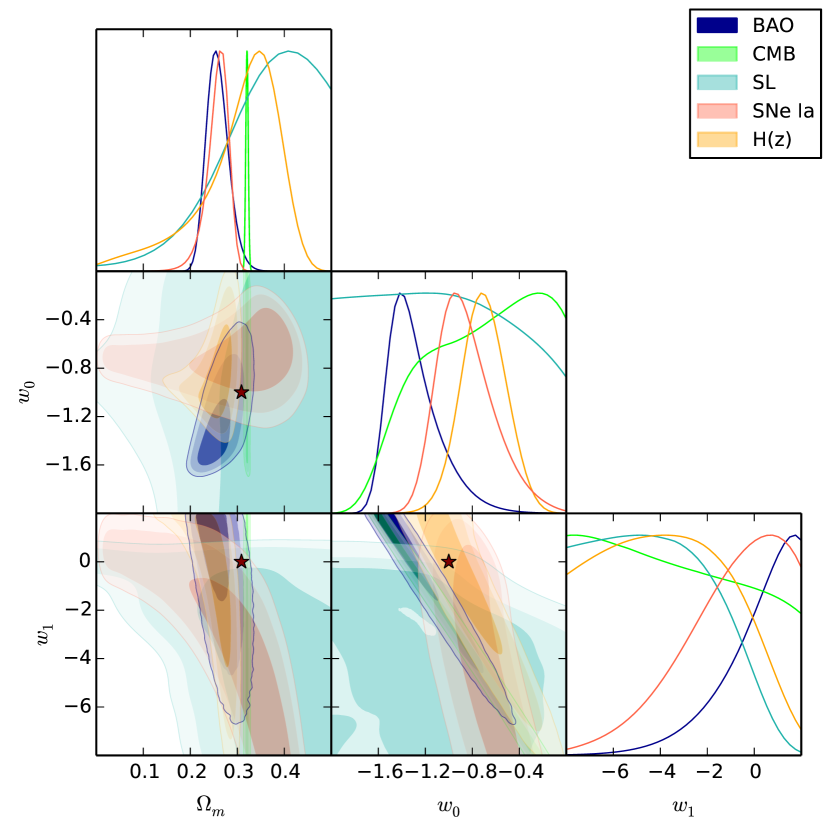
Figure 4: Confidence contours (1$\sigma$, 2$\sigma$, 3$\sigma$) and the marginalized 1-dimensional posterior probability distributions on the $\Omega_{m}$, $w_{0}$ and $w_{1}$ parameters for the cosmological model JBP for Abell 1689 with $\delta_{pos}=1.0\arcsec$. The star indicates the cosmological parameters as constrained by Planck Collaboration et al. (2016b) for a $\mathrm{\Lambda_{CDM}}$ cosmology.

The main indicator for the quality of the cosmological constraints is provided by the FOM values. Although there is not a clear tendency FOM vs. $\delta_{pos}$, the strong constraints for the BA, FSLL I, FSLL II and SeLa parameters are obtained when $\delta_{pos}=0.25\arcsec$. However, this uncertainty can lead to a poor cluster model. Moreover, this error provide SL confidence contours only consistent within the $3\sigma$ confidence levels with those obtained from the other cosmological tests. The optimum fit is obtained as a compromise between those $\chi_{red}$ and RMS values that provide a good lens model and the FOM value that gives cosmological constraints that are also in agreement with other probes. Thus, in the following, we discuss the parameter estimation for the case in which those criteria are fulfilled (i.e. $\delta_{pos}=1\arcsec$, see Figure 4 and Appendix B).

Figure 1: Comparison of the constraints on the $\mathrm{\Omega_{m}}$-$w_{0}$ parameters for Ares (left panel) and Abell1689 (right panel) when considering several positional uncertainties ($\delta_{pos}$) in the SL modeling for the JBP parameters. The star indicates the reference fiducial values. The mean values when $\delta_{pos}$ is $0.25\arcsec$, $0.5\arcsec$, and $1.0\arcsec$ are represented by the diamond, pentagon and triangle respectively.

4.2 $w(z)$ parameter estimations from SL in Abell 1689

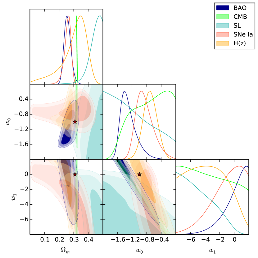
Figure 2: Confidence contours (1$\sigma$, 2$\sigma$, 3$\sigma$) and the marginalized 1-dimensional posterior probability distributions on the $\Omega_{m}$, $w_{0}$ and $w_{1}$ parameters for the cosmological model JBP for Abell 1689 with $\delta_{pos}=0.25\arcsec$. The star indicates the cosmological parameters as constrained by Planck Collaboration et al. (2016b) for a $\mathrm{\Lambda_{CDM}}$ cosmology.

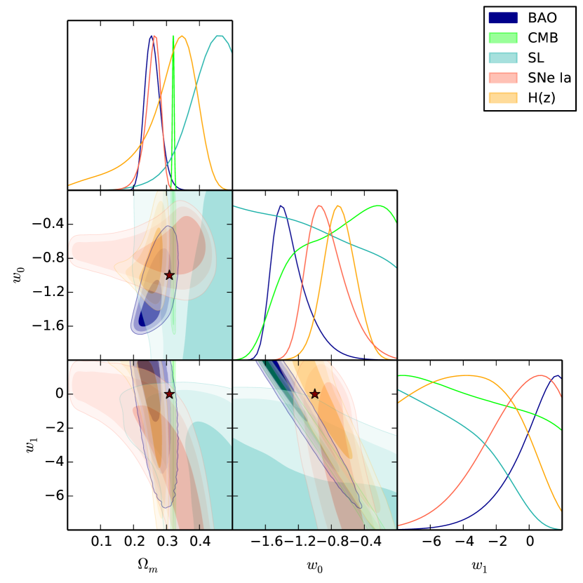
Figure 3: Confidence contours (1$\sigma$, 2$\sigma$, 3$\sigma$) and the marginalized 1-dimensional posterior probability distributions on the $\Omega_{m}$, $w_{0}$ and $w_{1}$ parameters for the cosmological model JBP for Abell 1689 with $\delta_{pos}=0.5\arcsec$. The star indicates the cosmological parameters as constrained by Planck Collaboration et al. (2016b) for a $\mathrm{\Lambda_{CDM}}$ cosmology.

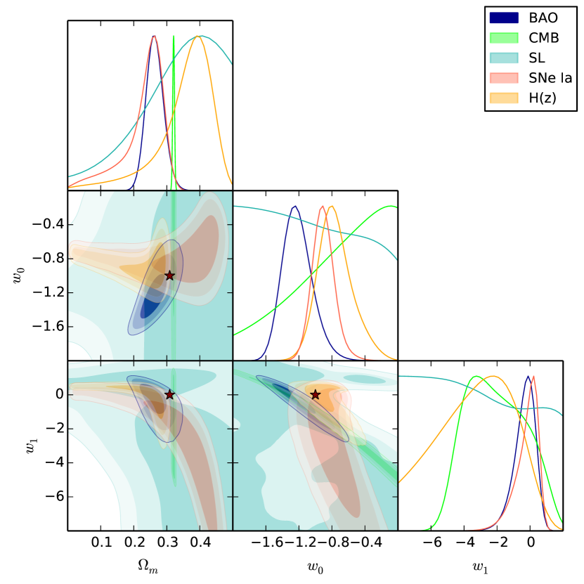
Figure B1: The same as Fig. 4 for the BA parameterization.

In general, for all models, we found that the SL technique using Abell 1689 data provides better $\Omega_{m}$ constraints than the ones on the equation of state parameters and confirm our previous result: a larger error ($\delta_{pos}=1\arcsec$) provides more significant constraints for the cluster parameters, i.e. $\chi_{red}\sim 1$, and reasonable RMS values. As in the Ares case, the right panel of the Figure 1 shows that increasing $\delta_{pos}$ is translated into an enlargement of the confidence contours and a systematic shift in the $\Omega_{m0}$ estimation towards the fiducial value. In addition, although this uncertainty produce the lowest FOM values (i.e. less significant cosmological parameters) for all $w(z)$ parametrizations, the confidence contours are in complete agreement with those of the other probes. The Figures 2-4 show the 1$\sigma$, 2$\sigma$, 3$\sigma$ confidence contours and the marginalized 1-dimensional posterior probability distributions on the $\Omega_{m}$, $w_{0}$, $w_{1}$ parameters for the cosmological model JBP using Abell 1689 SL data for each positional uncertainty considered. We note again that, when the error in the image position is increased, the $\Omega_{m}-w_{0}$ and $\Omega_{m}-w_{1}$ (or $w_{0}-w_{1}$) confidence contours shift towards the left (upper) region, where the confidence contours from BAO, CMB, SNe Ia, and H(z) probes are overlapped. This same trend is recovered for the BA, FSLL I, FSLL II and SeLa parameterizations (their confidence contours are provided in the Figs. B1-B4 of the Appendix B).

On the other hand, the $w_{0}$ and $w_{1}$ mean values for the five $w(z)$ parameterizations could suggest a dynamical equation of state, which can be associated to thawing or freezing quintessence DE (Pantazis et al., 2016). Nevertheless, all our EoS constraints are consistent with the cosmological constant, i.e. $w_{0}=-1$, and $w_{1}=0$, within the $3\sigma$ confidence level. In addition, there is no significant difference among the $\chi^{2}_{red}$ and RMS values for different $w(z)$ parameterizations. Therefore, any parametric DE model could be the source of the late cosmic acceleration. We confirm this result in the left panel of the Figure 5 which shows the reconstruction of the cosmological evolution for each parameterization using the mean values obtained from the SL modeling in Abell 1689 when $\delta_{pos}=1\arcsec$ is considered.

4.3 Deceleration parameter

The cosmological behavior of the deceleration parameter (Eq. 5) is an important test to know whether a DE model is able to handle the late cosmic acceleration. The right panels of Figure 5 shows the reconstructed $q(z)$ evolution for each parameterization obtained from Abell 1689 SL data when the multiple image-positional error is $1\arcsec$. We also have propagated its error within the $1\sigma$ confidence level using a Monte Carlo approach. Notice that the five cosmological models predict an accelerating expansion at late times. The transition redshifts, i.e. when the Universe passes from an decelerated phase to one accelerated, are $z_{t}={0.44^{+0.21}_{-0.17},0.44^{+0.17}_{-0.12},0.45^{+0.18}_{-0.13},0.50^{+0.22}_{-0.24},0.34^{+0.07}_{-0.04}}$ for the JBP, BA, FSLL I, FSLL II, and SeLa parameterizations, respectively. Furthermore, the $q(z)$ shape for each parameterization is consistent with that of the cosmological constant within the $1\sigma$ confidence level.

Table 1: JBP mean fit parameters obtained for both galaxy clusters SL data. The columns give the reduced $\chi^{2}_{red}$, RMS in the image plane (in arcseconds) and the mean values for $\Omega_{m}$, $w_{0}$, $w_{1}$ with $68\%$ confidence level errors. The mean values estimated with H(z), SNIa, BAO and CMB data are also provided.

Cluster name	Error in the pos. ($\arcsec$)	$\chi^{2}_{red}$	RMS ($\arcsec$)	FOM	$\Omega_{m}$	$w_{0}$	$w_{1}$
Abell 1689	0.25	11.37	0.54	15.09	$0.47_{-0.06}^{+0.04}$	$-1.29_{-0.01}^{+1.04}$	$-6.46_{-0.33}^{+4.88}$
Ares		2.73	0.59	127.92	$0.37_{-0.11}^{+0.12}$	$-0.82_{-0.11}^{+0.11}$	$-0.14_{-0.04}^{+0.36}$
Abell 1689	0.5	3.14	0.64	8.13	$0.46_{-0.08}^{+0.08}$	$-1.11_{-0.04}^{+1.20}$	$-6.14_{-0.07}^{+5.49}$
Ares		0.78	0.65	11.83	$0.46_{-0.11}^{+0.06}$	$-0.90_{-0.49}^{+0.60}$	$-1.77_{-3.01}^{+0.07}$
Abell 1689	1.0	0.95	0.88	4.15	$0.43_{-0.12}^{+0.18}$	$-1.07_{-0.60}^{+0.69}$	$-5.09_{-3.40}^{+3.07}$
Ares		0.77	0.94	20.46	$0.33_{-0.06}^{+0.06}$	$-1.06_{-0.43}^{+0.83}$	$-5.81_{-3.16}^{+3.41}$
Complementary probes
H(z)	—	$0.54$	—	354.12	$0.26^{+0.01}_{-0.02}$	$-0.88^{+0.27}_{-0.19}$	$-0.70^{+1.83}_{-2.59}$
SNIa	—	$0.98$	—	75.51	$0.32^{+0.05}_{-0.10}$	$-0.70^{+0.19}_{-0.18}$	$-4.44^{+3.40}_{-3.49}$
BAO	—	$2.17$	—	646.43	$0.25^{+0.02}_{-0.02}$	$-1.34^{+0.26}_{-0.15}$	$0.43^{+1.13}_{-1.99}$
CMB	—	$58.8$	—	8207.46	$0.32^{+0.002}_{-0.002}$	$-0.69^{+0.50}_{-0.68}$	$-4.54^{+4.26}_{-3.66}$

Table 2: The same as Table 4.3 for the BA parameterization.

Cluster name	Error in the pos. ($\arcsec$)	$\chi^{2}_{red}$	RMS ($\arcsec$)	FOM	$\Omega_{m}$	$w_{0}$	$w_{1}$
Abell 1689	0.25”	11.40	0.54	13.57	$0.47_{-0.06}^{+0.05}$	$-1.32_{-0.01}^{+0.98}$	$-6.28_{-0.07}^{+5.31}$
Ares		2.69	0.59	5.25	$0.27_{-0.01}^{+0.46}$	$-0.89_{-0.48}^{+0.16}$	$0.09_{-1.10}^{+0.91}$
Abell 1689	0.5”	3.15	0.64	6.22	$0.44_{-0.10}^{+0.08}$	$-1.15_{-0.02}^{+1.20}$	$-5.22_{-0.57}^{+6.17}$
Ares		0.80	0.65	8.25	$0.20_{-0.01}^{+0.36}$	$-1.10_{-0.24}^{+0.31}$	$0.36_{-1.81}^{+0.16}$
Abell 1689	1.0”	0.94	0.89	3.26	$0.41_{-0.15}^{+0.17}$	$-1.08_{-0.02}^{+1.26}$	$-4.49_{-7.69}^{+0.62}$
Ares		0.33	0.93	6.91	$0.26_{-0.0}^{+0.31}$	$-1.37_{-0.24}^{+0.31}$	$-1.88_{-6.28}^{+0.18}$
Complementary probes
H(z)	—	$0.57$	—	405.21	$0.25^{+0.02}_{-0.08}$	$-0.90^{+0.13}_{-0.12}$	$0.01^{+0.43}_{-0.85}$
SNIa	—	$0.98$	—	70.47	$0.37^{+0.04}_{-0.09}$	$-0.78^{+0.22}_{-0.17}$	$-3.24^{+2.37}_{-3.14}$
BAO	—	$2.25$	—	1541.69	$0.26^{+0.02}_{-0.02}$	$-1.23^{+0.18}_{-0.16}$	$-0.23^{+0.52}_{-0.69}$
CMB	—	$58.8$	—	3492.21	$0.32^{+0.002}_{-0.002}$	$-0.63^{+0.45}_{-0.67}$	$-2.24^{+2.18}_{-1.82}$

Table 3: The same as Table 4.3 for the FSLL I parameterization.

Cluster name	Error in the pos. ($\arcsec$)	$\chi^{2}_{red}$	RMS ($\arcsec$)	FOM	$\Omega_{m}$	$w_{0}$	$w_{1}$
Abell 1689	0.25”	11.53	0.54	12.67	$0.46_{-0.06}^{+0.05}$	$-1.39_{-0.04}^{+0.93}$	$-6.60_{-0.07}^{+5.04}$
Ares		2.70	0.59	168.03	$0.17_{-0.03}^{+0.22}$	$-0.99_{-0.16}^{+0.24}$	$0.48_{-0.72}^{+0.29}$
Abell 1689	0.5”	3.07	0.64	4.10	$0.42_{-0.12}^{+0.09}$	$-1.17_{-0.21}^{+1.08}$	$-4.75_{-8.73}^{+0.14}$
Ares		0.80	0.65	11.29	$0.23_{-0.02}^{+0.36}$	$-1.36_{-0.15}^{+0.60}$	$0.79_{-3.00}^{+0.08}$
Abell 1689	1.0”	0.93	0.89	3.34	$0.40_{-0.15}^{+0.17}$	$-1.15_{-0.16}^{+1.07}$	$-4.99_{-1.12}^{+6.08}$
Ares		0.33	0.92	8.03	$0.27_{-0.01}^{+0.32}$	$-1.45_{-0.15}^{+0.97}$	$-1.89_{-7.13}^{+0.13}$
Complementary probes
H(z)	—	$0.48$	—	268.56	$0.25^{+0.02}_{-0.06}$	$-0.95^{+0.19}_{-0.15}$	$0.14^{+1.03}_{-1.46}$
SNIa	—	$0.98$	—	71.57	$0.36^{+0.05}_{-0.10}$	$-0.74^{+0.22}_{-0.18}$	$-3.77^{+2.77}_{-3.37}$
BAO	—	$2.13$	—	1014.38	$0.24^{+0.02}_{-0.02}$	$-1.40^{+0.25}_{-0.19}$	$0.51^{+0.92}_{-1.24}$
CMB	—	$58.8$	—	5455.18	$0.32^{+0.002}_{-0.002}$	$-0.69^{+0.50}_{-0.68}$	$-2.86^{+3.05}_{-2.54}$

Table 4: The same as Table 4.3 for the FSLL II parameterization.

Cluster name	Error in the pos. ($\arcsec$)	$\chi^{2}_{red}$	RMS ($\arcsec$)	FOM	$\Omega_{m}$	$w_{0}$	$w_{1}$
Abell 1689	0.25”	11.90	0.54	19.78	$0.41_{-0.06}^{+0.05}$	$-1.61_{-0.03}^{+0.54}$	$-5.59_{-0.09}^{+6.82}$
Ares		2.71	0.59	50.04	$0.19_{-0.01}^{+0.33}$	$-0.81_{-0.10}^{+0.06}$	$0.18_{-0.80}^{+0.13}$
Abell 1689	0.5”	3.17	0.64	7.96	$0.38_{-0.10}^{+0.09}$	$-1.45_{-0.26}^{+0.57}$	$-4.81_{-0.29}^{+7.24}$
Ares		0.79	0.65	8.74	$0.38_{-0.21}^{+0.15}$	$-1.00_{-0.44}^{+0.25}$	$-0.64_{-4.69}^{+0.38}$
Abell 1689	1.0”	0.94	0.89	3.31	$0.35_{-0.14}^{+0.20}$	$-1.29_{-0.31}^{+0.70}$	$-4.78_{-0.10}^{+7.57}$
Ares		0.32	0.92	9.50	$0.28_{-0.14}^{+0.06}$	$-1.35_{-0.54}^{+0.29}$	$-2.11_{-7.14}^{+0.50}$
Complementary probes
H(z)	—	$0.56$	—	164.36	$0.26^{+0.02}_{-0.06}$	$-0.92^{+0.11}_{-0.10}$	$-0.30^{+0.92}_{-2.12}$
SNIa	—	$0.98$	—	71.30	$0.32^{+0.04}_{-0.11}$	$-0.98^{+0.15}_{-0.15}$	$-4.34^{+3.90}_{-3.86}$
BAO	—	$2.21$	—	530.10	$0.27^{+0.02}_{-0.02}$	$-1.19^{+0.12}_{-0.10}$	$-1.34^{+1.23}_{-1.91}$
CMB	—	$58.8$	—	2702.46	$0.32^{+0.002}_{-0.002}$	$-0.87^{+0.22}_{-0.34}$	$-4.96^{+4.01}_{-3.51}$

Table 6: The same as Table 4.3 for the SeLa parameterization.

Cluster name	Error in the pos. ($\arcsec$)	$\chi^{2}_{red}$	RMS ($\arcsec$)	FOM	$\Omega_{m}$	$w_{0}$	$w_{0.5}$
Abell 1689	0.25”	11.66	0.54	43.94	$0.42_{-0.10}^{+0.07}$	$-1.23_{-0.24}^{+0.94}$	$0.61_{-1.57}^{+0.38}$
Ares		6.01	4.80	33.84	$0.80_{-0.09}^{+0.06}$	$-1.04_{-0.08}^{+1.25}$	$0.38_{-1.56}^{+0.65}$
Abell 1689	0.5”	3.06	0.64	25.21	$0.41_{-0.09}^{+0.11}$	$-1.18_{-0.13}^{+1.06}$	$-0.54_{-1.96}^{+0.02}$
Ares		1.57	1.11	25.09	$0.66_{-0.09}^{+0.12}$	$-1.26_{-0.01}^{+1.07}$	$-0.59_{-1.83}^{+0.14}$
Abell 1689	1.0”	0.93	0.90	12.67	$0.46_{-0.05}^{+0.04}$	$-1.39_{-0.44}^{+0.73}$	$-6.60_{-2.44}^{+3.87}$
Ares		0.48	1.06	23.61	$0.41_{-0.10}^{+0.16}$	$-1.16_{-0.04}^{+1.17}$	$0.49_{-1.40}^{+0.79}$
Complementary probes
H(z)	—	$0.55$	—	703.29	$0.25^{+0.02}_{-0.07}$	$-0.90^{+0.14}_{-0.12}$	$-1.01^{+0.31}_{-0.36}$
SNIa	—	$0.98$	—	111.75	$0.37^{+0.05}_{-0.09}$	$-0.73^{+0.28}_{-0.18}$	$-2.64^{+1.23}_{-1.57}$
BAO	—	$9.95$	—	377.94	$0.23^{+0.04}_{-0.08}$	$-1.04^{+0.28}_{-0.23}$	$-1.11^{+0.55}_{-0.37}$
CMB	—	$58.8$	—	1004.52	$0.32^{+0.002}_{-0.002}$	$-0.56^{+0.40}_{-0.54}$	$-1.98^{+0.51}_{-0.50}$

5 conclusions

Several recent studies have shown that dark energy could deviate from a cosmological constant (Ferreira et al., 2017; Zhao et al., 2017). A simple way to investigate such alternative dark energy models is to parameterize the dark energy equation of state as a function of redshift. In order to elucidate the nature of dark energy, numerous parameterizations have been proposed (see for instance Pantazis et al., 2016, and references therein). The typical tests to constrain cosmological parameters use SNe Ia, H(z), BAO and CMB distance posterior measurements. Nevertheless, some of them could provide biased constraints because either the data or the test fitting formulae are derived assuming an underlying standard cosmology (see Appendix A). Furthermore, new complementary techniques could break the degeneracy between parameters and obtain stringent constraints which could help us distinguish the nature of dark energy.

In this paper, which is the first in a series, we investigate a promising technique to study alternative cosmological models and to constrain their parameters using the strong lensing features in galaxy clusters. This method has the advantage of providing constraints which are not biased due to an underlying cosmology.

We have considered the following five popular bi-parametric CPL-like ansatz: JBP, BA, FSLL I, FSLL II, and SeLa and constrained their parameters using the SL data in a real galaxy cluster, Abell 1689, and a simulated one Ares. We implemented these $w(z)$ parameterizations in the LENSTOOL code which uses a MCMC algorithm to simultaneously constrain the lens model and the $w(z)$ parameters. In addition, we have considered three different image-positional errors to quantify how the cosmological constraints are affected by these uncertainties in the lens modeling. In general, we found that the SL technique provides competitive constraints on the $w(z)$ parameters in comparison with the common cosmological tests. Moreover, when increasing the image-positional error (from $0.5\arcsec$ to $1.0\arcsec$), we find that systematic biases with respect to the known input cosmological values in the simulated cluster decrease. After taking this calibration into account in the real data, our SL constraints are consistent with those obtained from other probes.

In summary, we have exploited the strong lensing modeling in galaxy clusters as a cosmological probe. Although we have measured competitive constraints on the $w(z)$ parameters, further analysis on the galaxy clusters and their environment is needed to improve the strong lensing modeling and hence to more tightly estimate cosmological parameters. In forthcoming papers, we will test this method to constrain the parameter of other cosmological scenarios, for instance, those considering interactions in the dark sector.

Figure 5: Reconstructed equation of state (left panel) and deceleration parameter (right panel) vs. redshift for each $w(z)$ parameterization using the mean values obtained from SL data in Abell 1689 with an image-position error of $1.0\arcsec$. The shadow regions show the $1\sigma$ region calculated with a MCMC error propagation approach using the SL posterior constraints.

Appendix A Additional cosmological data

We compare the constraints obtained from the strong lensing modeling with those from BAO, CMB, SNe Ia and H(z) cosmological probes. In the following we describe briefly these cosmological data, for further details on how their figure-of-merit is constructed see Magaña et al. (2015, 2017) and references therein.

A.1 BAO

Large-scale galaxy surveys offer the possibility of measuring the signature of Baryon Acoustic Oscillations which is a typical length scale imprinted in both photons and baryons by the propagation of sound waves in the primordial plasma of the Universe. This signal, i.e. the sound horizon at the drag epoch, $r_{s}(z_{d})$, is a standard ruler which can be used to test alternative cosmologies. To complement our SL constraints, we use the following 9 BAO points (see Magaña et al., 2017, and references therein)to constrain the $w(z)$ functions:

• 6dFGS.- $z=0.106,dz\equiv\frac{r_{s}(z_{d})}{D_{V}(z)}=0.336\pm 0.015$, where $D_{V}(z)=\frac{1}{H_{0}}\left[(1+z)^{2}D(z)^{2}\frac{cz}{E(z)}\right]^{1/3}$

• WiggleZ.- $z=\left[0.44,0.6,0.73\right]$, $dz=\left[0.0870\pm 0.0042,0.0672\pm 0.0031,0.0593\pm 0.0020\right]$

• SDSS DR7 $z=0.15,0.2239\pm 0.0084$

• SDSS-III BOSS DR11 (a).- $z=\left[0.32,57\right]$, $dz=\left[0.1181\pm 0.0022,0.0726\pm 0.0007\right]$

• SDSS-III BOSS DR11 (b).- $z=\left[2.34,2.36\right]$, $\frac{D_{H}(z)}{r_{s}(z_{d})}=\left[9.18\pm 0.28,9.00\pm 0.3\right]$, where $D_{H(z)}=c/H_{0}E(z)$

It is worth noting that $r_{s}(z_{d})$ depends on the underlying cosmology which is commonly the $\Lambda$CDM model. Moreover, the $z_{d}$ formulae employed in the BAO fitting (Eisenstein & Hu, 1998) were calculated for the standard cosmology. Thus, the BAO constraints could be biased due to the standard cosmology.

A.2 Distance posteriors from CMB Planck 2015 measurements

The information of the CMB acoustic peaks can be compressed in three quantities, their distance posteriors: the acoustic scale, $l_{A}$, the shift parameter, $R$, and the decoupling redshift, $z_{*}$. Several authors have proved that these quantities are almost independent of the input DE models (Wang et al., 2012). Thus, to constrain the $w(z)$ parameters we use the following distance posteriors for a flat $w$CDM, estimated by Neveu et al. (2017) from Planck 2015 measurements: $l_{A}^{obs}=301.787\pm 0.089$, $R^{obs}=1.7492\pm 0.0049$, $z_{*}^{obs}=1089.99\pm 0.29$.

It is worth noting that the fitting formulae for these quantities (Hu & Sugiyama, 1996; Bond et al., 1997) are calculated for the standard model, however we assume that they are valid in dynamical DE models.

A.3 SNe Ia

Since that Type Ia Supernovae are standard candles, i.e. their light curves have the same shape after a standardization process, they have been used to measure cosmological parameters. Indeed, the apparent cosmic accelerating expansion was observed through a Hubble diagram of distant SNIa. As complementary test, we consider the compilation by Ganeshalingam et al. (2013) which contains 586 data points of the modulus distance, $\mu$, in the redshift range $0.01<z<1.4$ which include mainly 91 points from the Lick Observatory Supernova Search (LOSS) SN Ia observations.

A.4 H(z) measurements

The Hubble parameter at different redshifts provide a direct measurement of the expansion rate of the Universe. Several authors have estimated the observational Hubble data using different techniques: from clustering or BAO peaks (see for instance, Gaztanaga et al., 2009) and from cosmic chronometers (Jimenez & Loeb, 2002). Here, we use the same sample used by Magaña et al. (2017) which contains $34$ data points in the redshift range $0.07<z<2.36$. Although some of the H(z) points were estimated from BAO data, we assume that there is no correlation between them. It is worth noting that the $H(z)$ points obtained from BAO could yield to biased constraints due to the underlying ($\Lambda$CDM) cosmology on $r_{s}(z_{d}).$

Appendix B Confidence Contours for the BA, FSLL I, FSLL II and SeLa parameterizations

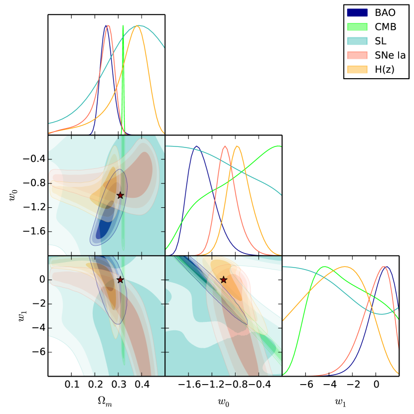
Figure B2: The same as Fig. 4 for the FSLL I parameterization.

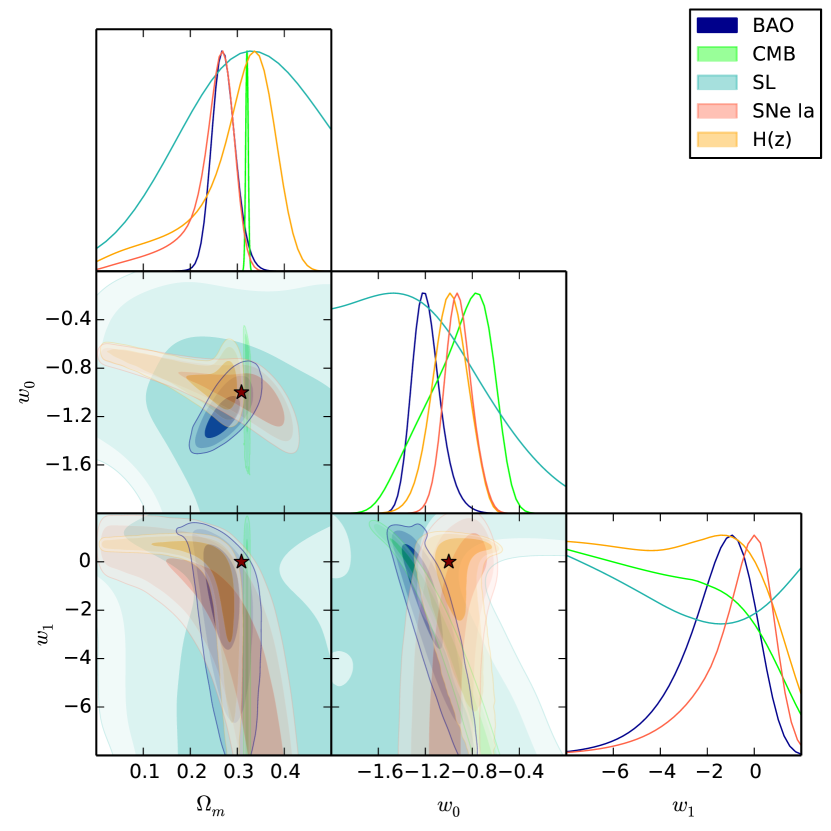
Figure B3: The same as Fig. 4 for the FSLL II parameterization.

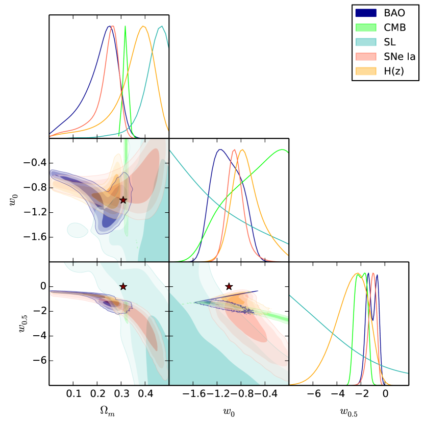
Figure B4: The same as Fig. 4 for the SeLa parameterization.

References

- Acebron et al. (2017) Acebron, A., Jullo, E., Limousin, M., et al. 2017, ArXiv e-prints, arXiv:1704.05380
- Albrecht et al. (2006) Albrecht, A., Bernstein, G., Cahn, R., et al. 2006, ArXiv Astrophysics e-prints, astro-ph/0609591
- Barboza & Alcaniz (2008) Barboza, E. M., & Alcaniz, J. S. 2008, Physics Letters B, 666, 415
- Bayliss et al. (2014) Bayliss, M. B., Johnson, T., Gladders, M. D., Sharon, K., & Oguri, M. 2014, ApJ, 783, 41
- Bina et al. (2016) Bina, D., Pelló, R., Richard, J., et al. 2016, A&A, 590, A14
- Bond et al. (1997) Bond, J. R., Efstathiou, G., & Tegmark, M. 1997, MNRAS, 291, L33
- Caminha et al. (2016) Caminha, G. B., Grillo, C., Rosati, P., et al. 2016, A&A, 587, A80
- Chevallier & Polarski (2001) Chevallier, M., & Polarski, D. 2001, International Journal of Modern Physics D, 10, 213
- Chirivì et al. (2018) Chirivì, G., Suyu, S. H., Grillo, C., et al. 2018, A&A, 614, A8
- Copeland et al. (2006) Copeland, E. J., Sami, M., & Tsujikawa, S. 2006, International Journal of Modern Physics D, 15, 1753
- D’Aloisio & Natarajan (2011) D’Aloisio, A., & Natarajan, P. 2011, MNRAS, 411, 1628
- Davis (2014) Davis, T. M. 2014, General Relativity and Gravitation, 46, 1731
- Diego et al. (2015) Diego, J. M., Broadhurst, T., Benitez, N., et al. 2015, MNRAS, 446, 683
- Eisenstein & Hu (1998) Eisenstein, D. J., & Hu, W. 1998, ApJ, 496, 605
- Elíasdóttir et al. (2007) Elíasdóttir, Á., Limousin, M., Richard, J., et al. 2007, ArXiv e-prints, arXiv:0710.5636
- Feng et al. (2012) Feng, C.-J., Shen, X.-Y., Li, P., & Li, X.-Z. 2012, J. Cosmology Astropart. Phys, 9, 023
- Ferreira et al. (2017) Ferreira, E. G. M., Quintin, J., Costa, A. A., Abdalla, E., & Wang, B. 2017, Phys. Rev. D, 95, 043520
- Foreman-Mackey et al. (2013) Foreman-Mackey, D., Hogg, D. W., Lang, D., & Goodman, J. 2013, PASP, 125, 306
- Ganeshalingam et al. (2013) Ganeshalingam, M., Li, W., & Filippenko, A. V. 2013, MNRAS, 433, 2240
- Gaztanaga et al. (2009) Gaztanaga, E., Cabre, A., & Hui, L. 2009, Mon. Not. Roy. Astron. Soc., 399, 1663
- Giocoli et al. (2016) Giocoli, C., Bonamigo, M., Limousin, M., et al. 2016, MNRAS, 462, 167
- Giocoli et al. (2012) Giocoli, C., Meneghetti, M., Bartelmann, M., Moscardini, L., & Boldrin, M. 2012, MNRAS, 421, 3343
- Golse et al. (2002) Golse, G., Kneib, J.-P., & Soucail, G. 2002, A&A, 387, 788
- Grillo et al. (2015) Grillo, C., Suyu, S. H., Rosati, P., et al. 2015, ApJ, 800, 38
- Harvey et al. (2016) Harvey, D., Kneib, J. P., & Jauzac, M. 2016, MNRAS, 458, 660
- Host (2012) Host, O. 2012, MNRAS, 420, L18
- Hu & Sugiyama (1996) Hu, W., & Sugiyama, N. 1996, ApJ, 471, 542
- Jaroszynski & Kostrzewa-Rutkowska (2014) Jaroszynski, M., & Kostrzewa-Rutkowska, Z. 2014, MNRAS, 439, 2432
- Jassal et al. (2005a) Jassal, H. K., Bagla, J. S., & Padmanabhan, T. 2005a, Phys. Rev. D, 72, 103503
- Jassal et al. (2005b) —. 2005b, MNRAS, 356, L11
- Jauzac et al. (2014) Jauzac, M., Clément, B., Limousin, M., et al. 2014, MNRAS, 443, 1549
- Jimenez & Loeb (2002) Jimenez, R., & Loeb, A. 2002, Astrophys. J., 573, 37
- Joyce et al. (2016) Joyce, A., Lombriser, L., & Schmidt, F. 2016, Annual Review of Nuclear and Particle Science, 66, 95
- Jullo et al. (2007) Jullo, E., Kneib, J.-P., Limousin, M., et al. 2007, MNRAS, 9, 447
- Jullo et al. (2010) Jullo, E., Natarajan, P., Kneib, J.-P., et al. 2010, Science, 329, 924
- Kassiola & Kovner (1993) Kassiola, A., & Kovner, I. 1993, ApJ, 417, 450
- Kneib et al. (1996) Kneib, J.-P., Ellis, R. S., Smail, I., Couch, W. J., & Sharples, R. M. 1996, ApJ, 471, 643
- Komatsu et al. (2011) Komatsu, E., et al. 2011, Astrophys. J. Suppl., 192, 18
- Lazkoz et al. (2005) Lazkoz, R., Nesseris, S., & Perivolaropoulos, L. 2005, J. Cosmology Astropart. Phys, 11, 010
- Li et al. (2011) Li, M., Li, X.-D., Wang, S., & Wang, Y. 2011, Communications in Theoretical Physics, 56, 525
- Limousin et al. (2005) Limousin, M., Kneib, J.-P., & Natarajan, P. 2005, MNRAS, 356, 309
- Limousin et al. (2013) Limousin, M., Morandi, A., Sereno, M., et al. 2013, Space Sci. Rev., 177, 155
- Limousin et al. (2007) Limousin, M., Richard, J., Jullo, E., et al. 2007, ApJ, 668, 643
- Limousin et al. (2010) Limousin, M., Jullo, E., Richard, J., et al. 2010, A&A, 524, A95
- Limousin et al. (2016) Limousin, M., Richard, J., Jullo, E., et al. 2016, A&A, 588, A99
- Linder (2003) Linder, E. V. 2003, Physical Review Letters, 90, 091301
- Link & Pierce (1998) Link, R., & Pierce, M. J. 1998, ApJ, 502, 63
- Magaña et al. (2014) Magaña, J., Cárdenas, V. H., & Motta, V. 2014, JCAP, 1410, 017
- Magaña et al. (2017) Magaña, J., Motta, V., Cárdenas, V. H., & Foëx, G. 2017, MNRAS, 469, 47
- Magaña et al. (2015) Magaña, J., Motta, V., Cardenas, V. H., Verdugo, T., & Jullo, E. 2015, Astrophys. J., 813, 69
- McCully et al. (2014) McCully, C., Keeton, C. R., Wong, K. C., & Zabludoff, A. I. 2014, MNRAS, 443, 3631
- McCully et al. (2017) —. 2017, ApJ, 836, 141
- Meneghetti et al. (2016) Meneghetti, M., Natarajan, P., Coe, D., et al. 2016, ArXiv e-prints, arXiv:1606.04548
- Miralda-Escude & Babul (1995) Miralda-Escude, J., & Babul, A. 1995, ApJ, 449, 18
- Monna et al. (2017) Monna, A., Seitz, S., Balestra, I., et al. 2017, MNRAS, arXiv:1605.08784
- Mortonson et al. (2014) Mortonson, M. J., Weinberg, D. H., & White, M. 2014, ArXiv e-prints, arXiv:1401.0046
- Neveu et al. (2017) Neveu, J., Ruhlmann-Kleider, V., Astier, P., et al. 2017, A&A, 600, A40
- Pantazis et al. (2016) Pantazis, G., Nesseris, S., & Perivolaropoulos, L. 2016, Phys. Rev. D, 93, 103503
- Perlmutter et al. (1999) Perlmutter, S., Aldering, G., Goldhaber, G., et al. 1999, The Astrophysical Journal, 517, 565
- Planck Collaboration et al. (2016a) Planck Collaboration, Ade, P. A. R., Aghanim, N., et al. 2016a, A&A, 594, A13
- Planck Collaboration et al. (2016b) —. 2016b, A&A, 594, A14
- Riess et al. (1998) Riess, A. G., Filippenko, A. V., Challis, P., et al. 1998, The Astronomical Journal, 116, 1009
- Salvatelli et al. (2014) Salvatelli, V., Said, N., Bruni, M., Melchiorri, A., & Wands, D. 2014, Phys. Rev. Lett., 113, 181301
- Sendra & Lazkoz (2012) Sendra, I., & Lazkoz, R. 2012, MNRAS, 422, 776
- Soucail et al. (2004) Soucail, G., Kneib, J.-P., & Golse, G. 2004, A&A, 417, L33
- Tu et al. (2008) Tu, H., Limousin, M., Fort, B., et al. 2008, MNRAS, 386, 1169
- Umetsu et al. (2015) Umetsu, K., Sereno, M., Medezinski, E., et al. 2015, ApJ, 806, 207
- Wang et al. (2006) Wang, L., Li, C., Kauffmann, G., & De Lucia, G. 2006, MNRAS, 371, 537
- Wang et al. (2016) Wang, S., Hu, Y., Li, M., & Li, N. 2016, ApJ, 821, 60
- Wang (2008) Wang, Y. 2008, Phys. Rev. D, 77, 123525
- Wang et al. (2012) Wang, Y., Chuang, C.-H., & Mukherjee, P. 2012, Phys. Rev. D, 85, 023517
- Weinberg (1989) Weinberg, S. 1989, Reviews of Modern Physics, 61
- Zeldovich (1968) Zeldovich, Y. B. 1968, Soviet Physics Uspekhi, 11
- Zhao et al. (2017) Zhao, G.-B., Raveri, M., Pogosian, L., et al. 2017, Nature Astronomy, 1, 627
- Zitrin et al. (2012) Zitrin, A., Rosati, P., Nonino, M., et al. 2012, The Astrophysical Journal, 749, 97
- Zitrin et al. (2015) Zitrin, A., Fabris, A., Merten, J., et al. 2015, ApJ, 801, 44