Medoids in almost linear time via multi-armed bandits

Abstract

Computing the medoid of a large number of points in high-dimensional space is an increasingly common operation in many data science problems. We present an algorithm Med-dit which uses $O(n\log n)$ distance evaluations to compute the medoid with high probability. Med-dit is based on a connection with the multi-armed bandit problem. We evaluate the performance of Med-dit empirically on the Netflix-prize and the single-cell RNA-Seq datasets, containing hundreds of thousands of points living in tens of thousands of dimensions, and observe a $5$-$10$x improvement in performance over the current state of the art. Med-dit is available at https://github.com/bagavi/Meddit.

1 INTRODUCTION

An important building block in many modern data analysis problems such as clustering is the efficient computation of a representative point for a large set of points in high dimension. A commonly used representative point is the centroid of the set, the point which has the smallest average distance from all other points in the set. For example, k-means clustering [28, 23, 21] computes the centroid of each cluster under the squared Euclidean distance. In this case, the centroid is the arithmetic mean of the points in the cluster, which can be computed very efficiently. Efficient computation of centroid is central to the success of k-means, as this computation has to be repeated many times in the clustering process.

While commonly used, centroid suffers from several drawbacks. First, the centroid is in general not a point in the dataset and thus may not be interpretable in many applications. This is especially true when the data is structured like in images, or when it is sparse like in recommendation systems [19]. Second, the centroid is sensitive to outliers: several far away points will significantly affect the location of the centroid. Third, while the centroid can be efficiently computed under squared Euclidean distance, there are many applications where using this distance measure is not suitable. Some examples would be applications where the data is categorical like medical records [29]; or situations where the data points have different support sizes such as in recommendation systems [19]; or cases where the data points are on a high-dimensional probability simplex like in single cell RNA-Seq analysis [25]; or cases where the data lives in a space with no well known Euclidean space like while clustering on graphs from social networks.

An alternative to the centroid is the medoid; this is the point in the set that minimizes the average distance to all the other points. It is used for example in $k$-medoids clustering [15]. On the real line, the medoid is the median of the set of points. The medoid overcomes the first two drawbacks of the centroid: the medoid is by definition one of the points in the dataset, and it is less sensitive to outliers than the centroid. In addition, centroid algorithms are usually specific to the distance used to define the centroid. On the other hand, medoid algorithms usually work for arbitrary distances.

The naive method to compute the medoid would require computing all pairwise distances between points in the set. For a set with $n$ points, this would require the computation of $\binom{n}{2}$ distances, which would be computationally prohibitive when there are hundreds of thousands of points and each point lives in a space with dimensions in tens of thousands.

In the one-dimensional case, the medoid problem reduces to the problem of finding the median, which can be solved in linear time through Quick-select [12]. However, in higher dimensions, no linear-time algorithm is known. RAND [8] is an algorithm that estimates the average distance of each point to all the other points by sampling a random subset of other points. It takes a total of $O\left(\frac{n\log n}{\epsilon}\right)$ distance computations to approximate the medoid within a factor of $(1+\epsilon\Delta)$ with high probability, where $\Delta$ is the maximum distance between two points in the dataset. We remark that this is an approximation algorithm, and moreover $\Delta$ may not be known apriori. RAND was leveraged by TOPRANK [26] which uses the estimates obtained by RAND to focus on a small subset of candidate points, evaluates the average distance of these points exactly, and picks the minimum of those. TOPRANK needs $O(n^{\frac{5}{3}}\log^{\frac{4}{3}}n)$ distance computations to find the exact medoid with high probability under a distributional assumption on the average distances. trimed [24] presents a clever algorithm to find the medoid with $O(n^{\frac{3}{2}}2^{\Theta(d)})$ distance evaluations, which works very well when the points live in a space of dimensions less than $20$ (i.e., $2^{d}\ll\sqrt{n}$) under a distributional assumption on the points (in particular on the distribution of points around the medoid). However, the exponential dependence on dimension makes it impractical when $d\geq 50$, which is the case we consider here. Note that their result requires the distance measure to satisfy the triangle inequality.

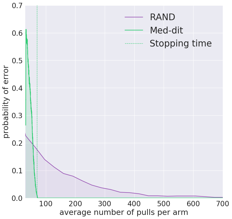
Figure 1: We plot the probability that RAND and Med-dit do not return the true medoid as a function of the number of distance evaluations per point over $1000$ monte-carlo trials. We note that Med-dit needs much fewer distance evaluations than RAND for comparable performance. The computation of the true medoid here is also computationally prohibitive and is discussed in Section 4.

In this paper, we present Med(oid)-(Ban)dit, a sampling-based algorithm that finds the exact medoid with high probability. It takes $O(n\log n)$ distance evaluations under natural assumptions on the distances, which are justified by the characteristics observed in real data (Section 2). In contrast to trimed, the number of distance computations is independent of the dimension $d$; moreover, there is no specific requirement for the distance measure, e.g. the triangle inequality or the symmetry. Thus, Med-dit is particularly suitable for high-dimensional data and general distance measures.

In Figure 1, we showcase the performance of RAND and Med-dit on the largest cluster of the single cell RNA-Seq gene expression dataset of [1]. This consists of $27,998$ gene-expressions of each of $109,140$ cells, $i.e$ $109,140$ points in $27,998$ dimensions. We note that Med-dit evaluates around $10$ times fewer distances than RAND to achieve similar performance. At this scale running TOPRANK and trimed are computationally prohibitive.

The main idea behind Med-dit is noting that the problem of computing the medoid can be posed as that of computing the best arm in a multi-armed bandit (MAB) setting [9, 13, 17]. One views each point in the medoid problem as an arm whose unknown parameter is its average distance to all the other points. Pulling an arm corresponds to evaluating the distance of that point to a randomly chosen point, which provides an estimate of the arm’s unknown parameter. We leverage the extensive literature on the multi-armed bandit problem to propose Med-dit, which is a variant of the Upper Confidence Bound (UCB) Algorithm [17].

Like the other sampling based algorithms RAND and TOPRANK, Med-dit also aims to estimate the average distance of every point to the other points by evaluating its distance to a random subset of points. However, unlike these algorithms where each point receives a fixed amount of sampling decided apriori, the sampling in Med-dit is done adaptively. More specifically, Med-dit maintains confidence intervals for the average distances of all points and adaptively evaluates distances of only those points which could potentially be the medoid. Loosely speaking, points whose lower confidence bound on the average distance are small form the set of points that could potentially be the medoid. As the algorithm proceeds, additional distance evaluations narrow the confidence intervals. This rapidly shrinks the set of points that could potentially be the medoid, enabling the algorithm to declare a medoid while evaluating a few distances.

In Section 2 we delve more into the problem formulation and assumptions. In Section 3 we present Med-dit and analyze its performance. We extensively validate the performance of Med-dit empirically on two large-scale datasets: a single cell RNA-Seq gene expression dataset of [1], and the Netflix-prize dataset of [3] in Section 4.

2 PROBLEM FORMULATION

Consider $n$ points $x_{1},x_{2},\cdots,x_{n}$ lying in some space $\mathcal{U}$ equipped with the distance function $d:\mathcal{U}\times\mathcal{U}\mapsto\mathbb{R}_{+}$. Note that we do not assume the triangle inequality or the symmetry for the distance function $d$. Therefore the analysis here encompasses directed graphs, or distances like Bregman divergence and squared Euclidean distance. We use the standard notation of $[n]$ to refer to the set $\{1,2,\cdots,n\}$. Let $d_{i,j}\triangleq d(x_{i},x_{j})$ and let the average distance of a point $x_{i}$ be

$$\mu_{i}\triangleq\frac{1}{n-1}\sum_{j\in[n]-\{i\}}d_{i,j}.$$

The medoid problem can be defined as follows.

Definition 1.

(The medoid problem) For a set of points $\mathcal{X}=\{x_{1},x_{2},\cdots,x_{n}\}$, the medoid is the point in $\mathcal{X}$ that has the smallest average distance to other points. Let $x_{i^{*}}$ be the medoid. The index $i^{*}$ and the average distance $\mu^{*}$ of the emdoid are given by

$$i^{*}\triangleq\operatorname*{argmin}_{i\in[n]}\mu_{i},~{}~{}~{}~{}~{}~{}~{}~{}\mu^{*}\triangleq\min_{i\in[n]}\mu_{i}.$$

The problem of finding the medoid of $\mathcal{X}$ is called its medoid problem.

In the worst case over distances and points, we would need to evaluate $O(n^{2})$ distances to compute the medoid. Consider the following example.

Example 1.

Consider a setting where there are $n$ points. We pick a point $i$ uniformly at random from $[n]$ and set all distances to point $i$ to $0$. For every other point $j\in[n]-\{i\}$, we pick a point $k$ uniformly at random from $[n]-\{i,j\}$ and set $d_{j,k}=d_{k,j}=n$. As a result, each point apart from $i$ has a distance of $n$ to at least one point. Thus picking the point with distance $0$ would require at least $O(n^{2})$ distance evaluations. We note that this distance does not satisfy the triangle inequality, and thus is not a metric.

The issue with Example 1 is that, the empirical distributions of distances of any point (apart from the true medoid) have heavy tails. However, such worse-case instances rarely arise in practice. Consider the following real-world example.

Example 2.

We consider the $\ell_{1}$ distance between each pair of points in a cluster – $109,140$ points in $27,998$ dimensional probability simplex – taken from a single cell RNA-Seq expression dataset from [1]. Empirically the $\ell_{1}$ distance for a given point follows a Gaussian-like distribution with a small variance, as shown in Figure 2. Modelling distances among high-dimensional points by a Gaussian distribution is also discussed in [20]. Clearly the distances do not follow a heavy-tailed distribution like Example 1.

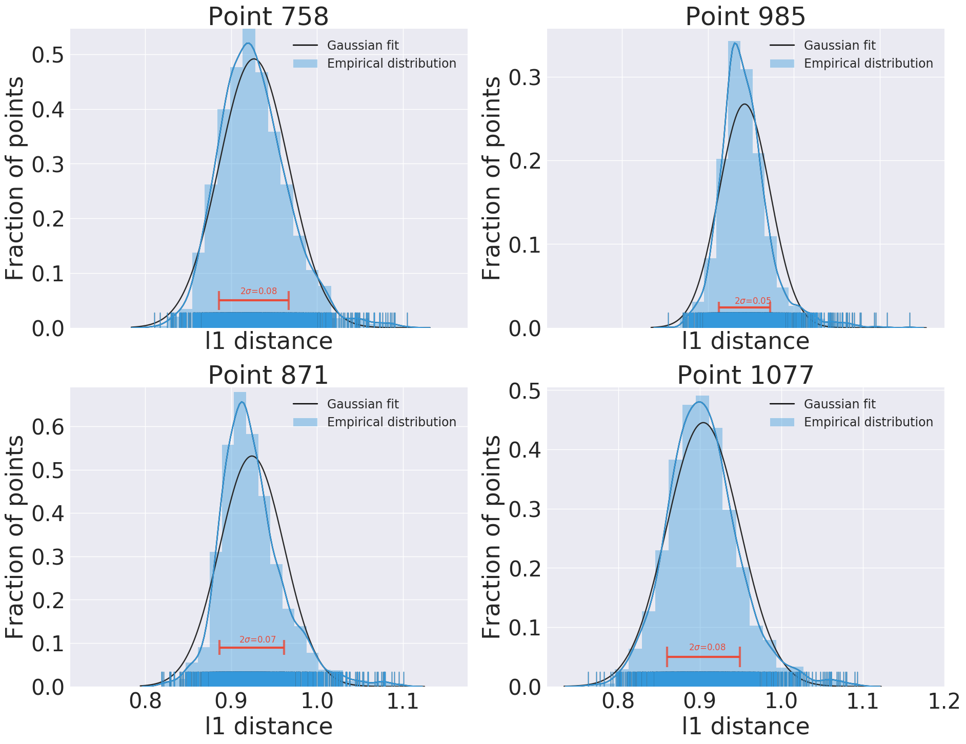
Figure 2: Histogram of $\ell_{1}$ distance of $4$ randomly chosen points (from $20,000$ points). We note that the standard deviations are around $0.05$.

2.1 The Distance Sampling Model

Example 2 suggests that for any point $x_{i}$, we can estimate its average distance $\mu_{i}$ by the empirical mean of its distance from a subset of randomly sampled points. Let us formally state this. For any point $x_{i}$, let $\mathcal{D}_{i}=\{d_{i,j},j\neq i\}$ be the set of distances associated with $x_{i}$. Define the random distance samples $D_{i,(1)},D_{i,(2)},\cdots,D_{i,(k)}$ to be i.i.d. sampled with replacement from $\mathcal{D}_{i}$. We note that

$$\mathbb{E}[D_{i,(j)}]=\mu_{i},~{}\forall i\in[n],j\in[k]$$

Hence the average distance $\mu_{i}$ can be estimated as

$$\hat{\mu}_{i}=\frac{1}{k}\sum_{i=1}^{k}D_{i,(k)}.$$

To capture the concentration property illustrated in Example 2, we assume the random variables $D_{i,(j)}$, i.e. sampling with replacement from $\mathcal{D}_{i}$, are $\sigma$-sub-Gaussian for all $i$.

2.2 Connection with Best-Arm Problem

For points whose average distance is close to that of the medoid, we need an accurate estimate of their average distance, and for points whose average distance is far away, coarse estimates suffice. Thus the problem reduces to adaptively choosing the number of distance evaluations for each point to ensure that on one hand, we have a good enough estimate of the average distance to compute the true medoid, while on the other hand, we minimise the total number of distance evaluations.

This problem has been addressed as the best-arm identification problem in the multi-armed bandit (MAB) literature (see the review article of [13] for instance). In a typical setting, we have $n$ arms. At the time $t=0,1,\cdots$, we decide to pull an arm $A_{t}\in[n]$, and receive a reward $R_{t}$ with $\mathbb{E}[R_{t}]=\mu_{A_{t}}$. The goal is to identify the arm with the largest expected reward with high probability while pulling as few arms as possible.

The medoid problem can be formulated as a best-arm problem as follows: let each point in the ensemble be an arm and let the average distance $\mu_{i}$ be the loss of the $i$-th arm. Medoid corresponds to the arm with the smallest loss, i.e the best arm. At each iteration $t$, pulling arm $i$ is equivalent to sampling (with replacement) from $\mathcal{D}_{i}$ with expected value $\mu_{i}$. As stated previosuly, the goal is to find the best arm (medoid) with as few pulls (distance computations) as possible.

3 ALGORITHM

We have $n$ points $x_{1},\cdots,x_{n}$. Recall that the average distance for arm $i$ is $\mu_{i}=\frac{1}{n-1}\sum_{j\neq i}d_{i,j}$. At iteration $t$ of the algorithm, we evaluate a distance $D_{t}$ to point $A_{t}\in[n]$. Let $T_{i}(t)$ be the number of distances of point $i$ evaluated upto time $t$. We use a variant of the Upper Confidence Bound (UCB) [17] algorithm to sample distance of a point $i$ with another point chosen uniformly at random.

We compute the empirical mean and use it as an estimate of $\mu_{i}$ at time $t$, in the initial stages of the algorithm. More concretely when $T_{i}(t)<n$,

$$\hat{\mu}_{i}(t)\triangleq\frac{1}{T_{i}(t)}\sum_{\begin{subarray}{c}1\leq\tau\leq t,A_{\tau}=i\end{subarray}}D_{\tau}.$$

Next we recall from Section 2 that the sampled distances are independent and $\sigma$-sub-Gaussian (as points are sampled with replacement). Thus for all $i$, for all $\delta\in(0,1)$, with probability at least $1-\delta$, $\mu_{i}\in[\hat{\mu}_{i}(t)-C_{i}(t),\hat{\mu}_{i}(t)+C_{i}(t)]$, where

$$C_{i}(t)=\sqrt{\frac{2\sigma^{2}\log\frac{2}{\delta}}{T_{i}(t)}}.$$ (1)

When $T_{i}(t)\geq n$, we compute the exact average distance of point $i$ and set the confidence interval to zero. Algorithm 1 describes the Med-dit algorithm.

Algorithm 1 Med-dit

1:  Evaluate distances of each point to a randomly chosen point and build a $(1-\delta)$-confidence interval for the mean distance of each point $i$: $[\hat{\mu}_{i}(1)-C_{i}(1),\ \hat{\mu}_{i}(1)+C_{i}(1)]$.

2:  while true do

3:     At iteration $t$, pick point $A_{t}$ that minimises $\hat{\mu}_{i}(t-1)-C_{i}(t-1)$.

4:     if distances of point $A_{t}$ are evaluated less than $n-1$ times then

5:        evaluate the distance of $A_{t}$ to a randomly picked point; update the confidence interval of $A_{t}$.

6:     else

7:        Set $\hat{\mu}_{i}(t)$ to be the empirical mean of distances of point $A_{t}$ by computing its distance to all $(n-1)$ other points and set $C_{A_{t}}(t)=0$.

8:     if there exists a point $x_{i^{*}}$ such that $\forall i\neq i^{*}$, $\hat{\mu}_{i^{*}}(t)+C_{i^{*}}(t)<\hat{\mu}_{i}(t)-C_{i}(t)$ then

9:        return  $x_{i^{*}}$.

Theorem 1.

For $i\in[n]$, let $\Delta_{i}=\mu_{i}-\mu^{*}$. If we pick $\delta=\frac{2}{n^{3}}$ in Algorithm 1, then with probability $1-o(1)$, it returns the true medoid with the number of distance evaluations $M$ such that,

$$M\leq\sum_{i\in[n]}\left(\frac{24\sigma^{2}}{\Delta_{i}^{2}}\log n\wedge 2n\right).$$ (2)

If $\frac{\Delta_{i}}{\sigma}$ is $\Theta(1)$, then Theorem 1 gives that Med-dit takes $O(n\log n)$ distance evaluations. In addition, if one assumed a Gaussian prior on the average distance of points (as one would expect from Figure 3), then Med-dit would also take $O(n\log n)$ distance evaluations in expectation over the prior. See Appendix 1.

If we use the same assumption as TOP-RANK, $i.e.$ the $\mu_{i}$ are i.i.d. Uniform $[c_{0},c_{1}]$, then the number of distance evaluations needed by Med-dit is $O(n^{\frac{3}{2}}\log^{\frac{1}{2}}n)$, compared to $O(n^{\frac{5}{3}}\log^{\frac{4}{3}}n)$ for TOP-RANK. Under these assumptions RAND takes $O(n^{2})$ distance evaluations to return the true medoid.

We assume that $\sigma$ is known in the proof below, whereas we estimate them in the empirical evaluations. See Section 4 for details.

Remark 1.

With a small modification to Med-dit, the sub-Gaussian assumption in Section 2 can be further relaxed to a finite variance assumption [4]. One the other hand, one could theoretically adapt Med-dit to other best-arm algorithms to find the medoid with $O(n\log\log n)$ distance computations at the sacrifice of a large constant [14]. Refer to Appendix 2 for details.

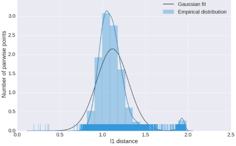
Figure 3: The distribution of mean distances of all the points in the $20,000$ cell RNA-Seq dataset.

Proof.

Let $M$ be the total number of distance evaluations when the algorithm stops. As defined above, let $T_{i}(t)$ be the number of distance evaluations of point $i$ upto time $t$.

We first assume that $[\hat{\mu}_{i}(t)-C_{i}(t),\hat{\mu}_{i}(t)-C_{i}(t)]$ are true $\left(1-\frac{2}{n^{3}}\right)$-confidence interval (Recall that $\delta=\frac{2}{n^{3}}$) and show the result. Then we prove this statement.

Let $i^{*}$ be the true medoid. We note that if we choose to update arm $i\neq i^{*}$ at time $t$, then we have

$$\hat{\mu}_{i}(t)-C_{i}(t)\leq\hat{\mu}_{i^{*}}(t)-C_{i^{*}}(t).$$

For this to occur, at least one of the following three events must occur:

$$\mathcal{E}_{1}=\left\{\hat{\mu}_{i^{*}}(t)\geq\mu_{i^{*}}(t)+C_{i^{*}}(t)\right\},$$

$$\mathcal{E}_{2}=\left\{\hat{\mu}_{i}(t)\leq\mu_{i}(t)-C_{i}(t)\right\},$$

$$\mathcal{E}_{3}=\left\{\Delta_{i}=\mu_{i}-\mu_{i^{*}}\leq 2C_{i}(t)\right\}.$$

To see this, note that if none of $\mathcal{E}_{1},\mathcal{E}_{2},\mathcal{E}_{3}$ occur, we have

$$\hat{\mu}_{i}(t)-C_{i}(t)\overset{(a)}{>}\mu_{i}-2C_{i}(t)\overset{(b)}{>}\mu_{1}\overset{(c)}{>}\hat{\mu}_{1}-C_{1}(t),$$

where $(a)$, $(b)$, and $(c)$ follow because $\mathcal{E}_{2}$, $\mathcal{E}_{3}$, and $\mathcal{E}_{1}$ do not hold respectively.

We note that as we compute $\left(1-\frac{2}{n^{3}}\right)-$confidence intervals at most $n$ times for each point. Thus we have at most $n^{2}$ computations of $\left(1-\frac{2}{n^{3}}\right)-$confidence intervals in total.

Thus $\mathcal{E}_{1}$ and $\mathcal{E}_{2}$ do not occur during any iteration with probability $1-\frac{2}{n}$, because

$$\text{w.p.}~{}(1-\frac{2}{n}):|\mu_{i}-\hat{\mu}_{i}(t)|\leq C_{i}(t),~{}\forall~{}i\in[n],~{}\forall~{}t.$$ (3)

This also implies that with probability $1-\Theta\left(\frac{1}{n}\right)$ the algorithm does not stop unless the event $\mathcal{E}_{3}$, a deterministic condition stops occurring.

Let $\zeta_{i}$ be the iteration of the algorithm when it evaluates a distance to point $i$ for the last time. From the previous discussion, we have that the algorithm stops evaluating distances to points $i$ when the following holds.

$$C_{i}(\zeta_{i})\leq\frac{\Delta_{i}}{2}\implies\frac{\Delta_{i}}{2}\geq\sqrt{\frac{2\sigma^{2}\log n^{3}}{T_{i}(\zeta_{i})}}\text{ or }C_{i}(\zeta_{i})=0,$$

$$\implies T_{i}(\zeta_{i})\geq\frac{24\sigma^{2}}{\Delta_{i}^{2}}\log n\text{ or }T_{i}(\zeta_{i})\geq 2n.$$

Thus with probability $(1-o(1))$, the algorithm returns $i^{*}$ as the medoid with at most $M$ distance evaluations, where

$$M\leq\sum_{i\in[n]}T_{i}(\zeta_{i})\leq\sum_{i\in[n]}\left(\frac{24\sigma^{2}}{\Delta_{i}^{2}}\log n\wedge 2n\right).$$

To complete the proof, we next show that $[\hat{\mu}_{i}(t)-C_{i}(t),\hat{\mu}_{i}(t)-C_{i}(t)]$ are true $\left(1-\frac{2}{n^{3}}\right)$-confidence intervals of $\mu_{i}$. We observe that if point $i$ is picked by Med-dit less than $n$ times at time t, then $T_{i}(t)$ is equal to the number of times the point is picked. Further $C_{i}(t)$ is the true $(1-\delta)$-confidence interval from Eq (1).

However, if point $i$ is picked for the $n$-th time at iteration $t$ ( line $7$ of Algorithm 1) then the empirical mean is computed by evaluating all $n-1$ distances (many distances again). Hence $T_{i}(t)=2(n-1)$. As we know the mean distance of point $i$ exactly, $C_{i}(t)=0$ is still the true confidence interval.

We remark that if a point $i$ is picked to be updated the $(n+1)$-th time, as $C_{i}(t)=0$, we have that $\forall j\neq i$,

$$\hat{\mu}_{i}(t)+C_{i}(t)=\hat{\mu}_{i}(t)-C_{i}(t)<\hat{\mu}_{j}(t)-C_{j}(t).$$

This gives us that the stopping criterion is satisfied and point $i$ is declared as the medoid.

∎

4 EMPIRICAL RESULTS

We empirically evaluate the performance of Med-dit on two real world large-scale high-dimensional datasets: the Netflix-prize dataset by [3], and 10x single cell RNA-Seq dataset [1].

We picked these large datasets because they have sparse high-dimensional feature vectors, and are at the throes of active efforts to cluster using non-Euclidean distances. In both these datasets, we use $1000$ randomly chosen points to estimate the sub-Gaussianity parameter by cross-validation. We set $\delta=1e$-$3$.

Running trimed and TOPRANK was computationally prohibitive due to the large size and high dimensionality ($\sim 20,000$) of the above two datasets. Therefore, we compare Med-dit only to RAND. We also ran Med-dit on three real world datasets tested in [24] to compare it to trimed and TOPRANK.

4.1 Single Cell RNA-Seq

Rapid advances in sequencing technology has enabled us to sequence DNA/RNA at a cell-by-cell basis and the single cell RNA-Seq datasets can contain up to a million cells [1, 16, 22, 30].

This technology involves sequencing an ensemble of single cells from a tissue, and obtaining the gene expressions corresponding to each cell. These gene expressions are subsequently used to cluster these cells in order to discover subclasses of cells which would have been hard to physically isolate and study separately. This technology therefore allows biologists to infer the diversity in a given tissue.

We note that tens of thousands gene expressions are measured in each cell, and million of cells are sequenced in each dataset. Therefore single cell RNA-Seq has presented us with a very important large-scale clustering problem with high dimensional data [30]. Moreover, the distance metric of interest here would be $\ell_{1}$ distance as the features of each point are probability distribution, Euclidean (or squared euclidean) distances do not capture the subtleties as discussed in [2, 25]. Further, very few genes are expressed by most cells and the data is thus sparse.

4.1.1 10xGenomics Mouse Dataset

We test the performance of Med-dit on the single cell RNA-Seq dataset of [1]. This dataset from 10xGenomics consists of $27,998$ genes-expression of $1.3$ million neurons cells from the cortex, hippocampus, and subventricular zone of a mice brain. These are clustered into $60$ clusters. Around $93\%$ of the gene expressions in this dataset are zero.

We test Med-dit on subsets of this dataset of two sizes:

• small dataset - $20,000$ cells (randomly chosen): We use this as we can compute the true medoid on this dataset by brute force and thus can compare the performance of Med-dit and RAND.

• large dataset - $109,140$ cells (cluster 1) is the largest cluster in this dataset. We use the most commonly returned point as the true medoid for comparision. We note that this point is the same for both Med-dit and RAND, and has the smallest distance among the top $100$ points returned in $1000$ trials of both.

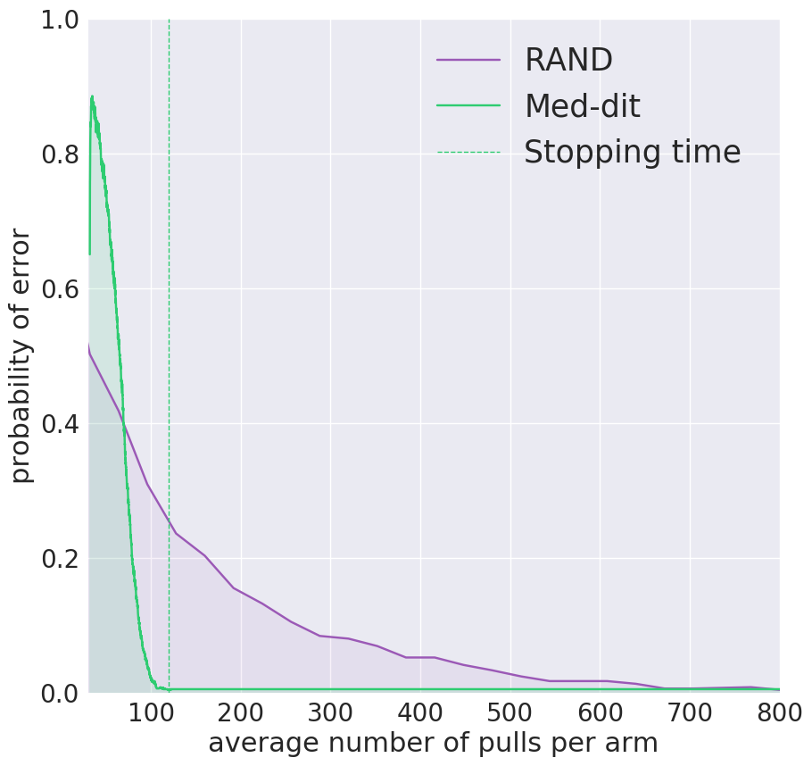
Figure 4: We computed the true medoid of the data-set by brute force. The $y$-axis shows the probability that the point with the smallest estimated mean distance is not the true medoid as a function of the number of pulls per arm. We note that Med-dit has a stopping condition while RAND does not. However we ignore the stopping condition for Med-dit here. Med-dit stops after $80$ distance evaluations per point without failing in any of the $1000$ trials, while RAND takes around $650$ distance evaluations to reach a $2\%$ probability of error.

Performance Evaluation : We compare the performance of RAND and Med-dit in Figures 1 and 4 on the large and the small dataset respectively. We note that in both cases, RAND needs $7$-$10$ times more distance evaluations to achieve $2\%$ error rate than what Med-dit stops at (without an error in $1000$ trials).

On the $20,000$ cell dataset, we note that Med-dit stopped within $140$ distance evaluations per arm in each of the $1000$ trials (with $80$ distance evaluations per arm on average) and never returned the wrong answer. RAND needs around $700$ distance evaluations per point to obtain $2\%$ error rate.

On the $109,140$ cell dataset, we note that Med-dit stopped within $140$ distance evaluations per arm in each of the $1000$ trials (with $120$ distance evaluations per arm on average) and never returned the wrong answer. RAND needs around $700$ distance evaluations per point to obtain $2\%$ error rate.

4.2 Recommendation Systems

With the explosion of e-commerce, recommending products to users has been an important avenue. Research into this took off with Netflix releasing the Netflix-prize dataset [3].

Usually in the datasets involved here, we have either rating given by users to different products (movies, books, etc), or the items bought by different users. The task at hand is to recommend products to a user based on behaviour of similar users. Thus a common approach is to cluster similar users and to use trends in a cluster to recommend products.

We note that in such datasets, we typically have the behaviour of millions of users and tens of thousands of items. Thus recommendation systems present us with an important large-scale clustering problem in high dimensions [7]. Further, most users buy (or rate) very few items on the inventory and the data is thus sparse. Moreover, the number of items bought (or rated) by users vary significantly and hence distance metrics that take this into account, like cosine distance and Jaccard distance, are of interest while clustering as discussed in [19, Chapter 9].

4.2.1 Netflix-prize Dataset

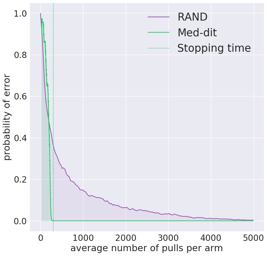
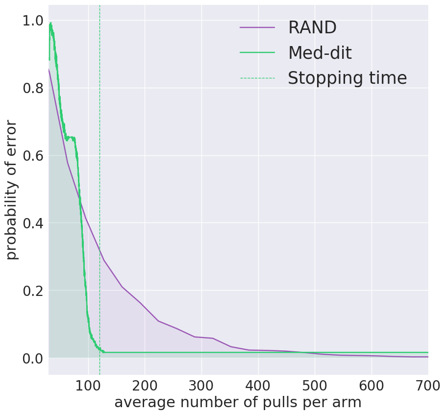
Figure 5: Left: the $20,000$ user Netflix-prize dataset. We computed the true medoid of the dataset by brute force. The $y$-axis shows the probability that the point with the smallest estimated mean distance is not the true medoid as a function of the number of pulls per arm. We note that Med-dit has a stopping condition while RAND does not. However we ignore the stopping condition for Med-dit here. Med-dit stops after $500$ distance evaluations per point without failing in any of the $1000$ trials, while RAND takes around $4500$ distance evaluations to reach a $2\%$ probability of error. Right: the $100,000$ user Netflix-prize dataset. The $y$-axis shows the probability that the point with the smallest estimated mean distance is not the true medoid as a function of the number of pulls per arm. We note that Med-dit has a stopping condition while RAND does not. However we ignore the stopping condition for Med-dit here. Med-dit stops after $500$ distance evaluations per point with $1\%$ probability of error, while RAND takes around $500$ distance evaluations to reach a $2\%$ probability of error. The computation of the true medoid here is computationally prohibitive and for comparision we use the most commonly returned point as the true medoid (which was same for both Med-dit and RAND)

We test the performance of Med-dit on the Netflix-prize dataset of [3]. This dataset from Netflix consists of ratings of $17,769$ movies by $480,000$ Netflix users. Only $0.21\%$ of the entries in the matrix are non-zero. As discussed in [19, Chapter 9], cosine distance is a popular metric considered here.

As in Section 4.1.1, we use a small and a large subset of the dataset of size $20,000$ and a $100,000$ respectively picked at random. For the former we compute the true medoid by brute force, while for the latter we use the most commonly returned point as the true medoid for comparision. We note that this point is the same for both Med-dit and RAND, and has the smallest distance among the top $100$ points returned in $1000$ trials of both.

Performance Evaluation:

On the $20,000$ user dataset (Figure 5 left), we note that Med-dit stopped within $600$ distance evaluations per arm in each of the $1000$ trials (with $500$ distance evaluations per arm on average) and never returned the wrong answer. RAND needs around $4500$ distance evaluations per point to obtain $2\%$ error rate.

On the $100,000$ users on Netflix-Prize dataset (Figure 5 right), we note that Med-dit stopped within 150 distance evaluations per arm in each of the 1000 trials (with 120 distance evaluations per arm on average) and returned the wrong answer only once. RAND needs around 500 distance evaluations per point to obtain $2\%$ error rate.

4.3 Performance on Previous Datasets

We show the performance of Med-dit on data-sets — Europe by [11] , Gnutella by [27] , MNIST by [18]— used in prior works in Table 1. The number of distance evaluations for TOPRANK and trimed are taken from [24]. We note that the performance of Med-dit on real world datasets which have low-dimensional feature vectors (like Europe) is worse than that of trimed, while it is better on datasets (like MNIST) with high-dimensional feature vectors.

We conjecture that this is due to the fact the distances in high dimensions are average of simple functions (over a each dimension) and hence have Gaussian-like behaviour due to the Central Limit Theorem (and the delta method [6]).

Dataset	$n,d$	TOPRANK	trimed	med-dit
Europe	$160k,2$	$176k$	$2862$	$3514$
Gnutella	$6.3k$, NA	$7043$	$6328$	$83$
MNIST	$6.7k,784$	$7472$	$6514$	$91$

Table 1: This table shows the performance on real-world data-sets picked from [24]. We note that performance of Med-dit on datasets, where the features are in low dimensions is not as good as that of trimed, in high dimensions Med-dit performs much better

.

4.4 Inner workings of Med-dit

Empirical running time: We computed the true mean distance $\mu_{i}$, and variance $\sigma$, for all the points in the small dataset by brute force. Figure 3 shows the histrogram of $\mu_{i}$’s. Using $\delta=1e\text{-}3$ in Theorem 1, the theoretical average number of distance evaluations is $266$. Empirically over $1000$ experiments, the average number of distance computations is $80$. This suggests that the theoretic analysis captures the essence of the algorithm.

Progress of Med-dit : We see that at any iteration of Med-dit, only the points whose lower confidence interval are smaller than the smallest upper confidence interval among all points have their distances evaluated. At any iteration, we say that such points are under consideration. We note that a point that goes out of consideration can be under consideration at a later iteration (this happens if the smallest upper confidence interval increases). We illustrate the fraction of points under consideration at different iterations (indexed by the number of distance evaluations per point) in the left panel of Figure 6. We pick $10$ snapshots of the algorithm and illustrate the true distance distributions of all points under consideration at that epoch in the right panel of Figure 6. We note that both the mean and the standard deviation of these distributions decrease as the algorithm progresses.

Confidence intervals at stopping time : Med-dit seems to compute the mean distance of a few points exactly. These are usually points with the mean distance close to the that of the medoid. The points whose mean distances are farther away from that of the medoid have fewer distances evaluated to have the confidence intervals rule them out as the medoid. The $99.99\%$ confidence interval of the top $150$ points in a run of the experiment are shown in Figure 7 for the $20,000$ cell RNA-Seq dataset. This allows the algorithm to save on distance computations while returning the correct answer.

Speed-accuracy tradeoff Setting the value of $\delta$ between $0.01$ to $0.1$ will result in smaller confidence intervals around the estimates $\hat{\mu}_{i}$, which will ergo reduce the number of distance evaluations. One could also run Med-dit for a fixed number of iterations and return the point with the smallest mean estimate. Both of these methods improve the running time at the cost of accuracy. Practically, the first method has a better trade-off between accuracy and running time whereas the second method has a deterministic stopping time.

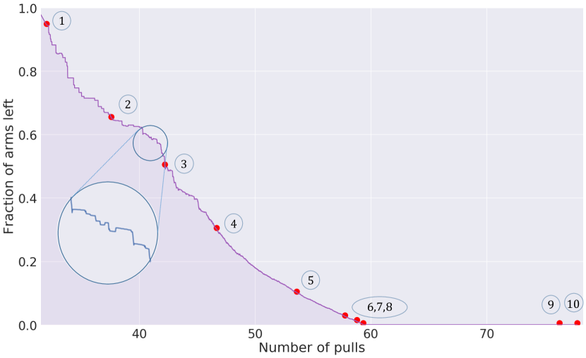
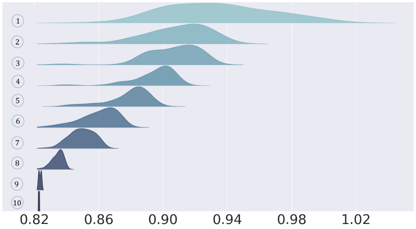
Figure 6: In the left panel, we show the number of points under consideration at different iterations in Med-dit. We note that though the number of points under consideration show a decreasing trend, they do not decrease monotonically. In the right panel, we show the distribution of the true distances among the arms that are under consideration at various snapshots of the algorithm. We note that both the mean and the variance of the distributions keeps decreasing. The last snapshot shows only the distance of the point declared a medoid.

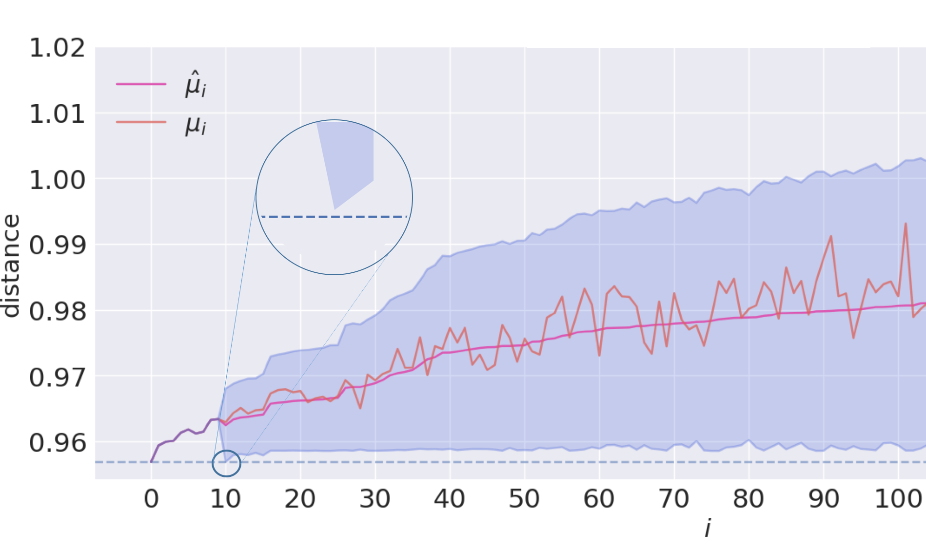
Figure 7: $99.99\%$-Confidence Intervals of the $150$ points with smallest estimated mean distance in the $20,000$ cell dataset at the termination of Med-dit. The true means are shown by the orange line, while the estimated means are shown by the pink line. We note that the distances of $9$ points are computed to all other points. We also note that mean of the medoid is less than the $99.99\%$-lower confidence bound of all the other points.

Appendices

1 The $O(n\log n)$ Distance Evaluations Under Gaussian Prior

We assume that the mean distances of each point $\mu_{i}$ are i.i.d. samples of ${N}(\gamma,1)$. We note that this implies that $\Delta_{i},\ 1\leq i\leq n$ are $n$ iid random variables. Let $\Delta$ be a random variable with the same law as $\Delta_{i}$.

From the concentration of the minimum of $n$ gaussians, we have that

$$\min_{i}\mu_{i}+\sqrt{2\log n}\overset{p}{\rightarrow}\gamma.$$

This gives us that

$$\Delta-\sqrt{2\log n}\overset{d}{\rightarrow}\mathcal{N}(0,1).$$

We note that by Eq (2), we have that the expected number of distance evaluations $M$ is of the order of

$$\mathbb{E}[M] \leq n\mathbb{E}\left[\frac{\log n}{\Delta^{2}}\wedge n\right],$$

where the expection is taken with respect to the randomness of $\Delta$.

To show this, it is enough to show that,

$$\mathbb{E}\left[\frac{\log n}{\Delta^{2}}\wedge n\right]\leq C\log n,$$

for some constant $C$.

To compute that for this prior, we divide the real line into three intervals, namely

• $\left(-\infty,\sqrt{\frac{{\log n}}{n}}\right]$,

• $\left(\sqrt{\frac{{\log n}}{n}},c\sqrt{\log n}\right)$,

• $\left[c\sqrt{\log n},\infty\right)$,

and compute the expectation on these three ranges. We note that for if $\Delta\in(-\infty,\sqrt{\frac{{\log n}}{n}}]$, while for $\Delta\in(\sqrt{\frac{{\log n}}{n}},\infty]$, $\frac{\log n}{\Delta^{2}}\leq n$. Thus we have that,

$$\mathbb{E}\left[\frac{\log n}{\Delta^{2}}\wedge n\right] \leq\overbrace{\mathbb{E}\left[n\mathbb{I}\left(\Delta\leq\sqrt{\frac{{\log n}}{n}}\right)\right]}^{\mathbf{I}}+\overbrace{\lim_{\delta,\epsilon\rightarrow 0}\mathbb{E}\left[\frac{\log n}{\Delta^{2}}\mathbb{I}\left(\sqrt{\frac{\log n}{n^{(1-\epsilon)}}}\leq\Delta\leq c\frac{\sqrt{\log n}}{n^{\delta}}\right)\right]}^{\mathbf{II}}$$

$$\quad\quad+\underbrace{\mathbb{E}\left[\frac{\log n}{\Delta^{2}}\mathbb{I}\left(\Delta\geq c\sqrt{\log n}\right)\right]}_{\mathbf{III}},$$

where we use the Bounded Convergence Theorem to establish $\mathbf{II}$.

We next show that all three terms in the above equation are of $O(\log n)$. We first show the easy cases of $\mathbf{I}$ and $\mathbf{III}$ and then proceed to $\mathbf{III}$.

• To establish that $\mathbf{I}$ is $O(\log n)$, we start by defining, $q_{1}=P[\Delta<\frac{\sqrt{\log n}}{n}]$

  $$\mathbb{E}\left[n\mathbb{I}\left(\Delta\leq\frac{\sqrt{\log n}}{n}\right)\right] =nq_{1}.$$

  Further note that,

  $$q_{1} \leq\exp\left(-\frac{1}{2}\left(\sqrt{2\log n}-\sqrt{\frac{\log n}{n}}\right)^{2}\right),$$

  $$=\left(\frac{1}{n}\right)^{(1-\frac{1}{\sqrt{2n}})^{2}}.$$

  Thus

  $$\frac{q_{1}n}{\log n} \leq\frac{n^{1-(1-\frac{1}{\sqrt{2n}})^{2}}}{\log n},$$

  $$\leq\exp((\sqrt{\frac{2}{n}}(1+o(1))\log n-\log\log n),$$

  $$=o(1).$$

• To establish that $\mathbf{III}$ is $O(\log n)$, we note that,

  $$\mathbb{E}\left[\frac{\log n}{\Delta^{2}}\mathbb{I}\left(\Delta\geq c\sqrt{\log n}\right)\right] \leq\frac{1}{c^{2}}P(\Delta\geq c\sqrt{\log n}),$$

  $$\leq\frac{1}{c^{2}},$$

  $$=\Theta(1).$$

• Finally to establish that $\mathbf{II}$ is $O(\log n)$, we note that,

  $$\lim_{\delta,\epsilon\rightarrow 0}\mathbb{E}\left[\frac{\log n}{\Delta^{2}}\mathbb{I}\left(\sqrt{\frac{\log n}{n^{(1-\epsilon)}}}\leq\Delta\leq c\frac{\sqrt{\log n}}{n^{\delta}}\right)\right] \leq\lim_{\delta,\epsilon\rightarrow 0}n^{2-\epsilon}P\left(\Delta\leq c\frac{\sqrt{\log n}}{n^{\delta}}\right),$$

  $$\leq\lim_{\delta,\epsilon\rightarrow 0}n^{1-\epsilon}\exp\left(-\frac{1}{2}\left(\sqrt{2\log n}-\sqrt{\log n}\frac{c}{n^{\delta}}\right)^{2}\right),$$

  $$=\lim_{\delta,\epsilon\rightarrow 0}n^{1-\epsilon}\left(\frac{1}{n}\right)^{(1-\frac{c}{\sqrt{2}n^{\delta}})^{2}},$$

  $$=\lim_{\delta,\epsilon\rightarrow 0}n^{1-\epsilon-(1-\frac{c}{\sqrt{2}n^{\delta}})^{2}},$$

  $$=\lim_{\delta,\epsilon\rightarrow 0}n^{-\epsilon+\frac{\sqrt{2}c}{n^{\delta}}-\frac{c^{2}}{2n^{2\delta}}}.$$

  Letting $\delta$ to go to $0$ faster than $\epsilon$, we see that,

  $$\lim_{\delta,\epsilon\rightarrow 0}\mathbb{E}\left[\frac{\log n}{\Delta^{2}}\mathbb{I}\left(\sqrt{\frac{\log n}{n^{(1-\epsilon)}}}\leq\Delta\leq c\frac{\sqrt{\log n}}{n^{\delta}}\right)\right] \leq O(\log n).$$

This gives us that under this model, we have that under this model,

$$\mathbb{E}[M]\leq O(n\log n).$$

2 Extensions to the Theoretical Results

In this section we discuss two extensions to the theoretical results presented in the main article:

1. relax the sub-Gaussian assumption used for the analysis of Med-dit. We see that assuming that the distances random variables have finite variances is enough for a variant of Med-dit to need essentially the same number of distance evaluations as Theorem 1. The variant would use a different estimator (called Catoni’s M-estimator [5]) for the mean distance of each point instead of empirical average leveraging the work of [4]. This is based on the work of [4].

2. note that there exists an algorithm which can compute the medoid with $O(n\log\log n)$ distance evaluations. The algorithm called exponential-gap algorithm [14] and is discussed below.

2.1 Weakening the Sub-Gaussian Assumption

We note that in order to have the $O(n\log n)$ sample complexity, Med-dit relies on a concentration bound where the tail probability decays exponentially. This is achieved by assuming that for each point $x_{i}$, the random variable of sampling with replacement from $\mathcal{D}_{i}$ is $\sigma$-sub-Gaussian in Theorem 1. As a result, we can have the sub-Gaussian tail bound that for any point $x_{i}$ at time $t$, with probability at least $1-\delta$, the empirical mean $\hat{\mu}_{i}$ satisfies

$$|\mu_{i}-\hat{\mu}_{i}|\leq\sqrt{\frac{2\sigma^{2}\log\frac{2}{\delta}}{T_{i}(t)}}.$$

In fact, as pointed out by [4], to achieve the $O(n\log n)$ sample complexity, all we need is a performance guarantee like the one shown above for the empirical mean. To be more precise, we need the following property:

Assumption 1.

[4] Let $\epsilon\in(0,1]$ be a positive parameter and let $c,v$ be positive constants. Let $X_{1},\cdots,X_{T}$ be i.i.d. random variables with finite mean $\mu$. Suppose that for all $\delta\in(0,1)$, there exists an estimator $\hat{\mu}=\hat{\mu}(T,\delta)$ such that, with probability at least $1-\delta$,

$$|\mu-\hat{\mu}|\leq v^{\frac{1}{1+\epsilon}}\left(\frac{c\log\frac{2}{\delta}}{T}\right)^{\frac{\epsilon}{1+\epsilon}}.$$

Remark 2.

If the distribution of $X_{j}$ satisfies $\sigma$-sub-Gaussian condition, then Assumption 1 is satisfied for $\epsilon=1$, $c=2$, and variance factor $v=\sigma^{2}$.

However, Assumption 1 can be satisfied with conditions much weaker than the sub-Gaussian condition. One way is by substituing the empirical mean estimator by some refined mean estimator that gives the exponential tail bound. Specifically, as suggested by [4], we can use Catoni’s M-estimator [5].

Catoni’s M-estimator is defined as follows: let $\psi:\mathbb{R}\to\mathbb{R}$ be a continuous strictly increasing function satisfying

$$-\log(1-x+\frac{x^{2}}{2})\leq\psi(x)\leq\log(1+x+\frac{x^{2}}{2}).$$

Let $\delta\in(0,1)$ be such that $T>2\log(\frac{1}{\delta})$ and introduce

$$\alpha_{\delta}=\sqrt{\frac{2\log\frac{1}{\delta}}{T(\sigma^{2}+\frac{2\sigma^{2}\log\frac{1}{\delta}}{T-2\log\frac{1}{\delta}})}}.$$

If $X_{1},\cdots,X_{T}$ are i.i.d. random variables, the Catoni’s estimator is defined as the unique value $\hat{\mu}_{C}=\hat{\mu}_{C}(T,\delta)$ such that

$$\sum_{i=1}^{n}\psi(\alpha_{\delta}(X_{i}-\hat{\mu}_{C}))=0.$$

Catoni [5] proved that if $T\geq 4\log\frac{1}{\delta}$ and the $X_{j}$ have mean $\mu$ and variance at most $\sigma^{2}$, then with probability at least $1-\delta$,

$$|\hat{\mu}_{C}-\mu|\leq 2\sqrt{\frac{\sigma^{2}\log\frac{2}{\delta}}{T}}.$$ (4)

The corresponding modification to Med-dit is as follows.

1. For the initialization step, sample each point $4\log\frac{1}{\delta}$ times to meet the condition for the concentration bound of the Catoni’s M-estimator.

2. For each arm $i$, if $T_{i}(t)<n$, maintain the $1-\delta$ confidence interval $[\hat{\mu}_{C,i}-C_{i}(t),\hat{\mu}_{C,i}+C_{i}(t)]$, where $\hat{\mu}_{C,i}$ is the Catoni’s estimator of $\mu_{i}$, and

   $$C_{i}(t)=2\sqrt{\frac{\sigma^{2}\log\frac{2}{\delta}}{T_{i}(t)}}.$$

Proposition 1.

For $i\in[n]$, let $\Delta_{i}=\mu_{i}-\mu^{*}$. If we pick $\delta=\frac{1}{n^{3}}$ in the above algorithm, then with probability $1-o(1)$, it returns the true medoid with the with number of distance evaluations $M$ such that,

$$M\leq 12n\log n+\sum_{i\in[n]}\left(\frac{48\sigma^{2}}{\Delta_{i}^{2}}\log n\wedge 2n\right)$$

Proof.

Let $\delta=\frac{2}{n^{3}}$. The initialization step takes an extra $12n\log n$ distance computations. Following the same proof as Theorem 1, we can show that the modified algorithm returns the true medoid with probability at least $1-\Theta(\frac{1}{n})$, and apart from the initialization, the total number of distance computations can be upper bounded by

$$\sum_{i\in[n]}\left(\frac{48\sigma^{2}}{\Delta_{i}^{2}}\log n\wedge 2n\right).$$

So the total number of distance computations can be upper bounded by

$$M\leq 12n\log n+\sum_{i\in[n]}\left(\frac{48\sigma^{2}}{\Delta_{i}^{2}}\log n\wedge 2n\right).$$

∎

Remark 3.

By using the Catoni’s estimator, instead of the empirical mean, we need a much weaker assumption that the distance evaluations have finite variance to get the same results as Theorem 1.

2.2 On the $O(n\log\log n)$ Algorithm

The best-arm algrithm exponential-gap [14] can be directly applied on the medoid problem, which takes $O(\sum_{i\neq i^{*}}\Delta_{i}^{-2}\log\log\Delta_{i}^{-2})$ distance evaluations, essentially $O(n\log\log n)$ if $\Delta_{i}$ are constants. It is an variation of the familiy of action elimination algorithm for the best-arm problem. A typical action elimination algorithm proceeds as follows: Maintaining a set $\Omega_{k}$ for $k=1,2,\cdots$, initialized as $\Omega_{1}=[n]$. Then it proceeds in epoches by sampling the arms in $\Omega_{k}$ a predetermined number of times $r_{k}$, and maintains arms according to the rule:

$$\Omega_{k+1}=\{i\in\Omega_{k}:\hat{\mu}_{a}+C_{a}(t)<\hat{\mu}_{i}-C_{i}(t)\},$$

where $a\in\Omega_{k}$ is a reference arm, e.g. the arm with the smallest $\hat{\mu}_{i}+C_{i}(t)$. Then the algorithm terminates when $\Omega_{k}$ contains only one element.

The above vanilla version of the action elimination algorithm takes $O(n\log n)$ distance evaluations, same as Med-dit. The improvement by exponential-gap is by observing that the suboptimal $\log n$ factor is due to the large deviations of $|\hat{\mu}_{a}-\mu_{a}|$ with $a=\arg\min_{i\in\Omega_{k}}\hat{\mu}_{i}$. Instead, exponential-gap use a subroutine median elimination [10] to determine an alternative reference arm $a$ with smaller deviations and allows for the removal of the $\log n$ term, where median elimination takes $O(\frac{n}{\epsilon^{2}}\log\frac{1}{\delta})$ distance evaluations to return a $\epsilon$-optimal arm. However, this will introduce a prohibitively large constant due to the use of median elimination. Regarding the technical details, we note both paper [14, 10] assume the boundedness of the random variables for their proof, which is only used to have the hoefflding concentration bound. Therefore, with our sub-Gaussian assumption, the proof will follow symbol by symbol, line by line.

References

- [1] 10xGenomics. 1.3 Million Brain Cells from E18 Mice. 10x Genomics, 2017. available at https://support.10xgenomics.com/single-cell-gene-expression/datasets/1M_neurons.
- [2] Tugkan Batu, Lance Fortnow, Ronitt Rubinfeld, Warren D Smith, and Patrick White. Testing that distributions are close. In Foundations of Computer Science, 2000. Proceedings. 41st Annual Symposium on, pages 259–269. IEEE, 2000.
- [3] James Bennett, Stan Lanning, et al. The netflix prize. In Proceedings of KDD cup and workshop, volume 2007, page 35. New York, NY, USA, 2007.
- [4] Sébastien Bubeck, Nicolo Cesa-Bianchi, and Gábor Lugosi. Bandits with heavy tail. IEEE Transactions on Information Theory, 59(11):7711–7717, 2013.
- [5] Olivier Catoni et al. Challenging the empirical mean and empirical variance: a deviation study. In Annales de l’Institut Henri Poincaré, Probabilités et Statistiques, volume 48, pages 1148–1185. Institut Henri Poincaré, 2012.
- [6] Aad W Chapter 3 Van der Vaart. Asymptotic statistics, volume 3. Cambridge university press, 1998.
- [7] Srivatsava Daruru, Nena M Marin, Matt Walker, and Joydeep Ghosh. Pervasive parallelism in data mining: dataflow solution to co-clustering large and sparse netflix data. In Proceedings of the 15th ACM SIGKDD international conference on Knowledge discovery and data mining, pages 1115–1124. ACM, 2009.
- [8] David Eppstein and Joseph Wang. Fast approximation of centrality. Graph Algorithms and Applications 5, 5:39, 2006.
- [9] Eyal Even-Dar, Shie Mannor, and Yishay Mansour. Pac bounds for multi-armed bandit and markov decision processes. In International Conference on Computational Learning Theory, pages 255–270. Springer, 2002.
- [10] Eyal Even-Dar, Shie Mannor, and Yishay Mansour. Action elimination and stopping conditions for the multi-armed bandit and reinforcement learning problems. Journal of machine learning research, 7(Jun):1079–1105, 2006.
- [11] P. Fränti, M. Rezaei, and Q. Zhao. Centroid index: cluster level similarity measure. Pattern Recognition, 47(9):3034–3045, 2014.
- [12] Charles AR Hoare. Algorithm 65: find. Communications of the ACM, 4(7):321–322, 1961.
- [13] Kevin Jamieson and Robert Nowak. Best-arm identification algorithms for multi-armed bandits in the fixed confidence setting. In Information Sciences and Systems (CISS), 2014 48th Annual Conference on, pages 1–6. IEEE, 2014.
- [14] Zohar Karnin, Tomer Koren, and Oren Somekh. Almost optimal exploration in multi-armed bandits. In Proceedings of the 30th International Conference on Machine Learning (ICML-13), pages 1238–1246, 2013.
- [15] Leonard Kaufman and Peter Rousseeuw. Clustering by means of medoids. North-Holland, 1987.
- [16] Allon M Klein, Linas Mazutis, Ilke Akartuna, Naren Tallapragada, Adrian Veres, Victor Li, Leonid Peshkin, David A Weitz, and Marc W Kirschner. Droplet barcoding for single-cell transcriptomics applied to embryonic stem cells. Cell, 161(5):1187–1201, 2015.
- [17] Tze Leung Lai and Herbert Robbins. Asymptotically efficient adaptive allocation rules. Advances in applied mathematics, 6(1):4–22, 1985.
- [18] Yann LeCun. The mnist database of handwritten digits. http://yann. lecun. com/exdb/mnist/, 1998.
- [19] Jure Leskovec, Anand Rajaraman, and Jeffrey David Ullman. Mining of massive datasets. Cambridge university press, 2014.
- [20] George C Linderman and Stefan Steinerberger. Clustering with t-sne, provably. arXiv preprint arXiv:1706.02582, 2017.
- [21] Stuart Lloyd. Least squares quantization in pcm. IEEE transactions on information theory, 28(2):129–137, 1982.
- [22] Evan Z Macosko, Anindita Basu, Rahul Satija, James Nemesh, Karthik Shekhar, Melissa Goldman, Itay Tirosh, Allison R Bialas, Nolan Kamitaki, Emily M Martersteck, et al. Highly parallel genome-wide expression profiling of individual cells using nanoliter droplets. Cell, 161(5):1202–1214, 2015.
- [23] James MacQueen et al. Some methods for classification and analysis of multivariate observations. In Proceedings of the fifth Berkeley symposium on mathematical statistics and probability, volume 1, pages 281–297. Oakland, CA, USA., 1967.
- [24] James Newling and François Fleuret. A sub-quadratic exact medoid algorithm. Proceedings of the 20th International Conference on Artificial Intelligence and Statistics, 2017.
- [25] Vasilis Ntranos, Govinda M Kamath, Jesse M Zhang, Lior Pachter, and David N Tse. Fast and accurate single-cell rna-seq analysis by clustering of transcript-compatibility counts. Genome biology, 17(1):112, 2016.
- [26] Kazuya Okamoto, Wei Chen, and Xiang-Yang Li. Ranking of closeness centrality for large-scale social networks. In International Workshop on Frontiers in Algorithmics, pages 186–195. Springer, 2008.
- [27] Matei Ripeanu, Ian Foster, and Adriana Iamnitchi. Mapping the gnutella network: Properties of large-scale peer-to-peer systems and implications for system design. arXiv preprint cs/0209028, 2002.
- [28] Hugo Steinhaus. Sur la division des corp materiels en parties. Bull. Acad. Polon. Sci, 1(804):801, 1956.
- [29] Cathie Sudlow, John Gallacher, Naomi Allen, Valerie Beral, Paul Burton, John Danesh, Paul Downey, Paul Elliott, Jane Green, Martin Landray, et al. Uk biobank: an open access resource for identifying the causes of a wide range of complex diseases of middle and old age. PLoS medicine, 12(3):e1001779, 2015.
- [30] Grace XY Zheng, Jessica M Terry, Phillip Belgrader, Paul Ryvkin, Zachary W Bent, Ryan Wilson, Solongo B Ziraldo, Tobias D Wheeler, Geoff P McDermott, Junjie Zhu, et al. Massively parallel digital transcriptional profiling of single cells. Nature communications, 8:14049, 2017.