A VST and VISTA study of globular clusters in NGC 253

Abstract

Context. Globular clusters (GCs) are key to our understanding of the Universe, as laboratories of stellar evolution, fossil tracers of the past formation epoch of the host galaxy, and effective distance indicators from local to cosmological scales.

Aims. We analyze the properties of the sources in the NGC 253 with the aim of defining an up to date catalog of GC candidates in the galaxy. Given the distance of the galaxy, GCs in NGC 253 are ideal targets for resolved color-magnitude diagram studies of extragalactic GCs with next-generation diffraction limited ground-based telescopes.

Methods. Our analysis is based on the science verification data of two ESO survey telescopes, VST and VISTA. Using $ugri$ photometry from VST and $JK_{s}$ from VISTA, GC candidates were selected using as reference the morpho-photometric and color properties of spectroscopically confirmed GCs available in the literature. The strength of the results was verified against available archival HST/ACS data from the GHOSTS survey: all but two of the selected GC candidates appear as star clusters in HST footprints.

Results. The adopted GC selection leads to the definition of a sample of $\sim 350$ GC candidates. At visual inspection, we find that 82 objects match all the requirements for selecting GC candidates and 155 are flagged as uncertain GC candidate; however, 110 are unlikely GCs, which are most likely background galaxies. Furthermore, our analysis shows that four of the previously spectroscopically confirmed GCs, i.e., $\sim 20\%$ of the total spectroscopic sample, are more likely either background galaxies or high-velocity Milky Way stars. The radial density profile of the selected best candidates shows the typically observed $r^{1/4}$-law radial profile. The analysis of the color distributions reveals only marginal evidence of the presence of color bimodality, which is normally observed in galaxies of similar luminosity. The GC luminosity function does not show the typical symmetry, mainly because of the lack of bright GCs. Part of the bright GCs missing might be at very large galactocentric distances or along the line of sight of the galaxy dusty disk. As an alternative possibility, we speculate that a fraction of low luminosity GC candidates might instead be metal-rich, intermediate age clusters, but fall in a similar color interval of old, metal-poor GCs.

Conclusions. Defining a contaminant-free sample of GCs in extragalactic systems is not a straight forward exercise. Using optical and near-IR photometry we purged the list of GCs with spectroscopic membership and photometric GC candidates in NGC 253. Our results show that the use of either spectroscopic or photometric data only does not generally ensure a contaminant-free sample and a combination of both spectroscopy and photometry is preferred.

1 Introduction

Globular clusters (GCs) are a key tool for understanding the formation and evolution of galaxies (Harris, 2001; Brodie & Strader, 2006; Peng et al., 2008; Georgiev et al., 2010; Harris et al., 2013; Durrell et al., 2014).

Extragalactic, unresolved GCs are possibly the simplest class of astrophysical objects beyond stars as, to a first approximation, they host a simple, single age and single metallicity, stellar population. Nevertheless, in the last decade such a classical paradigm has been demonstrated as invalid for a fraction of Milky Way (MW) GCs and for some of the clusters in the Magellanic Clouds (Gratton et al., 2004; Piotto et al., 2007; Carretta et al., 2009). In spite of that, doubtless GCs are the simplest stellar aggregates to be found in galaxies.

Two other properties make GCs very useful for extragalactic studies: old age and high luminosity. In the few galaxies, beyond the MW, where spectroscopic or multiband photometric studies of the GCs have been carried out, the results almost uniformly revealed a population with mean ages comparable to the GC system of the MW, older than $\sim$10 Gyr (e.g., Cohen et al., 1998, 2003; Strader et al., 2005; Chies-Santos et al., 2011). This makes GCs fossil tracers of the formation of the host galaxy. In addition, extragalactic GCs appear as bright clumps of light on the otherwise smooth light profile of the galaxy and, under typical observing conditions from the ground, they appear as point-like sources.

The compactness and high contrast with respect to the background light from galaxy and sky, make GCs observable out to large distances. Photometric studies with the Hubble Space Telescope (HST) have been carried out for GC systems at $z\sim 0.2$ ($d\sim 800$ Mpc, ACS data, Alamo-Martínez et al., 2013) and at $z\sim 0.3$ ($d\sim 1250$ Mpc, ACS and WFC3 data, Janssens et al., 2017). Furthermore, very recently Vanzella et al. (2017) have reported the discovery of several compact extremely young objects at redshift $z>3$, observed with Very Large Telescope/Multi Unit Spectroscopic Explorer (VLT/MUSE), some of which have inferred physical properties consistent with those expected in proto-GCs.

Beyond their role as laboratories for the validation and calibration of stellar evolution from the data of the closest resolved GCs (Salaris & Cassisi, 2005), the systematic study of extragalactic GC systems has revealed a wealth of properties used to trace the physical characteristics of the GC system and the host galaxy; for example, the luminosity function of GCs (GCLF), spatial distribution, projected surface density, radial color profiles, specific frequency, kinematical properties, and color-magnitude relations are effective tracers of the past formation and evolution history of the galaxy, its physical distance, possible merging events, mass distribution, etc. (Harris, 2001; Brodie & Strader, 2006).

Studies of extragalactic GCs based on photometry are hampered by a varying level of contamination from foreground MW stars and background galaxies. On the other hand, spectroscopic observations can provide cleaner GC samples, but they are feasible only for the nearest, brightest GC systems, even with the largest 8-10 m class telescopes (Brodie et al., 2014).

In this paper we use the science verification imaging data in the $ugriJK_{s}$ bands, taken with the VST and VISTA ESO survey telescopes, to obtain an updated catalog of GCs in NGC 253, thereby taking advantage of the large wavelength range covered.

The galaxy, the brightest in the Sculptor group (Karachentsev et al., 2003), at a distance of $\sim 3.5$ Mpc (Radburn-Smith et al., 2011), is an edge-on disk galaxy and, together with M 82, is one of the two brightest, closest starburst galaxies (McCarthy et al., 1987). Two different spectroscopic studies, by Beasley & Sharples (2000) and by Olsen et al. (2004), have targeted the GC system of the galaxy, leading to a total of 21 spectroscopically confirmed GCs, which we use as reference sample. Other photometric studies exist in the literature (Liller & Alcaino, 1983; Blecha, 1986). The advantage of the catalog we present in this work is the wider wavelength coverage and larger angular coverage of the data analyzed. Galleti et al. (2004) announced 380 globular cluster candidates in NGC 253 selected with photometric data. The follow-up study based on VIMOS/VLT spectroscopic data is still unpublished. In general, both spectroscopic and photometric studies of GCs in the Sculptor group are consistent with low metallicity, $[Fe/H]$ $\ \raise-2.0pt\hbox{\hbox to0.0pt{\hbox{$\sim$}\hss}\raise 5.0pt\hbox{$<$}\ }-1$, and with a cumulative luminosity function (LF) consistent with the Milky Way. However, for NGC 253, the conclusions are tempered by the small sample size of confirmed GCs and by the large contamination in photometric samples. We aim to remedy that by using VST and VISTA high-resolution multiwavelength imaging data.

The paper is organized as follows: The next section describes the observations, procedures for data reduction and for deriving the photometry of the sources in the optical and near-IR frames. The selection of GCs candidates is described in Section 3. Section 4 provides the final catalog and a brief discussion of our results. A summary of the main results closes the paper.

2 Observations, data reduction, and analysis

The data presented in this paper were collected as part of science verification of VST (Iodice et al., 2012) and VISTA (Arnaboldi et al., 2010, 2012). In particular we analyzed the $ugri$ data from VST and the $JK_{s}$ from VISTA.

The VST data were processed with VST-Tube (Grado et al., 2012), a pipeline specialized for the data reduction of VST-OmegaCAM executing prereduction (bias subtraction and flat normalization), illumination and (for the $i$ band) fringe corrections, and photometric and astrometric calibration.

The data reduction for VISTA was carried out with the VISTA data flow system at the Cambridge Astronomy Survey Unit (see Irwin et al., 2004; Greggio et al., 2014; Iodice et al., 2014, for more details).

A summary of the observations is provided in Table 1, together with a list of properties of the target galaxy. The final image size was $\sim 1.04^{\circ}\times 1.09^{\circ}$ for VST at $0.21\arcsec/pixel$ resolution with the $ugri$ pointings centered on the galaxy. For VISTA, the image size was $\sim 1.2^{\circ}\times 1.5^{\circ}$, at $0.339\arcsec/pixel$ resolution centered at R.A.=00:46:59 and Dec.=-25:17:26 with the photometric center of the galaxy slightly offset eastward of the pointing center. Figure 1 and Figure 2 show the full field of view observed by VST and VISTA in $g$ and $J$ band, respectively. The final combined field of view is of $\sim 1.05\deg^{2}$, over which we have photometry in all six bands.

We need to minimize contamination due to the light from the galaxy to study GCs. To model and subtract the surface brightness profile of NGC 253, we used the ISOPHOTE/ELLIPSE task in IRAF/STSDAS (Jedrzejewski, 1987). The geometric parameters of the galaxy light fits are on average position angle $\sim 51\deg$ and ellipticity $\sim 0.78$ in all inspected bands, which is consistent with previous results (Iodice et al., 2014).

After modeling and subtracting the profile of the galaxy, to produce a complete catalog of all sources in the VST and VISTA field of view, we independently ran SExtractor (Bertin & Arnouts, 1996) on the galaxy-model-subtracted frame for each filter. We obtained aperture magnitudes within a diameter aperture of eight pixels ($\sim 1\aas@@fstack{\prime\prime}7$ at OmegaCAM/VST resolution and $\sim 2\aas@@fstack{\prime\prime}7$ for the VIRCAM/VISTA), and applied aperture correction to infinite radius. The aperture correction is derived from the analysis of the curve of growth of bright isolated point-like sources. The aperture correction terms derived are $ap.corr.$=0.43, 0.38, 0.40, 0.25, 0.19, 0.14 mag in $u$, $g$, $r$, $i$, $J$, $K_{s}$, respectively, with typical uncertainty of $\sim 0.01$ mag. We assumed constant Galactic extinction on the frames with the Schlafly & Finkbeiner (2011) recalibration of the Schlegel et al. (1998) infrared-based dust maps.

The VST images are calibrated in the SDSS photometric system using several Landolt (1992) standard fields with calibrated SDSS photometry. VISTA is instead calibrated against 2MASS photometry. We independently verified the calibrations by comparing the $ugri$ magnitudes with $\sim 500$ objects with photometry available from APASS. For the $u$, $g,$ and $r$ bands the median difference between our VST and APASS magnitudes is $\leq$0.04 mag, which is smaller than the $rms$ scatter in every case. For the $i$ band, we found a small color independent offset of $\sim 0.1$ mag that is still consistent with zero within the estimated $rms$ ($\langle m_{i}^{VST}-m_{i}^{APASS}\rangle=0.10\pm 0.11$ mag). The same behavior of VST and APASS photometry in $i$ band was also found on completely different targets, from the Fornax Deep Survey (Iodice et al., 2016; D’Abrusco et al., 2016; Cantiello et al., 2017) and with a data reduction tool independent from VST-Tube (i.e., with AstroWise; Aku Venhola, priv. communication). Furthermore, the comparison of $i$-band photometry for VST data with data in the literature for other targets in the VEGAS survey (e.g., NGC 3115; Cantiello et al., 2015) did not show any peculiar offset in this band. Hence, our conclusion is that a small difference exists in the system throughput and image quality at $i$-band wavelengths between the two telescope-instrument combinations, leading to the observed increased offset and scatter.

For the near-IR bands, we checked the photometry with an independent comparison to 2MASS point sources photometry. The agreement is satisfactory for both bands with an offset $\leq 0.04$ mag and $rms$ nearly twice as large.

The photometric catalogs in the six bands were matched adopting $1\aas@@fstack{\prime\prime}2/1\aas@@fstack{\prime\prime}4$ matching radius for VST/VISTA. The full catalog of $\sim 1.200.000$ sources is available on the VEGAS project web-page and on the CDS archive. Sources with matched photometry in all six bands, or with missing detections in one or more filters, are included in the full catalog.

A color magnitude diagram and some color-color diagrams of the full matched catalog are shown in Figure 3. In the figure, we show separately the $\sim 70.000$ sources detected in areas with high and highly variable galaxy backgrounds (i.e., in regions where $\mu_{g}\leq 23.6\leavevmode\nobreak\ mag/arcsec^{2}$, left panels) and those detected where the galaxy background is negligible (right panels).

Table 1: Properties of the target

R.A. (J2000)	00h 47m 33.1s	(1)
Dec. (J2000)	-25d 17m 18s	(1)
$cz$ (km/s)	243$\pm$2	(2)
$M_{V}^{tot}$(mag)	$\sim$-21$\pm$0.5	(2)
$E(B{-}V)$	0.017	(1)
Type	SABc	(2)
$T_{type}$	$5.1\pm 0.4$	(2)
$\sigma$ (km/s)	$97\pm 18$	(2)
$(m{-}M)$	27.70$\pm$0.07	(3)
Details on observations
Passband	exp. time (s)	$\langle FWHM\rangle$
VST
$u$ (s)	29008	$0\aas@@fstack{\prime\prime}94$
$g$ (s)	2100	$0\aas@@fstack{\prime\prime}83$
$r$ (s)	3718	$0\aas@@fstack{\prime\prime}89$
$i$ (s)	1500	$0\aas@@fstack{\prime\prime}75$
VISTA
$J$	$\sim 80000$	$0\aas@@fstack{\prime\prime}97$
$K_{s}$	$\sim 2100$	$1\aas@@fstack{\prime\prime}29$

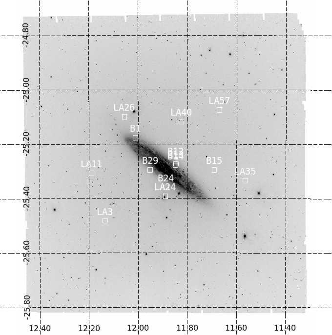
Figure 1: Full field of view observed with VST ($g$ band is shown, other bands are nearly identical). White squares indicate the 14 spectroscopic confirmed GCs from Beasley & Sharples (2000), labeled as in Table 2 (Col. 6) in that paper.

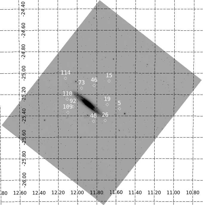
Figure 2: Full field of view observed with VISTA ($J$ band is shown, $K_{s}$ band is nearly identical). White diamonds indicate the 11 spectroscopic confirmed GCs from Olsen et al. (2004), labeled as in Table 3 (Col. 1) in that paper.

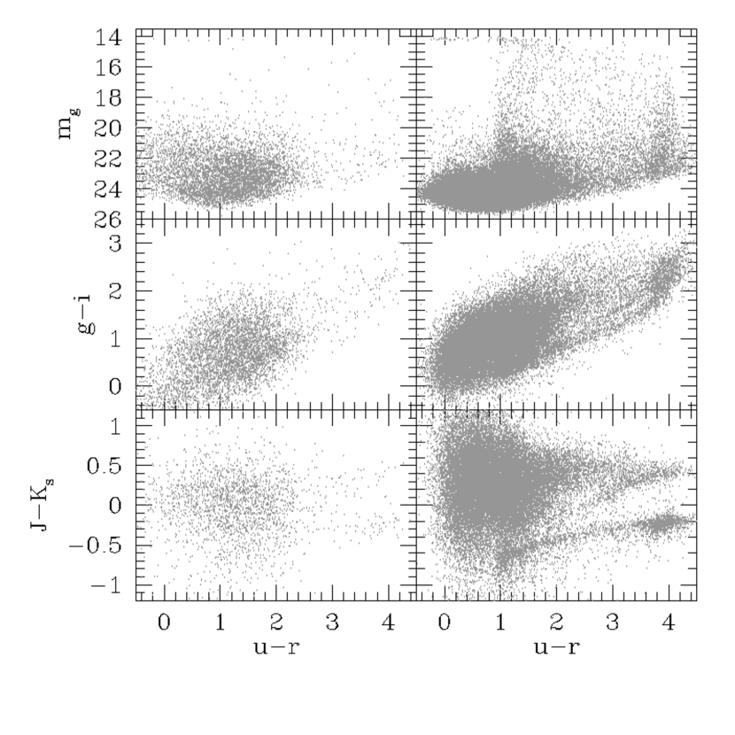
Figure 3: Color magnitude and color-color diagrams for the full matched catalog of sources detected. Left panels: Sources detected at galactocentric radii with moderate-to-high galaxy surface brightness background, $\mu_{g}\leq 23.6\leavevmode\nobreak\ mag/arcsec^{2}$, are shown. Right panels: Sources detected in regions with low galaxy background are shown.

3 Selection of GC candidates

To select GC candidates we applied the photometric, morphometric, and color selection criteria already used in Cantiello et al. (2017), with some differences explained below.

We started by applying color-color selections using all available pairs of colors. Figure 4 shows some examples of the color-color diagrams. In each panel, besides showing the full sample of matched sources in light gray, we highlight some stages of the GCs selection procedure adopted. For the purely optical color-color diagram (upper left panel), we plot the locus of simple stellar population models from the Teramo-SPoT group (Raimondo et al., 2005; Raimondo, 2009)

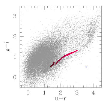
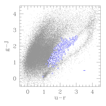
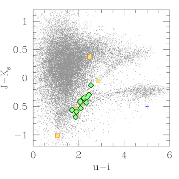
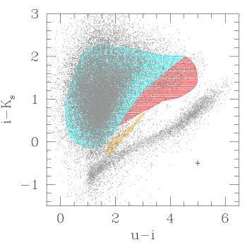
Figure 4: Selection of color-color diagrams used for selecting GC candidates. Gray dots show the full sample of matched sources. In each panel, in addition to the full sample, single elements of the GC selection process are highlighted. Upper left panel: SSP models for ages between 6 and 14 Gyrs and $[Fe/H]$ between $-$2.3 and $+$0.3 are plotted with solid lines in various shades of red (darker for more metal-poor; at fixed $[Fe/H]$ , older ages have redder colors). Upper right: Blue dots show the sample of $\sim 350$ GC candidates selected using color-color, photometric, and morphometric selection criteria described in text. The median error bars are indicated (lower right blue symbols), calculated as the sample median from GC candidates and shown in other panels as well. Lower left panel: Yellow squares and green diamonds indicate the location of Beasley & Sharples (2000) and Olsen et al. (2004) spectroscopically confirmed GCs. Lower right panel: We highlight the approximate MW stars sequence (gray), the area occupied by background galaxies (passive in red and blue star-forming galaxies in cyan; see also Appendix A), and the area identified by Muñoz et al. (2014) as the locus of GCs (orange).

For each pair of colors, we selected only the sources falling within the color-color area defined by confirmed GCs and SSP models as good GC candidates, extended by $\sim$20% on each side; i.e., no less than 0.2 mag for the colors spanning an interval lower than 1 mag, such as $r{-}i$. The choice of $\sim$20%, adopted after several tests, was motivated by the need for an area large enough to include the largest percentage of confirmed GCs, but not too wide to avoid exceedingly large contamination from obvious non-GCs sources. We adopted as lower age limit for SSP models $t=6$ Gyr, based on the comparison of the range of colors from confirmed GCs. Such limit might be rather low for the ages, generally $\ \raise-2.0pt\hbox{\hbox to0.0pt{\hbox{$\sim$}\hss}\raise 5.0pt\hbox{$>$}\ }10$ Gyr (e.g., Puzia et al., 2005), typical for old GCs. However, given the age-metallicity degeneracy for the optical colors (Worthey, 1994), younger SSP models with higher $[Fe/H]$ overlap with the sequence of older SSP models with lower $[Fe/H]$ . In any case, the main constraint to the color-color selections adopted here comes from empirical data. We used the SSP models as a countercheck, as they are confined to a very narrow region of the optical color-color planes, while empirical data are more scattered and also include the selection with near-IR bands.

To give an idea of the efficiency of the color-color selection adopted, we highlight that, starting from a sample of $\sim 1.200.000$ matched sources, the sample of color-color preselected GCs includes $\sim 1.500$ objects.

To further narrow down the sample of reliable GC candidates, we used other photometric and morphological properties of the sample, as described in Cantiello et al. (2017). We measured the magnitude concentration index (Peng et al., 2011), obtained as the difference between the magnitude measured at 6 pixel aperture diameter and at 12 pixel, $\Delta X_{6-12}\equiv mag_{X,6pix}-mag_{X,12pix}$ , where X is one of the optical $ugri$ bands and aperture corrected magnitudes are used. For point-like sources, after applying the aperture correction to the magnitudes at both radii, $\Delta X_{6-12}$ should be statistically consistent with zero. Hence, $\Delta X_{6-12}$ is an ideal tool to identify point-like sources, such as stars and extragalactic GCs in very distant galaxies as they appear unresolved. In the case of NGC 253, given the spatial resolution and FWHM of our dataset, GCs appear as slightly resolved extended sources and, consequently, their magnitude concentration index is larger than zero. By analyzing the sample of confirmed GCs, we find $\Delta X_{6-12}>0.1$ mag in all optical bands (with three exceptions discussed below), and a median of $\Delta X_{6-12}\sim 0.2$ mag. For the morphologic selection we did not use VISTA data as the pixel resolution is lower than for VST. Moreover, the $J$-band image is much more crowded than optical images; given the depth of the frame, stars in the field of NGC 253 are also detected (Greggio et al., 2014).

The upper left panel of Figure 5 shows the $g$-band magnitude concentration index, $\Delta g_{6-12}$, for the sample of color-color selected GC candidates. In the panel, where the confirmed GCs are also reported, the stellar sequence at $\Delta g_{6-12}\sim 0.0$ mag is easily recognized, as well as the positive, $\geq 0.1$ mag, values for all but three confirmed GCs. The three sources at $\Delta g_{6-12}\leq 0.075$ mag, which we adopted as threshold for reliable candidates, are the candidates with ID #109 and #114 from Olsen et al. (2004), and LA11 from Beasley & Sharples (2000). For the first two sources, we observe that the magnitude concentration index is consistent with zero in all optical bands and, similarly, the SExtractor and Ishape (see section 3.2) output parameters described below, are all consistent with the stellar nature of the two sources. Analyzing the two candidates in more detail, we also find that both have FWHM that is locally indistinguishable with all confirmed stellar sources (selected by colors and the other morpho-photometric criteria). The case of LA11 is described in more detail later in this section.

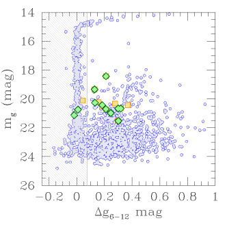
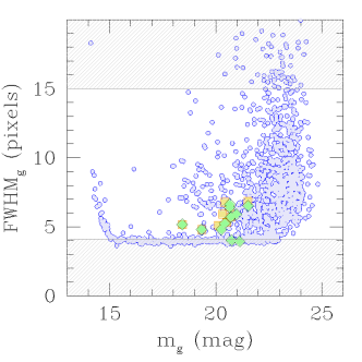
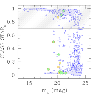
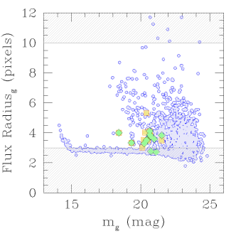
Figure 5: Upper left: $g$-band magnitude concentration index for the sample of color-selected GC candidates, shown in blue. As in Figure 4, yellow squares and green diamonds indicate the location of Beasley & Sharples (2000) and Olsen et al. (2004) spectroscopic confirmed GCs, respectively. The gray shaded area defines the region in which sources are rejected as reliable GC candidates. Upper right: $g$-band FWHM from SExtractor vs. magnitude. Symbols are as upper left panel. Lower left: As upper right, but SExtractor CLASS_STAR parameter is plotted instead of FWHM. Lower right: As upper right, but SExtractor Flux Radius (i.e., half-light radius) parameter is plotted instead of FWHM. The saturation that is manifested as the rightward tail at bright magnitudes in the upper left panel, similar to the tail that points upward in the upper right and lower right panels, appears at a magnitude brighter than the brightest GCs (e.g., $m_{g}<15.5$ mag; see also Table 2), and therefore does not affect our GC candidate selection process.

As additional selection criteria, for the sole optical bands, we used a selection of SExtractor output parameters (i.e., FWHM, CLASS_STAR, minor-to-major axis ratio $b/a$, and flux radius; see definitions in Table 2), the limits of the GCLF, and a maximum photometric error. The SExtractor selection criteria were derived by comparison with the same parameter for confirmed GCs; for the minimum axis ratio, $b/a$, we conservatively assumed $b/a\geq$0.67, which is comparable to the observed minimum for MW and Magellanic Clouds GC systems (van den Bergh & Morbey, 1984; Harris, 1996; Cantiello et al., 2009). The FWHM, CLASS_STAR, and flux radius selections are also shown in Figure 5.

There is some level of degeneracy for some of the adopted morphometric quantities. Our intention, in adopting such large set of parameters, is to exclude anomalous or peculiar sources that might be more efficiently detected with one parameter rather than others, hence minimizing any contamination from non-GC sources.

The bright and faint magnitude cuts were derived from the GCLF as follows. We adopted the RGB-tip distance modulus given in Table 1 and then we used the results from Villegas et al. (2010) for the GCLF turnover magnitude (TOM or $M_{TOM}$, hereafter) and for the GCLF dispersion, $\sigma_{GCLF}$. In particular, we adopted $M^{g}_{TOM}=-7.4$ mag and estimated $\sigma_{GCLF}=1.1$ mag (assuming a total magnitude of NGC 253 of $M_{Z}\sim-22$ mag). Finally, we adopted as magnitude cuts $\pm 3\sigma_{GCLF}$ brighter and fainter than the TOM. For sake of simplicity, the TOM in $u$, $r,$ and $i$ bands, were derived from the $M^{g}_{TOM}$ band reported above, and from the median $u{-}g$, $g{-}r,$ and $g{-}i$ of known GCs in the sample, i.e., $\sim 1.4,\leavevmode\nobreak\ 0.6,$ and 0.8 mag, respectively. Furthermore, to be most inclusive as possible, the magnitude cuts were rounded off to the closest more conservative semi-entire magnitude (e.g., we adopted $m^{bright}=16$ for the $r$ band rather than 16.2 mag, and $m^{faint}=23$ rather than 22.8 mag).

Table 2: Photometric and morphometric selection criteria adopted

Quantity	Passband	Range adopted
		for selection
$\Delta X_{6-12}$ (mag)	All	$\geq 0.075$
CLASS_STAR	$u$	$\leq 0.8$
CLASS_STAR	$g$	$\leq 0.7$
CLASS_STAR	$r$	$\leq 0.95$
CLASS_STAR	$i$	$\leq 0.95$
PSF FWHM (pixels)	$u$	$\geq 4.5$
PSF FWHM (pixels)	$g$	$\geq 4.1$ & $<15$
PSF FWHM (pixels)	$r$	$\geq 4.25$ & $<15$
PSF FWHM (pixels)	$i$	$\geq 3.9$ & $<15$
Flux Radius (pixels)	$u$	$\geq 3.2$ & $<10$
Flux Radius (pixels)	$g$	$\geq 3$ & $<10$
Flux Radius (pixels)	$r$	$\geq 3$ & $<10$
Flux Radius (pixels)	$i$	$\geq 2.5$ & $<15$
Axis Ratio b/a	All	$\geq 0.67$
$\Delta$ mag	All	$\leq 0.25$
$m^{bright}$-$m^{faint}$ (mag)	$u$	18-25
$m^{bright}$-$m^{faint}$ (mag)	$r$	16.5-23.5
$m^{bright}$-$m^{faint}$ (mag)	$g$	16-23
$m^{bright}$-$m^{faint}$ (mag)	$i$	16-23

All the morpho- and photometric selection criteria adopted are summarized in Table 2. The final sample of selected GC candidates, passing through all adopted selections, contained $\sim 350$ sources.

In Figure 6 we show some of the color-color diagrams already shown in Figure 4, but this time plotting only the $\sim 350$ GCs candidates selected using the photometric, morphometric, and color selection criteria described above. Overplotted in green and yellow symbols are spectroscopically confirmed GCs. In addition, a color magnitude diagram (upper right panel) is reported.

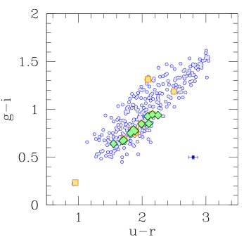
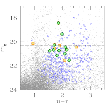
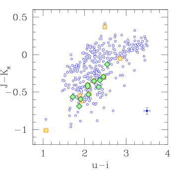
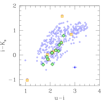
Figure 6: Color-color (upper left and lower panels) and color-magnitude (upper right) diagrams of the $\sim 350$ selected GC candidates (blue circles) and the spectroscopically confirmed GCs. Yellow squares and green diamonds indicate the Beasley & Sharples (2000) and Olsen et al. (2004) samples, respectively. For the color-magnitude diagram, the full sample of matched sources (gray dots) and the position of the turnover magnitude (long-dashed horizontal black line) are also shown.

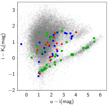
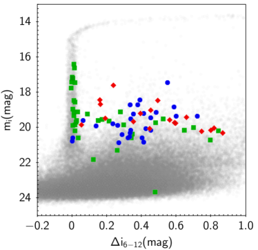
Figure 7: Color-color ($uiK_{s}$, left) and $i$- band concentration index ($\Delta i_{6-12}$, right) diagrams for the full matched catalog (gray symbols) and the photometric GC candidates from the literature. Red diamonds, blue circles, and green squares indicate Liller & Alcaino (1983), Blecha (1986), and Beasley & Sharples (2000, Table 6) GC candidates, respectively.

3.1 Comparison with spectroscopic and photometric GC samples

Our sample of $\sim 350$ color-color, morpho- and photometric selected GC candidates does not contain some of the spectroscopically confirmed sources by either Beasley & Sharples (2000) or Olsen et al. (2004). We already anticipated the cases of 2 out of 11 GCs from Olsen et al. (2004, IDs #109 and #114 from their Table 3), which are consistent with being foreground stars in all bands, including $J$ and $K_{s}$, as they are coherently consistent with stellar morpho-photometric parameters. The two objects have line-of-sight velocity of $177\pm 5\leavevmode\nobreak\ km/s$ and $192\pm 17\leavevmode\nobreak\ km/s$, which are relatively high and explain their classification as GCs in NGC 253, which has $cz=243\pm 2$ km/s. Nevertheless, the photometric properties of the couple indicate they are likely high-velocity MW stars (e.g., Xue et al., 2008). The remaining 9 sources from Olsen et al. are correctly selected as GCs in our final sample.

As for the sample of confirmed GCs by Beasley & Sharples (2000), the clusters with IDs LA11, LA24, B1, B13, B14, and B29 from their Table 2 (we adopted the alternative IDs given by the authors), are not selected. Because LA24 is very close to a bright star ($m_{V}<9$ mag), this GC is undetected in some passbands, while B1 is undetected in the $K_{s}$ band because it is faint.

The other missing four candidates are excluded from our sample because of their colors (LA11 also for its concentration index, see Figure 5). The rejected candidates are shown in the RGB thumbnail of Figure 9. The candidate LA11, in addition to the non-GC colors, shows the presence of obvious features in all the imaging data from VST; for B29, its red colors are consistent with a background early-type galaxy; this possibility is also supported by its elongation, which exceeds our adopted $b/a$ limit of 0.67, with both the SExtractor and Ishape analyses. Hence, for both the latter objects, our analysis rather supports the non-GC nature of the two sources.

Sources B13 and B14 appear deeply enshrouded in the dust of the galaxy. Hence, because of host-galaxy extinction, the colors of the sources were off the color-color areas we adopted.

All such missed sources are in any case included in the final table of GC candidates, properly commented in our classification scheme.

As for the comparison with previous photometric catalogs of GCs, in Figure 7 we plot some properties of our full catalog of matched sources with the samples of photometric candidates from Liller & Alcaino (1983), Blecha (1986), and Beasley & Sharples (2000). In addition to the spectroscopic sample used here, the latter authors presented a sample of $\sim 90$ photometrically selected GCs. The figure highlights that a substantial number of selected candidates are indeed stars or background galaxies, both because of their colors or the concentration index, or both. The improved efficiency of the analysis presented here is due to a combination of the larger inspected area, which is a factor of $\sim$3 to $\sim 10$ with respect to previous studies, the better seeing conditions, from 10% better to 300%, and the much wider wavelength coverage; other studies are based on only $B$ or $B$ and $V$ photometry.

3.2 Globular cluster sizes

At the distance of NGC 253, and with the seeing conditions of our observational dataset, the half-light radii $R_{h}$ of GCs can be derived. Size measurements can be very challenging, especially with ground-based imaging data. In spite of this, angular sizes and intrinsic shapes have been obtained for a large sample of slightly resolved star clusters in different environments and with various ground- and space-based telescopes (e.g., Larsen, 1999; Larsen & Brodie, 2003; Jordán, 2004; Cantiello et al., 2007; Caso et al., 2013; Puzia et al., 2014; Cantiello et al., 2015).

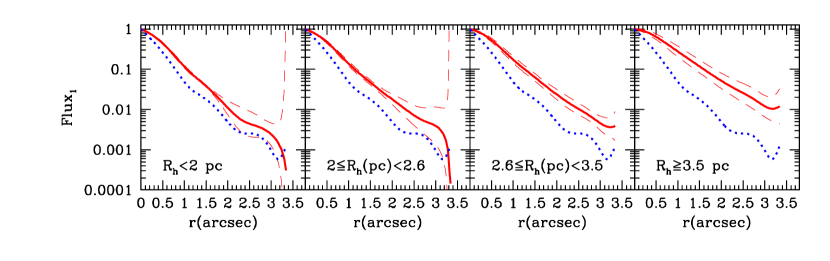
Figure 8: Radial flux profiles of GCs in $g$ band. The various panels show the average flux profile (solid red lines, normalized to one at center) for GC candidates with measured $R_{h}$ within the labeled interval. Thin dashed lines show the standard deviation of the mean for the average profile; blue dotted line indicates the PSF profile.

To estimate the intrinsic size of a source exceeding some instrumental-dependent size limit, specific tools have been designed and implemented to analyze the light profiles of sources with intrinsic sizes comparable or slightly smaller than the instrumental point spread function (PSF). We adopted Ishape to obtain structural parameters (in particular $R_{h}$ and the minor-to-major axis ratio $b/a$) of candidate GCs. Ishape is optimized for modeling the light distribution for marginally resolved sources down to 1/10 of the FWHM of the PSF (Larsen, 1999; Larsen & Richtler, 2000). In such context, the VST dataset of NGC 253 is very attractive. At the adopted distance modulus (corresponding to $\sim 3.47$ Mpc), and given the FWHM of the images (Table 1), Ishape can be used to determine the physical extent of objects with $R_{h}\geq 1.3$ pc. For reference, excluding highly extincted GCs, with $E(B-V)\geq 0.5$, the MW hosts two GCs with $R_{h}\ \raise-2.0pt\hbox{\hbox to0.0pt{\hbox{$\sim$}\hss}\raise 5.0pt\hbox{$<$}\ }1.2$ pc and five with $R_{h}\leq 1.5$ pc (Harris, 1996). The median is $R_{h}=3.22$ pc. Since the measurement of source sizes below the FWHM is particularly demanding in terms of signal-to-noise ratio and image quality, we limited the analysis of GC radii to $gri$ band data. Using Ishape, we fitted all sources with a King profile with concentration index c=15 (Larsen, 1999; Larsen & Richtler, 2000). The final $R_{h}$ and $b/a$ values are derived from the weighted average of the three bands.

Figure 8 shows the $g$-band radial flux profile of our bona fide GC candidates (see next section; flux is normalized to peak one), compared with the radial profile of the PSF in the same band. In this panel we plot the average profile of GCs with estimated effective radii within the labeled $R_{h}$ intervals. The width of the $R_{h}$ intervals is chosen to contain similar numbers of GC candidates ($\sim 20$) per $R_{h}$ bin. The figure shows the significant differences between PSF (i.e., stellar) and GCs light profiles even for the most compact candidates, reported in the left panel. Hence, unlike typical studies of extragalactic GCs (e.g., Durrell et al., 2014), MW stars represent a minor source of contamination in our GC catalog because of the combined effect of galaxy distance, GC physical size, and good image quality.

Finally, we specifically run Ishape on the two sources from Olsen et al. (2004) that we identified as stars (IDs #109 and #114, mentioned in previous section). The results confirm the single star origin of the two sources, as their $R_{h}$ are consistent with zero in all three inspected bands, and the $\chi^{2}$ for the fit to an extended source does not improve with respect to the $\chi^{2}$ obtained modeling a compact, stellar source.

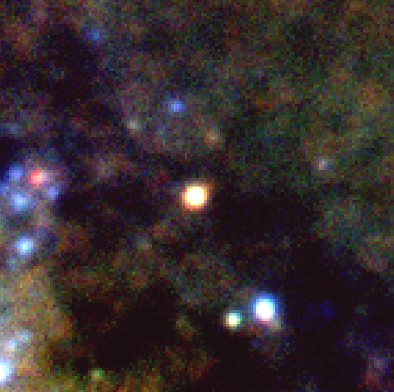
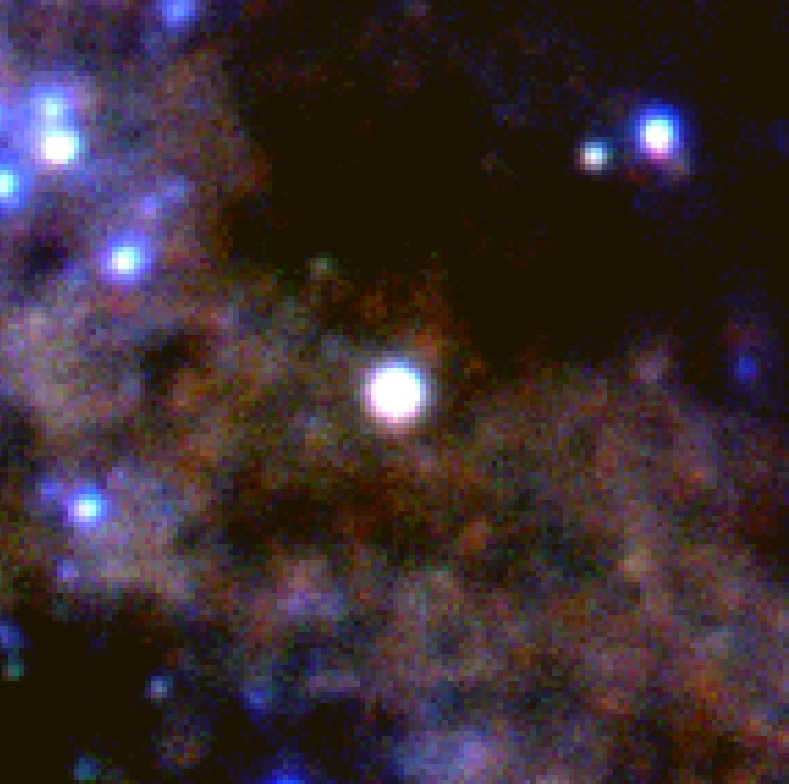
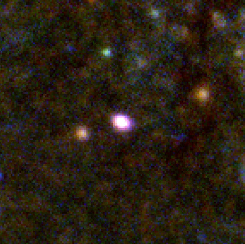
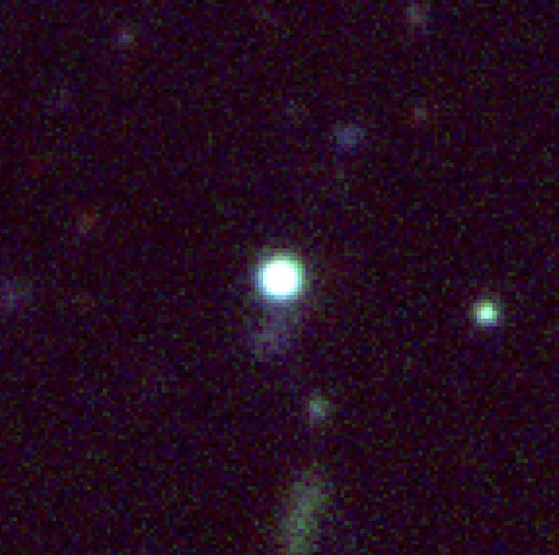
Figure 9: RGB thumbnails from VST data of star cluster candidates from Beasley & Sharples (2000) that did not pass our selection criteria for GC candidates. Starting from left: B13 and B14 (close to galaxy dusty regions), and B29 and LA11 (likely background galaxies). Thumbnails are 15$\arcsec$ on each side.

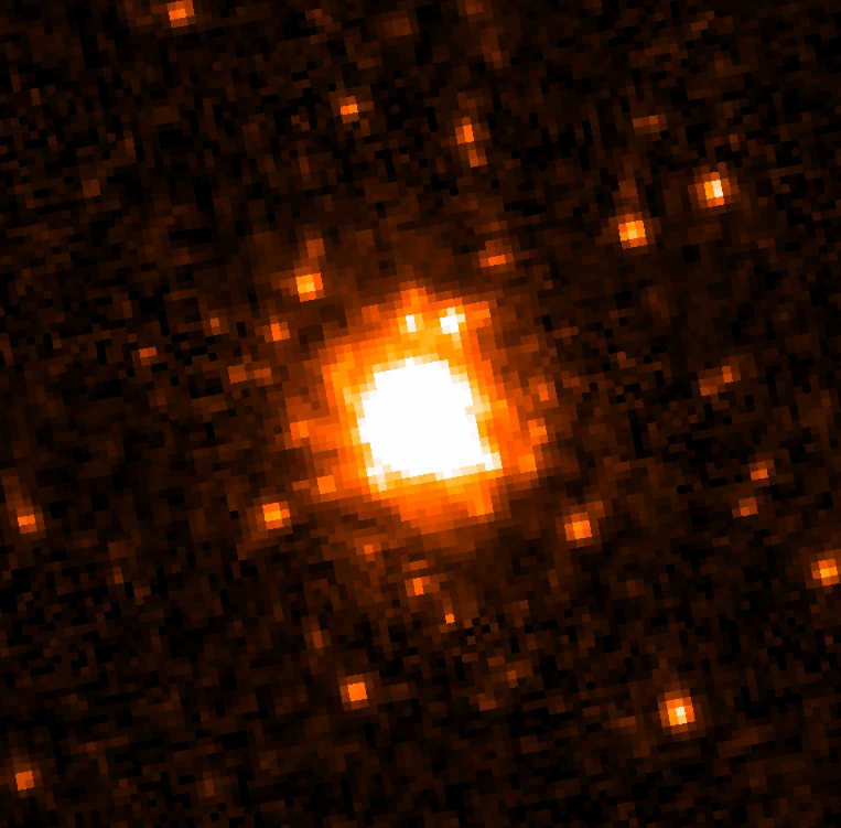
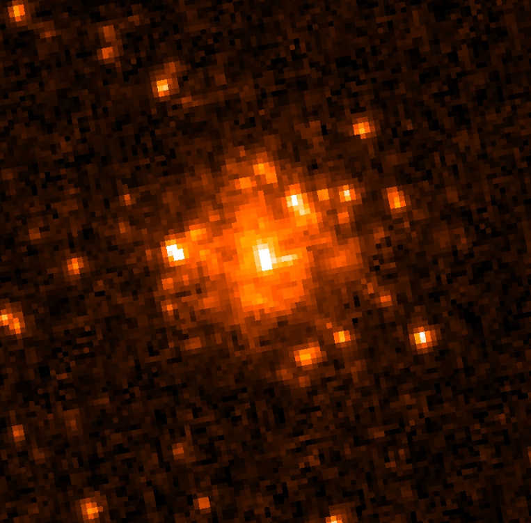
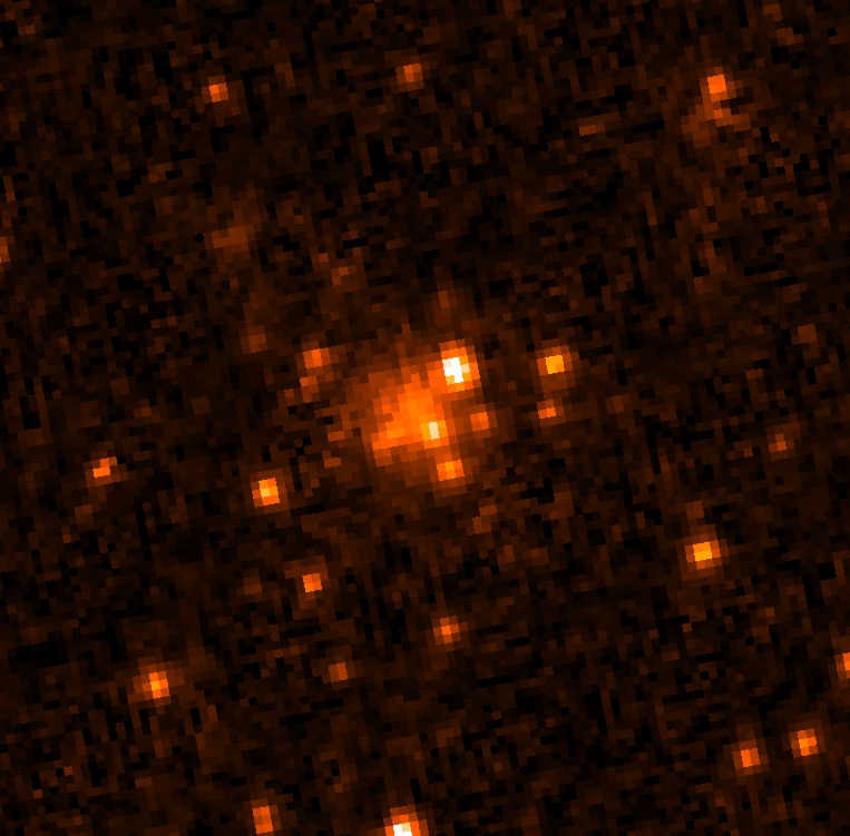
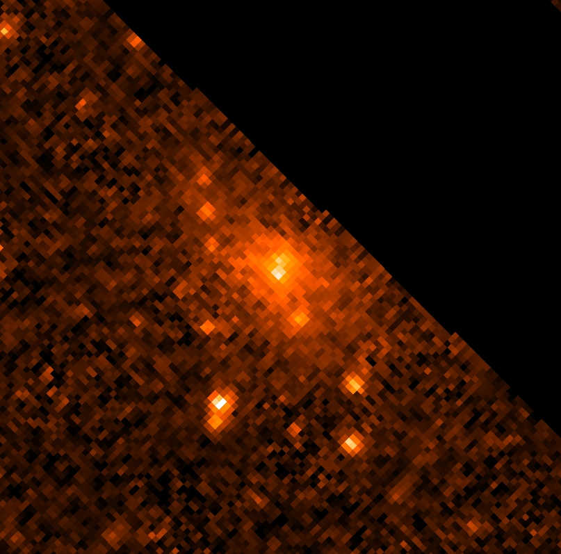
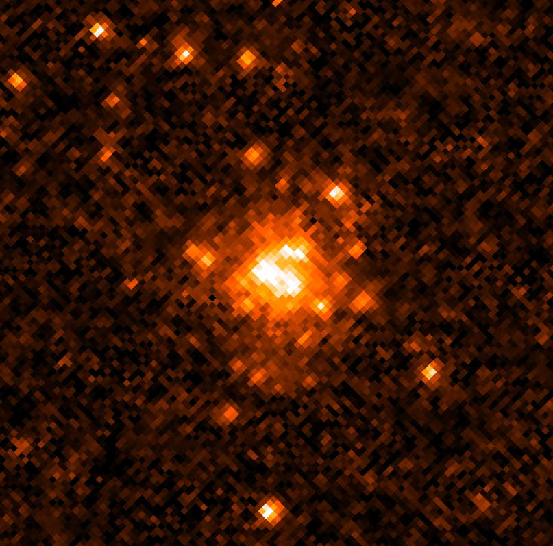
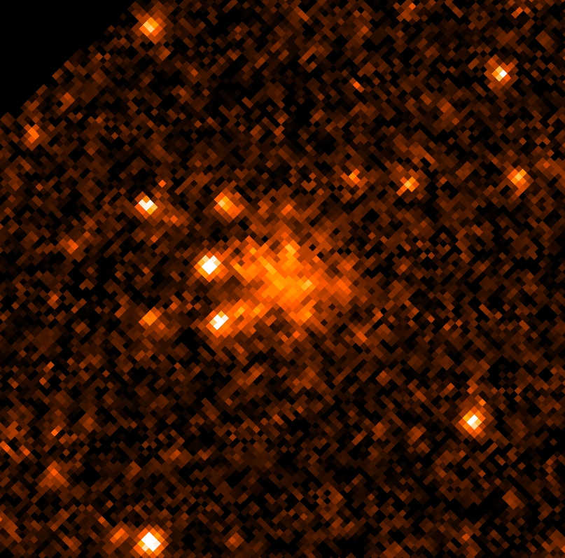
(a) From left to right: Cluster candidates number #99, #109, #111, #124, #128 and #141 in Table LABEL:tab_final.

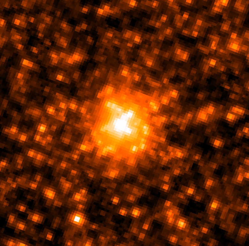
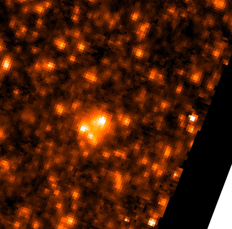
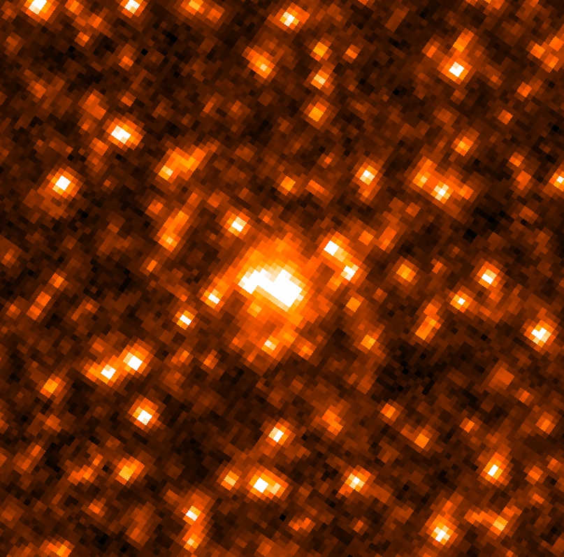
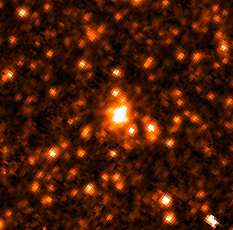
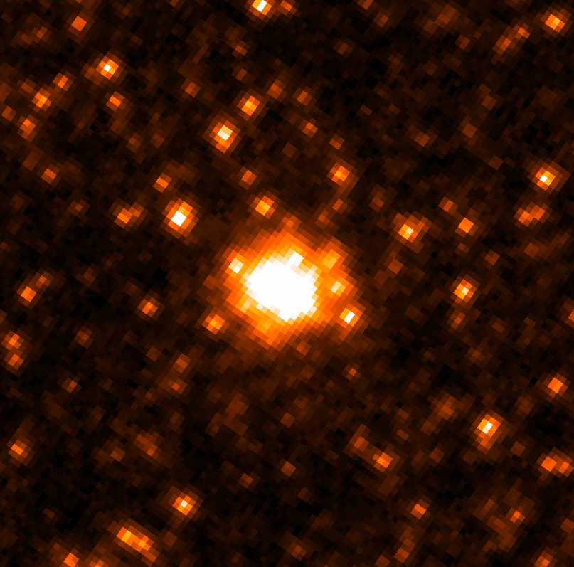
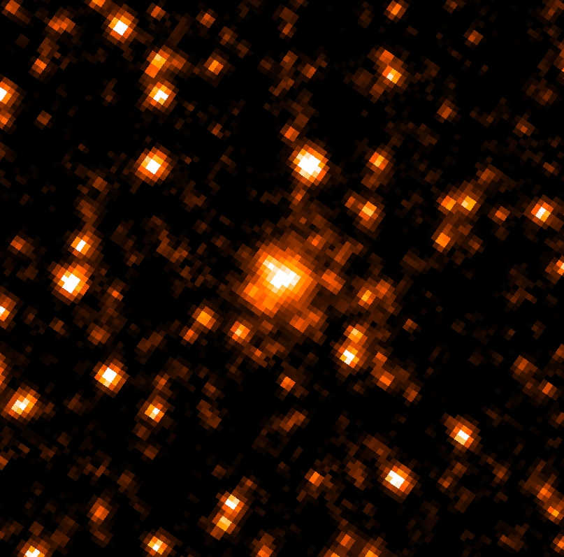
(b) From left to right: Cluster candidates number #178, #186, #200, #204, #205 and #207, in Table LABEL:tab_final.

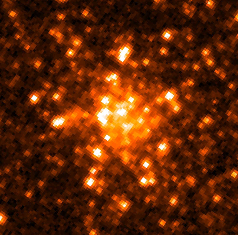
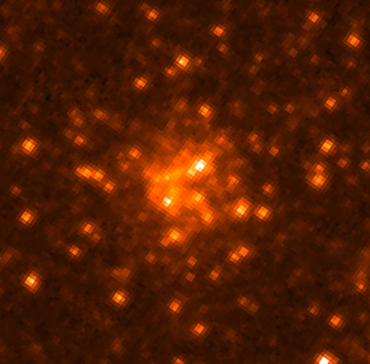
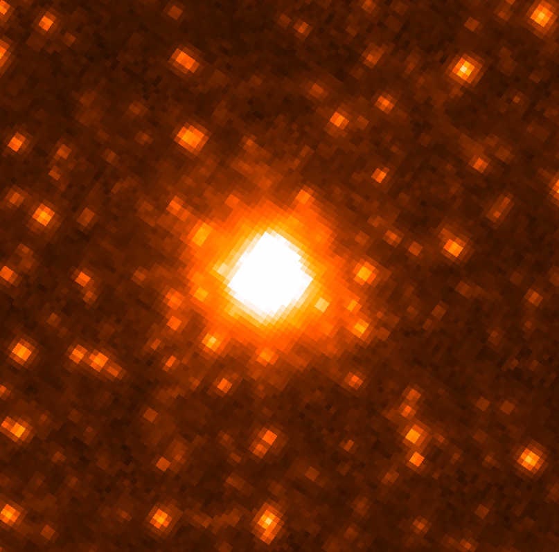
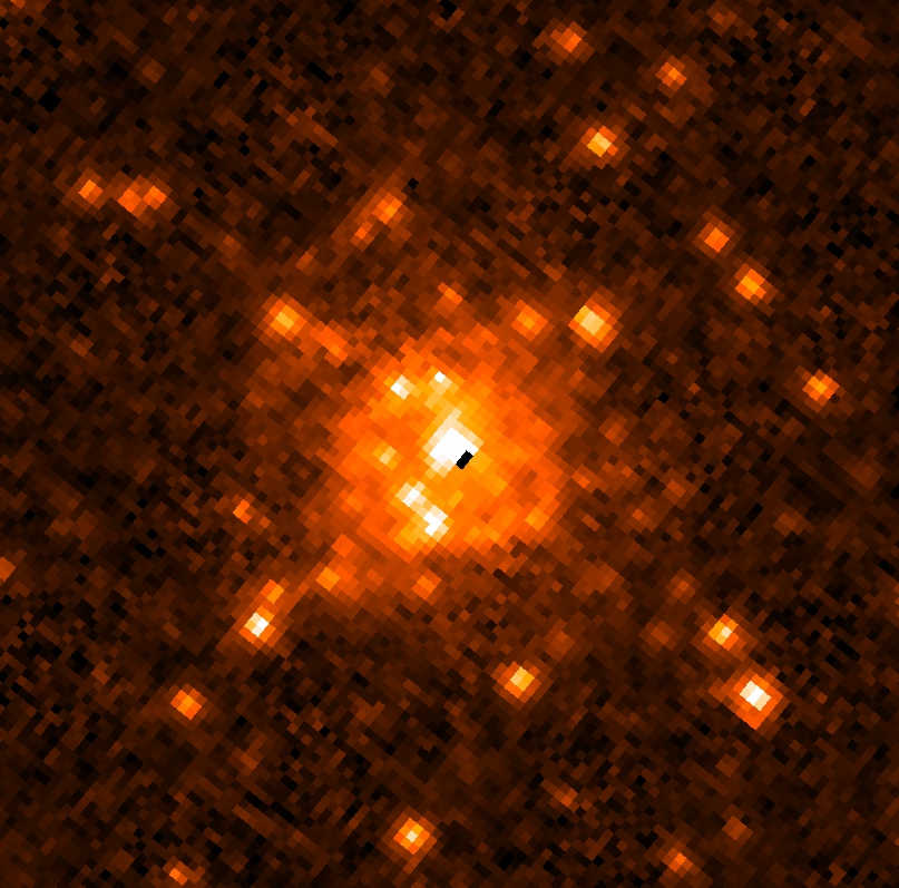
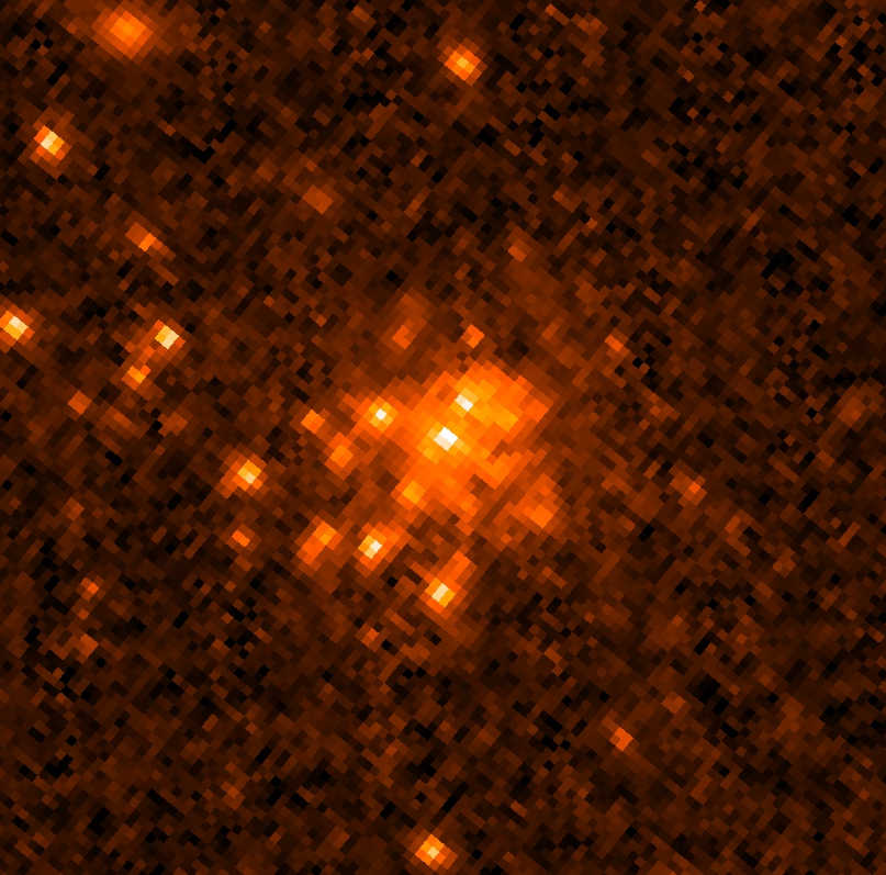
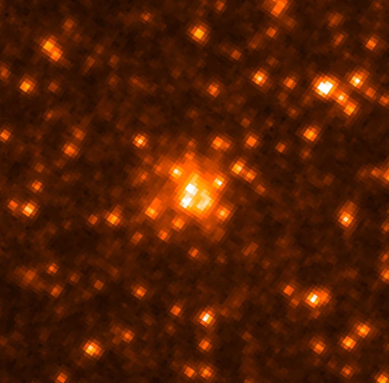
(c) From left to right: Cluster candidates number #209, #210, #211, #218, #227 and #325 in Table LABEL:tab_final.

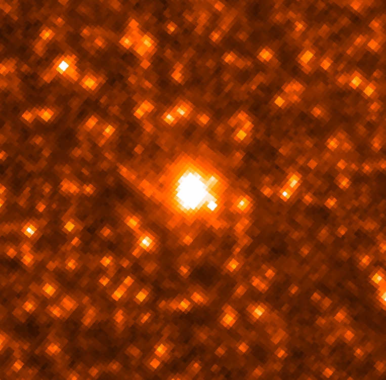
(d) From left to right: Cluster candidates number #333, #334, #335 and #336 in Table LABEL:tab_final.

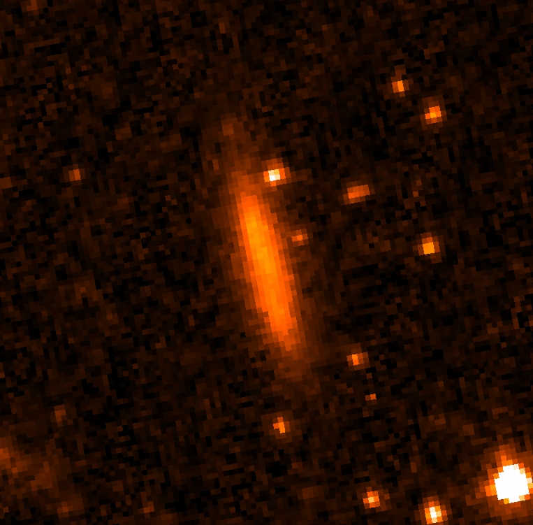
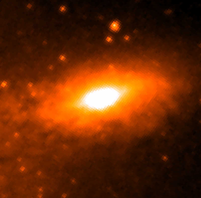
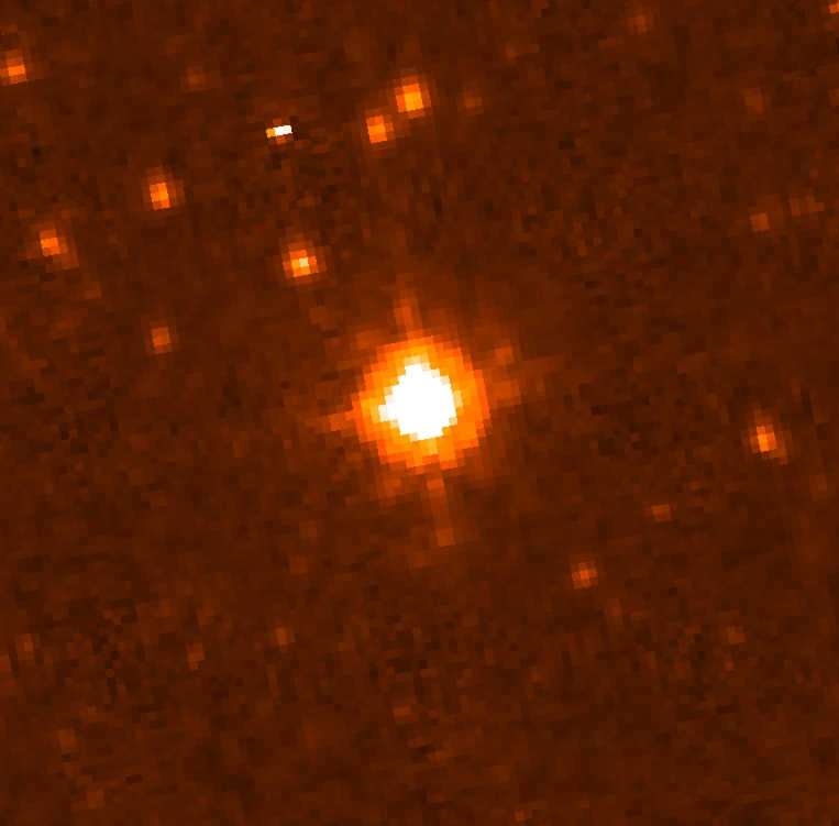
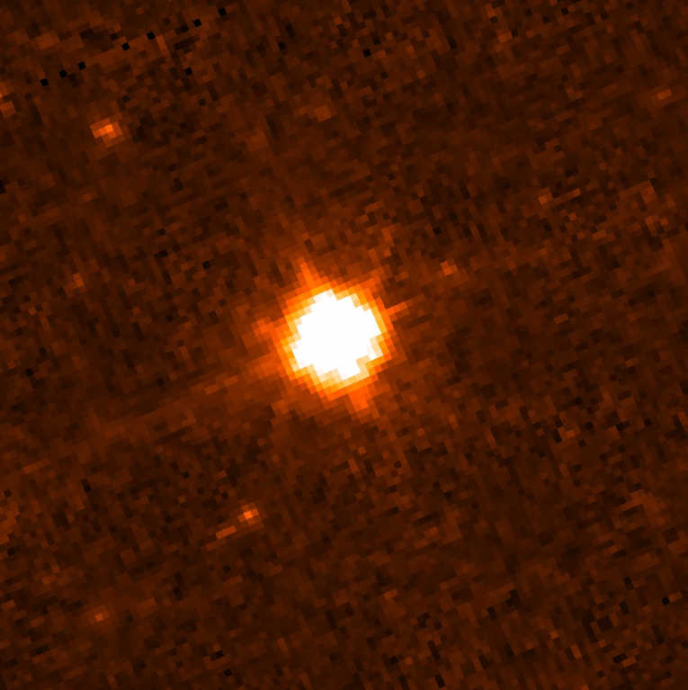
(e) From left to right: Sources #107 and #212 in Table LABEL:tab_final (confirmed background galaxies), and two of the sources identified as stars in our selection procedure.

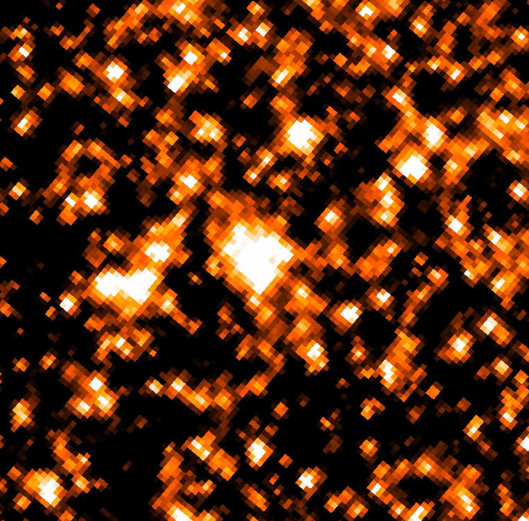
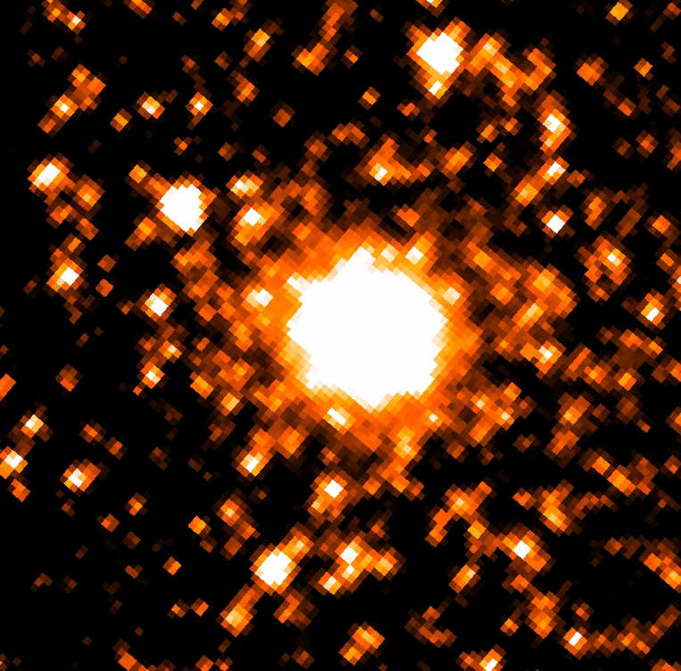
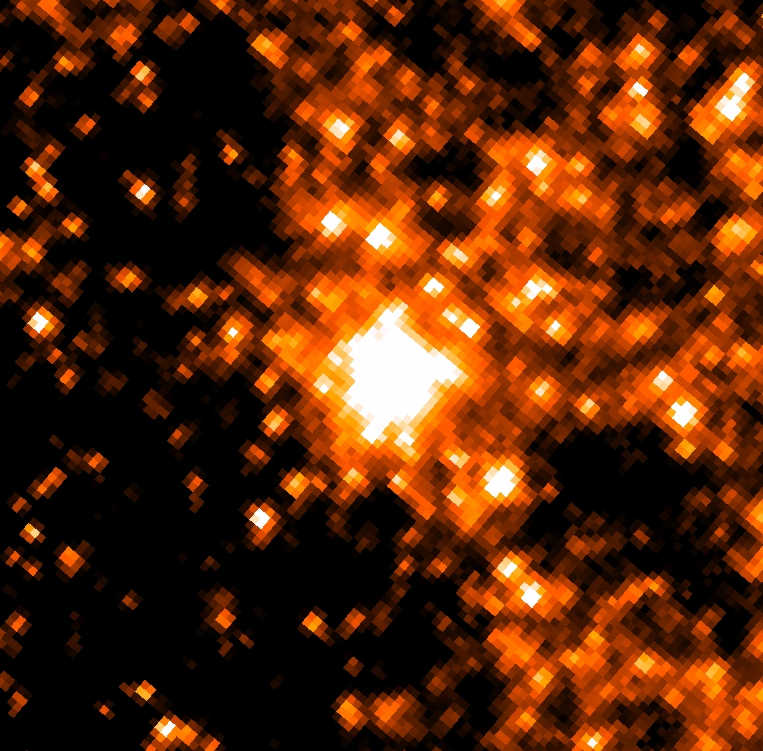
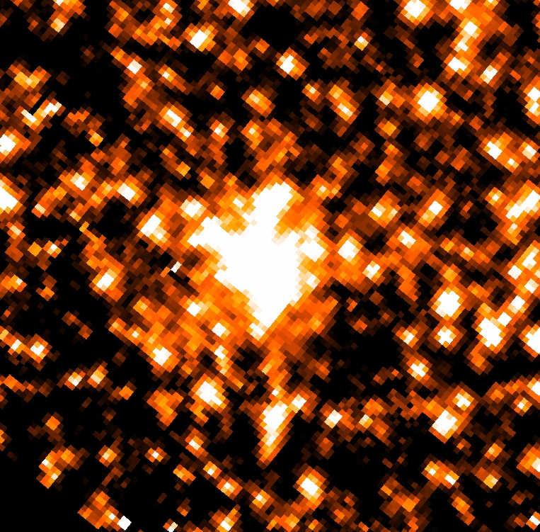
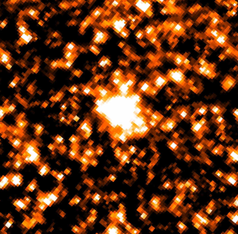
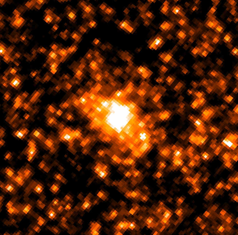
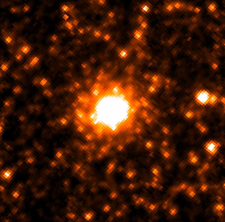
(f) From left to right: Sources #326, #327, #328, #329,#330, #331 and #332 in Table LABEL:tab_final visually identified as GCs, and located within the dust disk of NGC 253.

Figure 10: Upper four rows (a-d): Hubble Space Telescope ACS cutouts of the sources selected as GCs candidates and falling in the GHOSTS survey footprints (F814W-band imaging data are shown). Given the mottled appearance, we consider all sources as star clusters in the galaxy. For reference, the panels in row (e) show the other two selected sources in the GHOSTS footprints, which are obvious background galaxies, and two stellar sources. The sources in the row ($f$) are the visually identified GC candidates (see text).

4 Final catalog and discussion

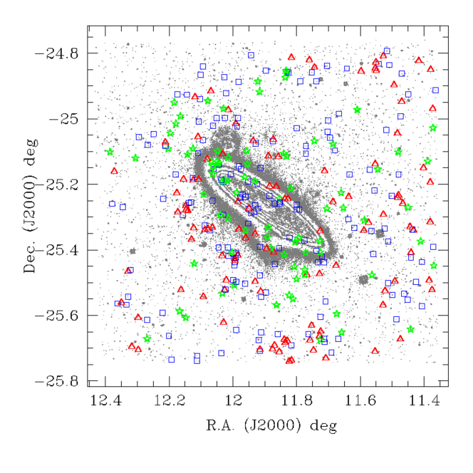
Figure 11: GC candidates overlaid to the $g$-band contour plot of NGC 253. Green five-pointed stars, blue squares, and red triangles show the candidates flagged as Best, Uncertain, and No in Table LABEL:tab_final, respectively. The plotted contours show the $\mu_{g}=$23.6, 23.0, 22.4, 21.8, 21.2, 20.6 $mag/arcsec^{2}$ surface brightness levels, respectively.

4.1 The catalog

Taking advantage of the ACS Hubble Space Telescope observations of NGC 253 from the GHOSTS survey (the GHOSTS acronym stands for: Galaxy, haloes, outer disks, substructures, thick disks, star clusters Radburn-Smith et al., 2011), as a countercheck of our selection, we visually inspected the GHOSTS fields containing our GC candidates. Thanks to the exceptional resolution of ACS, star clusters at the distance of NGC 253 appear as obviously mottled and extended sources with respect to the otherwise smooth background galaxies or point-like stellar sources. With the exception of two obvious background disk galaxies, all of the sources selected as described in the previous section, and falling in the ACS GHOSTS footprints, appear as star clusters. Figure 10 shows the thumbnails of the 18 selected GC candidates that also have HST data (panels from $(a)$ to $(d)$). In the figure we also show the two background galaxies that passed our GC selections and, for sake of comparison, two sources identified as stars in our selection procedures (panel ($e$)).

Furthermore, some visually obvious GCs in the GHOSTS footprints, which were not selected by our procedure, were added by hand in our final sample, after visual inspection of GHOSTS images. Such objects, seven in all (Figure 10, panel ($f$)), although detected and classified as extended in all cases, were rejected from the final sample as their colors did not fit in the color-color sequences adopted because of dust contamination. Although based on their appearance the candidates are certain stellar clusters, in our final Table LABEL:tab_final they are flagged as Uncertain because of their color, and excluded from the color and magnitude distributions analysis discussed below.

Moreover, still based on comparison with GHOSTS data, in spite of the rich set of selection criteria adopted, including the $uiK_{s}$ color-color diagram that proved to be very effective for sorting GCs out of other sources in Virgo (Muñoz et al., 2014), the matching with HST imaging data shows the presence of background contamination in the final list of GC candidates. Thus, for a final characterization of the GCs selected and to further clean the sample, we visually inspected each one of the $\sim 350$ GC candidates.

From the visual inspection we found that a substantial portion of selected candidates are obvious galaxies for various motivations: more or less obvious features visible in one or more bands (tidal features, spiral arms), high elongation coupled with closeness to a group of background galaxies, bright and elongated structures with changing position angle at different radii, etc.

Table LABEL:tab_final lists the final sample of objects with coordinates (Cols. 2-3); $ugriJK_{s}$ magnitudes and errors (Cols. 4-9); half-light radius and axis ratio from Ishape (Cols. 10-11); existing identifications from the literature (Col. 12); presence in GHOSTS footprints, spectroscopic samples, or previous identifications in the photometric samples by Liller & Alcaino (1983) or Blecha (1986) (Col. 13); and comments from visual inspection (Col. 14). In the table we also provide a further flag, Class (Col. 15), which defines the objects classified as bona fide GC candidates in our list, the candidates considered uncertain for some reason (large number of close background galaxies, high elongation, weird residuals from Ishape, blending features, border-line axis ratio, etc.), and sources that are obvious galaxies (no flag), which passed morpho-photometric selection criteria, but were rejected upon visual inspection.

The catalog contains a total of 82 best GC candidates, 155 uncertain candidates, and 110 sources which, although passed all our GC selection criteria, are clearly background galaxies.

The spatial distribution of the full sample is shown in Figure 11, overlaid to the $g$-band VST contours plot.

We must note that our selection technique, based also on aperture photometry, leaves unanswered the question about the detection efficiency and contamination rate as a function of galactocentric radius. Although the majority of the globular cluster candidates are found in the uncrowded outskirts of the galaxy, a significant number are projected against or near the bright, crowded galaxy disk.

As is also recognizable in Figure 3, sources detected in regions of high galaxy background suffer from a larger photometric scatter because of the galaxy contamination and the presence of dust.

However, of the $\sim 20$ bona fide GCs candidates located in galaxy regions with $\mu_{g}\leq 23.6\leavevmode\nobreak\ mag/arcsec^{2}$, only four are new selections, the remaining are all either spectroscopically confirmed GCs or star clusters selected on HST/GHOSTS data, and three are also photometric selections from Beasley & Sharples (2000, Table 6 data).

4.2 Spatial distribution and luminosity function

The optical LF of the bona fide sample and the combination of the bona fide and uncertain samples are shown in Figure 12 (left panels). In the panels of the figure the $M_{TOM}$ adopted, properly shifted to the galaxy distance, is also reported. The diagrams lack the typical symmetry around the peak of the Gaussian GCLF, which is surprising given that the bright side of the LF appears underpopulated. By inspecting the full sample of sources brighter than $m_{g}\sim 20$, we found that even after adopting reasonably broader selection criteria the list of bright candidates does not increase. Hence, we do not have an explanation for missing bright end of the GCLF.

Taking only the sample of spectroscopically confirmed GCs does not improve the appearance of the GCLF because of the small size of the sample of 21 candidates and because 7 of the candidates are brighter than the $M_{TOM}$, and 14 are fainter than that, with the faintest candidate at $m_{g}\sim 21.5$ mag, i.e., at $\sim 1\sigma_{GCLF}$ the level of the faint side GCLF. If we also add the GCs identified over the HST/GHOSTS area, the cumulative sample of HST and spectroscopic candidates has $\sim 10$ GCs that are brighter than the $M_{TOM}$ and 41 fainter than the $M_{TOM}$. Hence, whether only the spectroscopic candidates or both spectroscopic and GHOSTS candidates are considered, again the GCLF is highly undersampled toward bright GCs.

The incompleteness is in part due to the photometric incompleteness, which is caused by the different depth and image quality of the imaging data adopted. However, photometric incompleteness should only be an issue at the faint end of the GCLF.

An alternative explanation for the asymmetric GCLF would come from overestimated low luminosity end of GCLF that would, even in the case of best candidates, have to be heavily contaminated. We believe this is not the case and thus reject this (potential) explanation because we have verified our selection criteria through a comparison with HST GHOSTS images and with a spectroscopically confirmed sample of GCs. Furthermore, if the low luminosity end were heavily contaminated, the GC sample size in NGC 253 would be too small, resulting in too small $S_{N}$, as we discuss further in Section 4.3.

A further correction to the GCLF might come from the fact that, in addition to photometric incompleteness, our sample is also incomplete at large and small galactocentric radii. The largest projected galactocentric distance of a GC candidate in the bona fide sample is $r_{gal}\sim 35\arcmin$, or $\sim 35.5$ kpc. A fraction of $\sim 7\%$ (11 out of 158) MW GCs are located at galactocentric distance larger than $\sim$35.5 kpc. Hence, it is reasonable to expect that a similar fraction of GCs in NGC 253 lies beyond the common area of the VST and VISTA pointings.

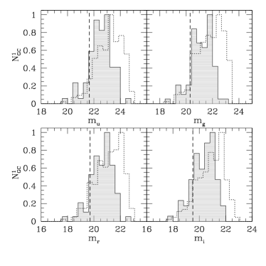
Figure 12: Left: Optical LFs of the bona fide sample GCs (gray shaded histogram) and of the bona fide+uncertain samples (dotted line). The adopted TOM in each band is shown with a vertical dashed line. Right: LFs of bona fide GCs, shown in logarithmic scale. The long-dashed line shows the power-law fit to the data. The exponent of the fit is reported each panel (see text).

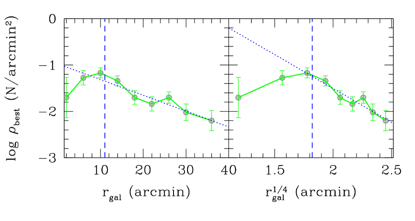
Figure 13: Radial density profile of the best GCs sample. Left and right panels show the linear and $r^{1/4}$-law profile, respectively. Linear fits to data are shown with blue dotted line. The vertical dashed line indicates the semimajor axis where the dusty disk begins.

For the central dusty regions, as aforementioned, we partially recovered some of the GCs by complementing our data with the ACS GCs from GHOSTS. Nevertheless, such detections, mostly based on visual inspection, do not necessarily allow the recovery of the entire population of central GCs in the galaxy. As a check, we inspected the azimuthal average of the GCs radial density profile, reported in Figure 13. The diagram shows the linear and $r^{1/4}$ fits to the density profile, which is derived without the data for the innermost two annuli, severely affected by dust and incompleteness. In both panels we observe a drop of the density profile in the very central regions, otherwise the radial (logarithmic) density profile nicely follows the fitted density profiles. The $r^{1/4}$-law profile, together with the increasing or flattening of the GC density profiles at small galactocentric radii, are well-known observational properties of GC systems (Dirsch et al., 2005; Goudfrooij et al., 2007; Cantiello et al., 2015). Consequently, it is reasonable to assume that the drop in $\log\rho(r_{gal}),$ seen in the left panels of Figure 12, is due to poor GCs detection in such central dusty regions. Even though the central area dominated by dust is relatively small, $\sim 80$ square arcmin, the fraction of GCs there could be significative. To obtain an approximate estimate of the number of GCs in the central area, we adopted the radial density profiles shown in Figure 13, assuming as lower limit to the GCs density the value of $\rho(r_{gal})$ at $r_{gal}\sim 11\arcmin$, i.e., the galactocentric radius where the dusty disk begins. Adopting the linear or $r^{1/4}$-law fits, the fitted GC density at $r_{gal}\sim 11\arcmin$ goes from $\sim 0.045$ GCs/$arcmin^{2}$, to $\sim 0.057$ GCs/$arcmin^{2}$. Hence, the estimated number of GCs in the central area is $N_{GC}^{center}\sim 5$.

In a study of RGB-tip field star population based on $V$ and $I$ Magellan/IMACS data, Bailin et al. (2011) found evidence for a large shelf-like feature near the southeast side of NGC 253 (also confirmed by Greggio et al., 2014, from resolved star analyses of the VISTA imaging data used in this work). Using GHOSTS data in two fields - one on and one off the shelf - the authors inspected the color distribution of RGB-tip stars and found that the feature is possibly the remnant of a large satellite of the merging tree of NGC 253. Yet, the authors warned that the stellar populations in the two fields are not dramatically different from the rest of the halo at similar elliptical radii. Inspecting the colors of our bona fide GCs in various regions around the galaxy, we find that the $\sim$15 GC candidates in the projected region close to the shelf identified by Bailin et al. (2011) have average colors that are bluer than the colors of GCs in other four randomly drawn regions and than the bulk of the bona fide sample. This might further strengthen the hypothesis of the presence of a surface brightness feature and of a GCs subpopulation, which are both remnants of the merging with a low-mass companion. As a matter of fact, GCs in low-mass galaxies are typically bluer than in higher mass galaxies (e.g., Peng et al., 2006). Nevertheless, because of the small size of the GC samples in the regions inspected, the average colors are in all regions consistent within 1$\sigma$ with the median colors of the bulk bona fide sample.

The presence of substructures might also help to explain the observed GCLF, as they imply a dynamically young environment. Greggio et al. (2014) pointed out the presence of a very extended (out to $\ \raise-2.0pt\hbox{\hbox to0.0pt{\hbox{$\sim$}\hss}\raise 5.0pt\hbox{$>$}\ }30$ kpc above the disk plane), intermediate age AGB population in the inner halo of NGC 253. Assuming a constant star formation rate, the authors estimated that the AGB population traces $\sim 2\times 10^{8}\leavevmode\nobreak\ M_{\sun}$ of stars formed between 0.5 and 3 Gyr. Hence, some intermediate age ($t\sim 6\leavevmode\nobreak\ Gyr$), metal-rich $[Fe/H]\ \raise-2.0pt\hbox{\hbox to0.0pt{\hbox{$\sim$}\hss}\raise 5.0pt\hbox{$>$}\ }-0.3$ star cluster, falling in a similar color interval of old and metal-poor GCs might be “contaminating” the sample of genuine old GCs. Indeed, the LFs in Figure 12 (right panels), resemble the one of star clusters in the LMC as shown, for example, in Fig 10 of Larsen (2002). In the panels of the figure we plot the linear fit to the data obtained from the LFs down to one magnitude fainter than the TOM, and the slope $\alpha$ for the power-law fit $\frac{dN}{dL}\propto L^{\alpha}$ (see eqs. 2-4 in Larsen, 2002). The power-law fit to the data provides exponents $\alpha\sim-2.1$, similar to those typically found in spirals and starburst galaxies (e.g., Miller et al., 1997; Whitmore et al., 1999; Larsen, 2002; Cantiello et al., 2009).

4.3 Total GC population

Including the approximate fractions of missing GCs at small, i.e., $\sim 5$, and large, i.e., $\sim 7\%$ of the total population, galactocentric radii, derived based on the properties of our best sample GCs, we estimate a total number of GCs of $N_{GC}^{Total}\sim$100. By using the GC specific frequency $S_{N}$ versus magnitude relation (e.g., from Peng et al., 2008), it is possible to invert the relation and obtain an estimate of the total expected GC population for a galaxy like NGC 253. Adopting $S_{N}\sim 1.8$ from the dotted curve in Figure 2 of Peng et al. (2008, derived from the analysis of Virgo cluster galaxies covering a wide range of luminosities), and $M_{V}\sim-21$ mag (Table 1), we get $N_{GC}^{Total}\sim 450$. Assuming $\Delta S_{N}\sim 0.4$ and $\Delta M_{B}\sim 0.5$ mag, we also calculate an uncertainty $\Delta N_{GC}^{Total}\sim 260$. This number decreases to $N_{GC}^{Total}=250\pm 200$, if $S_{N}\sim 1$ is used (Harris et al., 2013). Adopting such evaluations as strictly valid leads to the conclusion that our best sample is a factor of two to four incomplete.

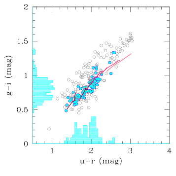
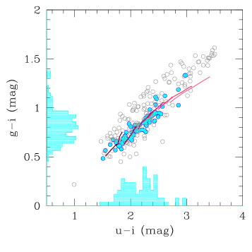
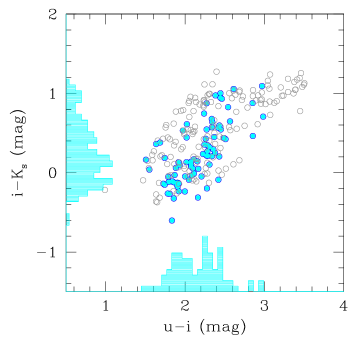
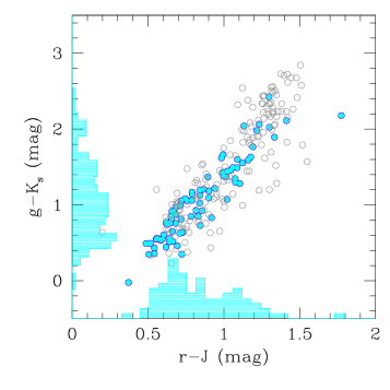
Figure 14: Color-color diagrams for the bona fide and uncertain samples of GCs, shown with blue filled dots and empty gray circles, respectively. The (arbitrarily scaled) histograms reported on the axes refer to the bona fide sample. For optical colors, the SPoT SSP models are also shown with lines as in Figure 4.

However, the $S_{N}$ versus $M_{V}$ relation has a substantial scatter. For example, from the database by Harris et al. (2013), it can be seen that galaxies with $M_{V}=-21\pm 0.2$ mag have a median population of $\sim 450$ GCs with minimum at $\sim 40$ and a maximum of $\sim 7.000$. It is worth emphasizing that, based on previous literature (Blecha, 1986; Olsen et al., 2004), Harris et al. (2013) estimates the size of the GC system of NGC 253 to be $N_{GC}=90\pm 40$. If only galaxies with morphological classes and magnitudes similar to NGC 253 are drawn from the Harris et al. (2013) sample, the median is $N_{GC}\sim 80$. The two galaxies with closest morphological class and total magnitude to NGC 253 (M 101 and NGC 6956) have a total population of detected GCs with $N_{GC}\sim 90\pm 40$ and $150\pm 40$, which is consistent with the total (coverage corrected) population we estimated.

Inspecting the radial profiles shown in Figure 13, we note a slight enhancement of GCs density at $r_{gal}\sim 25$ kpc. Although the estimated errors are relatively high, such enhancement roughly corresponds to the radial distance of the feature first found and discussed by Greggio et al. (2014), identified as a possible stellar stream remnant. However, we must highlight that our radial profile is derived from the azimuthal average of GC counts, while the RGB star counts excess found in Greggio et al. (2014) is specifically located on the northwestern side of the galaxy.

4.4 Color bimodality

A further typical element of discussion in extragalactic GC systems is the color distribution. In particular, the presence of a nearly universal color bimodality in GC systems, and the astrophysical processes underlying such ubiquitous feature, have generated a prolific and still open debate in the last decade (Spitler et al., 2006; Yoon et al., 2006; Cantiello & Blakeslee, 2007; Chies-Santos et al., 2012; Usher et al., 2012; Brodie et al., 2014; Cantiello et al., 2014). We adopted the bona fide sample, to verify the presence of color bimodality (i.e., to identify two well-separated blue and red peaks) and to estimate the differences between the two GC subpopulations in terms of the color distributions. To do so, we used the Gaussian mixture modeling code (GMM; Muratov & Gnedin, 2010). The GMM code uses the likelihood-ratio test to compare the goodness of fit for double-Gaussian versus a single-Gaussian. For the best-fit double model, it estimates the means and widths of the two components, their separation DD in terms of combined widths, and the kurtosis of the overall distribution. Values of DD larger than $\sim 2$, and negative kurtosis are necessary but not sufficient conditions for bimodality. Also, GMM provides uncertainties based on bootstrap resampling. In addition, the GMM analysis provides the positions, relative widths, and fraction of objects associated with each peak.

Inspecting the results reported in Table 3 (upper section of the table), GMM analysis shows that our bona fide GCs sample is poorly fitted by two-Gaussian distributions in most of the inspected colors. This is testified by either the high $p$-values (Cols. 10-12 in the table), the changing fractions of red GCs ($f_{2}$) when different colors are used, the positive kurtosis or the low values for the peak separation estimator (DD).

Table 3: Results of GMM runs

Color	Peak1	Peak2	$\sigma$1	$\sigma$2	$N_{GC}$	$f_{2}$	DD	Kurtosis	$p(\chi^{2})$	$p(DD)$	$p(kurt)$	bi?
(1)	(2)	(3)	(4)	(5)	(6)	(7)	(8)	(9)	(10)	(11)	(12)	(13)
$u{-}i$	1.84 $\pm$ 0.14	2.20 $\pm$ 0.29	0.08 $\pm$ 0.07	0.30 $\pm$ 0.10	81	0.88	1.62	-0.04	0.525	0.73	0.675	N
$g{-}i$	0.79 $\pm$ 0.06	1.22 $\pm$ 0.19	0.13 $\pm$ 0.04	0.11 $\pm$ 0.05	81	0.05	3.44	0.93	0.050	0.14	0.974	Y?
$u{-}r$	1.59 $\pm$ 0.09	1.97 $\pm$ 0.13	0.12 $\pm$ 0.04	0.23 $\pm$ 0.06	81	0.81	2.06	-0.09	0.634	0.61	0.630	N
$i{-}k$	0.03 $\pm$ 0.10	0.63 $\pm$ 0.21	0.23 $\pm$ 0.07	0.26 $\pm$ 0.10	82	0.35	2.49	-0.59	0.063	0.42	0.157	Y?
$r{-}j$	0.65 $\pm$ 0.04	0.95 $\pm$ 0.12	0.08 $\pm$ 0.03	0.25 $\pm$ 0.06	81	0.64	1.62	0.77	0.004	0.74	0.961	N
$g{-}k$	0.55 $\pm$ 0.14	1.19 $\pm$ 0.30	0.12 $\pm$ 0.09	0.49 $\pm$ 0.12	81	0.79	1.79	-0.35	0.026	0.70	0.378	Y?
$r{-}i$	0.22 $\pm$ 0.02	0.29 $\pm$ 0.03	0.03 $\pm$ 0.01	0.06 $\pm$ 0.01	82	0.68	1.41	0.42	0.075	0.83	0.895	N
$j{-}k$	-0.37 $\pm$ 0.06	-0.03 $\pm$ 0.08	0.18 $\pm$ 0.03	0.05 $\pm$ 0.04	82	0.10	2.53	-0.45	0.226	0.42	0.271	N
Without the red GCs
$g{-}i$	0.67 $\pm$ 0.05	0.87 $\pm$ 0.05	0.07 $\pm$ 0.02	0.09 $\pm$ 0.02	76	0.61	2.39	-0.70	0.444	0.48	0.086	N
$u{-}i$	1.94 $\pm$ 0.06	2.36 $\pm$ 0.04	0.18 $\pm$ 0.03	0.11 $\pm$ 0.03	78	0.43	2.77	-0.91	0.024	0.31	0.013	Y
$u{-}r$	1.71 $\pm$ 0.06	2.07 $\pm$ 0.03	0.17 $\pm$ 0.03	0.08 $\pm$ 0.03	77	0.41	2.67	-0.97	0.005	0.34	0.006	Y
$i{-}k$	0.04 $\pm$ 0.09	0.56 $\pm$ 0.13	0.23 $\pm$ 0.06	0.13 $\pm$ 0.06	74	0.23	2.80	-0.70	0.208	0.32	0.081	Y?
$r{-}j$	0.70 $\pm$ 0.04	1.07 $\pm$ 0.08	0.13 $\pm$ 0.03	0.07 $\pm$ 0.04	74	0.25	3.47	-0.95	0.004	0.14	0.012	Y
$g{-}k$	0.82 $\pm$ 0.12	1.51 $\pm$ 0.17	0.32 $\pm$ 0.10	0.14 $\pm$ 0.09	73	0.19	2.83	-0.85	0.136	0.29	0.032	Y?
$r{-}i$	0.23 $\pm$ 0.01	0.32 $\pm$ 0.01	0.04 $\pm$ 0.01	0.01 $\pm$ 0.01	74	0.25	3.10	-0.97	0.004	0.22	0.011	Y
$j{-}k$	-0.44 $\pm$ 0.10	-0.22 $\pm$ 0.06	0.15 $\pm$ 0.04	0.09 $\pm$ 0.03	72	0.26	1.74	-0.35	0.705	0.71	0.395	N

Table 4: Results of GMM runs for the three Gaussian model

Color	Peak1 ($N_{GC}$, $\sigma$)	Peak2 ($N_{GC}$, $\sigma$)	Peak3 ($N_{GC}$, $\sigma$)	DD	Kurtosis	$p(\chi^{2})$	$p(DD)$	$p(kurt)$
$u{-}i$	1.94 ( 43.70 , 0.19 )	2.36 ( 33.30 , 0.12 )	2.92 ( 4.00 , 0.06 )	2.73	-0.04	0.024	0.351	0.675
$g{-}i$	0.69 ( 39.10 , 0.08 )	0.88 ( 30.20 , 0.06 )	1.07 ( 11.60 , 0.17 )	2.54	0.93	0.111	0.511	0.974
$u{-}r$	1.71 ( 45.40 , 0.17 )	2.07 ( 31.60 , 0.08 )	2.53 ( 4.00 , 0.05 )	2.67	-0.09	0.002	0.459	0.630
$i{-}k$	0.04 ( 56.80 , 0.23 )	0.56 ( 16.60 , 0.12 )	0.96 ( 8.60 , 0.08 )	2.80	-0.59	0.071	0.345	0.157
$r{-}j$	0.67 ( 44.60 , 0.11 )	1.04 ( 35.40 , 0.17 )	1.77 ( 1.00 , 0.04 )	2.61	0.77	0.002	0.470	0.961
$g{-}k$	0.69 ( 43.00 , 0.25 )	1.33 ( 30.40 , 0.26 )	2.09 ( 7.60 , 0.16 )	2.49	-0.35	0.122	0.581	0.597
$r{-}i$	0.23 ( 53.40 , 0.04 )	0.32 ( 16.10 , 0.01 )	0.36 ( 12.50 , 0.06 )	3.15	0.42	0.047	0.221	0.895
$j{-}k$	0.44 ( 53.20 , 0.15 )	-0.24 ( 14.20 , 0.04 )	-0.03 ( 14.50 , 0.07 )	1.87	-0.45	0.474	0.618	0.271

We also run GMM in three Gaussian peaks mode. The results, reported in Table 4, are more satisfactory than the previous, as testified by the generally lower $p$-values. The presence of a third color peak is also visible as a red tail of GCs in the panels of Figure 14. The very red candidates are scattered around the frame, i.e., they are not sources close to the galaxy disk and reddened by the dust. In the Figure we report the color-color diagrams, together with color histograms for various colors and for the bona fide GCs sample. Taking advantage of the results on the presence of such third peak, we rerun GMM in double Gaussian mode after rejecting the candidate GCs in the third reddest peak; GMM also provides as output a table with the probability membership of each GCs to one of the fitted Gaussian. The GMM results of such a culled best sample, again with a two Gaussian model, are presented in the lower section of Table 3.

Although the new GMM results for the selected GCs sample appear, with respect to the full bona fide sample, more consistent with a bimodal-color scenario there is no homogeneity of the various inspected colors, as color bimodality is not coherently observed in all colors. In this respect, then, NGC 253 should certainly not be considered a galaxy with a bimodal GC population, showing coherent and consistent color bimodality.

5 Conclusions

We summarize the conclusion of the present work, dedicated to the definition of an updated catalog of GC candidates in NGC 253, as follows:

• The adoption of an even richer collection of color, photometric, and morphologic parameters make the selection of GC candidates more robust, but does not guarantee the complete removal of all contaminants.

• Depending on the spatial resolution of the imaging data used, for sources close enough, such as the galaxy studied here, the foreground MW stars can be separated from GCs, as the latter appear extended, with FWHM definitely larger than a point source. In cases such as that presented here, background galaxies are the primary source of contamination.

• About 10 of our candidates were already photometrically selected as GC candidates by other authors. Conversely, the largest portion of GC candidates with photometric selection in the literature are mostly identified as stars in our sample.

• Even the adoption of the $uiK_{s}$ diagram, which proved to be extremely efficient in Muñoz et al. (2014) to identify GCs in the Virgo galaxy cluster, does not ensure a clean sample of GCs.

• Spectroscopy by itself is not sufficient to define a contamination-free GC sample. In both the spectroscopic catalogs we adopted as reference, we found GCs that in our analysis are rather classified as contaminants: two background galaxies for Beasley & Sharples (2000) catalog and two foreground stars for Olsen et al. (2004) catalog. This is equivalent to a level of $\sim 20\%$ contamination in the full sample of spectroscopically confirmed GCs.

• We estimate a total population of $\sim 100$ GC, such a value should be regarded as a lower limit. The literature data for a couple of galaxies similar in morphology and luminosity to NGC 253 show that they have similar populations of detected GCs.

• The LF of bona fide sample does not show the typical symmetry around the GCLF $M^{TOM}$ peak. A fraction of bright GCs might be undetected because of large galactocentric radii or because these GCs are along the line of sight of the dusty disk. We do not have a clear explanation for the missing bright candidates. However, our results support previous studies that found evidence for recent interactions for NGC 253. Hence, one possible explanation of the observed LF might be the presence of a fraction of intermediate age, $t\sim 6$ Gyr, GCs contaminating the population of old GCs.

• The radial profile and color distributions of our bona fide GC sample show properties similar to other well-studies galaxies, i.e., a radial profile fit by a $r^{1/4}-law$.

• As for color bimodality, the statistical preference of bimodal over unimodal color distribution is not strong because this bimodality is evident with some colors and not in others.

• Finally, we provide an updated list of candidate GCs.

Moreover, as a byproduct of our analysis, thanks to the very wide wavelength interval of imaging data used, in addition to GCs we have been able to identify and distinguish the sequences of stars and the (various classes of) background galaxies (see Appendix).

The GCs in NGC 253, will be an interesting target for next generation large aperture, $\geq$30m-class telescopes, supported by adaptive optics modules that will facilitate reaching the diffraction limit.

We take as an example the MICADO/MAORY configuration at the E-ELT (Diolaiti et al., 2016; Davies et al., 2016), which has an expected optimal resolution limit of $\sim 10$mas at near-IR wavelengths; i.e., $\sim 5-10$ times better than ACS and WFC3 on board HST and the forthcoming NIRCAM on JWST; with very high Strehl ratios on a field of view of $\sim 20\arcsec$ in the case of SCAO, the instrument will allow for the first time the study of the resolved color-magnitude diagrams of stars in the GCs in the Sculptor group. Our work is an effort to provide a large census of GCs in NGC 253, which is the brightest galaxy in the group.

Appendix A Color-color diagrams

The large wavelength coverage of our dataset provides enough leverage for evidencing the presence of several sequences in the color-color diagrams inspected. Because of the different properties of the observed targets, some sequences merge or are relatively well separated with respect to others, depending on the color-color plane inspected. Using the same color-color selection procedure described in Section 3 for selecting GC candidates, we derived the approximate loci of the various sequences observed in the color-color diagrams. As an example, candidate stars were identified from the $uiK_{s}$ diagram. Then, the identified stars were analyzed in other color-color panels, and all sources scattered around the sequence were removed from the list. In a similar way, we identified the loci for passive galaxies (red early-type candidates), blue galaxies (e.g., spirals), star-forming (e.g., irregular galaxies) beyond the stellar and GCs loci. A selection of the color-color diagrams used is reported in Figure 15. In the figure we plot full sample of matched sources (black dots), and highlight with different colors five different sequences: orange, gray, red, light blue, blue filled circles indicate, respectively, the approximate loci of GCs, MW stars, passive galaxies, blue galaxies, and star-forming galaxies. To show how sequences appear before separating these sequences, we also plotted one of the color-color panels, $(g{-}K_{S})$ versus $(u{-}i)$ , with and without the sequences defined. Also, to highlight the limits of color selection when a narrow range of wavelengths is available, the third panel in the lower row shows the sequences for the $g{-}i$ versus $g{-}r$ diagram.

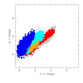
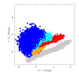
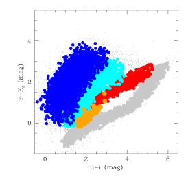
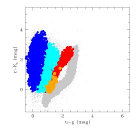
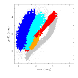
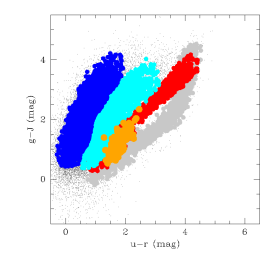
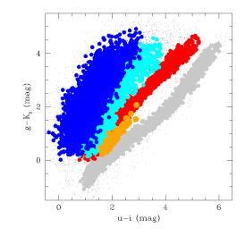
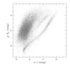
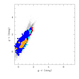
Figure 15: Color-color diagrams with the various sequences highlighted in different colors. The full sample of matched sources is indicated with black dots. Orange, gray, red, light blue, and blue dots indicate the approximate loci of GCs, MW stars, passive galaxies, blue galaxies, and star-forming galaxies. The left and middle panels in the lowermost row show the same color-color diagram, although in the second row we do not use colors for the sequences identified. The total overlap of the identified sequences in the lower right panel is notable.