Linear Programming Based Optimality Conditions and Approximate Solution of a Deterministic Infinite Horizon Discounted Optimal Control Problem in Discrete Time

Abstract.

It has been recently established that a deterministic infinite horizon discounted optimal control problem in discrete time is closely related to a certain infinite dimensional linear programming problem and its dual, the latter taking the form of a certain max-min problem. In the present paper, we use these results to establish necessary and sufficient optimality conditions for this optimal control problem and to investigate a way how the latter can be used for the construction of a near optimal control.

Vladimir Gaitsgory

Department of Mathematics, Macquarie University,

Macquarie Park, NSW 2113, Australia

Alex Parkinson

Department of Mathematics, Macquarie University,

Macquarie Park, NSW 2113, Australia

Ilya Shvartsman^∗

Department of Mathematics and Computer Science, Penn State Harrisburg,

Middletown, PA 17057, USA

(Communicated by the associate editor name)

1. Introduction and Preliminaries

It has been established that a deterministic infinite horizon discounted optimal control problem in discrete time (for brevity, we will refer to this as just the OC problem) is closely related to an infinite dimensional (ID) linear programming (LP) problem and its dual, the latter taking the form of a certain max-min problem (see [17] and also [26] for earlier developments in the Markov Decision Processes setting). In the present paper, we use results of [17] to establish necessary and sufficient optimality conditions for this optimal control problem and to investigate a way how the latter can be used for the construction of a near optimal control.

Note that necessary optimality conditions in the form of Pontryagin’s maximum principle are generally not available for discrete time optimal control problems, this being related to the fact that the so called relaxed (measure valued) controls play no role in dealing with such problems. While the classic control relaxation technique is not applicable in discrete time, a different relaxation approach based on using occupational measures generated by controls and the corresponding solutions of the dynamical system can be used in both continuous and discrete time. Such occupational measures relaxation makes it possible to reformulate the OC problem as an IDLP problem which has a nice dual counterpart, and it is the relationships between this IDLP problem and its dual that lead to the optimality conditions established in the paper.

The linear programming (LP) approach to optimal control problems has been studied extensively in both stochastic and deterministic settings (see, e.g., [6], [9], [10], [14],[25], [29], [33], [34] and, respectively, [1], [13], [15], [18], [19], [20], [22], [27], [28], [30], [31], [32], [36] as well as references therein). In particular, results establishing the validity of LP formulations of deterministic infinite horizon OC problems with time discounting have been obtained in [18], [19] and [27] for systems evolving in continuous time and in [16] and [17] for systems evolving in discrete time. (Note that other approaches/techniques for dealing with deterministic optimal control problems on the infinite time horizon have been studied, e.g., in [4], [8], [11], [23], [24], [37], [38] and [39]; see also references therein.) In this paper, we continue the line of research started in [16] and [17].

Consider the control system

$$y(t+1)=f(y(t),u(t)),\ \;t\in{\mathcal{T}}:=\{0,1,\dots\ \},$$ (1)

$$y(0)=y_{0},$$

$$y(t)\in Y,$$

$$u(t)\in U(y(t)),$$

where $Y$ is a given nonempty compact subset of $I\!\!R^{m}$, $\ U(\cdot):\,Y\leadsto U_{0}$ is an upper semicontinuous compact-valued mapping to a given compact metric space $U_{0}$, $\ f(\cdot,\cdot):\,I\!\!R^{m}\times U_{0}\to I\!\!R^{m}$ is a continuous function. A control $u(\cdot)$ and the pair $(y(\cdot),u(\cdot))$ are called an admissible control and, respectively, an admissible process if the relationships (1) are satisfied. The set of all admissible controls is denoted as ${\mathcal{U}}(y_{0})$.

Everywhere in what follows, we will be dealing with the optimal control problem

$$\inf_{u(\cdot)\in{\mathcal{U}}(y_{0})}\sum_{t=0}^{\infty}\alpha^{t}g(y(t),u(t))=:V(y_{0}),$$ (2)

where $g:\,I\!\!R^{m}\times U_{0}\to I\!\!R^{m}$ is a continuous function and $\alpha\in(0,1)$ is a discount factor. Note that the last two constraints in (1) can be rewritten as one:

$$u(t)\in A(y(t)),$$

where the map $\ A(\cdot):\,Y\leadsto U_{0}$ is defined by the equation

$$A(y):=\{u\in U(y)|\,f(y,u)\in Y\}\ \ \ \forall y\in Y.$$ (3)

Note also that from the fact that $U(\cdot)$ is upper semicontinuous and $\ f(\cdot,\cdot)$ is continuous it follows that the map $A(\cdot)$ is upper semicontinuous and its graph $G$,

$$G:={\rm graph}\,A=\{(y,u)|\,y\in Y,\,u\in U(y),\,f(y,u)\in Y\},$$

is a compact subset of $Y\times U_{0}$.

The standing assumption in the paper is the following

ASSUMPTION I: The set $A(y)$ is not empty for any $y\in Y$.

As can be readily seen, this assumption implies that the set ${\mathcal{U}}(y)$ is not empty for any $y\in Y$ (systems satisfying such a property are called viable; see [3]). It can be shown (see, e.g., [5] or [17]) that under this assumption an optimal solution of problem (1) exists, the optimal value function $V(\cdot)$ is lower semicontinuous and bounded on $Y$, and $V(\cdot)$ is a solution of the following equation (the dynamic programming principle)

$$V(y)=\min_{u\in A(y)}\{g(y,u)+\alpha V(f(y,u))\}\ \ \ \ \forall y\in Y.$$ (4)

Note that this equation can be rewritten in the form that resembles the Hamilton-Jacobi-Bellman equation for continuous time systems:

$$H_{V}(y)-(1-\alpha)V(y)=0\ \ \ \ \ \forall y\in Y,$$ (5)

where, for any lower semicontinuous function $\psi:\,Y\to I\!\!R$,

$$H_{\psi}(y):=\min_{u\in A(y)}\{g(y,u)+\alpha(\psi(f(y,u))-\psi(y))\}.$$ (6)

Along with (5), let us consider the following max-min problem

$$\max_{\psi\in LS}\inf_{y\in Y}\{H_{\psi}(y)-(1-\alpha)(\psi(y)-\psi(y_{0}))\}=:\mu^{*}(y_{0})$$ (7)

where $max$ is over the class of bounded lower semicontinuous functions from $Y$ to $I\!\!R$ (denoted as $LS$). It has been recently established in [17] (see also Proposition 1 below) that the maximum in (7) is reached at $\psi=V$. Note that from the fact that $V$ is a maximizer in (7) it follows that $\tilde{V}:=V+{\rm const}$ is a maximizer in (7) as well. The set of maximizers in (7) may, in fact, be much broader than just constant shifts of the optimal value function (see an example in Section 2).

In this paper, we establish that necessary and sufficient optimality conditions for problem (2) can be stated in terms of any such maximizer. (Note that the max-min problem (7) involves the dependence on $y_{0}$ and the optimality conditions in terms of a maximizer in (7) will only be valid for the solutions satisfying the initial condition $y(0)=y_{0}$, this being in contrast to the solution of the dynamic programming equation (5), which allows to characterize the optimal solutions for arbitrary initial conditions.)

We will also indicate a way how an approximate maximizer in (7) can be used for the construction of a near optimal control for problem (2), this construction will be illustrated by a numerical example.

The paper is organized as follows. In Section 2, we establish necessary and sufficient conditions of optimality for problem (2) in terms of a maximizer in the max-min problem (7) (the main result of this section is Theorem 2.1). In Section 3, we introduce $N$-approximating max-min problem, in which in contrast to (7), the maximization is over $\psi\in D_{N}$, where $D_{N}$ is an $N$-dimensional subspace of the space of continuous functions on $Y$. We show that the optimal value of the $N$-approximating max-min problem converges to the optimal value of (7) as $N\rightarrow\infty$ (Proposition 4) and we establish that a maximizer in the $N$-approximating max-min problem exists for any $N$ under a readily verifiable controllability condition (Proposition 5). In Section 4, we establish that a maximizer in the $N$-approximating max-min problem can be used for the construction of a near optimal control (Theorem 4.1). Sections 5 and 6 are devoted to numerical examples that illustrate the latter construction. Some of the results presented in Section 2 were announced in [16] without proofs. Continuous time counterparts of results of Sections 3 and 4 can be found in [21].

To conclude this section, let us outline some notations and results that are used further in the text. For an admissible process $(y(\cdot),u(\cdot))$, a probability measure $\gamma_{u}$ is called the discounted occupational measure generated by $u(\cdot)$ if, for any Borel set $Q\subset G$,

$$\gamma_{u}(Q)=(1-\alpha)\sum_{t=0}^{\infty}\alpha^{t}1_{Q}(y(t),u(t)),$$ (8)

where $1_{Q}(\cdot)$ is the indicator function of $Q$.

It can be shown that this definition is equivalent to the validity of the relationship

$$\int_{G}q(y,u)\gamma_{u}(dy,du)=(1-\alpha)\sum_{t=0}^{\infty}\alpha^{t}q(y(t),u(t))$$ (9)

for any Borel measurable function $q$ on $G$. Indeed, (8) obviously implies the validity of for a simple function (i.e., a finite sum of indicator functions of Borel measurable sets). The validity of for an arbitrary Borel $q$ follows from the definition of the Lebesgue integral as a limit of integrals of simple functions; see, e.g. [2].

To describe convergence properties of occupational measures, we introduce the following metric on ${\mathcal{P}}(G)$ (the space of probability measures defined on Borel subsets of $G$):

$$\rho(\gamma^{\prime},\gamma^{\prime\prime}):=\sum_{j=1}^{\infty}{1\over 2^{j}}\left|\int_{G}q_{j}(y,u)\gamma^{\prime}(dy,du)-\int_{G}q_{j}(y,u)\gamma^{\prime\prime}(dy,du)\right|$$

for $\gamma^{\prime},\gamma^{\prime\prime}\in{\mathcal{P}}(G)$, where $q_{j}(\cdot),\,j=1,2,\dots,$ is a sequence of Lipschitz continuous functions dense in the unit ball of the space of continuous functions $C(G)$ from $G$ to $I\!\!R$. This metric is consistent with the weak^∗ convergence topology on ${\mathcal{P}}(G)$, that is, a sequence $\gamma^{k}\in{\mathcal{P}}(G)$ converges to $\gamma\in{\mathcal{P}}(G)$ in this metric if and only if

$$\lim_{k\to\infty}\int_{G}q(y,u)\gamma^{k}(dy,du)=\int_{G}q(y,u)\gamma(dy,du)$$

for any $q\in C(G)$. Using this metric, we can define the “distance” $\rho(\gamma,\Gamma)$ between $\gamma\in{\mathcal{P}}(G)$ and $\Gamma\subset{\mathcal{P}}(G)$ and the Hausdorff metric $\rho_{H}(\Gamma_{1},\Gamma_{2})$ between $\Gamma_{1}\subset{\mathcal{P}}(G)$ and $\Gamma_{2}\subset{\mathcal{P}}(G)$ as follows:

$$\rho(\gamma,\Gamma):=\inf_{\gamma^{\prime}\in\Gamma}\rho(\gamma,\gamma^{\prime}),\quad\rho_{H}(\Gamma_{1},\Gamma_{2}):=\max\{\sup_{\gamma\in\Gamma_{1}}\rho(\gamma,\Gamma),\sup_{\gamma\in\Gamma_{2}}\rho(\gamma,\Gamma_{2})\}.$$

Let $\Gamma(y_{0})$ denote the set of all discounted occupational measures generated by the admissible controls. That is,

$$\Gamma(y_{0}):=\bigcup_{u(\cdot)\in{\mathcal{U}}}\{\gamma_{u}\}.$$

Note that, due to Assumption I, the set $\Gamma(y_{0})$ is not empty. Also, due to (9), problem (1) can be rewritten as

$$\min_{\gamma\in\Gamma(y_{0})}\int_{G}g(y,u)\gamma(dy,du)=(1-\alpha)V(y_{0}).$$ (10)

Consider the problem

$$\min_{\gamma\in W(y_{0})}\int_{G}g(y,u)\gamma(dy,du)=:g^{*}(y_{0}),$$ (11)

where $W(y_{0})$ is the set of probability measures defined by the equation

$$W(y_{0}):=\{\gamma\in{\mathcal{P}}(G)|\,$$ (12)

$$\int_{G}[\alpha(\varphi(f(y,u))-\varphi(y))+(1-\alpha)(\varphi(y_{0})-\varphi(y))]\gamma(dy,du)=0\quad\forall\varphi\in C(Y)\}.$$

Note that (11) is an infinite dimensional linear programming problem since both the objective function and the constraints are linear with respect to the “decision variable” $\gamma$. Note also that the set $W(y_{0})$ is not empty (as follows from the statement (i) of Proposition 1 below) and, as can be readily verified, it is compact in weak^∗ topology. Hence, the minimum in (11) is reached.

In [17], it has been established that problem (7) is dual to the IDLP problem (11) and that these two problems are related to the optimal control problem (2). Some of the relationships between problems (7), (11) and (2) are summarized in the following proposition.

Proposition 1.

The following statements are valid:

(i) The closed convex hull of the set of discounted occupational measures $\Gamma(y_{0})$ is equal to the set $W(y_{0})$. That is,

$$\bar{\rm co}\,\Gamma(y_{0})=W(y_{0}).$$ (13)

(ii) The optimal values in problems (7) and (11) coincide and are equal to the optimal value in (2) multiplied by $(1-\alpha)$, that is,

$$\mu^{*}(y_{0})=g^{*}(y_{0})=(1-\alpha)V(y_{0}).$$ (14)

(iii) The supremum in (7) is reached at $\psi=V$.

Proof. The statements (ii) and (iii) follow from Theorem 4.1 in [17]. The statement (i) follows from Corollary 2 in [17]. $\Box$

2. Necessary and Sufficient Optimality Conditions

We will say that $\psi\in LS$ is a solution of (7) if

$$\inf_{y\in Y}\{H_{\psi}(y)-(1-\alpha)(\psi(y)-\psi(y_{0}))\}=\mu^{*}(y_{0}),$$ (15)

which is equivalent to

$$\inf_{(y,u)\in G}\{g(y,u)+\alpha(\psi(f(y,u))-\psi(y))+(1-\alpha)(\psi(y_{0})-\psi(y))\}=\mu^{*}(y_{0}).$$ (16)

Due to Proposition 1(iii), $V$ is a maximizer in (7), and, as has been mentioned earlier, all constant shifts of $V$ are solutions of (7) as well. As also has been mentioned above, the set of solutions of problem (7) can be significantly larger than the set of these shifts. This is demonstrated by the following example.

Example. Consider the problem

$${\rm Minimize}\,\sum_{t=0}^{\infty}\alpha^{t}g(y(t)),$$

$$y(t+1)=u(t),\,t\in{\mathcal{T}},$$

$$y(0)=y_{0},$$

$$u(t)\in[0,1],$$

$$y(t)\in[0,1],$$

where function $g$ is increasing on $[0,1]$ and $g(0)=0$.

It is clear that the optimal control is $u\equiv 0$ with the corresponding trajectory

$$y(t)=\begin{cases}y_{0},&t=0,\\ 0,&t>0,\end{cases}$$

and the value function is $V(y)=g(y)$.

Let us show that, if $\psi:\,[0,1]\to I\!\!R$ is such that $\psi(y_{0})=g(y_{0})$, $\psi(0)=g(0)=0$, and $0\leq\psi(y)\leq g(y)$ for all $y\in[0,1]$, then $\psi$ is a solution of (7). Indeed, for such $\psi$ we have

$$\min_{(y,u)\in[0,1]\times[0,1]}\{g(y)+\alpha\psi(u)-\psi(y)+(1-\alpha)\psi(y_{0})\}=(1-\alpha)\psi(y_{0})=(1-\alpha)V(y_{0}),$$

therefore, $\psi$ is a solution of (7) due to Proposition 1(ii). $\Box$

The theorem stated below establishes necessary and sufficient optimality conditions for problem (2) in terms of any solution of (7).

Theorem 2.1.

Let $\psi$ be a solution of (7). Optimality of an admissible process $(y(\cdot),u(\cdot))$ is equivalent to each of the following for all $t\in{\mathcal{T}}$:

(i)

$$(y(t),u(t))={\rm argmin}_{(y,u)\in G}\{g(y,u)+\alpha\psi(f(y,u))-\psi(y)\},$$ (17)

or, equivalently,

$$u(t)={\rm argmin}_{u\in A(y)}\{g(y(t),u)+\alpha\psi(f(y(t),u))\},$$ (18)

$$y(t)={\rm argmin}_{y\in Y}\{H_{\psi}(y)-(1-\alpha)\psi(y)\};$$

(ii)

$$\psi(y(t))=V(y(t))+\psi(y_{0})-V(y_{0}),$$ (19)

that is, $\psi$ and $V$ coincide on the optimal trajectory up to the constant $\psi(y_{0})-V(y_{0})$.

Furthermore, if $(y(\cdot),u(\cdot))$ is optimal, then

$$H_{\psi}(y(t))-(1-\alpha)\psi(y(t))=(1-\alpha)(V(y_{0})-\psi(y_{0})).$$ (20)

Proof. Since both $V$ and $\psi$ are solutions of (7), we have

$$\inf_{y\in Y}\{H_{V}(y)+(1-\alpha)(V(y_{0})-V(y))\}=\inf_{y\in Y}\{H_{\psi}(y)+(1-\alpha)(\psi(y_{0})-\psi(y))\}.$$

Taking into account that $H_{V}(y)-(1-\alpha)V(y)=0$ for all $y\in Y$ due to (5), we have

$$\inf_{y\in Y}\{H_{\psi}(y)-(1-\alpha)\psi(y)\}=(1-\alpha)(V(y_{0})-\psi(y_{0})),$$ (21)

which implies that

$$g(y,u)+\alpha\psi(f(y,u))-\psi(y)\geq(1-\alpha)(V(y_{0})-\psi(y_{0}))\quad\hbox{for all }(y,u)\in G.$$ (22)

Further, the identity

$$\sum_{t=0}^{\infty}\alpha^{t}\psi(y(t))=\psi(y_{0})+\alpha\sum_{t=0}^{\infty}\alpha^{t}\psi(f(y(t),u(t))),$$ (23)

is equivalent to

$$\sum_{t=0}^{\infty}\alpha^{t}[\alpha\psi(f(y(t),u(t)))-\psi(y(t))+(1-\alpha)\psi(y_{0})]=0.$$ (24)

Assume that $(y(\cdot),u(\cdot))$ is an optimal process. Then

$$\sum_{t=0}^{\infty}\alpha^{t}g(y(t),u(t))=V(y_{0}),$$

or, equivalently,

$$\sum_{t=0}^{\infty}\alpha^{t}[g(y(t),u(t))-(1-\alpha)V(y_{0})]=0.$$ (25)

Adding (24) and (25) we obtain

$$\sum_{t=0}^{\infty}\alpha^{t}[g(y(t),u(t))+\alpha\psi(f(y(t),u(t))-\psi(y(t))+(1-\alpha)(\psi(y_{0})-V(y_{0}))]=0.$$ (26)

Taking into account (22) we arrive at

$$g(y(t),u(t))+\alpha\psi(f(y(t),u(t)))-\psi(y(t))=(1-\alpha)(V(y_{0})-\psi(y_{0}))\quad\hbox{for all }t,$$ (27)

and (17).

Let us see that (20) holds. From the definition of $H$, (20) is equivalent to

$$\min_{u\in A(y(t))}\{g(y(t)),u)+\alpha\psi(f(y(t),u))\}-\psi(y(t))=(1-\alpha)(V(y_{0})-\psi(y_{0}))\quad\hbox{for all }t.$$

From (22) and (27) it follows that this relation holds with the minimizing $u\in A(y(t))$ equal to $u(t)$.

To prove (19) take $k\in{\mathcal{T}}$. From the identity

$$\sum_{t=k}^{\infty}\alpha^{t}\psi(y(t))=\alpha^{k}\psi(y(k))+\sum_{t=k+1}^{\infty}\alpha^{t}\psi(y(t))$$

we get

$$\alpha^{k}\psi(y(k))=\sum_{t=k}^{\infty}\alpha^{t}[\psi(y(t))-\alpha\psi(f(y(t),u(t))].$$ (28)

From optimality of $(y(\cdot),u(\cdot))$, via (27), we obtain

$$\alpha^{k}\psi(y(k)) =\sum_{t=k}^{\infty}\alpha^{t}[g(y(t),u(t))+(1-\alpha)(\psi(y_{0})-V(y_{0}))]$$ (29)

$$=\alpha^{k}\left\{\sum_{t=0}^{\infty}\alpha^{t}g(y(t+k),u(t+k))+(\psi(y_{0})-V(y_{0}))\right\}$$

$$=\alpha^{k}\{V(y(k))+\psi(y_{0})-V(y_{0})\},$$

therefore, $\psi(y(k))=V(y(k))+V(y_{0})-\psi(y_{0})$, i.e., (19) holds.

Conversely, assume that assertion (i) of the theorem is true. Let us rewrite (21) in the form

$$\inf_{y\in Y}\min_{u\in A(y)}\{g(y,u)+\alpha\psi(f(y,u))-\psi(y)\}=(1-\alpha)(V(y_{0})-\psi(y_{0})).$$

From (17) it follows that $\displaystyle\inf_{y\in Y}\min_{u\in A(y)}$ in this formula is reached when $(y,u)=(y(t),u(t))$ for all $t$, in which case (27) holds. The latter implies (26). Subtracting (24) from (26) we obtain (25), therefore, the process $(y(\cdot),u(\cdot))$ is optimal.

Assume now that (ii) holds. Similarly to formula (29), we obtain for any $k\in{\mathcal{T}}$

$$\psi(y(k))=V(y(k))+\psi(y_{0})-V(y_{0})=\sum_{t=0}^{\infty}\alpha^{t}g(y(t+k),u(t+k))+(\psi(y_{0})-V(y_{0}))$$

$$=\alpha^{-k}\left\{\sum_{t=k}^{\infty}\alpha^{t}[g(y(t),u(t))+(1-\alpha)(\psi(y_{0})-V(y_{0}))]\right\}.$$

From this equality and (28) we obtain

$$\sum_{t=k}^{\infty}\alpha^{t}[g(y(t),u(t))+(1-\alpha)(\psi(y_{0})-V(y_{0}))]=\sum_{t=k}^{\infty}\alpha^{t}[\psi(y(t))-\alpha\psi(f(y(t),u(t))],$$

wherein setting $k=0$ leads to (26). As above, subtracting (24) from (26) we get (25), that is, the process $(y(\cdot),u(\cdot))$ is optimal. The theorem is proved. $\Box$

Assertion (ii) of the theorem above states that $\psi$ and $V$ are equal on the optimal trajectory, up to the constant $\psi(y_{0})-V(y_{0})$. It can be shown that, away from the optimal trajectory, the equality becomes inequality.

Proposition 2.

Let $\psi$ be a solution of (7). Then $\psi(y)\leq V(y)+\psi(y_{0})-V(y_{0})$.

Proof. Take the optimal trajectory $(y(\cdot),u(\cdot))$ starting from an arbitrary initial condition $y_{1}$. Replacing $y_{0}$ with $y_{1}$ in (23) we get

$$\psi(y_{1})=\sum_{t=0}^{\infty}\alpha^{t}(\psi(y(t))-\alpha\psi(f(y(t),u(t)))).$$ (30)

From (22) it follows that

$$\psi(y(t))-\alpha\psi(f(y(t),u(t))\leq g(y(t),u(t))-(1-\alpha)(V(y_{0})-\psi(y_{0})).$$

Taking into account (30) and the latter inequality we obtain

$$\psi(y_{1})\leq\sum_{t=0}^{\infty}\alpha^{t}g(y(t),u(t))-(V(y_{0})-\psi(y_{0}))=V(y_{1})-(V(y_{0})-\psi(y_{0})),$$

and the assertion of the proposition follows. $\Box$

Remark. If we introduce the function resembling the unmaximized Hamiltonian

$${\mathcal{H}}_{\psi}(y,u):=\alpha(\psi(f(y,u))-\psi(y))+g(y,u),$$

then the first of the conditions (18) can be written in the form resembling the Pontryagin-type minimum principle

$$u(t)={\rm argmin}_{u\in A(y)}\,{\mathcal{H}}_{\psi}(y(t),u).$$

(Of course, it is well known that the Pontryagin maximum principle doesn’t hold in general for discrete time systems without additional convexity assumptions.)

Let us complete this section with another characterization of the solution set of the max-min problem (7). Consider the inequality (compare with (5))

$$H_{\psi}(y)-(1-\alpha)\psi(y)\geq 0\ \ \ \ \ \forall y\in Y.$$ (31)

The following result establishes the relationships between the solutions of this inequality satisfying the additional condition

$$\psi(y_{0})=V(y_{0})$$ (32)

and the solutions of the max-min problem (7).

Proposition 3.

If $\psi\in LS$ is a solution of inequality (31) satisfying (32), then $\psi$ is a solution of the max-min problem (7). Conversely, if $\psi$ is a solution of the max-min problem (7), then

$$\tilde{\psi}(y):=\psi(y)-\psi(y_{0})+V(y_{0}),$$ (33)

is a solution of inequality (31) satisfying (32).

Proof. Let $\psi\in LS$ be a solution of inequality (31) satisfying (32). Then, by (14),

$$H_{\psi}(y)-(1-\alpha)(\psi(y)-\psi(y_{0}))\geq(1-\alpha)\psi(y_{0})=(1-\alpha)V(y_{0})=\mu^{*}(y_{0})\ \ \ \ \ \forall y\in Y.$$

The latter implies (15) due to the definition of $\mu^{*}(y_{0})$ (see (7)). Hence, $\psi$ is a solution of the max-min problem (7).

Let now $\psi$ be a solution of the max-min problem (7). Then $\tilde{\psi}$ defined in (33) will be a solution of this problem too. Also, $\tilde{\psi}$ will satisfy (32) ($\tilde{\psi}(y_{0})=V(y_{0})$). Consequently, by (14),

$$H_{\tilde{\psi}}(y)-(1-\alpha)(\tilde{\psi}(y)-\tilde{\psi}(y_{0}))\geq\mu^{*}(y_{0})=(1-\alpha)V(y_{0})=(1-\alpha)\tilde{\psi}(y_{0})$$

$$\Rightarrow\ \ \ \ \ \ H_{\tilde{\psi}}(y)-(1-\alpha)\tilde{\psi}(y))\geq 0\ \ \ \ \ \forall y\in Y.$$

That is, $\tilde{\psi}$ is a solution of inequality (31) as well. $\Box$

3. $N$-Approximating Max-Min Problem

Let $\{\phi_{i}\}_{i=1}^{\infty}$ be a sequence of continuous functions with the following properties:

(i) Any finite collection of functions from this sequence is linearly independent on any open set;

(ii) For any $\psi\in C(Y)$ (the space of continuous functions on $Y$) and any $\delta>0$, there exist $N$ and $\lambda_{i}^{N}$, $i=1,\dots,N$ such that $\displaystyle\max_{y\in Y}|\psi(y)-\sum_{i=1}^{N}\lambda_{i}^{N}\phi_{i}(y)|\leq\delta$.

Note that, due to the “approximation property” (ii), the set $W(y_{0})$ defined in (12) can be rewritten in the form

$$W(y_{0}):=\{\gamma\in{\mathcal{P}}(G)|\,$$ (34)

$$\int_{G}[\alpha(\varphi_{i}(f(y,u))-\varphi_{i}(y))+(1-\alpha)(\varphi_{i}(y_{0})-\varphi_{i}(y))]\gamma(dy,du)=0\quad\forall\ i=1,...\}.$$

In what follows it is assumed that $\phi_{1}\equiv 1$. Hence, the linear independence property (i) implies that

$$\sum_{i=1}^{N}v_{i}\phi_{i}(y)=\hbox{const}\ \ \ \forall y\in Q\ \ \ \ \ \Leftrightarrow\ \ \ \ v_{i}=0\ \forall\ i=1,\dots,N$$ (35)

if $Q$ has a nonempty interior. (An example of a sequence with the properties (i) and (ii) is the sequence of monomials $y_{1}^{i_{1}}\dots y_{m}^{i_{m}},\,i_{1},\dots,i_{m}=0,1,\dots$, where $y_{j}$ stands for the $j$th component of $y$.)

Consider the max-min problem

$$\sup_{\psi\in D_{N}}\min_{(y,u)\in G}\{g(y,u)+\alpha(\psi(f(y,u))-\psi(y))+(1-\alpha)(\psi(y_{0})-\psi(y))\}=:\mu_{N}^{*}(y_{0}),$$ (36)

where $D_{N}\subset C(Y)$ is the finite dimensional space defined by the equation

$$D_{N}:=\{\psi\in C(Y)|\,\psi(y)=\sum_{i=1}^{N}\lambda_{i}\phi_{i}(y);\ \lambda_{i}\in I\!\!R,\,i=1,\dots,N\}.$$

Problem (36) is referred to as the $N$-approximating problem.

Proposition 4.

The optimal value $\mu_{N}^{*}(y_{0})$ of the $N$-approximating problem converges to the optimal value $\mu^{*}(y_{0})$ of problem (7) as $N$ tends to infinity. That is,

$$\lim_{N\to\infty}\mu^{*}_{N}(y_{0})=\mu^{*}(y_{0}).$$

Proof. Let

$$\mu_{C}^{*}(y_{0}):=\sup_{\psi\in C(Y)}\min_{(y,u)\in G}\{g(y,u)+\alpha(\psi(f(y,u))-\psi(y))+(1-\alpha)(\psi(y_{0})-\psi(y))\},$$ (37)

where sup is over the space of continuous functions. It is obvious that $\mu^{*}_{N}(y_{0})\leq\mu_{C}^{*}(y_{0})\ \forall N$. Also the sequence $\{\mu^{*}_{N}(y_{0})\}$ is monotone increasing. Hence, the limit $\displaystyle\lim_{N\to\infty}\mu^{*}_{N}(y_{0})$ exists and does not exceed $\mu_{C}^{*}(y_{0})$. Also, from the approximating property of $\{\phi_{i}\}$ it follows, in fact, that $\displaystyle\lim_{N\to\infty}\mu^{*}_{N}(y_{0})=\mu_{C}^{*}(y_{0})$. Thus, to prove the proposition, it is sufficient to establish that $\mu_{C}^{*}(y_{0})$ is equal to $\mu^{*}(y_{0})$. This is established by the lemma stated below. $\Box$

Lemma 3.1.

The equality

$$\mu_{C}^{*}(y_{0})=\mu^{*}(y_{0})$$ (38)

is valid.

Proof. Since

$$\mu_{C}^{*}(y_{0})\leq\mu^{*}(y_{0}),$$ (39)

it is sufficient to establish that the inequality $\mu_{C}^{*}(y_{0})\geq\mu^{*}(y_{0})$ holds true.

To prove the latter, note first that for any $\psi\in C(Y)$, we have

$$\min_{(y,u)\in G}\{\alpha(\psi(f(y,u))-\psi(y))+(1-\alpha)(\psi(y_{0})-\psi(y))\}\leq 0.$$ (40)

Indeed, if this was not the case, then, for $\psi_{m}:=m\psi$ with positive integer $m$ we would get

$$\lim_{m\to\infty}\min_{(y,u)\in G}\{g(y,u)+\alpha(\psi_{m}(f(y,u))-\psi_{m}(y))+(1-\alpha)(\psi_{m}(y_{0})-\psi_{m}(y))\}=+\infty,$$

contradicting the fact that $\mu_{C}^{*}$ is bounded (the latter being implied by (39)).

Assume that functions $\{\phi_{i}\}$ are normalized so that $\max_{y\in Y}|\phi_{i}(y)|<1/2^{i}$. Define $\hat{Q}\subset I\!\!R\times l_{1}$ by

$$\hat{Q}:=\{(\theta,x)|\,\theta\geq\int_{G}g(y,u)\gamma(dy,du),\,x=\left(x_{1},x_{2},\dots\right),$$

$$x_{i}=\int_{G}[\alpha(\phi_{i}\left(f\left(y,u\right)\right)-\phi_{i}\left(y\right))+\left(1-\alpha\right)(\phi_{i}\left(y_{0}\right)-\phi_{i}\left(y\right))]\gamma\left(dy,du\right),\,\gamma\in\mathcal{P}(G)\}.$$

It’s easy to see that the set $\hat{Q}$ is a closed subset of $I\!\!R\times l_{1}$ and that, for any $j=1,2,\dots$, the point $(g^{*}(y_{0})-\frac{1}{j},0)$ does not belong to $\hat{Q},$ where 0 is the zero element of $l_{1}$ (otherwise, $g^{*}(y_{0})$ is not the minimum value in (11)). Due to Hahn-Banach separation theorem (see, e.g., [12], Section V.2) there exists a sequence $(\kappa^{j},\lambda^{j})\in I\!\!R\times l^{\infty}$ (where $\lambda^{j}=(\lambda_{1}^{j},\lambda_{2}^{j},\dots)$) such that

$$\kappa^{j}\left(g^{*}(y_{0})-\frac{1}{j}\right)+\delta^{j}\leq\inf_{(\theta,x)\in\hat{Q}}\{\kappa^{j}\theta+\sum_{i=1}^{\infty}\lambda_{i}^{j}x_{i}\}$$ (41)

$$=\inf_{\gamma\in\mathcal{P}(G)}\{\kappa^{j}\theta+\int_{G}[\alpha(\psi_{\lambda^{j}}(f(y,u))-\psi_{\lambda^{j}}(y))+(1-\alpha)(\psi_{\lambda^{j}}(y_{0})-\psi_{\lambda^{j}}(y))]\gamma(dy,du)$$

$$s.t.\,\theta\geq\int_{G}g(y,u)\gamma(dy,du)\},$$

where $\delta^{j}>0$ for all $j$ and $\psi_{\lambda^{j}}:=\sum_{i=1}^{\infty}\lambda_{i}^{j}\phi_{i}$. From the last formula it is easy to see that $\kappa^{j}\geq 0$. Let us show that, actually, $\kappa^{j}>0$. Indeed, if it was not the case and $\kappa^{j}=0$, then we would have

$$0<\delta^{j}\leq \min_{\gamma\in\mathcal{P}(G)}\int_{G}[\alpha(\psi_{\lambda^{j}}(f(y,u))-\psi_{\lambda^{j}}(y))+(1-\alpha)(\psi_{\lambda^{j}}(y_{0})-\psi_{\lambda^{j}}(y))]\gamma(dy,du)$$

$$= \min_{(y,u)\in G}\{(\alpha(\psi_{\lambda^{j}}(f(y,u))-\psi_{\lambda^{j}}(y))+(1-\alpha)(\psi_{\lambda^{j}}(y_{0})-\psi_{\lambda^{j}}(y))\},$$

which is a contradiction to (40). Thus, $\kappa^{j}>0$. Dividing (41) by $\kappa_{j}$, we obtain

$$g^{*}(y_{0})-\frac{1}{j} <\min_{\gamma\in{\mathcal{P}}(G)}\{\int_{G}\big{(}g(y,u)+{1\over\kappa^{j}}(\alpha(\psi_{\lambda^{j}}(f(y,u))-\psi_{\lambda^{j}}(y))$$

$$+(1-\alpha)(\psi_{\lambda^{j}}(y_{0})-\psi_{\lambda^{j}}(y))\big{)}\gamma(dy,du)\}$$

$$=\min_{(y,u)\in G} \{g(y,u)+{1\over\kappa^{j}}(\alpha(\psi_{\lambda^{j}}(f(y,u))-\psi_{\lambda^{j}}(y))+(1-\alpha)(\psi_{\lambda^{j}}(y_{0})-\psi_{\lambda^{j}}(y)))\}$$

$$\leq\mu^{*}_{C}(y_{0})$$ .

Therefore, $g^{*}(y_{0})\leq\mu^{*}_{C}(y_{0})$. Taking into account that, due to Proposition 1, $g^{*}(y_{0})=\mu^{*}(y_{0})$, we obtain $\mu^{*}(y_{0})\leq\mu^{*}_{C}(y_{0})$. This, along with (39), proves the (38). $\Box$

A function $\psi\in D_{N}$ will be called a solution of the $N$-approximating problem (36) if

$$\min_{(y,u)\in G}\{g(y,u)+\alpha(\psi(f(y,u))-\psi(y))+(1-\alpha)(\psi(y_{0})-\psi(y))\}=\mu_{N}^{*}(y_{0}).$$ (42)

From Proposition 4 it follows that, if $\psi\in D_{N}$ is a solution of (36), then it solves the max-min problem (7) approximately in the sense that (compare with (15)

$$\min_{y\in Y}\{H_{\psi}(y)-(1-\alpha)(\psi(y)-\psi(y_{0}))\}=\mu^{*}(y_{0})-\kappa_{N},$$

where $\kappa_{N}:=\mu^{*}(y_{0})-\mu_{N}^{*}(y_{0})\rightarrow 0$ as $N\rightarrow\infty$. Below we establish that a solution of the $N$-approximating problem exists for any $N$ under a readily verifiable controllability-type assumption.

Let ${\mathcal{R}}_{y_{0}}$ be the reachable set for system (1) in finite time. That is,

$${\mathcal{R}}_{y_{0}}:=\{y\ |\ y=y(t)\ \ {\rm for\ some\ solution\ of\ (\ref{A1})}\ {\rm and\ for\ some}\ t\in{\mathcal{T}}\}.$$

Proposition 5.

Assume that

$${\rm int}\,({\rm cl}\,{\mathcal{R}}_{y_{0}})\neq\emptyset.$$ (43)

Then a solution of the $N$-approximating problem exists for any $N$.

Proof. Let us show first that the only function $\psi\in D_{N}$ satisfying the inequality

$$\alpha({\psi}(f(y,u))-{\psi}(y))+(1-\alpha)({\psi}(y_{0})-{\psi}(y))\geq 0\,\,\ \ \ \forall\ (y,u)\in G,$$ (44)

is $\psi\equiv 0$. Indeed, rewrite this inequality as

$$\alpha{\psi}(f(y,u))-{\psi}(y)+(1-\alpha){\psi}(y_{0})\geq 0\,\,\ \ \ \forall\ (y,u)\in G.$$

Let $(y(\cdot),u(\cdot))$ be an admissible process in (1). It follows from this inequality and (24) that each term in (24) is equal to zero, that is,

$$0 =\alpha\psi(f(y(t),u(t))-\psi(y(t))+(1-\alpha)\psi(y_{0})$$

$$=\alpha(\psi(y(t+1))-\psi(y(t)))+(1-\alpha)(\psi(y_{0})-\psi(y(t))).$$

Hence,

$$\psi(y(t+1))-\psi(y(t))={1-\alpha\over\alpha}(\psi(y(t))-\psi(y_{0}))\quad\ \forall t\in{\mathcal{T}}.$$

As can be readily verified, the latter implies $\psi(y(t))\equiv\psi(y_{0})$ on any admissible trajectory. That is, $\psi(y)=\psi(y_{0})$ for any $y\in{\mathcal{R}}_{y_{0}}$ and, consequently, $\psi(y)=\psi(y_{0})\ \forall\ y\in{\rm cl}\,{\mathcal{R}}_{y_{0}}$. From (43) it now follows that $\psi\equiv 0$ (due to (35)).

Next, consider a maximizing sequence in the $N$-approximating problem, that is, for $k=1,2,\dots$ let $v^{k}=(v_{1}^{k},\dots,v_{N}^{k})\in I\!\!R^{N}$ be such that the function

$$\psi^{k}(y):=\sum_{i=1}^{N}v_{i}^{k}\phi_{i}(y)$$

satisfies the inequality

$$g(y,u)+\alpha(\psi^{k}(f(y,u))-\psi^{k}(y))+(1-\alpha)(\psi^{k}(y_{0})-\psi^{k}(y))\geq\mu^{*}_{N}(y_{0})-\frac{1}{k}\ \ \ \forall\ (y,u)\in G.$$ (45)

We will show that the sequence $v^{k}$, $k=1,2,\dots$ is bounded and, therefore, has a convergent subsequence. Assume to the contrary that there exists a subsequence $v^{k^{\prime}}$ such that

$$\lim_{k^{\prime}\rightarrow\infty}|v^{k^{\prime}}|=\infty,\,\,\lim_{k^{\prime}\rightarrow\infty}\frac{v^{k^{\prime}}}{|v^{k^{\prime}}|}:=\tilde{v},\,\,|\tilde{v}|=1.$$

Dividing (45) by $|v^{k}|$ and passing to the limit along the subsequence $\{k^{\prime}\}$, we obtain

$$\alpha(\tilde{\psi}(f(y,u))-\tilde{\psi}(y))+(1-\alpha)(\tilde{\psi}(y_{0})-\tilde{\psi}(y))\geq 0\,\,\ \ \ \forall\ (y,u)\in G,$$

where

$$\tilde{\psi}(y):=\sum_{i=1}^{N}\tilde{v}_{i}\phi_{i}(y).$$

We proved above that we must have $\tilde{\psi}\equiv 0$, which contradicts linear independence of the functions $\{\phi_{i}\}_{i=1}^{N}$. Thus, the sequence $v^{k}$ is bounded and there exists a subsequence such that $\displaystyle\lim_{k^{\prime}\rightarrow\infty}v^{k^{\prime}}:=v^{*}$. Passing to the limit in (45) along this subsequence, we obtain

$$g(y,u)+\alpha(\psi^{*}(f(y,u))-\psi^{*}(y))+(1-\alpha)(\psi^{*}(y_{0})-\psi^{*}(y))\geq\mu^{*}_{N}(y_{0})\,\,\ \ \ \forall\ (y,u)\in G,$$

where

$$\psi^{*}(y):=\sum_{i=1}^{N}v_{i}^{*}\phi_{i}(y).$$

Therefore, $\psi^{*}(y)$ is a solution of the $N$-approximating problem. $\Box$

4. Construction of near optimal controls

Let (43) hold true and let $\psi^{N}$ stand for a solution of the $N$-approximating problem. Motivated by (18), define the control $u^{N}$ by the equation

$$u^{N}(y)={\rm argmin}_{u\in A(y)}\{g(y,u)+\alpha\psi^{N}(f(y,u))\}$$ (46)

and denote by $y^{N}$ the solution of the system

$$y^{N}(t+1)=f(y^{N}(t),u^{N}(y^{N}(t)))$$ (47)

that satisfies the initial condition $y^{N}(0)=y_{0}$.

The next theorem (which is the main result of this section) states that, under appropriate conditions, $u^{N}(\cdot)$ and $y^{N}(\cdot)$ converge to the optimal control and the optimal trajectory as $N\to\infty$.

Theorem 4.1.

In addition to (43) assume that the functions $f$ and $g$ are Lipschitz continuous and that the optimal solution $\gamma^{*}$ of problem (11) is unique. Assume also that there exists an optimal admissible process $(\bar{y}(\cdot),\bar{u}(\cdot))$ such that:

(a) For any $t\in{\mathcal{T}}$ there exists an open ball $Q_{t}$ centered at $\bar{y}(t)$ such that the minimizer $u^{N}(y)$ in the right hand side of (46) is uniquely defined for $y\in Q_{t}$;

(b) $u^{N}(\cdot)$ is Lipschitz continuous on $Q_{t}$ with Lipschitz constant independent of $N$ and $t$;

(c) $y^{N}(t)\in Q_{t}\ \forall t\in{\mathcal{T}}$ for sufficiently large $N$.

Then

$$\lim_{N\to\infty}u^{N}(y^{N}(t))=\bar{u}(t)\ \ \ \forall\ t\in{\mathcal{T}},$$ (48)

$$\lim_{N\to\infty}y^{N}(t)=\bar{y}(t)\ \ \ \forall\ t\in{\mathcal{T}},$$

$$\lim_{N\to\infty}V^{N}(y_{0})=V(y_{0}),$$

where $\displaystyle V^{N}(y_{0})=\sum_{t=0}^{\infty}\alpha^{t}g(y^{N}(t),u^{N}(y^{N}(t)))$.

The proof of Theorem 4.1 is given at the end of this section. It is based on several propositions stated and proved below.

Consider the semi-infinite dimensional LP problem

$$\min_{\gamma\in W_{N}(y_{0})}\int_{G}g(y,u)\gamma(dy,du)=:g^{*}_{N}(y_{0}),$$ (49)

where

$$W_{N}(y_{0}):=\{\gamma\in{\mathcal{P}}(G)|$$ (50)

$$\int_{G}\big{[}\alpha(\phi_{i}(f(y,u))-\phi_{i}(y))+(1-\alpha)(\phi_{i}(y_{0})-\phi_{i}(y))\big{]}\gamma(dy,du)=0,\quad i=1,\dots,N\},$$

with $\phi_{i}$ as in Section 3. Note that the set $W_{N}(y_{0})$ is not empty (since $W_{N}(y_{0})\supset W(y_{0})\ \forall N$) and that it is compact in weak^∗ topology. Therefore, the minimum in problem (49) is reached. Note also that problem (49) is related to the $N$-approximating problem (36). The latter is, in fact, dual to the former, and the duality relationships include, in particular, the equality of the optimal values of these two problems, as established by the following lemma.

Lemma 4.1.

The optimal value of problem (49) is equal to the optimal value of the $N$-approximating problem (36):

$$g_{N}^{*}(y_{0})=\mu_{N}^{*}(y_{0}).$$ (51)

Proof. Denote

$$\mu_{N}(\psi,y_{0}):=\min_{(y,u)\in G}\{g(y,u)+\alpha(\psi(f(y,u))-\psi(y))+(1-\alpha)(\psi(y_{0})-\psi(y))\}\ \ \ \forall\ \psi\in D_{N},$$

so that $\displaystyle\mu_{N}^{*}(y_{0})=\sup_{\psi\in D_{N}}\mu(\psi,y_{0})$. For any $\gamma\in W_{N}(y_{0})$ and $\psi\in D_{N}$, we have

$$\mu_{N}(\psi,y_{0})\leq \int_{G}(g(y,u)+\alpha(\psi(f(y,u))-\psi(y))+(1-\alpha)(\psi(y_{0})-\psi(y)))\gamma(dy,du)$$

$$= \int_{G}g(y,u)\gamma(dy,du),$$

which implies that

$$\mu_{N}^{*}(y_{0})\leq g_{N}^{*}(y_{0}).$$ (52)

The proof of the opposite inequality is similar to the proof of Lemma 3.1. Namely, we first show that, for any $\psi\in D_{N}$, the inequality $\displaystyle\min_{(y,u)\in G}\{\alpha(\psi(f(y,u))-\psi(y))+(1-\alpha)(\psi(y_{0})-\psi(y))\}\leq 0$ is valid (compare with (40)). Then we introduce the set $\hat{Q}\subset I\!\!R\times I\!\!R^{N}$,

$$\hat{Q}:= \{(\theta,x)|\,\theta\geq\int_{G}g(y,u)\gamma(dy,du),\,x=(x_{1},\dots,x_{N}),$$

$$x_{i}=\int_{G}[\alpha(\phi_{i}\left(f\left(y,u\right)\right)-\phi_{i}\left(y\right))+\left(1-\alpha\right)(\phi_{i}\left(y_{0}\right)-\phi_{i}\left(y\right))]\gamma\left(dy,du\right),$$

$$i=1,\dots,N,\,\gamma\in\mathcal{P}(G)\}$$

and use convex separation theorem to separate $\hat{Q}$ from the point $(g^{*}_{N}(y_{0})-1/j,0)$ ($0$ being the zero element of $I\!\!R^{N}$; see (41)). This will lead to the inequality $g^{*}_{N}(y_{0})\leq\mu^{*}_{N}(y_{0})$, which, along with (52), will prove the validity of (51). $\Box$

Proposition 6.

The following relations are true:

(i) $\displaystyle\lim_{N\to\infty}\rho_{H}(W_{N}(y_{0}),W(y_{0}))=0$;

(ii) $\displaystyle\lim_{N\to\infty}g_{N}^{*}(y_{0})=(1-\alpha)V(y_{0})$;

(iii) If the optimal solution $\gamma^{*}$ of problem (11) is unique, then $\displaystyle\lim_{N\to\infty}\gamma^{N}=\gamma^{*}$, where $\gamma^{N}$ is any optimal solution of (49).

Proof. Since $W(y_{0})\subset W_{N}(y_{0})$, to prove (i), it suffices to show that

$$\lim_{N\to\infty}\sup_{\gamma\in W_{N}}\rho(\gamma,W)=0.$$

Assume this is not true. Then there exist a sequence $\{\gamma_{N^{\prime}}\}\in W_{N^{\prime}}$ and a number $\delta>0$ such that $\rho(\gamma_{N^{\prime}},W)\geq\delta$ for all $N^{\prime}$. From weak^∗ compactness of ${\mathcal{P}}(G)$ it follows that there exists $\bar{\gamma}\in{\mathcal{P}}(G)$ and a subsequence of $\{\gamma_{N^{\prime}}\}$ (we do not relabel) such that

$$\lim_{N^{\prime}\to\infty}\gamma^{N^{\prime}}=\bar{\gamma},$$

therefore,

$$\rho(\bar{\gamma},W)\geq\delta.$$ (53)

On the other hand, since $\gamma_{N^{\prime}}\in W_{N^{\prime}}$, we have

$$\int_{G}\big{[}\alpha(\phi_{i}(f(y,u))-\phi_{i}(y))+(1-\alpha)(\phi_{i}(y_{0})-\phi_{i}(y))\big{]}\gamma_{N^{\prime}}(dy,du)=0$$

for any $i$ (provided that it less or equal than $N^{\prime}$). Hence,

$$\int_{G}\big{[}\alpha(\phi_{i}(f(y,u))-\phi_{i}(y))+(1-\alpha)(\phi_{i}(y_{0})-\phi_{i}(y))\big{]}\bar{\gamma}(dy,du)=0\ \ \ \forall\ i.$$

Due to the approximating property of $\{\phi_{i}\}$, it implies that

$$\int_{G}\big{[}\alpha(\phi(f(y,u))-\phi(y))+(1-\alpha)(\phi(y_{0})-\phi(y))\big{]}\bar{\gamma}(dy,du)=0\ \ \ \forall\phi\in C(Y)$$

and, thus, it follows that $\bar{\gamma}\in W$. This contradicts (53) and completes the proof of statement (i). Note that (i) implies that $\displaystyle\lim_{N\to\infty}g_{N}^{*}(y_{0})=g^{*}(y_{0})$, which, due to (14), proves the validity of statement (ii). The validity of statement (iii) follows from the fact that, due to (i), any partial limit of an optimal solution of (49) is an optimal solution of (11). $\Box$

Proposition 7.

Among the optimal solutions of problem (49), there exists one (denoted below as $\gamma^{N}$) that is presented as a convex combination of at most $N+1$ Dirac measures with concentration points in $G$. More precisely,

$$\gamma^{N}=\sum_{j=1}^{K_{N}}\beta_{j}^{N}\delta_{(y_{j}^{N},u_{j}^{N})},\ \ \ {\rm where}\ \ \ \beta_{j}^{N}>0,\ j=1,\dots,K_{N}\leq N+1,\ \ \ \ \displaystyle\sum_{j=1}^{K_{N}}\beta_{j}^{N}=1$$ (54)

and where  $\delta_{(y_{j}^{N},u_{j}^{N})}$ are the Dirac measures concentrated at $(y_{j}^{N},u_{j}^{N})\in G$. Moreover, the concentration points $(y_{j}^{N},u_{j}^{N}),\ j=1,\dots,K_{N}\$ satisfy the following relationships:

$$u_{j}^{N}={\rm argmin}_{u\in A(y_{j}^{N})}\{g(y^{N}_{j},u)+\alpha\psi^{N}(f(y^{N}_{j},u))\},$$ (55)

$$y_{j}^{N}={\rm argmin}_{y\in Y}\{H_{\psi^{N}}(y)-(1-\alpha)\psi^{N}(y)\},$$

where $\psi^{N}$ is a solution of the $N$-approximating problem (36).

Proof. Let $W_{N}^{*}$ be the optimal solution set in (49) and let $\gamma^{N}$ be one of its extreme points. (The set of extreme points of $W_{N}^{*}$ is not empty; see, e.g., [12], Section V.8). Being an extreme point of $W_{N}^{*}$, $\gamma^{N}$ must be an extreme point of the set $W_{N}$ as well. Any extreme point of $W_{N}$ can be represented as a sum of at most $N+1$ Dirac measures (see, e.g., Theorem A.5 in [32]). Thus, the representation (54) is valid.

Let us prove the validity of (55). Taking into account the fact that $\gamma^{N}$ is an optimal solution of (49) and that $\gamma^{N}\in W_{N}(y_{0})$ we have

$$g_{N}^{*} (y_{0})=\int_{G}g(y,u)\gamma^{N}(dy,du)$$

$$=\int_{G}[g(y,u)+\alpha(\psi^{N}(f(y,u))-\psi^{N}(y))+(1-\alpha)(\psi^{N}(y_{0})-\psi^{N}(y))]\gamma^{N}(dy,du).$$

Using (54), we obtain

$$g_{N}^{*}(y_{0})=\sum_{j=1}^{K_{N}}\beta_{j}^{N}[g(y_{j}^{N},u_{j}^{N})+ \alpha(\psi^{N}(f(y_{j}^{N},u_{j}^{N}))-\psi^{N}(y_{j}^{N}))$$ (56)

$$+(1-\alpha)(\psi^{N}(y_{0})-\psi^{N}(y_{j}^{N}))].$$

On the other hand, due to Lemma 4.1 and due to the fact that $\psi^{N}$ is a solution of the $N$-approximating problem (see (42)), we have

$$g_{N}^{*}(y_{0})=\mu_{N}^{*}(y_{0})=\min_{(y,u)\in G}\{g(y,u)+ \alpha(\psi^{N}(f(y,u))-\psi^{N}(y))$$ (57)

$$+(1-\alpha)(\psi^{N}(y_{0})-\psi^{N}(y))\}.$$

Comparing (56) and (57) and taking into account that $\beta_{j}^{N}>0$, we obtain that, for all $j=1,\dots,K_{N}$,

$$g(y_{j}^{N},u_{j}^{N})+\alpha(\psi^{N}(f(y_{j}^{N},u_{j}^{N}))-\psi^{N}(y_{j}^{N}))+(1-\alpha)(\psi^{N}(y_{0})-\psi^{N}(y_{j}^{N}))=$$

$$\min_{(y,u)\in G}\{g(y,u)+\alpha(\psi^{N}(f(y,u))-\psi^{N}(y))+(1-\alpha)(\psi^{N}(y_{0})-\psi^{N}(y))\},$$

which is equivalent to (55). $\Box$

Proposition 8.

Let $(\bar{y}(\cdot),\bar{u}(\cdot))$ be an optimal process in (1) such that the conditions (a),(b) and (c) of Theorem 4.1 are satisfied and let $\gamma^{N}$ be an optimal solution of (49) that is represented in the form (54). Then, for any $t$, there exist points $(u^{N}_{j_{N}},y^{N}_{j_{N}})\in\{(y^{N}_{j},u^{N}_{j}),\,j=1,\dots,K_{N}\}$ such that

$$(\bar{y}(t),\bar{u}(t))=\lim_{N\to\infty}(y^{N}_{j_{N}},u^{N}_{j_{N}}).$$ (58)

Proof. Since the optimal solution $\gamma^{*}$ of the IDLP problem (11) is unique and since the discounted occupational measure $\gamma_{\bar{u}}$ generated by the optimal control $\bar{u}(\cdot)$ must be an optimal solution of (11) (due to Proposition 1; see also (10) and (11)), one may conclude that $\gamma_{\bar{u}}=\gamma^{*}$. That is, $\gamma^{*}$ is the discounted occupational measure generated by $\bar{u}(\cdot)$. Due to the definition of the latter (see (8)) one comes to the conclusion that

$$\gamma^{*}(B_{r}(\bar{y}(t),\bar{u}(t)))>0\ \ \ \ \forall\ \ t\in{\mathcal{T}}\ \ \ {\rm and}\ \ \ \ \forall\ r>0,$$ (59)

where $B_{r}(\bar{y},\bar{u}):=\{(y,u)|\,|y-\bar{y}|+|u-\bar{u}|<r\}$.

Assume that the statement of the proposition is false. Then there exist $r>0$, $\ t\in{\mathcal{T}}$ and a sequence $N_{i}\to\infty$ such that

$$(y_{j}^{N_{i}},u_{j}^{N_{i}})\notin B_{r}(\bar{y}(t),\bar{u}(t))\ \ \ \forall\ j=1,\dots,K_{N_{i}}.$$

By (54), it follows that

$$\gamma^{N_{i}}(B_{r}(\bar{y}(t),\bar{u}(t)))=0.$$

Due to statement (iii) of Proposition 6, $\displaystyle\lim_{N_{i}\to\infty}\gamma^{N_{i}}=\gamma^{*}$. This implies

$$0=\lim_{i\to\infty}\gamma^{N_{i}}(B_{r}(\bar{y}(t),\bar{u}(t)))\geq\gamma^{*}(B_{r}(\bar{y}(t),\bar{u}(t)))$$

(due to the semicontinuity property of probability measures; see Theorem 2.1 in [7]). The latter contradicts (59). The obtained contradiction proves the proposition. $\Box$

Proof of Theorem 4.1. Let $t\in{\mathcal{T}}$ and let $(u^{N}_{j_{N}},y^{N}_{j_{N}})$ be as in (58). Comparing formulas (46) and (55), we conclude that

$$u^{N}_{j_{N}}=u^{N}(y^{N}_{j_{N}}).$$

Therefore,

$$|\bar{u}(t)-u^{N}(\bar{y}(t))|\leq|\bar{u}(t)-u^{N}_{j_{N}}|+|u^{N}(y^{N}_{j_{N}})-u^{N}(\bar{y}(t))|.$$ (60)

Due to (58) and due to the assumed continuity of the map $u^{N}(\cdot)$ in a neighbourhood of $\bar{y}(t)$ (see assumptions (b) and (c) of Theorem 4.1), we have

$$\lim_{N\to\infty}u^{N}(\bar{y}(t))=\bar{u}(t)\quad\hbox{for all }t.$$ (61)

Subtracting the equation $\displaystyle\bar{y}(t+1)=f(\bar{y}(t),\bar{u}(t))$ from the equation $\displaystyle y^{N}(t+1)=f(y^{N}(t),u^{N}(y^{N}(t)))$ and taking into account the fact that the functions $f(\cdot,\cdot)$ and $u^{N}(\cdot)$ are Lipschitz continuous, we obtain

$$|y^{N}(t+1)- \bar{y}(t+1)|\leq L_{1}(|y^{N}(t)-\bar{y}(t)|+|u^{N}(y^{N}(t))-\bar{u}(t)|)$$

$$\leq L_{1}(|y^{N}(t)-\bar{y}(t)|+|u^{N}(y^{N}(t))-u^{N}(\bar{y}(t))|+|u^{N}(\bar{y}(t))-\bar{u}(t)|)$$

$$\leq L_{2}(|y^{N}(t)-\bar{y}(t)|+|u^{N}(\bar{y}(t))-\bar{u}(t)|)$$

were $L_{1}$ and $L_{2}$ are some appropriately chosen positive constants. The inequalities above (along with (61) and the discrete time analog of Gronwall-Bellman lemma) allow to conclude that

$$|y^{N}(t)-\bar{y}(t)|\to 0\quad\hbox{as }N\to\infty.$$

Also,

$$|u^{N}(y^{N}(t))-\bar{u}(t)|\leq|u^{N}(y^{N}(t))-u^{N}(\bar{y}(t))|+|u^{N}(\bar{y}(t))-\bar{u}(t)|\to 0\hbox{ as }N\to\infty.$$

Thus, the first two relationships in (48) are proved. The validity of the third relationship in (48) follows from the first two and from the fact that $g$ is Lpischitz continuous. $\Box$

5. Numerical example

An optimal solution (54) of the semi-infinite LP problem (49) as well as its optimal value $g^{*}_{N}$ and an optimal solution of the $N$-approximating problem (36) can be found numerically using, e.g., the algorithm discussed in [21]. Also, once an optimal solution of the $N$-approximating problem is found, one can construct a control $u^{N}(y)$ as a minimizer in (46), the latter being near optimal in (2) for $N$ large enough (as has been established by Theorem 4.1).

Note that conditions under which the statements of Theorems 4.1 are valid are difficult to verify. Their verification, however, is not needed for the construction of the control $u^{N}(y)$. After this control is constructed, one can find the admissible process $(y^{N}(\cdot),u^{N}(\cdot))$ (from (47)) and subsequently find the corresponding value of the objective function $V_{N}(y_{0})$. Since

$$g_{N}^{*}(y_{0})=\mu_{N}^{*}(y_{0})\leq\mu^{*}(y_{0})=(1-\alpha)V(y_{0})\leq(1-\alpha)V_{N}(y_{0}),$$

the difference $V_{N}(y_{0})-V(y_{0})$ is less than or equal to the difference $V_{N}(y_{0})-g_{N}(y_{0})(1-\alpha)^{-1}$, the latter provides us with a “measure of near optimality” of the found control.

Let us illustrate the way a near optimal control can be constructed with the help of a numerical example.

Example 1. Consider the optimal control problem (2) with

$$y=(y_{1},y_{2}),\ \ \ u=(u_{1},u_{2}),\ \ \ g(y,u)=-y_{1}(t)u_{2}(t)+y_{2}(t)u_{1}(t)$$

and with $\ f(y,u)=(f_{1}(y,u),f_{2}(y,u))$, where

$$f_{i}(y,u)=\frac{1}{2}y_{i}-\frac{1}{2}u_{i},\ \ \ \ \ i=1,2.$$ (62)

Let the map $U(y)$ be constant-valued: $\ U(y)=U:=[-1,1]\times[-1,1]$ and let $\ Y:=[-1,1]\times[-1,1]$. One can readily verify that $\ f(y,u)\in Y\ \ \forall u\in U$ if $\ \ y\in Y$ and, therefore, $\ A(y)=U$ (see (3)). The semi-infinite LP problem (49) was formulated for this problem with the use of the monomials $\phi_{i_{1},i_{2}}(y)=y_{1}^{i_{1}}y_{2}^{i_{2}},\ i_{1},i_{2}=0,1,...,\mathcal{I},$ as the functions $\phi_{i}(\cdot)$ defining $W_{N}(y_{0})$ in (50). Note that the number of constraints $N$ in (50) is equal to $(\mathcal{I}+1)^{2}$ in this case. This problem and the corresponding $N$-approximating problem were solved numerically with the use of the algorithm similar to one described in [21] for $\mathcal{I}=7$ ($N=64$). The discount factor was taken to be equal to $0.9$ ($\alpha=0.9$), and the initial conditions were taken to be as follows:

$$y_{1}(0)=\frac{1}{2},\ \ \ \ \ \ y_{2}(0)=\frac{1}{4}.$$ (63)

In particular, the coefficients of the expansion $\lambda_{i_{1},i_{2}}^{N}$ defining the optimal solution of the $N$-approximating problem,

$$\psi^{N}(y_{1},y_{2})=\sum_{0\leq i_{1}+i_{2}\leq\mathcal{I}}\lambda_{i_{1},i_{2}}^{N}y_{1}^{i_{1}}y_{2}^{i_{2}}$$

were found, and the optimal value of the semi-infinite LP problem was evaluated to be approximately equal to $-1.013$ ($g_{N}^{*}(y_{0})\approx-1.013$).

For $(y_{1},y_{2})=(y_{1}(0),y_{2}(0))=(0.5,0.25)$ (see (63)), the minimizer of the problem

$$\min_{(u_{1},u_{2})\in U}\{-y_{1}u_{2}+y_{2}u_{1}+0.9\psi^{N}(\frac{1}{2}y_{1}-\frac{1}{2}u_{1},\frac{1}{2}y_{2}-\frac{1}{2}u_{2})\}$$ (64)

was numerically found (using MATLAB) to be equal to $(-1.000,1.000)$. Thus, we take $u^{N}(0)=(-1,1)$, which after substitution into the equations of the dynamics, gives

$$y^{N}_{1}(1)=\frac{1}{2}(0.5)-\frac{1}{2}(-1)=0.75,\ \ \ \ y^{N}_{2}(1)=\frac{1}{2}(0.25)-\frac{1}{2}(1)=-0.375$$

For $(y_{1},y_{2})=(y_{1}^{N}(1),y_{2}^{N}(1))$, the minimizer of the problem (64) was found to be $\approx(-0.552,1.000)$ and we take $u^{N}(1)=(-0.552,1.000)$. The latter being substituted into the equations of the dynamics allows one to obtain

$$y^{N}_{1}(2)=\frac{1}{2}(0.75)-\frac{1}{2}(-0.552)=0.651,\ \ \ \ y^{N}_{2}(2)=\frac{1}{2}(-0.375)-\frac{1}{2}(1)\approx-0.688.$$

This process has been repeated $50$ times, and the results of the first $10$ time steps are shown in the table below.

$t$	$y_{1}^{N}(t)$	$y_{2}^{N}(t)$	$u_{1}^{N}(t)$	$u_{2}^{N}(t)$
0	0.500	0.250	-1.000	1.000
1	0.750	-0.375	-0.552	1.000
2	0.651	-0.688	1.000	1.000
3	-0.174	-0.844	1.000	1.000
4	-0.587	-0.922	1.000	-1.000
5	-0.794	0.039	1.000	-1.000
6	-0.897	0.520	-1.000	-1.000
7	0.052	0.760	-1.000	-1.000
8	0.526	0.880	-1.000	1.000
9	0.763	-0.060	-1.000	1.000
10	0.881	-0.530	1.000	1.000

Note that, starting from the moment $t=2$, the controls take only values of $1$ or $-1$. Also, starting from this moment, the sequence of controls appeared to be periodic with the period $T=8$ (that is, $\ (u^{N}_{1}(t+8),u^{N}_{2}(t+8))=(u^{N}_{1}(t),u^{N}_{2}(t))\ \forall\ t\geq 2$). The obtained state trajectory appears to be converging to a “square like figure” as shown in Fig 1. The concentration points of the Dirac measures in the expansion (54) (these and the corresponding weights were found as a part of an optimal solution of the semi-infinite LP problem; see Section 4 in [21]) are marked with dots in Fig 1, the size of which are scaled proportionally to the magnitude of their respective weights. Having in mind Proposition 8, one can expect that the optimal state trajectory must come close to at least some of these dots, and, as one can see, the obtained state trajectory has a similar property (passing near or just going through these dots).

The value of the objective function thus obtained was evaluated to be approximately equal to $-9.972$ (${V}^{N}(y_{0})\approx-9.972$). Consequently,

$$|{V}^{N}(y_{0})-g_{N}^{*}(y_{0})(1-\alpha)^{-1}|\approx-9.972-(-10.13)=0.158,$$

which indicates that the value of the objective function obtained with the use of the constructed control is within a close proximity of the optimal one.

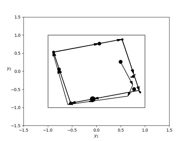
Figure 1. The state trajectory - 50 time steps.

Remark. Note that the control $u^{N}(y)$ defined as a minimizer in (46) is near optimal only in a neighbourhood of the optimal trajectory that starts at $y_{0}$. If, instead of $\psi^{N}(\cdot)$, an approximation of the optimal value function is used in the right-hand-side of (46), then the corresponding minimizer will be near optimal for all $y\in Y$. A most common approach to finding an approximation of the optimal value function is based on a discretization of the state space and solving the corresponding dynamic programming equation for thus obtained finite state space process (see, e.g., Appendix A in [4]). The finer is the grid of the discretization, the better are approximations of the optimal value and the optimal control. In contrast to this approach, the function $\psi^{N}(\cdot)$, being an approximate solution of the max-min problem (7), is obtained via solving the semi-infinite dimensional (SID) linear programming problem (49), and the proximity of an approximation depends on the number $N$ of the test functions in (50). While solving the SIDLP problem (49) requires a discretization of the state space, the grid of the discretization does not need to be fine. In fact, the algorithm proposed in [21] aims at finding the grid points (their number being no more than $N$) that are concentrated around the optimal trajectory. Arguably, this may require less computational efforts than the classic approach although, of course, more research is needed to validate this claim.

6. Generalization of Theorem 4.1 and a heuristic numerical algorithm

Finding a minimizer in (46) may be a challenging task since the problem in the right-hand-side of (46) is generally not of the convex programming class (even in the case when $g(y,u)$ is convex and $f(y,u)$ is linear in $u$). This difficulty can be avoided since the only property of the minimizer $u^{N}(y)$ that was used in proving that it is near optimal for large $N$ is that it satisfies the equalities

$$u^{N}(y^{N}_{j})=u^{N}_{j},\ \ j=1,...,K_{N},$$ (65)

where $(y^{N}_{j},u^{N}_{j})$ are the concentration points of the Dirac measures in the presentation (54) (see Proposition 7). Having this in mind, one can establish a more general result suggesting that a simpler way of constructing a near optimal control is possible. To state the result, let us introduce the following assumption.

ASSUMPTION II: Let the set of the concentration points $\{(y^{N}_{j},u^{N}_{j}),\ j=1,...,K_{N}\}$ does not contain points with the same $y$-coordinates and different $u$-coordinates.

Note that, under Assumption II (which is assumed to be valid everywhere in this section), one can define the function $\xi^{N}(\cdot)$,

$$\xi^{N}(y^{N}_{j}):=u^{N}_{j},\ \ j=1,...,K_{N}.$$ (66)

This function is defined on the set of $y$-coordinates of the concentration points $\{(y^{N}_{j},u^{N}_{j}),\ j=1,...,K_{N}\}$ and it takes values in the set of $u$-coordinates of these points.

We will call a function $u^{N}(\cdot)$ an extension of $\xi^{N}(\cdot)$ onto $Y$ if $u^{N}(y)\in A(y)\ \ \forall\ y\in Y$ and if the equalities (65) are satisfied. (As has been mentioned above, the minimizer in (46) is an example of such an extension.) The following theorem establishes that, under conditions similar to those of Theorem 4.1, an extension of $\xi^{N}(\cdot)$ onto $Y$ is near optimal for $N$ is large enough.

Theorem 6.1.

Let $u^{N}(\cdot)$ be an extension of $\xi^{N}(\cdot)$ onto $Y$ and let $y^{N}(\cdot)$ be the solution of (47) satisfying the initial condition $y^{N}(0)=y_{0}$. Let (43) be satisfied, the functions $f$ and $g$ be Lipschitz continuous and the optimal solution $\gamma^{*}$ of problem (11) be unique. Assume also that there exists an optimal admissible process $(\bar{y}(\cdot),\bar{u}(\cdot))$ such that:

(a) For any $t\in{\mathcal{T}}$ there exists an open ball $Q_{t}$ centered at $\bar{y}(t)$ such that $u^{N}(\cdot)$ is Lipschitz continuous on $Q_{t}$ with Lipschitz constant independent of $N$ and $t$;

(b) $y^{N}(t)\in Q_{t}\ \forall t\in{\mathcal{T}}$ for sufficiently large $N$.

Then the relationships (48) are valid.

Proof. The proof follows exactly the same steps as those in the proof of Theorem 4.1. $\Box$

In the case when the map $A(y)$ is constant-valued, it is natural do define an extension $u^{N}(\cdot)$ of $\xi^{N}(\cdot)$ in such way that it takes constant values on some neighbourhoods of the $y$-components of the concentration points $\ \{(y^{N}_{j},u^{N}_{j}),\ j=1,...,K_{N}\}$. That is, $\ u^{N}(y)=u^{N}_{j}$ for all $y$ in some “sufficiently small” neighborhood of $\ y^{N}_{j}$ for all $j=1,...,K_{N}$. (Note that, due to Proposition 8, one may expect that the optimal admissible trajectory $\bar{y}(\cdot)$ is contained in the union of these neighbourhoods if $N$ is large enough.)

Using the idea of such piecewise constant extension of $\xi^{N}(\cdot)$, one can propose the following heuristic algorithm for the construction of a control that can be a “good candidate” for being near optimal in (2):

Heuristic algorithm for the construction of a near optimal control.

1. Find an optimal solution of the semi-infinite LP problem (49). That is, find the concentration points $\ \{(y^{N}_{j},u^{N}_{j})\}$ of the Dirac measures and the weights $\{\beta^{N}_{j}\}$, $\ j=1,...,K_{N},$ in the presentation (54), and evaluate the optimal value $g_{N}^{*}(y_{0})$ of this problem.

2. Among the $y$-components of the concentration points, choose one which is closest to $y_{0}$. That is, choose $\ j_{0}:={\rm argmin}_{j}\{|y^{N}_{j}-y_{0}|\}$ and define

$$u^{N}(0):=u^{N}_{j_{0}},\ \ \ \ \ y^{N}(1):=f(y_{0},u^{N}(0)).$$

Assume that $u^{N}(0),...,u^{N}(t-1)$ and $y^{N}(1),...,y^{N}(t)$, where $t\geq 1$, have been defined. Then $u^{N}(t)$ and $y^{N}(t+1)$ are defined as follows:

$$u^{N}(t):=u^{N}_{j_{t}},\ \ \ \ \ y^{N}(t+1):=f(y^{N}(t),u^{N}(t)),$$

where $j_{t}:={\rm argmin}_{j}\{|y^{N}_{j}-y^{N}(t)|\}$.

3. Continue this process until the moment $t=T$ when the $\ \frac{\alpha^{T+1}}{1-\alpha}$ becomes small enough, making the finite sum $\sum_{t=0}^{T}\alpha^{t}g(y^{N}(t),u^{N}(t)):={V}^{N}(y_{0})$ a good approximation for the value of the objective function on the infinite time horizon. Evaluate the difference $\ |{V}^{N}(y_{0})-g_{N}^{*}(y_{0})(1-\alpha)^{-1}|$ that provides a measure of near optimality of the constructed control.

Remark. If for some $t\geq 0$ the minimizer in the problem $\ {\rm min}_{j}\{|y^{N}_{j}-y^{N}(t)|\}$ is not unique, then one can take $\ j_{t}:={\rm argmax}_{j\in J_{t}}\{\beta^{N}_{j}\}$, where $\ J_{t}:={\rm Argmin}_{j}\{|y^{N}_{j}-y^{N}(t)|\}$. That is, among the concentration points the $y$-components of which are equally close to $y^{N}(t)$, one can choose one that has the greatest weight. Note that a weight $\beta^{N}_{j}$ in the sum $\sum_{j=1}^{K_{N}}\beta_{j}^{N}\delta_{(y_{j}^{N},u_{j}^{N})}$ (see (54)) can be interpreted as an approximation of the number of times the optimal trajectory “attends” a vicinity of the corresponding $y^{N}_{j}$ (each subsequent attendance being time discounted).

Let us illustrate the way the algorithm outlined above works with the help of the example considered in Section 5.

Example 1 (continued). A sample of the concentration points $\ y_{j}^{N}=(y_{1,j}^{N},y_{2,j}^{N})$, $\ u_{j}^{N}=(u_{1,j}^{N},u_{2,j}^{N})$ of the Dirac measures entering (54) and the values of the corresponding weights $\{\beta^{N}_{j}\}$, $\ j=1,...,K_{N}$ is shown in the table below (these being a part of the solution of the SIDLP problem of Example 1).

$y_{1,j}^{N}$	$y_{2,j}^{N}$	$u_{1,j}^{N}$	$u_{2,j}^{N}$	$\beta_{j}^{N}$
-0.5375	-0.875	1	-1	0.0913
0.5	0.25	-1	1	0.0820
0.7625	-0.4875	1	1	0.0642
-0.775	0.05	1	-1	0.0538
0.8875	-0.5625	1	1	0.0536
-0.0875	-0.75	1	1	0.0525

(The concentration points with weights that are less than $10^{-2}$ were discarded, the number of terms in (54) after the discarding being equal to $27$.)

Among the concentration points shown in the table above, there is one with the $y$-coordinates $(0.5,0.25)$, these coinciding with the initial conditions (63). Thus, we take ${u}^{N}(0)$ to be equal to the corresponding $u$-coordinates of this point, ${u}^{N}(0)=(-1,1)$, which being substituted into the equations of the dynamics, leads to ${y}^{N}(1)=(0.75,-0.375)$. The closest to ${y}^{N}(1)$ (of all $y$ components of the concentration points) is the pair $(0.7625,-0.4875)$; the latter is marked by a dot in Fig. 2. The corresponding $u$-components of the concentration point are $(1,1)$. We, therefore, take ${u}^{N}(1)=(1,1)$ and obtain ${y}^{N}(2)=(-0.125,-0.6875)$. The closest to ${y}^{N}(2)$ are the $y$-coordinates $(-0.0875,-0.75)$ marked in Fig 3. The corresponding $u$-components of the concentration point are $(1,1)$, and, consequently, ${u}^{N}(2)=(1,1)$, etc.

This process has been repeated $50$ times and the resulted state trajectory is depicted in Fig. 4. Note that it looks similar to that depicted in Fig 1. The value of the objective function thus obtained was evaluated to be approximately equal to $-10.03$ (${V}^{N}(y_{0})\approx-1.003$). Finally, we obtain

$$|{V}^{N}(y_{0})-g_{N}^{*}(y_{0})(1-\alpha)^{-1}|\approx(-10.03)-(-10.13)=0.1,$$

the error being less than in the case when the control defined as a minimizer (46) was used.

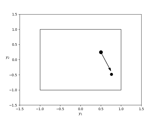
Figure 2.  The state trajectory - time step 1.

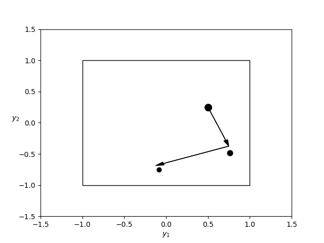
Figure 3. The state trajectory - time steps 1 and 2.

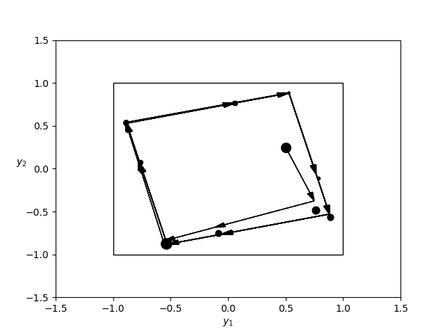
Figure 4. The state trajectory - 50 time steps.

Remark. As has been mentioned above, results obtained in this paper are in many ways analogous to similar results in continuous time setting obtained in [21]. Let us briefly outline relationships between these two sets of results. Firstly, all results of the present paper are established for the case when the control set may depend on the state variables, with the only restriction on this dependence being that the map $U(\cdot)$ is upper semicontinuous and compact valued. The consideration in [21] was for the fixed control set, that is without the dependence of the latter on the state variables. Moreover, allowing such dependence in the continuous time setting would make the consideration much more technical (requiring, e.g., additional regularity assumptions about the map $U(\cdot)$). Secondly, the $max$ in the max-min problem (7) is over the class of bounded lower semicontinuous functions, this being in contrast to the continuous time max-min counterpart of (7), in which $max$ (or rather $sup$) was over the set of smooth functions. While maximizer in (7) always exists, a maximizer in the continuous counterpart of (7) may not exist and its existence needs to be assumed, this being a restrictive assumption (compare Theorem 2.1 and Proposition 2.1 in [21]).

As far as the algorithmic part of the paper is concerned, finding a minimizer in problem (46) is generally a more difficult task than finding a minimizer in the continuous time counterpart of (46) (see Section 3 in [21]). For example, the latter is of convex programming while the former is generally not in case $g(y,u)$ is convex and $f(y,u)$ is linear in $u$. In Section 6, we proposed a way allowing one to avoid solving (46), this being also possible in continuous time setting (such an opportunity was not investigated in [21]).

References

[1] (MR2125136) [10.1287/moor.1040.0109]
D. Adelman and D. Klabjan,
\doititleDuality and existence of optimal policies in generalized joint replenishment,
Mathematics of Operations Research, 30 (2005), 28–50.
[2] (MR0435321)
R. Ash,
Measure, Integration and Functional Analysis,
Academic Press, 1972.
[4] (MR1484411) [10.1007/978-0-8176-4755-1]
M. Bardi and I. Capuzzo-Dolcetta,
Optimal Control and Viscosity Solutions of Hamilton-Jacobi-Bellman Equations, Systems and Control: Foundations and Applications,Birkhäuser, Boston, 1997.
[5] (MR3644954)
D. Bertsekas,
Dynamic Programming and Optimal Control,Athena Scientific, Belmont, MA, 2017.
[6] (MR1411505) [10.1214/aop/1065725192]
A. G. Bhatt and V. S. Borkar,
\doititleOccupation measures for controlled Markov processes: Characterization and optimality,
Annals of Probability, 24 (1996), 1531–1562.
[7]
P. Billingsley,
Convergence of Probability Measures, John Wiley & Sons, New York, 1968.
[8] (MR2918256)
J. Blot,
A Pontryagin principle for infinite-horizon problems under constraints,
Dynamics of Continuous, Discrete and Impulsive Systems Series B: Applications and Algorithms, 19 (2012), 267–275.
[9] (MR0950347) [10.1007/BF00353877]
V. S. Borkar,
\doititleA convex analytic approach to Markov decision processes,
Probability Theory and Related Fields,78 (1988), 583–602.
[10] (MR2772196) [10.1007/s00245-010-9120-y]
R. Buckdahn, D. Goreac and M. Quincampoix,
\doititleStochastic optimal control and linear programming approach,
Appl. Math. Optim.63 (2011), 257–276.
[11] (MR3155340) [10.1007/978-3-642-76755-5]
D. A. Carlson, A. B. Haurier and A. Leizarowicz,
Infinite Horizon Optimal Control. Deterministic and Stochastic Processes,
Springer, Berlin, 1991.
[12] (MR1009162)
N. Dunford and J. T. Schwartz,
Linear Operators, Part I, General Theory,
Wiley & Sons, Inc., New York, 1988.
[13] (MR2421325) [10.1137/060676398]
L. Finlay, V. Gaitsgory and I. Lebedev,
\doititleDuality in linear programming problems related to deterministic long run average problems of optimal control,
SIAM J. Control and Optimization, 47 (2008), 1667–1700.
[14] (MR1009341) [10.1137/0327060]
W. H. Fleming and D. Vermes,
\doititleConvex duality approach to the optimal control of diffusions,
SIAM J. Control Optimization, 27 (1989), 1136–1155.
[15] (MR2082704) [10.1137/S0363012903424186]
V. Gaitsgory,
\doititleOn representation of the limit occupational measures set of control systems with applications to singularly perturbed control systems,
SIAM J. Control and Optimization, 43 (2004), 325–340.
[16] [0.1109/CDC.2016.7798950]
V. Gaitsgory, A. Parkinson and I. Shvartsman,
\doititleLinear programming formulation of a discrete time infinite horizon optimal control problem with time discounting criterion,
Proceedings of 55th IEEE Conference on Decision and Control (CDC), 2016, Las Vegas, USA.
[17] (MR3693843)
V. Gaitsgory, A. Parkinson and I. Shvartsman,
\doititleLinear Programming Formulations of Deterministic Infinite Horizon Optimal Control Problems in Discrete Time,
Discrete and Continuous Dynamical Systems, Series B, 22(10) (2017), 3821–3838.
[18] (MR2556353) [10.1137/070696209]
V. Gaitsgory and M. Quincampoix,
\doititleLinear programming approach to deterministic infinite horizon optimal control problems with discounting,
SIAM J. Control and Optim., 48 (2009), 2480–2512.
[19] (MR3057046) [10.1016/j.na.2013.03.015]
V. Gaitsgory and M. Quincampoix,
\doititleOn sets of occupational measures generated by a deterministic control system on an infinite time horizon,
Nonlinear Analysis (Theory, Methods & Applications), 88 (2013), 27–41.
[20] (MR2248173) [10.1137/040616802]
V. Gaitsgory and S. Rossomakhine,
\doititleLinear programming approach to deterministic long run average problems of optimal control,
SIAM J. of Control and Optimization, 44 (2006), 2006–2037.
[21] (MR2918249)
V. Gaitsgory, S. Rossomakhine and N. Thatcher,
\doititleApproximate solution of the HJB inequality related to the infinite horizon optimal control problem with discounting,
Dynamics of Continuous, Discrete and Impulsive Systems
Series B: Applications and Algorithms, 19 (2012), 65–92.
[22] (MR3041666) [10.1051/cocv/2011183]
D. Goreac and O.-S. Serea,
\doititleLinearization techniques for - control problems and dynamic programming principles in classical and control problems,
ESAIM: Control, Optimization and Calculus of Variations, 18 (2012), 836–855.
[23] (MR1626864) [10.1137/S0363012997315919]
L. Grüne,
\doititleAsymptotic controllability and exponential stabilization of nonlinear control systems at singular points,
SIAM J. Control Optim., 36 (1998), 1495–1503.
[24] (MR1637521) [10.1006/jdeq.1998.3451]
L. Grüne,
\doititleOn the relation between discounted and average optimal value functions,
J. Diff. Equations, 148 (1998), 65–69.
[25] (MR1404981)
D. Hernandez-Hernandez, O. Hernandez-Lerma and M. Taksar,