Improved Lower Bounds for the Fourier Entropy/Influence Conjecture via Lexicographic Functions

Abstract

Every Boolean function can be uniquely represented as a multilinear polynomial. The entropy and the total influence are two ways to measure the concentration of its Fourier coefficients, namely the monomial coefficients in this representation: the entropy roughly measures their spread, while the total influence measures their average level. The Fourier Entropy/Influence conjecture of Friedgut and Kalai from 1996 states that the entropy to influence ratio is bounded by a universal constant $C$.

Using lexicographic Boolean functions, we present three explicit asymptotic constructions that improve upon the previously best known lower bound $C>6.278944$ by O’Donnell and Tan, obtained via recursive composition. The first uses their construction with the lexicographic function $\ell\left\langle 2/3\right\rangle$ of measure $2/3$ to demonstrate that $C\geq 4+3\log_{4}3>6.377444$. The second generalizes their construction to biased functions and obtains $C>6.413846$ using $\ell\left\langle\Phi\right\rangle$, where $\Phi$ is the inverse golden ratio. The third, independent, construction gives $C>6.454784$, even for monotone functions.

Beyond modest improvements to the value of $C$, our constructions shed some new light on the properties sought in potential counterexamples to the conjecture.

Additionally, we prove a Lipschitz-type condition on the total influence and spectral entropy, which may be of independent interest.

1 Introduction

Let ${\bf true}=-1$ and ${\bf false}=+1$. Throughout this paper, we write $\left[n\right]=\left\{1,2,\ldots,n\right\}$ and $N=2^{n}$ for an integer $n\geq 1$. It is well known that any function $f:\left\{{\bf true},{\bf false}\right\}^{n}\to\mathbb{R}$ can be expressed as

$$f=\sum_{S\subseteq\left[n\right]}\hat{f}\left(S\right)\chi_{S},$$

where $\chi_{S}\left(x\right)=\prod_{i\in S}x_{i}$ for $S\subseteq\left[n\right]$ are the Fourier basis functions and

$$\hat{f}\left(S\right)=\left\langle f,\chi_{S}\right\rangle={\rm\mathbf{E}}\left[f\left(x\right)\chi_{S}\left(x\right)\right]$$

for $S\subseteq\left[n\right]$ are called the Fourier coefficients of $f$. When $f$ is a Boolean function, i.e., $f:\left\{{\bf true},{\bf false}\right\}^{n}\to\left\{{\bf true},{\bf false}\right\}$, we have $\sum_{S\subseteq\left[n\right]}\hat{f}\left(S\right)^{2}=1$ by Parseval, so we can treat the Fourier coefficients’ squares as a probability distribution $p_{f}$ on the $N$ subsets of $\left[n\right]$, which we call the spectral distribution of $f$.

The following two parameters of the function $f$ can be defined in terms of its spectral distribution.

Definition.

The total influence (also called average sensitivity) of a Boolean function $f$ is

$${\bf I}\left[f\right]={\rm\mathbf{E}}_{S\sim p_{f}}\left[\left|S\right|\right].$$

Definition.

The spectral entropy of a Boolean function $f$ is the (Shannon) entropy of its spectral distribution

$${\bf H}\left[f\right]={\rm\mathbf{E}}_{S\sim p_{f}}\left[-\log_{2}\left(p_{f}\left(S\right)\right)\right]=-\sum_{S}p_{f}\left(S\right)\log_{2}\left(p_{f}\left(S\right)\right).$$

In 1996 Friedgut and Kalai raised the following conjecture, known as the Fourier Entropy/Influence (FEI) conjecture:

Conjecture 1.1 ([4]).

There exists a universal constant $C>0$ such that for every Boolean function $f$ with total influence ${\bf I}\left[f\right]$ and spectral entropy ${\bf H}\left[f\right]$ we have ${\bf H}\left[f\right]\leq C\cdot{\bf I}\left[f\right]$.

Conjecture 1.1 was verified for various families of Boolean functions (e.g., symmetric functions [10], random functions [3], read-once formulas [1, 9], decision trees of constant average depth [11], read-$k$ decision trees for constant $k$ [11]) but is still open for the class of general Boolean functions.

The rest of this paper is organized as follows. In the remainder of Section 1 we describe past results and some rudimentary improvements. In Section 2 we introduce lexicographic functions and provide a formal proof of the approach described in Section 1.3. In Section 3 we generalize Proposition 1.2 to biased functions and get an improved lower bound. In Section 4 we build a limit-of-limits function that achieves an even better bound. In Section 5 we prove a Lipschitz-type condition used throughout the paper, namely that a small change in a Boolean function cannot result in a substantial change to its total influence and spectral entropy.

1.1 A baby example and two definitions

Here is a example of providing a lower bound on C. For $n\geq 1$ consider the function

$${\rm And}_{n}\left(x_{1},\ldots,x_{n}\right)=x_{1}\wedge x_{2}\wedge\cdots\wedge x_{n}.$$

It satisfies ${\bf I}\left[{\rm And}_{n}\right]=2n/N$ and ${\bf H}\left[{\rm And}_{n}\right]\approx 8\left(n-1+1/\ln 4\right)/N,$ so any constant $C$ in Conjecture 1.1 must satisfy

$$C\geq{\bf H}\left[{\rm And}_{n}\right]/{\bf I}\left[{\rm And}_{n}\right]\approx 4-\frac{4}{n}\left(1-1/\ln 4\right).$$

This is true for every $n$, so by taking $n\to\infty$ we establish that $C\geq 4$.

Definition.

A Boolean function $f$ is called monotone if changing an input bit $x_{i}$ from ${\bf false}$ to ${\bf true}$ cannot change the output $f\left(x\right)$ from ${\bf true}$ to ${\bf false}$.

Fact.

A Boolean function is monotone if and only if it can be expressed as a formula combining variables using conjunctions ($\wedge$) and disjunctions ($\vee$) only, with no negations.

Definition.

Let $f$ be a Boolean function on $n$ variables. The dual function of $f$, denoted $f^{\dagger}$, is defined as

$$f^{\dagger}\left(x_{1},\ldots,x_{n}\right)=\neg f\left(\neg x_{1},\ldots\neg x_{n}\right).$$

Fact.

For all $S\subseteq\left[n\right]$ we have $\hat{f^{\dagger}}\left(S\right)=\left(-1\right)^{\left|S\right|+1}\hat{f}\left(S\right)$.

Corollary.

The spectral distributions $p_{f}$ and $p_{f^{\dagger}}$ are identical; in particular, ${\bf I}\left[f^{\dagger}\right]={\bf I}\left[f\right]$ and ${\bf H}\left[f^{\dagger}\right]={\bf H}\left[f\right]$. But ${\rm\mathbf{E}}\left[f^{\dagger}\right]=-{\rm\mathbf{E}}\left[f\right]$ and ${\rm Pr}\left[f^{\dagger}\left(x\right)={\bf true}\right]=1-{\rm Pr}\left[f\left(x\right)={\bf true}\right]$.

Remark.

If $f$ is monotone then $f^{\dagger}$ is monotone too. Furthermore, given a monotone formula computing $f$, the formula obtained by swapping conjunctions and disjunctions computes $f^{\dagger}$.

Example.

The dual of ${\rm Or}_{n}\left(x_{1},\ldots,x_{n}\right)=x_{1}\vee x_{2}\vee\cdots\vee x_{n}$ is ${\rm And}_{n}$.

1.2 Past results and preliminary improvements

The current best lower bound on $C$ was achieved by O’Donnell and Tan [9]. Using recursive composition they showed the following bound:

Proposition 1.2.

Let $g$ be a balanced Boolean function such that ${\bf H}\left[g\right]>0$. Then any constant $C$ in Conjecture 1.1 satisfies $C\geq{\bf H}\left[g\right]/\left({\bf I}\left[g\right]-1\right).$

Remark.

Any balanced Boolean function $g$ has ${\bf I}\left[g\right]\geq 1$ since $p_{g}\left(\varnothing\right)={\rm\mathbf{E}}\left[g\right]=0$; in case of equality we must have $g=\chi_{\left\{i\right\}}$ for some $i\in\left[n\right]$ and thus $p_{g}$ is supported on a single set $S=\left\{i\right\}$ and its spectral entropy is zero.

By presenting a function on $6$ variables with total influence $I=13/8=1.625$ and entropy $H>3.92434$, they established that $C>3.92434/\frac{5}{8}=6.278944$. Although the specific function presented in [9] happens to be biased, their result stands as there exists a balanced Boolean function $g_{3}$ on 6 variables with the same total influence and entropy:

$$g_{3}\left(x_{1},x_{2},x_{3},x_{4},x_{5},x_{6}\right)=\left(x_{1}\vee x_{2}\right)\wedge\left(x_{3}\vee x_{4}\right)\wedge\left(x_{1}\vee x_{3}\vee x_{5}\right)\wedge\left(x_{3}\vee x_{5}\vee x_{6}\right).$$

A slight improvement can be achieved by modifying the last clause of $g_{3}$. Indeed,

$$g_{3}^{\prime}\left(x_{1},x_{2},x_{3},x_{4},x_{5},x_{6}\right)=\left(x_{1}\vee x_{2}\right)\wedge\left(x_{3}\vee x_{4}\right)\wedge\left(x_{1}\vee x_{3}\vee x_{5}\right)\wedge\left(x_{2}\vee x_{4}\vee x_{6}\right)$$

is balanced too, with the same total influence ${\bf I}\left[g_{3}^{\prime}\right]={\bf I}\left[g_{3}\right]=13/8$ and a slightly higher entropy ${\bf H}\left[g_{3}^{\prime}\right]>3.9669$, so we have $C>3.9669/\frac{5}{8}=6.34704$.

Moving to balanced functions on 8 variables, we find a monotone function $g_{4}$ that provides a better lower bound:

$$g_{4}\left(x_{1},\ldots,x_{8}\right)=\left(x_{1}\vee x_{2}\right)\wedge\left(x_{3}\vee x_{4}\right)\wedge\left(x_{3}\vee x_{5}\vee x_{6}\right)\wedge\left(x_{1}\vee x_{3}\vee x_{5}\vee x_{7}\right)\wedge\left(x_{3}\vee x_{5}\vee x_{7}\vee x_{8}\right)$$

with ${\bf I}\left[g_{4}\right]=53/32$ and ${\bf H}\left[g_{4}\right]>4.16885$ yields $C>6.35253$.

A further search discovers a slightly superior function:

$$g_{4}^{\prime}\left(x_{1},\ldots,x_{8}\right)=\left(x_{1}\vee x_{2}\right)\wedge\left(x_{3}\vee x_{4}\right)\wedge\left(x_{3}\vee x_{5}\vee x_{6}\right)\wedge\left(x_{1}\vee x_{3}\vee x_{5}\vee x_{7}\right)\wedge\left(x_{2}\vee x_{3}\vee x_{6}\vee x_{8}\right)$$

with ${\bf I}\left[g_{4}^{\prime}\right]={\bf I}\left[g_{4}\right]=53/32$ and ${\bf H}\left[g_{4}^{\prime}\right]>4.17635$ achieves $C>6.36396$.

1.3 Sequences of balanced monotone functions

Staring at $g_{3}$, $g_{4}$ and $g_{4}^{\prime}$ for a moment (but not $g_{3}^{\prime}$), we may see a common property: $x_{3}$ appears in all clauses except the first. Let us rewrite $g_{3}$ and $g_{4}$ in a slightly different form:

$$g_{3}\left(x_{1},\ldots,x_{6}\right) = \left(x_{1}\vee x_{2}\right)\wedge\left(x_{3}\vee\left(x_{4}\wedge\left(x_{5}\vee\left(x_{6}\wedge x_{1}\right)\right)\right)\right),$$

$$g_{4}\left(x_{1},\ldots,x_{8}\right) = \left(x_{1}\vee x_{2}\right)\wedge\left(x_{3}\vee\left(x_{4}\wedge\left(x_{5}\vee\left(x_{6}\wedge\left(x_{7}\vee\left(x_{8}\wedge x_{1}\right)\right)\right)\right)\right)\right).$$

This generalizes easily to a sequence $\left(g_{m}\right)_{m\geq 1}$ of balanced (to be shown below) monotone Boolean functions:

$$g_{m}\left(x_{1},\ldots,x_{2m}\right)=\left(x_{1}\vee x_{2}\right)\wedge\left(x_{3}\vee\left(x_{4}\wedge\left(x_{5}\vee\cdots\left(x_{2m-1}\vee\left(x_{2m}\wedge x_{1}\right)\right)\cdots\right)\right)\right)$$

whose first two members are

$$g_{1}\left(x_{1},x_{2}\right) = \left(x_{1}\vee x_{2}\right)\wedge x_{1}=x_{1},$$

$$g_{2}\left(x_{1},x_{2},x_{3},x_{4}\right) = \left(x_{1}\vee x_{2}\right)\wedge\left(x_{3}\vee\left(x_{4}\wedge x_{1}\right)\right)=\left(x_{1}\vee x_{2}\right)\wedge\left(x_{3}\vee x_{4}\right)\wedge\left(x_{1}\vee x_{3}\right).$$

Denote by $C_{m}={\bf H}\left[g_{m}\right]/\left({\bf I}\left[g_{m}\right]-1\right)$ the lower bound on $C$ implied by $g_{m}$. The first fifteen members of the sequence are explored in Table 1. Note how even $C_{2}=6$ is much better than the $C\geq 4$ bound of Subsection 1.1.

$m$	$n$	${\bf I}\left[g_{m}\right]$	${\bf H}\left[g_{m}\right]$	$C_{m}$
1	2	1	0	(not defined)
2	4	$3/2=1.5$	3	6
3	6	$13/8=1.625$	$>3.92434$	$>6.27894$
4	8	$53/32=1.65625$	$>4.16885$	$>6.35253$
5	10	$213/128=1.6640625$	$>4.23087$	$>6.37119$
6	12	$853/512=\left(5-2^{-9}\right)/3$	$>4.24643$	$>6.37588$
7	14	$3413/2048=\left(5-2^{-11}\right)/3$	$>4.25033$	$>6.37705$
8	16	$13653/2^{13}=\left(5-2^{-13}\right)/3$	$>4.25130$	$>6.37734$
9	18	$54613/2^{15}=\left(5-2^{-15}\right)/3$	$>4.25154$	$>6.37741$
10	20	$\left(5-2^{-17}\right)/3$	$>4.251608$	$>6.377437$
11	22	$\left(5-2^{-19}\right)/3$	$>4.251624$	$>6.3774422$
12	24	$\left(5-2^{-21}\right)/3$	$>4.2516278$	$>6.3774433$
13	26	$\left(5-2^{-23}\right)/3$	$>4.25162885$	$>6.37744365$
14	28	$\left(5-2^{-25}\right)/3$	$>4.25162908$	$>6.37744372$
15	30	$\left(5-2^{-27}\right)/3$	$>4.251629147$	$>6.377443745$

Table 1: Parameters of the sequence $g_{m}$ for $m\leq 15$

The three sequences seem to be increasing and bounded, so let us denote their respective hypothetical limits by $I_{*}$, $H_{*}$ and $C_{*}$. If indeed ${\bf I}\left[g_{m}\right]=\frac{1}{3}\left(5-2^{3-2m}\right)$ for all $m\in\mathbb{N}$ then $I_{*}=5/3$. A prescient guess for the value of $H_{*}$ could be

$$H_{*}=\frac{8}{3}+\log_{2}3>4.251629167,$$

for which we would get

$$C_{*}=H_{*}/\left(2/3\right)=4+3\log_{4}3>6.377443751$$

as a lower bound for $C$. We will verify this guess in Section 2.

Recall that $g_{3}^{\prime}$ and $g_{4}^{\prime}$ gave rise to better lower bounds, respectively, than $g_{3}$ and $g_{4}$. It is tempting perhaps to consider a generalization $\left(g_{m}^{\prime}\right)_{m\geq 3}$, define $C_{m}^{\prime}$ accordingly and examine the hypothetical limits $I_{*}^{\prime}$, $H_{*}^{\prime}$ and $C_{*}^{\prime}$. It is indeed possible to do so, and we get ${\bf I}\left[g_{m}^{\prime}\right]={\bf I}\left[g_{m}^{\prime}\right]$ while ${\bf H}\left[g_{m}^{\prime}\right]>{\bf H}\left[g_{m}\right]$, making $C^{\prime}_{m}>C_{m}$. Nevertheless, ${\bf H}\left[g_{m}^{\prime}\right]$ and $C^{\prime}_{m}$ seem to converge towards the same $H_{*}$ and $C_{*}$, respectively, so there is no real benefit in pursuing this further.

It remains to verify that $g_{m}$ is indeed balanced for all $m\geq 1$. Let us write it as

$$g_{m}\left(x_{1},\ldots,x_{2m}\right)=\left(x_{1}\vee x_{2}\right)\wedge G_{m}\left(x_{3},x_{4},\ldots,x_{2m},x_{1}\right),$$

where $G_{m}\left(y_{1},y_{2},\ldots,y_{2m-1}\right)$ is defined recursively via

$$G_{1}\left(y_{1}\right) = y_{1},$$

$$G_{m+1}\left(y_{1},\ldots,y_{2m+1}\right) = y_{1}\vee\left(y_{2}\wedge G_{m}\left(y_{3},\ldots,y_{2m+1}\right)\right).$$

Remark.

The function $G_{m}$ belongs to a class of monotone Boolean functions called lexicographic functions, as we will see in Section 2.1.

For simplicity of notation, we abbreviate and write ${\rm Pr}\left[f\left(x\right)\right]$ or even ${\rm Pr}\left[f\right]$ to denote ${\rm Pr}\left[f\left(x\right)={\bf true}\right]$. Since

$${\rm Pr}\left[g_{m}\left(x\right)\right]={\rm Pr}\left[x_{1}\vee x_{2}\right]\cdot{\rm Pr}\left[G_{m}\left(x_{3},\ldots,x_{2m},x_{1}\right)\mid x_{1}\vee x_{2}\right],$$

to prove ${\rm Pr}\left[g_{m}\right]=\frac{1}{2}$, it suffices to verify the following (see Appendix A for the calculation):

Claim 1.3.

For all $m\geq 1$ we have ${\rm Pr}\left[G_{m}\left(x_{3},\ldots,x_{2m},x_{1}\right)\mid x_{1}\vee x_{2}\right]=2/3$.

2 A Tale of Two Thirds

Although each of $\left(C_{m}\right)_{m=2}^{15}$ from Table 1 is a valid, explicit lower bound on $C$, the asymptotic discussion in Subsection 1.3 was more of a wishful thinking rather than a mathematically sound statement.

In this section we explore the class of lexicographic functions, develop tools to compute total influence and spectral entropy, and then rigorously calculate $I_{*}$, $H_{*}$ and $C_{*}$.

2.1 Lexicographic functions

Definition.

Fix integers $n\geq 1$ and $0\leq s\leq N$. Denote by $L_{n}\left\langle s\right\rangle\subseteq\left\{{\bf true},{\bf false}\right\}^{n}$ the initial segment of cardinality $s$ (with respect to the lexicographic order on $\left\{{\bf true},{\bf false}\right\}^{n}$), and denote by $\ell_{n}\left\langle s\right\rangle:\left\{{\bf true},{\bf false}\right\}^{n}\to\left\{{\bf true},{\bf false}\right\}$ its characteristic function

$$\ell_{n}\left\langle s\right\rangle\left(x\right)=\begin{cases}{\bf true},&x\in L_{n}\left\langle s\right\rangle;\\ {\bf false},&x\not\in L_{n}\left\langle s\right\rangle.\end{cases}$$

Fact.

We have ${\rm Pr}\left[\ell_{n}\left\langle s\right\rangle\right]=\left|L_{n}\left\langle s\right\rangle\right|/N=s/N$ and ${\rm\mathbf{E}}\left[\ell_{n}\left\langle s\right\rangle\right]=1-2s/N$.

Fact.

The function $\ell_{n}\left\langle s\right\rangle$ is monotone and its dual is $\left(\ell_{n}\left\langle s\right\rangle\right)^{\dagger}=\ell_{n}\left\langle N-s\right\rangle$.

Example.

$\ell_{n}\left\langle 1\right\rangle={\rm And}_{n}$ and $\ell_{n}\left\langle N-1\right\rangle={\rm Or}_{n}$.

Fact.

If $s$ is even then $\ell_{n}\left\langle s\right\rangle$ is isomorphic to $\ell_{n-1}\left\langle s/2\right\rangle$ (when the latter is extended from $n-1$ to $n$ variables by adding an influenceless variable).

Let $0<s<N$ be an odd integer, and let $s_{1}s_{2}\cdots s_{n}$ be its binary representation, where $s_{1}$ is the most significant bit and $s_{n}=1$ is the least significant bit. Denote the corresponding $\left\{{\bf true},{\bf false}\right\}^{n}$ representation of $s$ by $\vec{s}=\left(\left(-1\right)^{s_{1}},\ldots,\left(-1\right)^{s_{n}}\right)$.

By definition, to determine the value of $\ell_{n}\left\langle s\right\rangle$ for an input $x$, we need to compare $x$ with $\vec{s}$ element by element. This gives a neat formula for $\ell_{n}\left\langle s\right\rangle$:

$$\ell_{n}\left\langle s\right\rangle\left(x_{1},\ldots,x_{n}\right)=x_{1}\diamond_{1}\left(x_{2}\diamond_{2}\left(x_{3}\diamond_{3}\cdots\left(x_{n-1}\diamond_{n-1}x_{n}\right)\cdots\right)\right),$$ (1)

where $\diamond_{i}=\begin{cases}\wedge,&s_{i}=0;\\ \vee,&s_{i}=1.\end{cases}$

Remark.

The formula (1) shows that every monotone decision list, i.e., a monotone decision tree consisting of a single path, is isomorphic to a lexicographic function.

From (1) we derive an important property of lexicographic functions.

Fact 2.1.

For $k\in\left[n\right]$, the value of $\ell_{n}\left\langle s\right\rangle$$\left(x\right)$ only depends on $x_{k}$ with probability $2^{1-k}$; that is, when $x_{i}=\left(-1\right)^{s_{i}}$ for all $i<k$.

Remark.

This can be interpreted as saying that the average decision tree complexity of $\ell_{n}\left\langle s\right\rangle$ is $2-\left(n+2\right)/N$.

We extend the definition of lexicographic functions by writing $\ell_{n}\left\langle\mu\right\rangle=\ell_{n}\left\langle\left\lfloor\mu N\right\rfloor\right\rangle$ for some $0\leq\mu\leq 1$. Note that $\left\lfloor\mu N\right\rfloor$ is not necessarily odd, so the effective number of variables can be smaller.

Example.

For any $n\geq 2$ we have $\ell_{n}\left\langle 3/4\right\rangle\left(x\right)=x_{1}\vee x_{2}$; that is, $\ell_{n}\left\langle 3/4\right\rangle={\rm Or}_{2}$.

Example.

For $n=2m-1$, we have $\ell_{n}\left\langle 2/3\right\rangle=\ell_{n}\left\langle\left\lfloor 2N/3\right\rfloor\right\rangle=\ell_{n}\left\langle\left(2N-1\right)/3\right\rangle$. Observe that the binary representation of the odd integer $s=\left(2N-1\right)/3$ has $s_{i}=i\bmod 2$ for $i\in\left[n\right]$ and thus

$$\ell_{n}\left\langle 2/3\right\rangle\left(x\right)=x_{1}\vee\left(x_{2}\wedge\left(x_{3}\vee\left(x_{4}\wedge\cdots\left(x_{2m-2}\wedge x_{2m-1}\right)\cdots\right)\right)\right),$$

that is, $\ell_{n}\left\langle 2/3\right\rangle=G_{m}$.

Fix $0<\mu<1$ and consider the sequence $\left(\ell_{n}\left\langle\mu\right\rangle\right)_{n\geq 1}$. Whenever $\mu$ is a dyadic rational, $\ell_{n}\left\langle\mu\right\rangle$ converges to a fixed function $\ell\left\langle\mu\right\rangle$ (e.g., $\ell\left\langle 3/4\right\rangle={\rm Or}_{2}$ in the example above). We would like to consider the limit object $\ell\left\langle\mu\right\rangle=\lim_{n}\ell_{n}\left\langle\mu\right\rangle$ for other values of $\mu$ as well.

It may sound intimidating; after all, $\ell\left\langle\mu\right\rangle:\left\{{\bf true},{\bf false}\right\}^{\mathbb{N}}\to\left\{{\bf true},{\bf false}\right\}$ is a Boolean function on $\aleph_{0}$ variables, which is quite a lot. Nevertheless, by Fact 2.1, $\ell\left\langle\mu\right\rangle$ only reads two input bits on average.

Moreover, we care about the total influence and spectral entropy of functions. By Lemmata 5.1 and 5.2 from Section 5, ${\bf I}\left[\ell_{n}\left\langle\mu\right\rangle\right]\xrightarrow{n\to\infty}{\bf I}\left[\ell\left\langle\mu\right\rangle\right]$ and ${\bf H}\left[\ell_{n}\left\langle\mu\right\rangle\right]\xrightarrow{n\to\infty}{\bf H}\left[\ell\left\langle\mu\right\rangle\right]$. Indeed, $\ell_{n}\left\langle\mu\right\rangle$ differs from $\ell_{n-1}\left\langle\mu\right\rangle$ (when considering the latter as a function on $n$ variables by adding an influenceless variable) in at most one place, and thus $\left({\bf I}\left[\ell_{n}\left\langle\mu\right\rangle\right]\right)_{n\geq 1}$ and $\left({\bf H}\left[\ell_{n}\left\langle\mu\right\rangle\right]\right)_{n\geq 1}$ are Cauchy sequences.

Needless to say, ${\rm Pr}\left[\ell_{n}\left\langle\mu\right\rangle\right]=\left\lfloor\mu N\right\rfloor/N\xrightarrow{n\to\infty}\mu={\rm Pr}\left[\ell\left\langle\mu\right\rangle\right]$.

An even stronger statement holds (but will not be used or proved here): the spectral distributions of $\ell_{n}\left\langle\mu\right\rangle$ converge in distribution to a limit distribution $p_{\mu}$, which we call the spectral distribution of $\ell\left\langle\mu\right\rangle$. Note that $p_{\mu}$ is supported on finite subsets of $\mathbb{N}$. The expected cardinality and the entropy of $S\sim p_{\mu}$ are ${\bf I}\left[\ell\left\langle\mu\right\rangle\right]$ and ${\bf H}\left[\ell\left\langle\mu\right\rangle\right]$ respectively.

2.2 Total influence and lexicographic functions

The edge isoperimetric inequality in the discrete cube (by Harper [5], with an addendum by Bernstein [2], and independently Lindsey [7]) gives a lower bound on the total influence of Boolean functions.

Theorem 2.2.

Let $f$ be a Boolean function with ${\rm Pr}\left[f\right]=\mu\leq\frac{1}{2}$. Then ${\bf I}\left[f\right]\geq-2\mu\log_{2}\mu$.

In fact, they proved that lexicographic functions are the minimizers of total influence.

Theorem 2.3.

Fix integers $n\geq 1$ and $s\leq N/2$ and let $f$ be a Boolean function on $n$ variables with ${\rm Pr}\left[f\right]=s/N$. Then ${\bf I}\left[f\right]\geq{\bf I}\left[\ell_{n}\left\langle s\right\rangle\right]$.

Remark.

Theorem 2.3 explains our interest in lexicographic functions: when seeking a function $f$ with large entropy/influence ratio ${\bf H}\left[f\right]/{\bf I}\left[f\right]$, it makes sense to minimize ${\bf I}\left[f\right]$.

In [6], Hart exactly computed the total influence of lexicographic functions:

Proposition 2.4 ([6, Theorem 1.5]).

Fix integers $n\geq 1$ and $0\leq s\leq N$. Then

$${\bf I}\left[\ell_{n}\left\langle s\right\rangle\right]=\frac{2sn}{N}-\frac{4}{N}\sum_{x=0}^{s-1}wt\left(x\right),$$

where $wt\left(x\right)$ is the Hamming weight of $x$.

Let us rephrase Proposition 2.4 a bit.

Claim 2.5.

Let $s=\sum_{i=0}^{t}N/2^{k_{i}}$, where $1\leq k_{0}<k_{1}<\cdots<k_{t}$ are the locations of $1$ in the binary representation of $s$. Then ${\bf I}\left[\ell_{n}\left\langle s\right\rangle\right]=\sum_{i=0}^{t}\left(k_{i}-2i\right)2^{1-k_{i}}$.

Proof.

By induction on $t$. For details see Appendix A. ∎

Example.

For $s=N/2^{k}$ we get ${\bf I}\left[{\rm And}_{k}\right]={\bf I}\left[\ell_{n}\left\langle N/2^{k}\right\rangle\right]=k2^{1-k}$, demonstrating the tightness of Theorem 2.2.

Corollary 2.6.

Let $\mu=\sum_{i=0}^{\infty}2^{-k_{i}}$, where $1\leq k_{0}<k_{1}<\cdots$ are the locations of $1$ in the binary representation of $\mu$. Then ${\bf I}\left[\ell\left\langle\mu\right\rangle\right]=\sum_{i=0}^{\infty}\left(k_{i}-2i\right)2^{1-k_{i}}$.

This leads to the following observation:

Fact.

For any $0\leq\mu\leq 1$ we have

$${\bf I}\left[\ell\left\langle\frac{1}{2}\pm\frac{\mu}{4}\right\rangle\right]=2\cdot 2^{-1}+\sum_{i=1}^{\infty}\left(\left(k_{i-1}+2\right)-2i\right)2^{1-\left(k_{i-1}+2\right)}=1+\frac{1}{4}{\bf I}\left[\ell\left\langle\mu\right\rangle\right].$$ (2)

Example.

For $\mu=\frac{2}{3}$ we have

$${\bf I}\left[\ell\left\langle 2/3\right\rangle\right]={\bf I}\left[\ell\left\langle 1/2+1/6\right\rangle\right]=1+\frac{1}{4}{\bf I}\left[\ell\left\langle 2/3\right\rangle\right],$$

hence ${\bf I}\left[\ell\left\langle 2/3\right\rangle\right]=\frac{4}{3}$. By duality we have ${\bf I}\left[\ell\left\langle 1/3\right\rangle\right]=\frac{4}{3}$ as well.

Remark.

Compare the bound $\frac{2}{3}\log_{2}3\approx 1.05664$ obtained for $\mu=\frac{1}{3}$ from Theorem 2.2 to ${\bf I}\left[\ell\left\langle 1/3\right\rangle\right]=4/3\approx 1.3333$ computed above. In fact, Theorem 2.2 is only tight when $\mu$ is a power of two.

Four-thirds is actually the maximum influence attainable by any lexicographic function, as the following claim shows:

Claim 2.7.

For all $0\leq\mu\leq 1$ we have ${\bf I}\left[\ell\left\langle\mu\right\rangle\right]\leq\frac{4}{3}$.

Proof.

1. $\mu<\frac{1}{4}$. Writing $\mu=\sum_{i}2^{-k_{i}}$, we have $k_{i}\geq i+3$ for all $i\geq 0$. Moreover, we cannot have $k_{i}=i+3$ for all $i$ since $\mu<\sum_{j=3}^{\infty}2^{-j}=\frac{1}{4}$. Denote by $j$ the minimal $i$ for which $k_{i}>i+3$. Now, by Corollary 2.6,

   $${\bf I}\left[\ell\left\langle\mu\right\rangle\right]=\sum_{i=0}^{\infty}\left(k_{i}-2i\right)2^{1-k_{i}}=\cdots\leq 1+2^{-j-2}\left(1+j\right)\leq\frac{5}{4}<\frac{4}{3},$$

   where the full calculation is in Appendix A.

2. $\mu>\frac{3}{4}$. Then ${\bf I}\left[\ell\left\langle\mu\right\rangle\right]={\bf I}\left[\left(\ell\left\langle\mu\right\rangle\right)^{\dagger}\right]={\bf I}\left[\ell\left\langle 1-\mu\right\rangle\right]\leq\frac{5}{4}<\frac{4}{3}.$

3. $\frac{1}{4}\leq\mu\leq\frac{3}{4}$. Since ${\bf I}\left[\ell\left\langle\mu\right\rangle\right]$ is a continuous function of $\mu$, it has a maximum in the closed interval $\left[\frac{1}{4},\frac{3}{4}\right]$, obtained at $\mu=\mu_{0}$. If ${\bf I}\left[\ell\left\langle\mu_{0}\right\rangle\right]=\frac{4}{3}+\epsilon$ for some $\epsilon>0$ then for $\mu_{1}=\left|4\mu_{0}-2\right|$ we have

   $${\bf I}\left[\ell\left\langle\mu_{1}\right\rangle\right]=4\left({\bf I}\left[\ell\left\langle\mu_{0}\right\rangle\right]-1\right)=\frac{4}{3}+4\epsilon>{\bf I}\left[\ell\left\langle\mu_{0}\right\rangle\right],$$

   contradicting either the choice of $\mu_{0}$ or one of the two previous cases.∎

Remark.

We have ${\bf I}\left[\ell\left\langle\mu\right\rangle\right]=\frac{4}{3}$ for other values of $\mu$ besides $\mu=\frac{1}{3}$ and $\mu=\frac{2}{3}$, e.g.,

$${\textstyle{\bf I}\left[\ell\left\langle 7/12\right\rangle\right]={\bf I}\left[\ell\left\langle\left(2+1/3\right)/4\right\rangle\right]=1+\frac{1}{4}{\bf I}\left[\ell\left\langle 1/3\right\rangle\right]=\frac{4}{3}}.$$

2.3 Disjoint composition

We now present the main tool we use to compute total influence and spectral entropy for our construction.

Definition.

For two Boolean functions $f_{1}$ and $f_{2}$ on $n_{1}$ and $n_{2}$ variables, resp., define the Boolean functions on $n=n_{1}+n_{2}$ variables $f_{1}\sqcap f_{2}$ and $f_{1}\sqcup f_{2}$ as

$$\left(f_{1}\sqcap f_{2}\right)\left(x_{1},x_{2},\ldots,x_{n}\right) = f_{1}\left(x_{1},\ldots,x_{n_{1}}\right)\wedge f_{2}\left(x_{n_{1}+1},\ldots,x_{n}\right);$$

$$\left(f_{1}\sqcup f_{2}\right)\left(x_{1},x_{2},\ldots,x_{n}\right) = f_{1}\left(x_{1},\ldots,x_{n_{1}}\right)\vee f_{2}\left(x_{n_{1}+1},\ldots,x_{n}\right),$$

and denote by $\iota=\ell\left\langle 1/2\right\rangle$ the one variable identity function.

Remark.

The class of functions built using $\iota$, $\sqcap$, and $\sqcup$ is called read-once monotone formulas. By (1) every lexicographic function is a read-once monotone formulas.

As mentioned in the introduction, it was shown by [1, 9] that read-once formulas satisfy Conjecture 1.1 with the constant $C\leq 10$.

Definition.

Let $h:\left[0,1\right]\to\left[0,1\right]$ be the binary entropy function, defined by

$$h\left(p\right)=-p\log_{2}p-\left(1-p\right)\log_{2}\left(1-p\right)$$

for $0<p<1$ and $h\left(0\right)=h\left(1\right)=0$. We also make extensive use of its variant

$$\tilde{h}\left(p\right)=h\left(4p\left(1-p\right)\right)=h(\left(1-2p\right)^{2}).$$

Fact.

Both $h$ and $\tilde{h}$ are symmetric about $p=\frac{1}{2}$.

The following proposition is an easy corollary of [1, Lemmata 5.7 and 5.8]. Alternatively, it is a special case of Lemma 3.1 in Section 3, which is an adaptation of [9, Proposition 3.2].

Proposition 2.8.

Let $f_{1}$ and $f_{2}$ be Boolean functions and let $p_{i}={\rm Pr}\left[f_{i}\right]$ for $i=1,2$. Then

$${\bf I}\left[f_{1}\sqcap f_{2}\right] = p_{2}{\bf I}\left[f_{1}\right]+p_{1}{\bf I}\left[f_{2}\right];$$

$${\bf H}\left[f_{1}\sqcap f_{2}\right] = p_{2}\left({\bf H}\left[f_{1}\right]-\tilde{h}\left(p_{1}\right)\right)+p_{1}\left({\bf H}\left[f_{2}\right]-\tilde{h}\left(p_{2}\right)\right)+\psi\left(p_{1},p_{2}\right),$$

where

$$\psi\left(p,q\right)=\tilde{h}\left(pq\right)+4pq\left(h\left(p\right)+h\left(q\right)-h\left(pq\right)\right).$$

Remark.

Via the De Morgan equality $f_{1}\sqcup f_{2}=(f_{1}^{\dagger}\sqcap f_{2}^{\dagger})^{\dagger}$, this also yields

$${\bf I}\left[f_{1}\sqcup f_{2}\right] = \left(1-p_{2}\right){\bf I}\left[f_{1}\right]+\left(1-p_{1}\right){\bf I}\left[f_{2}\right];$$

$${\bf H}\left[f_{1}\sqcup f_{2}\right] = \left(1-p_{2}\right)\left({\bf H}\left[f_{1}\right]-\tilde{h}\left(p_{1}\right)\right)+\left(1-p_{1}\right)\left({\bf H}\left[f_{2}\right]-\tilde{h}\left(p_{2}\right)\right)+\psi\left(1-p_{1},1-p_{2}\right).$$

Proposition 2.8 gets simplified significantly when one of the functions is balanced, using the following observation (see Appendix A for the calculation):

Claim 2.9.

Let $0<p<1$. Then $\psi\left(p,1/2\right)=2h\left(p\right)$.

Corollary 2.10.

Let $f$ be a Boolean function and let $p={\rm Pr}\left[f\right]$. Then

$${\bf I}\left[f\sqcap\iota\right] = \frac{1}{2}{\bf I}\left[f\right]+p,$$

$${\bf I}\left[f\sqcup\iota\right] = \frac{1}{2}{\bf I}\left[f\right]+1-p,$$

and

$${\bf H}\left[f\sqcap\iota\right]={\bf H}\left[f\sqcup\iota\right]=\frac{1}{2}{\bf H}\left[f\right]-\frac{1}{2}\tilde{h}\left(p\right)+2h\left(p\right).$$

2.4 A first lower bound

We could use Claim 2.5 to compute the total influence of $G_{m}=\ell_{2m-1}\left\langle 2/3\right\rangle$, but we also need its spectral entropy, so we use its recursive definition and Corollary 2.10. Since we are interested in asymptotics, we prefer working directly with $G=\ell\left\langle 2/3\right\rangle$, which satisfies the “equation” $G=\iota\sqcup\left(\iota\sqcap G\right)$.

We already know ${\bf I}\left[G\right]={\bf I}\left[\ell\left\langle 2/3\right\rangle\right]=\frac{4}{3}$, whereas for the entropy we have

$${\bf H}\left[G\right] ={\bf H}\left[\iota\sqcup\left(\iota\sqcap G\right)\right]=\frac{1}{2}{\bf H}\left[\iota\sqcap G\right]-\frac{1}{2}\tilde{h}\left(1/3\right)+2h\left(1/3\right)$$

$$=\frac{1}{2}\left(\frac{1}{2}{\bf H}\left[G\right]-\frac{1}{2}\tilde{h}\left(2/3\right)+2h\left(2/3\right)\right)-\frac{1}{2}\tilde{h}\left(1/3\right)+2h\left(1/3\right)$$

$$=\frac{1}{4}{\bf H}\left[G\right]+3h\left(1/3\right)-\frac{3}{4}\tilde{h}\left(2/3\right)$$

and we can solve for

$${\bf H}\left[G\right]=\frac{4}{3}\left(3h\left(1/3\right)-\frac{3}{4}h\left(1/9\right)\right)=2\log_{2}3.$$

Note that it is possible to fully compute the total influence of $G_{m}$:

$${\bf I}\left[G_{m}\right]=2{\rm Pr}\left[G_{m}\right]=\frac{4}{3}\left(1-4^{-m}\right)$$

and to write an expression for its spectral entropy:

$${\bf H}\left[G_{m+1}\right] =\sum_{i=0}^{m}4^{-i}\Big{[}h\left(2\left(1-4^{i-m}\right)/3\right)+2h\left(\left(1-4^{i-m}\right)/3\right)$$

$$\qquad\qquad-\frac{1}{4}\tilde{h}\left(2\left(1-4^{i-m}\right)/3\right)-\frac{1}{2}\tilde{h}\left(\left(1-4^{i-m}\right)/3\right)\Big{]},$$

but it is far easier to use the exponentially fast convergeance ${\bf H}\left[G_{m}\right]\xrightarrow{m\to\infty}{\bf H}\left[G\right]$, rather than find an exact closed expression for ${\bf H}\left[G_{m}\right]$.

Remark.

Similarly, it is possible to exactly compute the total influence and spectral entropy of $\ell\left\langle p\right\rangle$ for any rational $p$. Indeed, every rational number has a recurrent binary representation, yielding linear equations in ${\bf I}\left[\ell\left\langle p\right\rangle\right]$ and ${\bf H}\left[\ell\left\langle p\right\rangle\right]$.

Approximating ${\bf I}\left[\ell\left\langle p\right\rangle\right]$ and ${\bf H}\left[\ell\left\langle p\right\rangle\right]$ for an irrational $p$ can be done, with exponentially decreasing error, via writing $p$ as a limit of a sequence of dyadic rationals (e.g., truncated binary representations of $p$).

Remark.

In a certain sense, $\ell\left\langle 2/3\right\rangle$ is the simplest infinite lexicographic function. Indeed, denote by $\lambda\left(p\right)$ the length of the recurring part in the binary expansion of a rational $p$. We have $\lambda\left(p\right)=1$ if and only if $p$ is a dyadic rational. If $p$ is a dyadic multiple of $1/m$ for a positive odd integer $m$, then $\left\lceil\log_{2}m\right\rceil\leq\lambda\left(p\right)\leq{\rm ord}_{m}2$, where ${\rm ord}_{m}2$ is the multiplicative order of $2$ modulo $m$. In particular, $\lambda\left(p\right)\leq 2$ if and only if $p$ is a dyadic multiple of $\frac{1}{3}$.

Recall that $g_{m}$ is the conjunction of two functions: ${\rm Or}_{2}\left(x_{1},x_{2}\right)$ and $G_{m}\left(x_{3},\ldots,x_{2m},x_{1}\right)$. By Fact 2.1, these are almost independent since the shared variable $x_{1}$ has exponentially small influence on $G_{m}$.

When considering the limit object $g=\lim_{m}g_{m}$, the dependence disappears and we have $g={\rm Or}_{2}\sqcap G=\ell\left\langle 3/4\right\rangle\sqcap\ell\left\langle 2/3\right\rangle$, so we can calculate its total influence and entropy using Proposition 2.8 (full details in Appendix A):

$$I_{*} = {\bf I}\left[g\right]={\bf I}\left[{\rm Or}_{2}\sqcap G\right]=\frac{2}{3}{\bf I}\left[{\rm Or}_{2}\right]+\frac{3}{4}{\bf I}\left[G\right]=\frac{2}{3}\cdot 1+\frac{3}{4}\cdot\frac{4}{3}=\frac{5}{3},$$

$$H_{*} = {\bf H}\left[g\right]={\bf H}\left[{\rm Or}_{2}\sqcap G\right]=\cdots=\frac{8}{3}+\log_{2}3,$$

establishing our first lower bound:

Theorem 2.11.

Any constant C in Conjecture 1.1 satisfies

$$C\geq C_{*}=H_{*}/\left(I_{*}-1\right)=4+3\log_{4}3>6.377443751,$$

even when restricted to monotone functions.

One technicality in the discussion above is that Proposition 1.2 supposedly only takes a finite function, so we cannot apply it directly to $g$, and we formally need to apply it to $g_{m}$ and let $m\to\infty$. The slight dependence on $x_{1}$ prevents us from computing the total influence and spectral entropy of $g_{m}$ via a direct application of Proposition 2.8; we can, however, consider the slight perturbation $\tilde{g}_{m}={\rm Or}_{2}\sqcap G_{m}$, for which Proposition 2.8 gives ${\bf I}\left[\tilde{g}_{m}\right]\approx 4/3$ and ${\bf H}\left[\tilde{g}_{m}\right]\approx\frac{8}{3}+\log_{2}3$.

Note that ${\rm Pr}\left[\tilde{g}_{m}\right]=\frac{3}{4}{\rm Pr}\left[G_{m}\right]=\frac{1}{2}\left(1-4^{-m}\right)$, so $\tilde{g}_{m}$ is now slightly biased, and cannot be used in Proposition 1.2. To fix that, we only need to change a single entry of $\tilde{g}_{m}$ from ${\bf false}$ to ${\bf true}$ to get $g_{m}$ (or a different balanced function). Once again, Lemmata 5.1 and 5.2 of Section 5 tell us that such a minuscule modification has little effect on the entropy and total influence, which vanishes in the limit.

3 NAND on the run

In this section we review O’Donnell and Tan’s proof of Proposition 1.2 and apply it, in the biased case, to the function

$$\tau\left(x_{1},x_{2}\right)=\neg\left(x_{1}\wedge x_{2}\right).$$

3.1 Generalizing the composition method

Here is a sketch of the proof of Proposition 1.2, as done in [9, Lemma 5.1]. A sequence of balanced Boolean functions is built by recursively composing independent copies of $g$. Although both the total influence and entropy of the sequence grow to infinity, the limit of their entropy/influence ratios is ${\bf H}\left[g\right]/\left({\bf I}\left[g\right]-1\right)$. For these functions to be balanced, the base function $g$ ought to be balanced.

The same strategy could work for a biased function $g$ as well, assuming its satisfies a condition that we shall immediately see.

Definition.

Fix an integer $n\geq 1$. A bias is a vector $\vec{\eta}=\left(\eta_{1},\ldots,\eta_{n}\right)$ such that $-1<\eta_{i}<1$ for $i\in\left[n\right]$. Every bias $\vec{\eta}$ induces a product measure on $\left\{{\bf true},{\bf false}\right\}^{n}$ in which ${\rm\mathbf{E}}\left[x_{i}\right]=\eta_{i}$ for $i\in\left[n\right]$ and they are pairwise independent. Denote this distribution by $x\sim\vec{\eta}$.

Oftentimes we have $\eta_{i}=\eta$ for all $i\in\left[n\right]$, and we denote this by $x\sim\eta$.

Example.

The zero bias induces the uniform distribution.

Definition.

A Boolean function $f$ on $n$ variables is called $\eta$-balanced for some $-1<\eta<1$ if ${\rm\mathbf{E}}_{x\sim\eta}\left[f\right]=\eta$.

Example.

Balanced functions are $0$-balanced.

Example.

We seek a probability $0\leq p\leq 1$ such that $\tau$ is $\eta$-balanced for $\eta=1-2p$, i.e.,

$$p={\rm Pr}_{x\sim\eta}\left[\tau\left(x\right)\right]=1-p^{2}.$$

The polynomial $x^{2}+x-1=0$ has exactly two real roots in $\left[-1,1\right]$, which is

$$\Phi=\frac{\sqrt{5}-1}{2}\approx 0.618034,$$

the reciprocal of the golden ratio. Thus, $\tau$ is $\left(1-2\Phi\right)$-balanced.

Two changes are required to make the proof of Proposition 1.2 work when the base function $g$ is $\eta$-balanced for $\eta\neq 0$:

1. Computing total influence and spectral entropy under a bias. This is provided by Lemma 3.1, adapted from [9, Proposition 3.2].

2. Instead of uniform input bits, we need to start from $\eta$-biased bits. These would be provided by lexicographic functions.

3.2 Biased Fourier analysis

Let us quickly recall biased Fourier analysis of Boolean functions.

Definition.

Let $f$ be a Boolean function on $n$ variables. For $S\subseteq\left[n\right]$, denote by $\tilde{\chi}_{S}$ the $\vec{\eta}$-biased basis function

$$\tilde{\chi}_{S}=\prod_{i\in S}\frac{x_{i}-\eta_{i}}{\sqrt{1-\eta_{i}^{2}}}$$

and denote by $\tilde{f}\left(S\right)$ the $\vec{\eta}$-biased Fourier coefficients of $f$

$$\tilde{f}\left(S\right)=\left\langle f,\tilde{\chi}_{S}\right\rangle={\rm\mathbf{E}}_{x\sim\eta}\left[f\left(x\right)\tilde{\chi}_{S}\left(x\right)\right].$$

Since $\tilde{\chi}_{S}$ for $S\subseteq\left[n\right]$ form an orthonormal basis of $\left\{{\bf true},{\bf false}\right\}^{n}$ under the $\vec{\eta}$-biased product measure, we still have $\sum_{S}\tilde{f}\left(S\right)^{2}=1$ and we can speak of the $\vec{\eta}$-biased spectral distribution $\tilde{p}_{f}\left(S\right)=\tilde{f}\left(S\right)^{2}$ of $f$, and consequently, the $\vec{\eta}$-biased total influence $\tilde{{\bf I}}\left[f\right]$ and $\vec{\eta}$-biased spectral entropy $\tilde{{\bf H}}\left[f\right]$.

Example.

Let $\eta=1-2\Phi=-\Phi^{3}$. Given that $\sqrt{1-\eta^{2}}=2\sqrt{\Phi\left(1-\Phi\right)}=2\Phi^{3/2}$, the $\eta$-biased spectral distribution of $\tau$ is:

$$\tilde{p}_{\tau}\left(S\right)=\begin{cases}\Phi^{6},&S=\varnothing;\\ 4\Phi^{5},&\left|S\right|=1;\\ 4\Phi^{6},&\left|S\right|=2,\end{cases}$$

so its $\eta$-biased total influence and spectral entropy are (full details in Appendix A):

$$\tilde{{\bf I}}\left[\tau\right] = \Phi^{6}\cdot 0+2\cdot 4\Phi^{5}\cdot 1+4\Phi^{6}\cdot 2=8\left(\Phi^{5}+\Phi^{6}\right)=8\Phi^{4}\approx 1.16718,$$

$$\tilde{{\bf H}}\left[\tau\right] = \cdots\;\;\,=8\left(1-2\Phi\right)+10\left(4\Phi-3\right)\log_{2}\Phi\approx 1.77611.$$

3.3 Composition lemma

To simplify the notation of Lemma 3.1, we introduce a variant of the total influence and entropy definitions.

Definition.

Let $f$ be a Boolean function and let $S\sim p_{f}$. The unbiased total influence and unbiased entropy of $f$, denoted respectively by ${\bf I}^{+}\left[f\right]$ and ${\bf H}^{+}\left[f\right]$, are

$${\bf I}^{+}\left[f\right] = {\rm\mathbf{E}}\left[\left|S\right|\mid S\neq\varnothing\right]=\frac{{\bf I}\left[f\right]}{{\rm\mathbf{Var}}\left[f\right]};$$

$${\bf H}^{+}\left[f\right] = {\bf H}\left[S\mid S\neq\varnothing\right]=\frac{{\bf H}\left[f\right]-h({\rm\mathbf{Var}}\left[f\right])}{{\rm\mathbf{Var}}\left[f\right]}=\frac{{\bf H}\left[f\right]-\tilde{h}\left({\rm Pr}\left[f\right]\right)}{{\rm\mathbf{Var}}\left[f\right]},$$

where ${\rm\mathbf{Var}}\left[f\right]={\rm Pr}\left[S\neq\varnothing\right]=1-{\rm\mathbf{E}}\left[f\right]^{2}=4{\rm Pr}\left[f\right]\left(1-{\rm Pr}\left[f\right]\right)$.

Example.

For $f={\rm And}_{n}$ we have

$${\bf I}^{+}\left[{\rm And}_{n}\right] = \frac{{\bf I}\left[{\rm And}_{n}\right]}{{\rm\mathbf{Var}}\left[{\rm And}_{n}\right]}=\frac{2n/N}{4/N\left(1-1/N\right)}=\frac{n}{2\left(1-1/N\right)};$$

$${\bf H}^{+}\left[{\rm And}_{n}\right] = {\bf H}\left[S\mid S\neq\varnothing\right]={\bf H}\left[{\rm Uniform}\left(N-1\right)\right]=\log_{2}\left(N-1\right)\approx n.$$

Lemma 3.1 ([9, Proposition 3.2]).

Let $F$ be a Boolean function on $k$ variables and let $g_{1},\ldots,g_{k}$ be Boolean functions on $n$ variables. Define a Boolean function $f=F\circ\left(g_{1},\ldots,g_{k}\right)$ on $kn$ variables by

$$f\left(x_{1},\ldots,x_{kn}\right)=F\left(g_{1}\left(x_{1},\ldots,x_{n}\right),g_{2}\left(x_{n+1},\ldots,x_{2n}\right),\ldots,g_{k}\left(x_{\left(k-1\right)n+1},\ldots,x_{kn}\right)\right).$$

Then

$${\bf I}\left[f\right] = \sum_{i=1}^{k}\tilde{{\bf I}_{i}}\left[F\right]{\bf I}^{+}\left[g_{i}\right];$$

$${\bf H}\left[f\right] = \sum_{i=1}^{k}\tilde{{\bf I}_{i}}\left[F\right]{\bf H}^{+}\left[g_{i}\right]+\tilde{{\bf H}}\left[F\right],$$

where $\tilde{p}_{F}$ is the $\vec{\eta}$-biased spectral distribution of $F$ for the bias $\vec{\eta}=\left({\rm\mathbf{E}}\left[g_{1}\right],\ldots,{\rm\mathbf{E}}\left[G_{k}\right]\right)$ and $\tilde{{\bf I}}_{i}\left[F\right]={\rm Pr}_{S\sim\tilde{p}_{F}}\left[i\in S\right]$ for $i\in\left[k\right]$. In particular, when $g_{i}=g$ for all $i\in\left[k\right]$ we get

$${\bf I}\left[f\right] = \tilde{{\bf I}}\left[F\right]{\bf I}^{+}\left[g\right];$$

$${\bf H}\left[f\right] = \tilde{{\bf I}}\left[F\right]{\bf H}^{+}\left[g\right]+\tilde{{\bf H}}\left[F\right].$$

3.4 A second lower bound

Define a sequence of functions $\left(F_{m}\right)_{m\geq 0}$ by $F_{0}=\ell\left\langle\Phi\right\rangle$ and $F_{m+1}=\tau\circ\left(F_{m},F_{m},F_{m}\right)$ for all $m\geq 0$. Recall that $\tau$ is $\left(1-2\Phi\right)$-balanced and thus ${\rm Pr}\left[F_{m}\right]=\Phi$ for all $m\geq 0$.

Via Lemma 3.1 we can compute the asymptotic entropy/influence ratio of $F_{m}$ (see Appendix A for details):

Claim 3.2.

${\displaystyle\lim_{m\to\infty}\frac{{\bf H}\left[F_{m}\right]}{{\bf I}\left[F_{m}\right]}=\frac{{\bf H}\left[\ell\left\langle\Phi\right\rangle\right]+\left(3+2\Phi\right)\tilde{{\bf H}}\left[\tau\right]-\left(4+2\Phi\right)\tilde{h}\left(\Phi\right)}{{\bf I}\left[\ell\left\langle\Phi\right\rangle\right]}.}$

Theorem 3.3.

Any constant C in Conjecture 1.1 satisfies $C>6.413846$.

Proof.

Plug in Claim 3.2 the value

$$\tilde{{\bf H}}\left[\tau\right]=8\left(1-2\Phi\right)+10\left(4\Phi-3\right)\log_{2}\Phi>1.7761$$

computed above, and the approximations ${\bf I}\left[\ell\left\langle\Phi\right\rangle\right]<1.2976895$, ${\bf H}\left[\ell\left\langle\Phi\right\rangle\right]>2.4239395$. ∎

Remark.

Using any $\left(1-2p\right)$-balanced base function $g$ for $0<p<1$, the same computation yields the lower bound:

$$C\geq\frac{{\bf H}\left[\ell\left\langle p\right\rangle\right]}{{\bf I}\left[\ell\left\langle p\right\rangle\right]}+\frac{4p\left(1-p\right)\tilde{{\bf H}}\left[g\right]-\tilde{{\bf I}}\left[g\right]\tilde{h}\left(p\right)}{{\bf I}\left[\ell\left\langle p\right\rangle\right]\left(\tilde{{\bf I}}\left[g\right]-4p\left(1-p\right)\right).}$$

If $g$ is balanced, i.e., $p=\frac{1}{2}$, then this is plainly ${\bf H}\left[g\right]/\left({\bf I}\left[g\right]-1\right)$, recovering Proposition 1.2.

4 To Infinity, and Beyond

In both Theorem 2.11 and Theorem 3.3 the notion of limit was used twice:

1. In creating an infinite lexicographic function ($\ell\left\langle 2/3\right\rangle$ and $\ell\left\langle\Phi\right\rangle$, respectively); and

2. When taking the asymptotic entropy/influence ratio for the sequence of functions defined by recursive composition.

In this section we use limits a countable number times for a superior construction.

4.1 Limit of limits

The basic step is inspired by the NAND function $\tau$ of Section 3.

Fix a Boolean function $\lambda$, and define a function $\kappa$ using the equation $\kappa=\left(\lambda\sqcap\kappa\right)^{\dagger}$. Formally, we define a sequence $\left(\kappa_{m}\right)_{m\geq 0}$ of functions via $\kappa_{0}=\lambda$ and $\kappa_{m+1}=\left(\lambda\sqcap\kappa_{m}\right)^{\dagger}$ and let $\kappa=\lim_{m\to\infty}\kappa_{m}$.

Proposition 4.1.

Write $p={\rm Pr}\left[\lambda\right]$ and $q={\rm Pr}\left[\kappa\right]$. Then $\kappa$ satisfies $q=1/\left(1+p\right)$ and

$${\bf I}^{+}\left[\kappa\right] = {\bf I}^{+}\left[\lambda\right]/q$$

$${\bf H}^{+}\left[\kappa\right] = \left({\bf H}^{+}\left[\lambda\right]+\frac{h\left(p\right)}{1-p}\right)/q.$$

Proof.

Apply Proposition 2.8 (see Appendix A for the computation). ∎

Remark.

Note that when $\lambda$ is monotone, $\kappa$ is monotone as well.

Fix some Boolean function $F_{0}$ and let $z={\rm Pr}\left[F_{0}\right]$, $I={\bf I}\left[F_{0}\right]$ and $H={\bf H}\left[F_{0}\right]$. Define a sequence $\left(F_{m}\right)_{m\geq 1}$ using the equation $F_{m+1}=\left(F_{m}\sqcap F_{m+1}\right)^{\dagger}$, and let $q_{m}={\rm Pr}\left[F_{m}\right]$. By Proposition 4.1,

$$q_{m+1} = \frac{1}{1+q_{m}};$$ (3a)

$${\bf I}^{+}\left[F_{m+1}\right] = {\bf I}^{+}\left[F_{m}\right]/q_{m+1};$$ (3b)

$${\bf H}^{+}\left[F_{m+1}\right] = \left({\bf H}^{+}\left[F_{m}\right]+\frac{h\left(q_{m}\right)}{1-q_{m}}\right)/q_{m+1}.$$ (3c)

These values naturally depend on the initial parameters $\left(z,I,H\right)$. Nevertheless, the sequence $q_{m}$ converges to the same limit $\lim_{m}q_{m}=\Phi$ regardless of the choice of $0\leq z\leq 1$.

In fact, $q_{m}$ is a linear rational function of $z$, as the following claim states.

Claim 4.2.

For all $m\geq 0$ we have

$$q_{m}=\frac{b_{m-1}z+b_{m}}{b_{m}z+b_{m+1}},$$ (4)

where

$$b_{m}=\frac{\Phi^{-m}-\left(-\Phi\right)^{m}}{\sqrt{5}}$$ (5)

is the $m$th Fibonacci number.

Proof.

By induction on $m$ (see Appendix A for details). ∎

Remark.

Binet’s formula (5) naturally extends the Fibonacci sequence to $\mathbb{Z}$. Note that for all $m\in\mathbb{Z}$ we have $b_{-m}=\left(-1\right)^{m+1}b_{m}$.

This can be used to define $q_{m}$ for negative $m$ as well. Note that for $m<0$ we are no longer promised that $0\leq q_{m}\leq 1$. In particular, $q_{-k}$ is undefined for $z=b_{k}/b_{k+1}$.

Corollary.

For all $n\geq 0$ we have

$$\pi_{m}=\frac{1}{zb_{m}+b_{m+1}},$$ (6)

where $\pi_{m}$ is the cumulative product $\pi_{m}=\prod_{k=1}^{m}q_{k}$. In particular,

$$\frac{1}{2}\Phi^{m-1}\leq\frac{1}{b_{m+2}}=\frac{1}{b_{m}+b_{m+1}}\leq\pi_{m}\leq\frac{1}{b_{m+1}}\leq\Phi^{m-1}.$$ (7)

For notational convenience, write $\pi_{-1}=\pi_{0}/q_{0}=1/z$ and $\pi_{-2}=\pi_{-1}/q_{-1}=1/\left(1-z\right)$. The next claim computes the entropy/influence ratio of $F_{m}$ via (3b) and (3c):

Claim 4.3.

For all $m\geq 0$ we have

$$\frac{{\bf H}\left[F_{m}\right]}{{\bf I}\left[F_{m}\right]}=\frac{1}{I}\left(H-\tilde{h}\left(z\right)+\beta_{m}\left(z\right)+z\left(1-z\right)\left(\pi_{m-1}+\pi_{m-2}\right)\tilde{h}\left(q_{m}\right)\right),$$

where $\beta_{m}:\left[0,1\right]\to\mathbb{R}$ is

$$\beta_{m}\left(z\right) =4z\left(1-z\right)\sum_{k=-2}^{m-3}h\left(q_{k+2}\right)\pi_{k}$$

$$=\begin{cases}0,&m=0;\\ 4zh\left(z\right),&m=1;\\ 4zh\left(z\right)+4\left(1-z\right)h\left(q_{1}\right)+4z\left(1-z\right)\sum_{k=0}^{m-3}h\left(q_{k+2}\right)\pi_{k},&m\geq 2,\end{cases}$$

Proof.

See Appendix A. ∎

Remark.

Using (4) and (6) we can write $\beta_{m}$ as an explicit function of $z$ for all $m\in\mathbb{N}$.

Asymptotically the term $\left(\pi_{m-1}+\pi_{m-2}\right)\tilde{h}\left(q_{m}\right)$ vanishes, and we obtain

$$\lim_{m\to\infty}\frac{{\bf H}\left[F_{m}\right]}{{\bf I}\left[F_{m}\right]}=\frac{H-\tilde{h}\left(z\right)+\beta\left(z\right)}{I},$$ (8)

where

$$\beta\left(z\right) =\lim_{m\to\infty}\beta_{m}\left(z\right)=4z\left(1-z\right)\sum_{k=-2}^{\infty}h\left(q_{k+2}\right)\pi_{k}$$

$$=4zh\left(z\right)+4\left(1-z\right)h\left(q_{1}\right)+4z\left(1-z\right)\sum_{k=0}^{\infty}h\left(q_{k+2}\right)\pi_{k}.$$

By (7), $\beta_{m}\xrightarrow{m\to\infty}\beta$ exponentially fast to $\beta$, and thus ${\bf H}\left[F_{m}\right]/{\bf I}\left[F_{m}\right]$ converges very quickly as well. This can be seen visually in Figure 1.

Theorem 4.4.

Any constant C in Conjecture 1.1 satisfies

$$C\geq\beta\left(1/2\right)>6.4547837,$$

even when restricted to monotone functions.

Proof.

Select $F_{0}=\iota$ with parameters $z=1/2$, $I=1$ and $H=0$. Alternatively, since for $F_{0}=\iota$ we have $F_{1}=\ell\left\langle 2/3\right\rangle$, we could start with $F_{0}=\ell\left\langle 2/3\right\rangle$ and get the same bound. ∎

4.2 Afterthoughts

1. One may ask herself whether it would suffice to define a limit function $T$ using the equation $T=\left(T\sqcap T\right)^{\dagger}$. This is equivalent to the composition construction of Theorem 3.3, but we get a monotone function and are no longer limited to using $T_{0}=\ell\left\langle\Phi\right\rangle$. It is possible to show, via a computation quite similar to the one in previous subsection (see Appendix A), that

   $$\lim_{m\to\infty}\frac{{\bf H}\left[T_{m}\right]}{{\bf I}\left[T_{m}\right]}=\frac{H-\tilde{h}\left(z\right)+\gamma\left(z\right)}{I}$$

   for a function $\gamma$ slightly smaller than $\beta$. Picking $T_{0}=\ell\left\langle\Phi\right\rangle$ is actually quite far from being optimal here; $T_{0}=\iota$ or $T_{0}=\ell\left\langle 5/8\right\rangle$ yield a lower bound of $\approx 6.44539$, while $T_{0}=\ell\left\langle 2/3\right\rangle$ seems to attain the best lower bound $\approx 6.453111$ achievable using this method. This comes close, but is still less than $\beta\left(1/2\right)$, since $\gamma\left(2/3\right)<\beta\left(2/3\right)$.

2. Recall that the decision tree complexity of an infinite lexicographic function is just two bits. By simple induction, it can be shown that the average decision tree complexity of $F_{m}$ is $2^{m}d$ for all $m\geq 0$, where $d$ is the average decision tree complexity of $F_{0}$.

   In particular, the average decision tree complexity of the sequence $\left(F_{m}\right)_{m\geq 0}$ is unbounded, and thus the construction is not subject to the upper bound on constant average depth decision trees of [11]. Each $F_{m}$ is still computable by a read-once formula, though.

3. The half circle shape of $\beta\left(z\right)=4z\left(1-z\right)\sum_{k=-2}^{\infty}h\left(q_{k+2}\right)\pi_{k}$ is mostly dictated by the variance term $4z\left(1-z\right)$, which is symmetric about $z=\frac{1}{2}$. One may thus guess that $\max_{z}\beta\left(z\right)=\beta\left(1/2\right)$. Surprisingly, the maximum of $\beta$ is obtained at $z^{*}\approx 0.50168825$, giving a meager improvement of 0.006% over $\beta\left(1/2\right)$.

   Nevertheless, it seems this cannot be used to improve the bound of Theorem 4.4. Indeed, any change in $z$ will have a negative effect on (8) by increasing both $I$ and $\tilde{h}\left(z\right)$, so to gain anything we need the initial function $F_{0}$ to provide a large entropy/influence ratio, which is what we were seeking all along.

   Furthermore, any balanced function $F_{0}$ beating $\beta\left(1/2\right)$ must have $H>\left(I-1\right)\beta\left(1/2\right)$, so we could have used it in Proposition 1.2 directly!

   

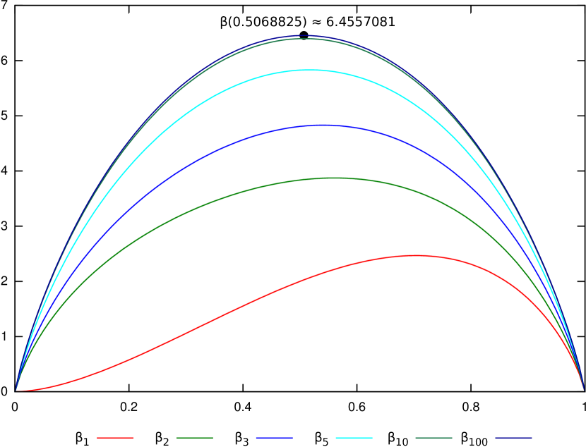
   Figure 1: The functions $\beta_{m}$ for $m=1,2,3,5,10,100$.

4. The function $\beta$ can be simplified a bit further. Observe that

   $$h\left(q_{m+1}\right) =h\left(\frac{1}{1+q_{m}}\right)=\frac{1}{1+q_{m}}\log_{2}\left(1+q_{m}\right)+\frac{q_{m}}{1+q_{m}}\log_{2}\frac{1+q_{m}}{q_{m}}$$

   $$=\log_{2}\left(1+q_{m}\right)-q_{m}q_{m+1}\log_{2}q_{m}=-\log_{2}q_{m+1}-q_{m}q_{m+1}\log_{2}q_{m},$$

   hence we can write

   $$\beta\left(z\right)=4zh\left(z\right)-4z\left(1-z\right)\sum_{m=0}^{\infty}\left(\pi_{m}\log_{2}q_{m+1}+\pi_{m+2}\log_{2}q_{m}\right).$$

5 A Lipschitz-type condition for total influence and entropy

In this section we show that changing a single entry in a Boolean function has a negligible effect on its total influence and entropy.

Lemma 5.1.

Let $f$ and $g$ be Boolean functions on $n$ variables differing in a single entry $x=x_{0}$. Then $\left|{\bf I}\left[f\right]-{\bf I}\left[g\right]\right|\leq 2n/N$.

Proof.

We use an equivalent definition of total influence as the average sensitivity

$${\bf I}\left[f\right]={\rm\mathbf{E}}\left[{\bf S}_{f}\left(x\right)\right]=\frac{1}{N}\sum_{x}{\bf S}_{f}\left(x\right),$$

where ${\bf S}_{f}\left(x\right)$ is the number of neighbors $y\sim x$ in the Boolean cube such that $f\left(x\right)\neq f\left(y\right)$. Indeed, we have

$$\left|{\bf S}_{f}\left(x\right)-{\bf S}_{g}\left(x\right)\right|\leq\begin{cases}n,&x=x_{0};\\ 1,&x\sim x_{0};\\ 0,&\text{otherwise}.\end{cases}$$

Thus,

$$\left|{\bf I}\left[f\right]-{\bf I}\left[g\right]\right|=\frac{1}{N}\left|\sum_{x}{\bf S}_{f}\left(x\right)-{\bf S}_{g}\left(x\right)\right|\leq\frac{1}{N}\sum_{x}\left|{\bf S}_{f}\left(x\right)-{\bf S}_{g}\left(x\right)\right|\leq\frac{2n}{N}.\qed$$

Remark.

This is tight. Indeed, ${\rm Or}_{n}$ differs from the all-${\bf true}$ function in a single entry $x={\bf false}^{n}$ and ${\bf I}\left[{\rm Or}_{n}\right]-{\bf I}\left[{\bf true}\right]=2n/N-0=2n/N$.

Lemma 5.2.

Let $f$ and $g$ be Boolean functions on $n$ variables differing in a single entry $x=x_{0}$. Then $\left|{\bf H}\left[f\right]-{\bf H}\left[g\right]\right|\leq 12n/\sqrt{N}$.

Proof.

This is trivial for $n=1$ so assume $n\geq 2$. Also assume without loss of generality that the differing entry is $x_{0}={\bf false}^{n}$; that is, $g=f+2\delta$, where

$$\delta\left(x\right)=\frac{1}{2}+\frac{1}{2}{\rm Or}_{n}\left(x\right)=\begin{cases}1,&x=x_{0};\\ 0,&x\neq x_{0}.\end{cases}$$

Write $a=\frac{N}{2}\left(f+g\right)=N\left(f+\delta\right)$, so $f=\frac{1}{N}a-\delta$ and thus $\hat{f}\left(S\right)=\frac{1}{N}\left(\hat{a}\left(S\right)-1\right)$. Similarly we have $g=\frac{1}{N}a+\delta$ and $\hat{g}\left(S\right)=\frac{1}{N}\left(\hat{a}\left(S\right)+1\right)$. In particular, we have

$$\sum_{S\subseteq\left[n\right]}\hat{a}\left(S\right) = N\left(\sum_{S\subseteq\left[n\right]}\hat{f}\left(S\right)\right)-N=0;$$

$$\sum_{S\subseteq\left[n\right]}\hat{a}\left(S\right)^{2} = \sum_{S\subseteq\left[n\right]}\left(N^{2}\hat{f}\left(S\right)^{2}+2N\hat{f}\left(S\right)+1\right)=N\left(N-1\right).$$

Fourier coefficients of Boolean functions on $n$ variables are known to reside in $\left\{\pm 2k/N\right\}_{k=0}^{N/2}$; thus the Fourier coefficients of $a$ belong to $\left\{\pm\left(2k-1\right)\right\}_{k=1}^{N/2}$. For $k\in\left[N/2\right]$ let

$$\Delta_{k}=\sum_{S:\left|\hat{a}\left(S\right)\right|=2k-1}{\rm sgn}\left(\hat{a}\left(S\right)\right)=\left|\left\{S:\hat{a}\left(S\right)=2k-1\right\}\right|-\left|\left\{S:\hat{a}\left(S\right)=1-2k\right\}\right|$$

and observe that

$$\sum_{k=1}^{N/2}\Delta_{k}\left(2k-1\right) = \sum_{S\subseteq\left[n\right]}\hat{a}\left(S\right)=0,$$ (9a)

$$\sum_{k=1}^{N/2}\left|\Delta_{k}\right| \leq \sum_{S\subseteq\left[n\right]}1=N,$$ (9b)

$$\sum_{k=1}^{N/2}\left|\Delta_{k}\right|\left(2k-1\right)^{2} \leq \sum_{S\subseteq\left[n\right]}\hat{a}\left(S\right)^{2}=N\left(N-1\right),$$ (9c)

$$\sum_{k=1}^{N/2}\left|\Delta_{k}\right|\left(2k-1\right) \leq \sqrt{\sum_{k=1}^{N/2}\left|\Delta_{k}\right|\cdot\sum_{k=1}^{N/2}\left|\Delta_{k}\right|\left(2k-1\right)^{2}}\leq N\sqrt{N-1}<N^{3/2},$$ (9d)

where Cauchy–Schwartz was used to derive (9d) from (9b) and (9c).

We express the difference of entropies in terms of $\left(\Delta_{k}\right)_{k\in\left[N/2\right]}$ (details in Appendix A):

$${\bf H}\left[f\right]-{\bf H}\left[g\right]=\frac{8}{N^{2}}\sum_{k=2}^{N/2}\Delta_{k}k^{2}\log_{2}\frac{k}{k-1}+\frac{8}{N^{2}}\sum_{k=2}^{N/2}\Delta_{k}\left(2k-1\right)\log_{2}\left(k-1\right).$$ (10)

To bound the first term, note that the function $\xi\left(x\right)=x^{2}\log_{2}\left(x/\left(1-x\right)\right)-\left(2x-1\right)/\ln 4$ is decreasing and positive for $x>1$, and $\xi\left(2\right)=4-3/\ln 4\approx 1.836$. Now

$$\Big{|}\sum_{k=2}^{N/2}\Delta_{k}k^{2}\log_{2}\frac{k}{k-1} \Big{|}=\Big{|}\sum_{k=2}^{N/2}\Delta_{k}\left(\xi(k)+\frac{2k-1}{\ln 4}\right)\Big{|}$$

$$\leq\frac{1}{\ln 4}\Big{|}\sum_{k=2}^{N/2}\Delta_{k}\left(2k-1\right)\Big{|}+\Big{|}\sum_{k=2}^{N/2}\Delta_{k}\xi(k)\Big{|}$$

[by (9a)] $$=\frac{1}{\ln 4}\left|\Delta_{1}\right|+\Big{|}\sum_{k=2}^{N/2}\Delta_{k}\xi(k)\Big{|}$$

$$\leq\frac{1}{\ln 4}\left|\Delta_{1}\right|+\sum_{k=2}^{N/2}\left|\Delta_{k}\right|\xi(2)$$

$$\leq\max\left\{\frac{1}{\ln 4},\xi(2)\right\}\sum_{k=1}^{N/2}\left|\Delta_{k}\right|$$

[by (9b)] $$\leq\max\left\{\frac{1}{\ln 4},\xi(2)\right\}N=\xi(2)N<2N.$$ (11)

To bound the second term, note that the function $\zeta\left(x\right)=x\log_{2}\frac{x-1}{2}$ is increasing, positive and convex for $x>3$, so

$$\Big{|}2\sum_{k=2}^{N/2}\Delta_{k}\left(2k-1\right)\log_{2}\left(k-1\right)\Big{|} =2\Big{|}\sum_{k=2}^{N/2}\Delta_{k}\zeta\left(2k-1\right)\Big{|}\leq 2\sum_{k=2}^{N/2}\left|\Delta_{k}\right|\zeta\left(2k-1\right)$$

[Jensen’s inequality] $$\leq 2\zeta\Big{(}\sum_{k=2}^{N/2}\left|\Delta_{k}\right|\left(2k-1\right)\Big{)}$$

[by (9d)] $$\leq 2\zeta\left(N^{3/2}\right)=2N^{3/2}\log_{2}\frac{N^{3/2}-1}{2}$$

$$<2N^{3/2}\left(3n/2-1\right)=3N^{3/2}n-2N^{3/2}.$$ (12)

Combining (10), (11) and (12), we get

$$\left|{\bf H}\left[f\right]-{\bf H}\left[g\right]\right|\leq\frac{8}{N^{2}}\cdot 2N+\frac{4}{N^{2}}\left(3N^{3/2}n-2N^{3/2}\right)\leq\frac{12n}{N},$$

establishing the proof of the lemma. ∎

Corollary.

Let $f$ and $g$ be Boolean functions on $n$ variables, and let $\epsilon={\rm Pr}\left[f\left(x\right)\neq g\left(x\right)\right]$. Then $\left|{\bf I}\left[f\right]-{\bf I}\left[g\right]\right|\leq 2\epsilon n$ and $\left|{\bf H}\left[f\right]-{\bf H}\left[g\right]\right|<12\epsilon n\sqrt{N}$.

Remark.

One may wonder how tight is Lemma 5.2, since the largest distance obtained from natural examples seems to be

$${\bf H}\left[{\rm Or}_{n}\right]-{\bf H}\left[{\bf true}\right]<8\left(n-1+1/\ln 4\right)/N-0<8n/N.$$

There exists, however, a algebraic construction in which the entropy difference is greater than $8/(3\sqrt{N})$, so the lemma is tight upto the logarithmic factor $n$:

Niho [8] considered functions from $\mathbb{GF}\left(N\right)$ to $\mathbb{GF}\left(2\right)$ of the form $f\left(\alpha\right)={\rm Tr}\left(\alpha^{r}\right)$, where ${\rm Tr}:\mathbb{GF}\left(N\right)\to\mathbb{GF}\left(2\right)$ is the trace operator and $r$ is some integer. These can naturally be interpreted as Boolean functions from $\left\{{\bf false},{\bf true}\right\}^{n}$ to $\left\{{\bf false},{\bf true}\right\}$.

The case when $n\equiv 0\bmod 4$ and $r=2\sqrt{N}-1$ was analyzed in [8, Theorem 3-6]. The Fourier spectrum of the resulting function $f$ has four possible values, as summarized in Table 2. Plugging these numbers in (10) shows that indeed ${\bf H}\left[f+2\delta\right]-{\bf H}\left[f\right]>8/(3\sqrt{N})$.

Value of $\hat{f}$	$-1/\sqrt{N}$	$0$	$1/\sqrt{N}$	$2/\sqrt{N}$
Multiplicity	$\frac{1}{3}(N-\sqrt{N})$	$\frac{1}{2}(N-\sqrt{N})$	$\sqrt{N}$	$\frac{1}{6}(N-\sqrt{N})$

Table 2: Spectrum of Niho’s function $f\left(\alpha\right)={\rm Tr}\big{(}\alpha^{2\sqrt{N}-1}\big{)}$ for $n\equiv 0\bmod 4$.

6 Concluding Remarks and Open Problems

1. The key element repeating in all our constructions is lexicographic functions:

   1. In Theorem 2.11 they allowed us to create a balanced function $\ell\left\langle 2/3\right\rangle\sqcap\ell\left\langle 3/4\right\rangle$ of positive entropy and small total influence that we could plug in Proposition 1.2;

   2. In Theorem 3.3, using $\ell\left\langle\Phi\right\rangle$ we converted uniform bits to $\left(1-2\Phi\right)$-biased bits that we could plug in the biased variant of Proposition 1.2 with the base function $\tau$;

   3. In Theorem 4.4, the constructed sequence had $\ell\left\langle 2/3\right\rangle$ as either its first or second member.

   This is far from being a coincidence, as lexicographic functions are the minimizers of total influence (for a given bias) by Theorem 2.3. It seems plausible to attempt proving Conjecture 1.1 for the class of monotone Boolean functions (or perhaps all Boolean functions) by proving an upper bound on what can be done using lexicographic functions.

2. It is possible that we can improve on Theorems 3.3 and 4.4 by finding a base function $g$ better than $\tau$. Of course, $g$ should be $\eta$-balanced for some $-1<\eta<1$; that is, $\eta$ should be a fixed point of $E_{g}\left(\rho\right)={\rm\mathbf{E}}_{x\sim\rho}\left[g\right]$. Preferably, $\eta$ should be an attractive fixed point of $E_{g}$, so $g$ needs to be a non-monotone function. By exhaustive search, we have determined that no function on $n\leq 4$ variables will do better than $\tau$.

   Nevertheless, all constructions based on disjoint composition belong to the class of read-once formulas, and thus cannot provide a lower bound better than 10.

3. One remaining gap worth closing is the asympotic behavior of the Lipschitz constant for the spectral entropy. Recall that Niho’s function gave a lower bound of $\Omega(1/\sqrt{N})$, whereas the upper bound provided by Lemma 5.2 is $O(n/\sqrt{N})$. We believe the upper bound is not tight.

Appendix A Boring Calculations

A.1 From Section 1

Proof of Claim 1.3.

By induction on $m$. It is true for $m=1$ since

$${\rm Pr}\left[x_{1}\mid x_{1}\vee x_{2}\right]={\rm Pr}\left[x_{1}\wedge\left(x_{1}\vee x_{2}\right)\right]/{\rm Pr}\left[x_{1}\vee x_{2}\right]=\frac{1/2}{3/4}=2/3.$$

Assuming correctness for $m$, we have

$${\rm Pr}\left[G_{m+1}\left(x_{3},\ldots,x_{2m+2},x_{1}\right)\mid x_{1}\vee x_{2}\right]$$

$$\quad={\rm Pr}\left[x_{3}\vee\left(x_{4}\wedge G_{m}\left(x_{5},\ldots,x_{2m+2},x_{1}\right)\right)\mid x_{1}\vee x_{2}\right]$$

$$\quad=1-\left(1-\frac{1}{2}\right)\left(1-\frac{1}{2}\cdot{\rm Pr}\left[G_{m}\left(x_{5},\ldots,x_{2m+2},x_{1}\right)\mid x_{1}\vee x_{2}\right]\right)$$

$$\quad=1-\frac{1}{2}\left(1-\frac{1}{2}\cdot\frac{2}{3}\right)=\frac{1}{2}+\frac{1}{6}=\frac{2}{3}.\qed$$

A.2 From Section 2

Proof of Claim 2.5.

By induction on $t$. It trivially holds for $t=0$. Assuming correctness for $t$, let $s^{\prime}=s-N/2^{k_{0}}$. By Proposition 2.4

$${\bf I}\left[\ell_{n}\left\langle s\right\rangle\right] =\frac{2sn}{N}-\frac{4}{N}\sum_{x=0}^{s-1}wt\left(x\right)$$

$$=\frac{2n}{N}\cdot\frac{N}{2^{k_{0}}}+\frac{2s^{\prime}n}{N}-\frac{4}{N}\sum_{x=0}^{N/2^{k_{0}}-1}wt\left(x\right)-\frac{4}{N}\sum_{x=N/2^{k_{0}}}^{s-1}wt\left(x\right)$$

$$=\frac{n}{2^{k_{0}-1}}-\frac{4}{N}\frac{N}{2^{k_{0}}}\frac{n-k_{0}}{2}+\frac{2s^{\prime}n}{N}-\frac{4}{N}\sum_{x=0}^{s^{\prime}-1}\left(1+wt\left(x\right)\right)$$

$$=\frac{n}{2^{k_{0}-1}}-\frac{n-k_{0}}{2^{k_{0}-1}}+{\bf I}\left[\ell_{n}\left\langle s^{\prime}\right\rangle\right]-\frac{4s^{\prime}}{N}$$

$$=k_{0}2^{1-k_{0}}+\sum_{i=1}^{t+1}\left(k_{i}-2i+2\right)2^{1-k_{i}}-\frac{4}{N}\sum_{i=1}^{t+1}N/2^{k_{i}}$$

$$=\sum_{i=0}^{t+1}\left(k_{i}-2i\right)2^{1-k_{i}}.\qed$$

Proof of Claim 2.7.

(A full computation of ${\bf I}\left[\ell\left\langle\mu\right\rangle\right]$ for the case $\mu<\frac{1}{4}$) Recall that $k_{i}=i+3$ for $i<j$ and $k_{i}\geq i+4$ for $i\geq j$. Thus,

$${\bf I}\left[\ell\left\langle\mu\right\rangle\right] =\sum_{i=0}^{\infty}\left(k_{i}-2i\right)2^{1-k_{i}}$$

$$=\sum_{i=0}^{j-1}\left(i+3-2i\right)2^{1-i-3}+\sum_{i=j}^{\infty}\left(k_{i}-2i\right)2^{-1-k_{i}}$$

$$\leq\frac{1}{4}\sum_{i=0}^{j-1}\left(3-i\right)2^{-i}+2\sum_{i=j}^{\infty}\left(k_{i}-2j\right)2^{-k_{i}}$$

$$\leq\frac{3}{4}\sum_{i=0}^{j-1}2^{-i}-\frac{1}{4}\sum_{i=0}^{j-1}i2^{-i}+2\sum_{i=j+4}^{\infty}\left(i-2j\right)2^{-i}$$

$$=\frac{3}{2}\left(1-2^{-j}\right)-\frac{1}{4}\left(2-\sum_{i=j}^{\infty}i2^{-i}\right)+2\sum_{i=j+4}^{\infty}i2^{-i}-4j\sum_{i=j+4}^{\infty}2^{-i}$$

$$=1-3\cdot 2^{-j-1}+\frac{1}{4}\left(j+1\right)2^{1-j}+2\left(j+4+1\right)2^{1-j-4}-4j\cdot 2^{1-j-4}$$

$$=1+2^{-j-2}\left(j+1\right)\leq\frac{5}{4}<\frac{4}{3},$$

where in the second to last equality we used the identity $\sum_{i=j}^{\infty}i2^{-i}=\left(j+1\right)2^{1-j}$. ∎

Proof of Claim 2.9.

We have

$$2-2h\left(p/2\right) =2+2\frac{p}{2}\log_{2}\frac{p}{2}+2\left(1-\frac{p}{2}\right)\log_{2}\left(1-\frac{p}{2}\right)$$

$$=p\log_{2}p+\left(2-p\right)\log_{2}\left(2-p\right)$$

so

$$\psi\left(p,1/2\right)= \tilde{h}\left(p/2\right)+2p\left(h\left(p\right)+1-h\left(p/2\right)\right)$$

$$= -\left(1-p\right)^{2}\log_{2}\left(\left(1-p\right)^{2}\right)-\left(2p-p^{2}\right)\log_{2}\left(2p-p^{2}\right)$$

$$+2ph\left(p\right)+p^{2}\log_{2}p+p\left(2-p\right)\log_{2}\left(2-p\right)$$

$$= 2ph\left(p\right)-2\left(1-p\right)^{2}\log_{2}\left(1-p\right)-p\left(2-p\right)\log_{2}p+p^{2}\log_{2}p$$

$$= 2ph\left(p\right)-2\left(1-p\right)\left(\left(1-p\right)\log_{2}\left(1-p\right)+p\log_{2}p\right)=2h\left(p\right).\qed$$

A full computation of $H_{*}$:

$$H_{*} ={\bf H}\left[g\right]={\bf H}\left[{\rm Or}_{2}\sqcap G\right]$$

$$=\frac{2}{3}\left({\bf H}\left[{\rm Or}_{2}\right]-\tilde{h}\left(3/4\right)\right)+\frac{3}{4}\left({\bf H}\left[G\right]-\tilde{h}\left(2/3\right)\right)+\psi\left(3/4,2/3\right)$$

$$=\frac{2}{3}\left(2-h\left(1/4\right)\right)+\frac{3}{4}\left(2\log_{2}3-h\left(1/9\right)\right)+\tilde{h}\left(1/2\right)+2\left(h\left(3/4\right)+h\left(2/3\right)-h\left(1/2\right)\right)$$

$$=\frac{4}{3}+\left(2-\frac{2}{3}\right)h\left(1/4\right)+\frac{3}{4}\cdot\frac{8}{3}+0+2h\left(1/3\right)-2\cdot 1$$

$$=\frac{4}{3}+\frac{4}{3}\left(2-\frac{3}{4}\log_{2}3\right)+2\left(\log_{2}3-\frac{2}{3}\right)=\frac{8}{3}+\log_{2}3.$$

A.3 From Section 3

A full computation of $\tilde{{\bf H}}\left[\tau\right]$ for the bias $\eta=1-2\Phi$:

$$\tilde{{\bf H}}\left[\tau\right] =-\Phi^{6}\log_{2}\Phi^{6}-2\cdot 4\Phi^{5}\log_{2}(4\Phi^{5})-4\Phi^{6}\log_{2}(4\Phi^{6})$$

$$=-\Phi^{5}\left(6\Phi\log_{2}\Phi+40\log_{2}\Phi+16+8\Phi+24\Phi\log_{2}\Phi\right)$$

$$=-8\Phi^{5}\left(2+\Phi\right)-10\left(3\Phi+4\right)\Phi^{5}\log_{2}\Phi$$

$$=8\left(1-2\Phi\right)+10\left(4\Phi-3\right)\log_{2}\Phi.$$

Proof of Claim 3.2.

Recall that earlier we computed $\tilde{{\bf I}}\left[\tau\right]=8\Phi^{4}$. By Lemma 3.1,

$${\bf I}\left[F_{m+1}\right] =\tilde{{\bf I}}\left[\tau\right]{\bf I}^{+}\left[F_{m}\right]=\tilde{{\bf I}}\left[\tau\right]\frac{{\bf I}\left[F_{m}\right]}{{\rm\mathbf{Var}}\left[F_{m}\right]}$$

$$=\frac{8\Phi^{4}}{4\Phi^{3}}\cdot{\bf I}\left[F_{m}\right]=2\Phi\cdot{\bf I}\left[F_{m}\right].$$

Furthermore,

$$\frac{{\bf H}^{+}\left[F_{m+1}\right]}{{\bf I}^{+}\left[F_{m+1}\right]} =\frac{{\bf H}\left[F_{m+1}\right]-\tilde{h}\left(\Phi\right)}{{\bf I}\left[F_{m+1}\right]}$$

$$=\frac{\tilde{{\bf I}}\left[\tau\right]\cdot{\bf H}^{+}\left[F_{m}\right]}{\tilde{{\bf I}}\left[\tau\right]\cdot{\bf I}^{+}\left[F_{m}\right]}+\frac{\tilde{{\bf H}}\left[\tau\right]-\tilde{h}\left(\Phi\right)}{{\bf I}\left[F_{m+1}\right]},$$

hence

$$\frac{{\bf H}^{+}\left[F_{m}\right]}{{\bf I}^{+}\left[F_{m}\right]} =\frac{{\bf H}^{+}\left[F_{0}\right]}{{\bf I}^{+}\left[F_{0}\right]}+\left(\tilde{{\bf H}}\left[\tau\right]-\tilde{h}\left(\Phi\right)\right)\sum_{k=1}^{m}\frac{1}{{\bf I}\left[F_{k}\right]}$$

$$=\frac{{\bf H}^{+}\left[F_{0}\right]}{{\bf I}^{+}\left[F_{0}\right]}+\frac{\tilde{{\bf H}}\left[\tau\right]-\tilde{h}\left(\Phi\right)}{{\bf I}\left[F_{0}\right]}\sum_{k=1}^{m}\left(2\Phi\right)^{-k}$$

$$=\frac{{\bf H}^{+}\left[\ell\left\langle\Phi\right\rangle\right]}{{\bf I}^{+}\left[\ell\left\langle\Phi\right\rangle\right]}+\frac{\tilde{{\bf H}}\left[\tau\right]-\tilde{h}\left(\Phi\right)}{{\bf I}\left[\ell\left\langle\Phi\right\rangle\right]}\cdot\frac{1-\left(2\Phi\right)^{-m}}{2\Phi-1}.$$

Asymptotically the $\left(2\Phi\right)^{-m}$ term disappears, and we have

$$\lim_{m\to\infty}\frac{{\bf H}\left[F_{m}\right]}{{\bf I}\left[F_{m}\right]} =\lim_{m\to\infty}\frac{{\bf H}^{+}\left[F_{m}\right]-\tilde{h}\left(\Phi\right)}{{\bf I}^{+}\left[F_{m}\right]}=\lim_{m\to\infty}\frac{{\bf H}^{+}\left[F_{m}\right]}{{\bf I}^{+}\left[F_{m}\right]}-0$$

$$=\frac{{\bf H}^{+}\left[\ell\left\langle\Phi\right\rangle\right]}{{\bf I}^{+}\left[\ell\left\langle\Phi\right\rangle\right]}+\frac{\tilde{{\bf H}}\left[\tau\right]-\tilde{h}\left(\Phi\right)}{\left(2\Phi-1\right){\bf I}\left[\ell\left\langle\Phi\right\rangle\right]}$$

$$=\frac{{\bf H}\left[\ell\left\langle\Phi\right\rangle\right]-\tilde{h}\left(\Phi\right)}{{\bf I}\left[\ell\left\langle\Phi\right\rangle\right]}+\frac{\tilde{{\bf H}}\left[\tau\right]-\tilde{h}\left(\Phi\right)}{\left(2\Phi-1\right){\bf I}\left[\ell\left\langle\Phi\right\rangle\right]}$$

$$=\frac{{\bf H}\left[\ell\left\langle\Phi\right\rangle\right]+\left(3+2\Phi\right)\tilde{{\bf H}}\left[\tau\right]-\left(4+2\Phi\right)\tilde{h}\left(\Phi\right)}{{\bf I}\left[\ell\left\langle\Phi\right\rangle\right]}.\qed$$

A.4 From Section 4

Proof of Proposition 4.1.

We have

$${\rm Pr}\left[\kappa\right]=1-{\rm Pr}\left[\lambda\sqcap\kappa\right]=1-p{\rm Pr}\left[\kappa\right],$$

so we can solve for

$$q={\rm Pr}\left[\kappa\right]=\frac{1}{1+p}.$$

Next, by Proposition 2.8 and duality we have

$${\bf I}\left[\kappa\right] ={\bf I}\left[\lambda\sqcap\kappa\right]=q{\bf I}\left[\lambda\right]+p{\bf I}\left[\kappa\right]$$

and we can solve for ${\bf I}\left[\kappa\right]=q{\bf I}\left[\lambda\right]/\left(1-p\right),$yielding

$${\bf I}^{+}\left[\kappa\right]=\frac{{\bf I}\left[\kappa\right]}{4q\left(1-q\right)}=\frac{q{\bf I}\left[\lambda\right]}{4q\cdot pq\cdot\left(1-p\right)}=\frac{1}{q}{\bf I}^{+}\left[\lambda\right].$$

Last, we compute ${\bf H}\left[\kappa\right]$. Note that since $q=1-pq$ we have $h\left(pq\right)=h\left(q\right)$ and $\tilde{h}\left(pq\right)=\tilde{h}\left(q\right)$, so

$$\psi\left(p,q\right) =\tilde{h}\left(pq\right)+4pq\left(h\left(p\right)+h\left(q\right)-h\left(pq\right)\right)$$

$$=\tilde{h}\left(q\right)+4pqh\left(p\right).$$

Now, by Proposition 2.8,

$${\bf H}\left[\kappa\right] ={\bf H}\left[\lambda\sqcap\kappa\right]=q\left({\bf H}\left[\lambda\right]-\tilde{h}\left(p\right)\right)+p\left({\bf H}\left[\kappa\right]-\tilde{h}\left(q\right)\right)+\psi\left(p,q\right)$$

$$=p{\bf H}\left[\kappa\right]+q\left({\bf H}\left[\lambda\right]-\tilde{h}\left(p\right)\right)-p\tilde{h}\left(q\right)+\tilde{h}\left(q\right)+4pqh\left(p\right)$$

so we can solve for

$${\bf H}\left[\kappa\right] =\frac{q\left({\bf H}\left[\lambda\right]-\tilde{h}\left(p\right)\right)+\left(1-p\right)\tilde{h}\left(q\right)+4pqh\left(p\right)}{1-p}$$

$$=\frac{q}{1-p}\left({\bf H}\left[\lambda\right]-\tilde{h}\left(p\right)+4ph\left(p\right)\right)+\tilde{h}\left(q\right),$$

yielding

$${\bf H}^{+}\left[\kappa\right] =\frac{{\bf H}\left[\kappa\right]-\tilde{h}\left(q\right)}{4q\left(1-q\right)}=\frac{{\bf H}\left[\lambda\right]-\tilde{h}\left(p\right)+4ph\left(p\right)}{4\left(1-p\right)\cdot pq}$$

$$=\frac{{\bf H}\left[\lambda\right]-\tilde{h}\left(p\right)}{4p\left(1-p\right)q}+\frac{h\left(p\right)}{\left(1-p\right)q}$$

$$=\left({\bf H}^{+}\left[\lambda\right]+\frac{h\left(p\right)}{1-p}\right)/q.\qed$$

Proof of Claim 4.2.

For $m=0$ indeed $q_{m}=\left(1\cdot z+0\right)/\left(0\cdot z+1\right)=z$. Now, assuming the claim holds for $q_{m}$,

$$q_{m+1} =\frac{1}{1+q_{m}}=\frac{b_{m}z+b_{m+1}}{\left(b_{m}z+b_{m+1}\right)\left(1+q_{m}\right)}$$

$$=\frac{b_{m}z+b_{m+1}}{b_{m}z+b_{m+1}+b_{m-1}z+b_{m}}$$

$$=\frac{b_{m}z+b_{m+1}}{\left(b_{m}+b_{m-1}\right)z+\left(b_{m+1}+b_{m}\right)}$$

$$=\frac{b_{m}z+b_{m+1}}{b_{m+1}z+b_{m+2}}.\qed$$

Proof of Claim 4.3.

By (3b) and (3c),

$$\frac{{\bf H}^{+}\left[F_{k+1}\right]}{{\bf I}^{+}\left[F_{k+1}\right]} =\frac{{\bf H}^{+}\left[F_{k}\right]}{{\bf I}^{+}\left[F_{k}\right]}+\frac{h\left(q_{k}\right)}{\left(1-q_{k}\right){\bf I}^{+}\left[F_{k}\right]}$$

$$=\frac{{\bf H}^{+}\left[F_{k}\right]}{{\bf I}^{+}\left[F_{k}\right]}+\frac{h\left(q_{k}\right)\pi_{k}}{\left(1-q_{k}\right){\bf I}^{+}\left[F_{0}\right]}$$

$$=\frac{{\bf H}^{+}\left[F_{k}\right]}{{\bf I}^{+}\left[F_{k}\right]}+\frac{h\left(q_{k}\right)\pi_{k-2}}{{\bf I}^{+}\left[F_{0}\right]},$$

thus

$$\frac{{\bf H}^{+}\left[F_{m}\right]}{{\bf I}^{+}\left[F_{m}\right]} =\frac{{\bf H}^{+}\left[F_{0}\right]}{{\bf I}^{+}\left[F_{0}\right]}+\sum_{k=0}^{m-1}\frac{{\bf H}^{+}\left[F_{k+1}\right]}{{\bf I}^{+}\left[F_{k+1}\right]}-\frac{{\bf H}^{+}\left[F_{k}\right]}{{\bf I}^{+}\left[F_{k}\right]}$$

$$=\frac{{\bf H}^{+}\left[F_{0}\right]}{{\bf I}^{+}\left[F_{0}\right]}+\sum_{k=-2}^{m-3}\frac{h\left(q_{k+2}\right)\pi_{k}}{{\bf I}^{+}\left[F_{0}\right]}$$

and

$$\frac{{\bf H}\left[F_{m}\right]}{{\bf I}\left[F_{m}\right]} =\frac{{\bf H}^{+}\left[F_{m}\right]}{{\bf I}^{+}\left[F_{m}\right]}+\frac{\tilde{h}\left(q_{m}\right)}{{\bf I}\left[F_{m}\right]}$$

$$=\frac{{\bf H}^{+}\left[F_{m}\right]}{{\bf I}^{+}\left[F_{m}\right]}+\frac{\tilde{h}\left(q_{m}\right)}{4q_{m}\left(1-q_{m}\right){\bf I}^{+}\left[F_{m}\right]}$$

$$=\frac{{\bf H}^{+}\left[F_{0}\right]}{{\bf I}^{+}\left[F_{0}\right]}+\frac{\tilde{h}\left(q_{m}\right)\pi_{m-2}}{4q_{m}{\bf I}^{+}\left[F_{0}\right]}+\sum_{k=-2}^{m-3}\frac{h\left(q_{k+2}\right)\pi_{k}}{{\bf I}^{+}\left[F_{0}\right]}$$

$$=\frac{H-\tilde{h}\left(z\right)}{I}+\frac{4z\left(1-z\right)}{I}\left(\frac{1+q_{m-1}}{4}\tilde{h}\left(q_{m}\right)\pi_{m-2}+\sum_{k=-2}^{m-3}h\left(q_{k+2}\right)\pi_{k}\right)\cdot$$

$$=\frac{1}{I}\left(H-\tilde{h}\left(z\right)+z\left(1-z\right)\left(\pi_{m-1}+\pi_{m-2}\right)\tilde{h}\left(q_{m}\right)+\beta_{m}\left(z\right)\right).\qed$$

A.4.1 Lower bound obtained from $T=\left(T\sqcap T\right)^{\dagger}$

First we prove an analogue of Proposition 4.1:

Given a Boolean function $\lambda$, define $\kappa=\left(\lambda\sqcap\lambda\right)^{\dagger}$. Writing $p={\rm Pr}\left[\lambda\right]$ and $q={\rm Pr}\left[\kappa\right]$ we have $q=1-p^{2}.$ By Proposition 2.8 we have

$${\bf I}\left[\kappa\right] ={\bf I}\left[\lambda\sqcap\lambda\right]=2p{\bf I}\left[\lambda\right],$$

$${\bf H}\left[\kappa\right] ={\bf H}\left[\lambda\sqcap\lambda\right]=2p\left({\bf H}\left[\lambda\right]-\tilde{h}\left(p\right)\right)+\psi\left(p,p\right)$$

$$=2p\left({\bf H}\left[\lambda\right]-\tilde{h}\left(p\right)\right)+\tilde{h}\left(p^{2}\right)+4p^{2}\left(2h\left(p\right)-h\left(p^{2}\right)\right)$$

$$=2p\left({\bf H}\left[\lambda\right]-\tilde{h}\left(p\right)\right)+\tilde{h}\left(q\right)+8p^{2}h\left(p\right)-4p^{2}h\left(q\right).$$

Let $\tilde{C}_{m}=\left({\bf H}\left[T_{m}\right]-\tilde{h}\left(t_{m}\right)\right)/{\bf I}\left[T_{m}\right]$, where $t_{m}={\rm Pr}\left[T_{m}\right]$ . Now

$$\tilde{C}_{m+1}-\tilde{C}_{m} =\frac{8p^{2}h\left(p\right)-4p^{2}h\left(q\right)}{{\bf I}\left[T_{m+1}\right]}=\frac{4ph\left(p\right)}{{\bf I}\left[T_{m}\right]}-\frac{4\left(1-q\right)h\left(q\right)}{{\bf I}\left[T_{m+1}\right]}$$

so

$$\lim_{m\to\infty}\frac{{\bf H}\left[T_{m}\right]}{{\bf I}\left[T_{m}\right]} =\tilde{C}_{0}+\sum_{k=0}^{\infty}\left(\tilde{C}_{k+1}-\tilde{C}_{k}\right)=\frac{{\bf H}\left[T_{0}\right]-\tilde{h}\left(t_{0}\right)+\gamma\left(t_{0}\right)}{{\bf I}\left[T_{0}\right]},$$

where

$$\gamma\left(z\right) =4\sum_{k=0}^{\infty}\frac{t_{k}h\left(t_{k}\right)}{2^{k}\prod_{i=0}^{k-1}t_{i}}-4\sum_{k=1}^{\infty}\frac{\left(1-t_{k}\right)h\left(t_{k}\right)}{2^{k}\prod_{i=0}^{k-1}t_{i}}$$

$$=4zh\left(z\right)+4\sum_{k=1}^{\infty}\frac{\left(2t_{k}-1\right)h\left(t_{k}\right)}{2^{k}\prod_{i=0}^{k-1}t_{i}}.$$

A.5 From Section 5

The difference in entropies is:

$${\bf H}\left[f\right]-{\bf H}\left[g\right] =\sum_{S}\hat{g}\left(S\right)^{2}\log_{2}\left(\hat{g}\left(S\right)^{2}\right)-\hat{f}\left(S\right)^{2}\log_{2}\left(\hat{f}\left(S\right)^{2}\right)$$

$$=\frac{2}{N^{2}}\sum_{S}\left(N\hat{g}\left(S\right)\right)^{2}\log_{2}\left|\hat{g}\left(S\right)\right|-(N\hat{f}\left(S\right))^{2}\log_{2}|\hat{f}\left(S\right)|$$

$$=\frac{2}{N^{2}}\sum_{S}\Big{[}\left(\hat{a}\left(S\right)+1\right)^{2}\log_{2}\left(\left|\hat{a}\left(S\right)+1\right|/N\right)$$

$$\qquad\quad-\left(\hat{a}\left(S\right)-1\right)^{2}\log_{2}\left(\left|\hat{a}\left(S\right)-1\right|/N\right)\Big{]}$$

$$=\frac{2}{N^{2}}\sum_{S}\Big{[}\left(1+\hat{a}\left(S\right)\right)^{2}\log_{2}\left(\left|1+\hat{a}\left(S\right)\right|/N\right)$$

$$\qquad\quad-\left(1-\hat{a}\left(S\right)\right)^{2}\log_{2}\left(\left|1-\hat{a}\left(S\right)\right|/N\right)\Big{]}$$

$$=\frac{2}{N^{2}}\sum_{k=1}^{N/2}\Delta_{k}\left[\left(2k\right)^{2}\log_{2}\left(2k/N\right)-\left(2k-2\right)^{2}\log_{2}\left(2\left(k-1\right)/N\right)\right]$$

$$=\frac{8}{N^{2}}\sum_{k=1}^{N/2}\Delta_{k}\left[k^{2}\log_{2}k-\left(k-1\right)^{2}\log_{2}\left(k-1\right)\right]$$

$$\qquad-\frac{8\left(n-1\right)}{N^{2}}\sum_{k=1}^{N/2}\Delta_{k}\left[k^{2}-\left(k-1\right)^{2}\right]$$

[by (9a)] $$=\frac{8}{N^{2}}\sum_{k=1}^{N/2}\Delta_{k}\left[k^{2}\log_{2}k-\left(k-1\right)^{2}\log_{2}\left(k-1\right)\right]$$

[note the index $$k =\frac{8}{N^{2}}\sum_{k=2}^{N/2}\Delta_{k}\left[k^{2}\log_{2}k-\left(k-1\right)^{2}\log_{2}\left(k-1\right)\right]$$]

$$=\frac{8}{N^{2}}\sum_{k=2}^{N/2}\Delta_{k}k^{2}\log_{2}\frac{k}{k-1}+\frac{8}{N^{2}}\sum_{k=2}^{N/2}\Delta_{k}\left(2k-1\right)\log_{2}\left(k-1\right).$$

References

- [1] Sourav Chakraborty, Raghav Kulkarni, Satyanarayana V. Lokam, and Nitin Saurabh, Upper bounds on Fourier entropy. In: Proc. of the 21st International Computing and Combinatorics Conference (COCOON), pp. 771-782, 2015.
- [2] A.J. Bernstein, Maximally connected arrays on the -cube. SIAM J. Appl. Math. 15, pp. 1485–1489, 1967.
- [3] Bireswar Das, Manjish Pal, Vijay Visavaliya, The Entropy Influence conjecture revisited. Electronic Colloquium on Computational Complexity (ECCC) 18, #146, 2011.
- [4] Ehud Friedgut and Gil Kalai, Every monotone graph property has a sharp threshold. Proc. Amer. Math. Soc. 124(10), pp. 2993–3002, 1996.
- [5] L.H. Harper, Optimal assignment of numbers to vertices. J. Soc. Indust. Appl. Math. 12, pp. 131–135, 1964.
- [6] Sergiu Hart, A note on the edges of the -cube. Discr. Math. 14, pp. 157–163, 1976.
- [7] John H. Lindsey II, Assignment of numbers to vertices. Amer. Math. Monthly 7, pp. 508–516, 1964.
- [8] Yoji Niho, Multi-valued cross-correlation functions between two maximal linear recursive sequences. Ph.D. thesis, University of Southern California, Los Angeles, 1972.
- [9] Ryan O’Donnell and Li-Yang Tan, A composition theorem for the Fourier Entropy Influence conjecture. In: Proc. of the 40th International Colloquium on Automata, Language and Programming (ICALP), pp. 780–791, 2013.
- [10] Ryan O’Donnell, John Wright and Yuan Zhou, The Fourier Entropy Influence conjecture for certain classes of boolean functions. In: Proc. of the 38th International Colloquium on Automata, Language and Programming (ICALP), pp. 330–341, 2011.
- [11] Andrew Wan, John Wright, Chenggang Wu, Decision trees, protocols and the Entropy Influence conjecture. In: Proc. of the 5th conference on Innovations in Theoretical Computer Science (ITCS), pp. 67–80, 2014.