High-fidelity quantum gates in Si/SiGe double quantum dots

Abstract

Motivated by recent experiments of  Zajac et al. , we theoretically describe high-fidelity two-qubit gates using the exchange interaction between the spins in neighboring quantum dots subject to a magnetic field gradient. We use a combination of analytical calculations and numerical simulations to provide the optimal pulse sequences and parameter settings for the gate operation. We present a novel synchronization method which avoids detrimental spin flips during the gate operation and provide details about phase mismatches accumulated during the two-qubit gates which occur due to residual exchange interaction, non-adiabatic pulses, and off-resonant driving. By adjusting the gate times, synchronizing the resonant and off-resonant transitions, and compensating these phase mismatches by phase control, the overall gate fidelity can be increased significantly.

I Introduction

Spin qubits Loss and DiVincenzo (1998) implemented in silicon quantum dots Zwanenburg et al. (2013) are a viable candidate for enabling quantum error corrected quantum computation due to their long coherence times Steger et al. (2012); Tyryshkin et al. (2012); Veldhorst et al. (2014, 2015) and high-fidelity qubit manipulation Takeda et al. (2016); Zajac et al. ; Watson et al. . Experiments using isotopically enriched silicon show single-qubit fidelities $F>99.9\%$ Yoneda et al. thus exceeding the threshold of quantum-error correction Lidar and Brun (2013). Successful demonstrations of two-qubit gatesBrunner et al. (2011); Veldhorst et al. (2015); Zajac et al. ; Watson et al. , however, show fidelities far below the fault-tolerant threshold, therefore being the limiting factor for large-scale quantum computation. Here, based on the state-of-the-art quantum devicesZajac et al. (2016), we show a way to implement high-speed and high-fidelity two-qubit gates.

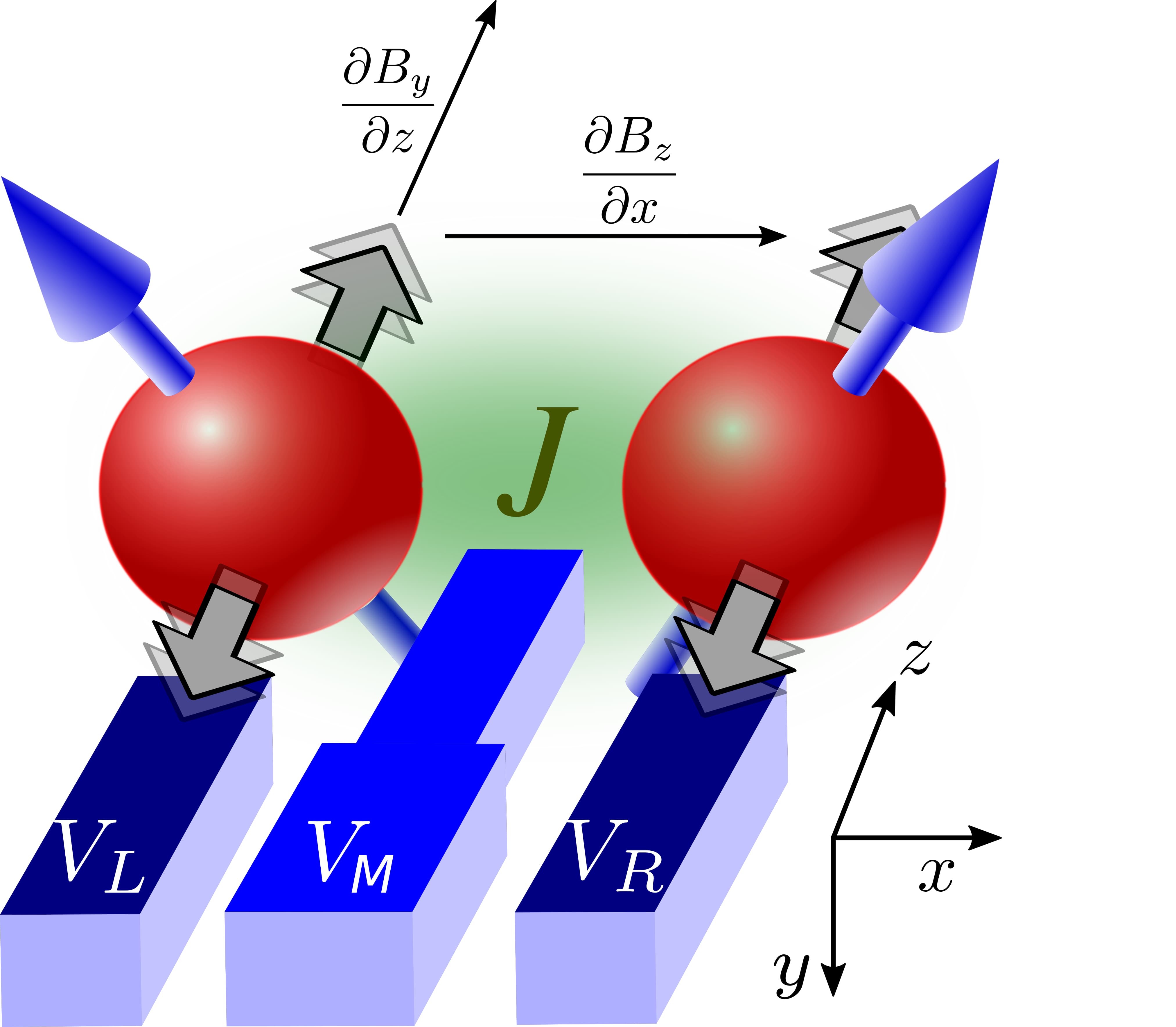
Figure 1: Illustration of a gate defined double quantum dot (DQD) occupied with two electron spins inside a large homogenous magnetic field (not shown) and an anisotropic magnetic field $\boldsymbol{B}$ from a micromagnet. A gradient $\frac{\partial B_{z}}{\partial x}$ along the double dot axis ($x$-direction) gives rise to distinguishable spin resonance frequencies. Periodic modulation of the gate voltages ($V_{L}$ and $V_{R}$) shifts the electron position in the $z$-direction (in plane) which in the motion-frame of the electrons “acts” as an oscillating magnetic field due to the gradient $\frac{\partial B_{y}}{\partial z}$. An electrostatic barrier gate $V_{M}$ allows for precise control over the exchange interaction $J$ between the spins.

High-speed and high-fidelity single-qubit gate operations are achieved using electric dipole spin resonance (EDSR) by shifting the electron position in a slanting magnetic field through the modulation of the electrostatic gate voltages Pioro-Ladriere et al. (2008); Brunner et al. (2011); Otsuka et al. (2016); Yoneda et al. ; Zajac et al. ; Watson et al. . Interconnecting multiple spin qubits is possible through the exchange interaction between electrons in adjacent quantum dots Loss and DiVincenzo (1998); Burkard et al. (1999a); Das Sarma et al. (2011). However, the fidelity of these gates is strongly limited by charge noise, which is induced by electric fluctuations of the system, and gives rise to substantial gate operation errors Petta et al. (2005); Brunner et al. (2011). Higher fidelities can be achieved if the system is operated at a symmetric operation point or sweet spot, where the exchange coupling is first-order insensitive to these fluctuations Bertrand et al. (2015); Martins et al. (2016); Reed et al. (2016); Zhang et al. (2017); Yang and Wang (2017). Alternatively, combining exchange with a strong magnetic field gradient between the electron spins in the dot Zajac et al. ; Watson et al. suppresses the dominating dephasing processes through the large energy splitting of the two-qubit states Nichol et al. (2017). Two explicit implementations for two-qubit gates have been successfully demonstrated, an ac pulsed frequency-selective CNOT gate Zajac et al. ; Watson et al. and a dc pulsed CPHASE gate Burkard et al. (1999b); Meunier et al. (2011); Watson et al. . These realizations are still not perfect, both acquiring local phases on the individual spin during the gate-operation due to unitary and non-unitary effects, e.g. charge noise, which have to be identified and compensated. The reduction of the overall gate fidelity due to off-resonant driving still remains an issue without the use of complex pulse shaping Economou and Barnes (2015); Ku et al. .

In this paper, we propose to implement high-fidelity dc CPHASE gates by adding an echo pulse and ac pulsed frequency-selective CNOT gate by synchronizing the resonant and off-resonant Rabi frequencies. We also identify local phases that the individual spins acquire during the CPHASE and CNOT operation due to the influence of the exchange interaction and the resonant and off-resonant driving. The paper is structured as follows. In section II, we begin with the theoretical description of our system. Subsequently, we model the dc pulsed CPHASE gate (section III) and present a high-fidelity implementation in subsection III.1. Then, we describe the ac pulsed frequency-selective CNOT gate (section IV), provide a synchronized high-fidelity implementation in subsection IV.1, and show its performance under the influence of charge noise in subsection IV.2. In section V, we conclude our paper with a summary and an outlook.

II Theoretical model

Our theoretical investigation is inspired by the experiments of Ref. Zajac et al. , therefore, we use the same terminology for the theoretical description. The setup (see Fig. 1) consists of two gate defined quantum dots in a Si/SiGe heterostructure operated in the (1,1) regime where $(n_{L},n_{R})$ is defined as the charge configuration with $n_{L}$ electrons in the left and $n_{R}$ electrons in the right dot. A middle barrier gate is biased with voltage $V_{M}$ to tune the exchange interaction $J$ between the two spins. For our theoretical description we use the Heisenberg Hamiltonian of two neighboring spins that are placed in an inhomogeneous magnetic field

$$H=J(t)(\boldsymbol{S}_{L}\cdot\boldsymbol{S}_{R}-1/4)+\boldsymbol{S}_{L}\cdot\boldsymbol{B}_{L}+\boldsymbol{S}_{R}\cdot\boldsymbol{B}_{R}.$$ (1)

Here $J$ describes the Heisenberg exchange interaction between the spin in the left dot, $\boldsymbol{S}_{L}$, and the spin in the right dot, $\boldsymbol{S}_{R}$, resulting from the hybridization of the singlet electron wave-function with additional charge states, (2,0) and (0,2). In the Hubbard limit, in the (1,1) charge configuration, exchange is given by $J=2t_{M}^{2}(U_{L}+U_{R})/[(U_{L}+\varepsilon)(U_{R}-\varepsilon)]$ where $t_{M}=t_{M}(V_{M})$ is the tunneling matrix element between the electron spins which depends on the middle barrier voltage $V_{M}$, $\varepsilon=(V_{L}-V_{R})/2$ is the single-particle detuning between the energy levels of the two spins set by $V_{L}$ and $V_{R}$, and $U_{L}$ and $U_{R}$ are the respective charging energies in the dots. Either biasing the DQD, thus, changing $\varepsilon$, or barrier control, changing $V_{M}$, yields control over the exchange interaction with barrier control being superior if operated at a charge noise sweet spot Levy (2002); Reed et al. (2016); Martins et al. (2016) near the center regime of the (1,1) charge state.

The remaining terms in the Hamiltonian (1) describe the interaction between the spin and the magnetic field (in energy units) $\boldsymbol{B}_{L}=(0,B^{L}_{y}(t),B^{h}_{z}+B^{L}_{z})^{T}$ and $\boldsymbol{B}_{R}=(0,B^{R}_{y}(t),B^{h}_{z}+B^{R}_{z})^{T}$. The field consists of the homogeneous component $B^{h}_{z}$ which lifts the spin degeneracy, and a spatially dependent field from the micromagnet $B^{Q}_{z}$ that leads to distinct ESR resonance frequencies for the left and right spin allowing one to individually address each spin. A transverse time-dependent field

$$B_{y}^{Q}(t)=B_{y}^{Q,0}+B_{y}^{Q,1}\cos(\omega t+\theta)$$ (2)

occurs from the shift of the electron position in the slanting magnetic field along $x$-direction ($Q=L,R$). This last contribution is further composed of a small static part, $B_{y}^{Q,0}\sim 0$ and a dynamic coupling term, $B_{y}^{Q,1}$ due to an electrostatic modulation of the electrostatic gates, $V_{L}$ and $V_{R}$, with frequency $\omega$.

Addressing each spin as a separate qubit, the Hamiltonian (1) can be written in the two-qubit basis $\{\ket{\uparrow\uparrow},\ket{\uparrow\downarrow},\ket{\downarrow\uparrow},\ket{\downarrow\downarrow}\}$ as follows;

$$H(t)=\left(\begin{matrix}E_{z}&-\mathrm{i}B^{R}_{y}(t)&-\mathrm{i}B^{L}_{y}(t)&0\\ \mathrm{i}B^{R}_{y}(t)&-(\delta E_{z}+J)/2&J/2&-\mathrm{i}B^{L}_{y}(t)\\ \mathrm{i}B^{L}_{y}(t)&J/2&(\delta E_{z}-J)/2&-\mathrm{i}B^{R}_{y}(t)\\ 0&\mathrm{i}B^{L}_{y}(t)&\mathrm{i}B_{y}^{R}(t)&-E_{z}\end{matrix}\right).$$ (3)

Here we introduced the definitions of the magnetic field difference of strength $\delta E_{z}=B^{R}_{z}-B^{L}_{z}$ and the average Zeeman splitting $E_{z}=B^{h}_{z}+(B^{L}_{z}+B^{R}_{z})/2$. In the absence of exchange, $J\approx 0$, single qubit operations are possible by matching $\omega$ with the resonance frequency, $B_{z}^{h}+B_{z}^{L}$ ($B_{z}^{h}+B_{z}^{R}$), of the left (right) dot separated from each other by $\delta E_{z}$. This corresponds to regime II in Fig. 2. A large $\delta E_{z}$ is beneficial since it largely separates both resonances in energy allowing for stronger driving, thus, faster gate operations due to the linear dependence of the Rabi frequency $\Omega$ on the modulation strength $B_{y}^{Q,1}$.

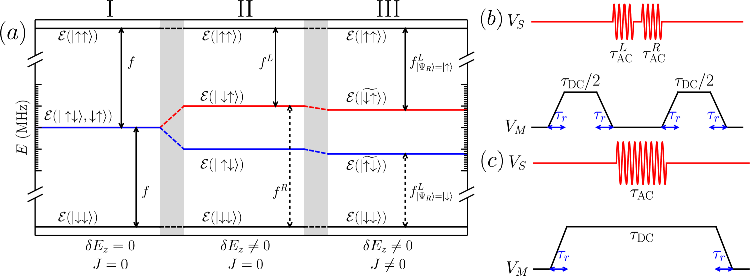
Figure 2: (a) Eigenenergies $\mathcal{E}$ of two spins in a double quantum dot in the presence of a magnetic field gradient and relevant transitions between them for three distinct realistic Zajac et al. parameter regimes. Regime I describes the case without a magnetic field gradient in which all single-spin flip transitions are energetically degenerate. In the presence of a field gradient (Regime II) the degeneracy of the transition frequencies between the left (solid-line arrow) and right spin (dashed-line arrow) is lifted, making it possible to energetically distinguish between single-qubit operations on the left and right spin. Turning on the exchange interaction, $J\ll\delta E_{z}$, (Regime III) further distinguishes conditional spin-flips from each other, i.e. the left ESR resonance frequency now depends on the right spin state, thus, allowing for frequency-selective entangling two-qubit gates. Conditional spin flip operations are possible: e.g., resonantly driving the transition $\ket{\uparrow\uparrow}\leftrightarrow\ket{\widetilde{\downarrow\uparrow}}$ yields a single-shot CNOT gate. Since the eigenstates $\mathcal{E}(\ket{\widetilde{\downarrow\uparrow}}$) and $\mathcal{E}(\ket{\widetilde{\uparrow\downarrow}}$) are both energetically lowered (by $J/2$ for $J\ll\delta E_{z}$) the transition $\ket{\downarrow\downarrow}\leftrightarrow\ket{\widetilde{\uparrow\downarrow}}$ is detuned from resonance by $\sim J$. (b) Schematic pulse sequence of the spin-echo CPHASE gate described in subsection III.1. Two adiabatic middle barrier pulses of length $\tau_{\text{DC}}/2$ and ramp length $\tau_{r}$ are combined with two ac pulses of length $\tau_{\text{AC}}^{L,R}$, performing a spin-flip on the left and right spin. (c) Schematic pulse sequence of the frequency selective CNOT gate. An adiabatic middle barrier pulse with length $\tau_{\text{DC}}$ and ramp length $\tau_{r}$ is combined with an ac pulse of length $\tau_{\text{AC}}$ resulting in a conditional spin-flip.

III DC Entangling gates: Strong and weak exchange

Two-qubit gates between neighboring single-spin qubits are realizable using the exchange interaction between the spins Loss and DiVincenzo (1998); Petta et al. (2005) with or without a magnetic field gradient Burkard et al. (1999b); Meunier et al. (2011). If the exchange energy dominates the Hamiltonian (3), i.e. $J\gg\delta E_{z}$, the (approximate) two-qubit eigenstates are the spin singlet, $\ket{\uparrow\downarrow}-\ket{\downarrow\uparrow}$ and triplets, $\ket{\uparrow\uparrow}$, $\ket{\uparrow\downarrow}+\ket{\downarrow\uparrow}$, $\ket{\downarrow\downarrow}$, and the resulting operation yields (for $\delta E_{z}=0$) the entangling $\sqrt{\text{SWAP}}$-gate. Sequential implementation of two $\sqrt{\text{SWAP}}$-gates and single-qubit rotations yields a CNOT-gate Loss and DiVincenzo (1998). In the case of weak exchange, i.e. $J\ll\delta E_{z}$, the two-qubit states are effectively the product states $\ket{\uparrow\uparrow}$, $\ket{\widetilde{\uparrow\downarrow}}$, $\ket{\widetilde{\downarrow\uparrow}}$, $\ket{\downarrow\downarrow}$ with small corrections in $\ket{\widetilde{\uparrow\downarrow}}$ and $\ket{\widetilde{\downarrow\uparrow}}$ due to spin-charge hybridization. In this limit the exchange interaction yields a conditional phase (CPHASE) gate. In this paper we focus on the regime $J\ll\delta E_{z}$ which is typical for DQD systems in the presence of a micromagnet. However, for adiabatic pulses, with ramp time $\tau_{r}\gg J/\delta E_{z}^{2}$, both implementations are equivalent. Note, that the criteria for the adiabatic regime is usually fulfilled in state-of-the-art devicesZajac et al. ; Yoneda et al. ; Watson et al. . For an adiabatic pulse the instantaneous eigenvalues of the Hamiltonian (3) are given as follows;

$$\mathcal{E}(\ket{\uparrow\uparrow}) =E_{z},$$ (4)

$$\mathcal{E}(\ket{\widetilde{\uparrow\downarrow}}) =\left(-J-\sqrt{J^{2}+\delta E_{z}^{2}}\right)/2,$$ (5)

$$\mathcal{E}(\ket{\widetilde{\downarrow\uparrow}}) =\left(-J+\sqrt{J^{2}+\delta E_{z}^{2}}\right)/2,$$ (6)

$$\mathcal{E}(\ket{\downarrow\downarrow}) =-E_{z}.$$ (7)

Figure 2 (a) shows the eigenenergies for three different parameter regimes for $J\ll\delta E_{z}$. Note, that for $J\ll\delta E_{z}$ one can use the expansion $\sqrt{J^{2}+\delta E_{z}^{2}}\approx\delta E_{z}+\frac{J^{2}}{2\delta E_{z}}$ simplifying the expressions in Eqs. (5) and (6). The time evolution of an adiabatic exchange pulse of length $\tau$ in the rotating frame $\widetilde{H}(t)=R^{\dagger}HR+\mathrm{i}\dot{R}^{\dagger}R$ with $R=\exp\left[-\mathrm{i}\omega t(S_{z,L}+S_{z,R})/\hbar\right]$ and $\hbar\omega=E_{z}/2$ is given by

$$U(\tau)=\text{diag}\left[1,\,\,\mathrm{e}^{\mathrm{i}\left(J+\sqrt{J^{2}+\delta E_{z}^{2}}\right)\frac{\tau}{2\hbar}},\,\,\mathrm{e}^{\mathrm{i}\left(J-\sqrt{J^{2}+\delta E_{z}^{2}}\right)\frac{\tau}{2\hbar}},1\right].$$ (8)

Note that here $g(J)\tau$, for arbitrary functions $g$, is defined as $g(J)\tau\equiv\int_{0}^{\tau}g(J(t))dt$. The time evolution up to a global phase can be decomposed into two parts as $U=U_{\text{ent}}U_{\text{loc}}$ with an entangling term

$$U(\tau)_{\text{ent}}=\exp\left(\mathrm{i}J\tau\,S_{z,L}S_{z,R}/\hbar\right)$$ (9)

and an accumulated local phase

$$U(\tau)_{\text{loc}}= \exp\left(-\mathrm{i}\sqrt{J^{2}+\delta E_{z}^{2}}(S_{z,L}-S_{z,R})\tau/\hbar\right)$$

$$\approx \exp\left[-\mathrm{i}\left(\delta E_{z}+\frac{J^{2}}{2\delta E_{z}}\right)(S_{z,L}-S_{z,R})\tau/\hbar\right].$$ (10)

For gate times being odd integer multiples of $\hbar\pi/J$, $\tau=(2n+1)\hbar\pi/J$ and the time-evolution (9) is equivalent to CPHASE up to single-qubit $z$-rotations Meunier et al. (2011). Even multiples, $\tau_{\text{DC}}\equiv\tau=2\hbar\pi n/J$, correspondingly yield identity up to local $S_{z}$-rotations $\mathrm{e}^{\mathrm{i}\Phi_{L}S_{z,L}/2}$ and $\mathrm{e}^{\mathrm{i}\Phi_{R}S_{z,R}/2}$ for the left and right spin. From Eq. (10) we find the following expressions for the phases,

$$\Phi_{L}^{\text{DC}} =-2\pi n\sqrt{J^{2}+\delta E_{z}^{2}}/J,$$ (11)

$$\Phi_{R}^{\text{DC}} =2\pi n\sqrt{J^{2}+\delta E_{z}^{2}}/J.$$ (12)

The correction of these phases will be discussed in subsection IV.1. The fact that the dc CPHASE operation can be cancelled out will be important for the ac gate discussed in section IV.

III.1 High fidelity dc implementation

In the experimental configuration described above, the magnetic gradient can exceed the nominal exchange splitting due to residual tunneling to a high degree. Thus we can examine the type of gates that may provide high fidelity operation in that environment. We assume that in the case of a nominal zero induced exchange, the two spin system is described by a Hamiltonian

$$H_{0}=E_{z}(S_{z,L}+S_{z,R})+\delta E_{z}(S_{z,L}-S_{z,R})/2$$ (13)

where we used the same definitions as above. We have neglected the transverse magnetic gradient which causes individual spin flips and is suppressed by the Zeeman energy $E_{z}$. We also neglect the induced double-spin flip transitions by the diagonalization of the physical Hamiltonian under finite residual exchange $J_{0}$.

We consider the inclusion of an echo mechanism for removing the excess phase terms in the exchange gate as well as potential unknown magnetic gradients. In order to examine the spin parity subspaces efficiently, we define new Pauli matrices, $\sigma_{x}=S_{+,L}S_{-,R}+{H.c.}$, $\sigma_{z}=S_{z,L}-S_{z,R}$, and the projector $P=(1-4S_{z,L}S_{z,R})/2$, acting only in the odd parity space. In a similar manner, we define $\tau_{z}=S_{z,L}+S_{z,R}$ and $\tau_{x}=S_{+,L}S_{+,R}+S_{-,L}S_{-,R}$. In this basis, the (time-dependent) Hamiltonian (1) neglecting transverse gradient fields is

$$H(t)=E_{z}\tau_{z}+\delta E_{z}\sigma_{z}/2-J(t)[P-\sigma_{x}]/2$$ (14)

with $J(t)$ being the ramp-induced exchange. We also note that a $\pi$ pulse on both spins about the $x$-axis corresponds, up to a global phase, to the unitary $\tau_{x}+\sigma_{x}$ while a pair of $y$-axis pulses would correspond to $\tau_{x}-\sigma_{x}$.

For both fast and slow exchange pulses of length $T$, we see that the even parity space only undergoes evolution according to $E_{z}\tau_{z}$, and thus will effectively factor out after inclusion of the $\pi$ pulses shown in Fig. 2 (b). Meanwhile, the odd parity space undergoes nontrivial evolution, due to both the overall phase evolution $-\int_{0}^{T}Jdt/2$ and from the rotations in the subspace about the axis $(J,0,\delta E_{z})$.

We first consider fast instantaneous changes of $J$. The time evolution is then stroboscopically given by rotations for a controlled period about various axes in the odd parity ($P$) subspace. A simple exchange pulse corresponds to

$$U_{J}= (\mathbb{I}-P)\mathrm{e}^{-\mathrm{i}TE_{z}\tau_{z}}+$$ (15)

$$\ \ P\mathrm{e}^{\mathrm{i}\Phi_{x}}\left[\cos(\Omega_{J}T)-\mathrm{i}\frac{J\sigma_{x}+\delta E_{z}\sigma_{z}}{2\Omega_{J}}\sin(\Omega_{J}T)\right]$$

with $\Omega_{J}=\sqrt{\delta E_{z}^{2}+J^{2}}/2$ and $\Phi_{x}=\int_{0}^{T}Jdt/2=JT/2$. We note that for $\Omega_{J}T=n\pi$ with integer $n$, we obtain a CPHASE gate with phase $\Phi_{x}=\frac{J}{\sqrt{\delta E_{z}^{2}+J^{2}}}n\pi$, as the $\sin$ terms vanishes, which presents one way to remove the excess phase.

We now add the additional rotations of individual spins in the middle of the sequence. Towards this end, we would like to understand how this gate behaves in the rotating frame in which we apply our single qubit gates. Note that in this subsection, our rotating frame has a different frequency for each of the two spins, representing the frequencies of the local oscillators used to drive individual spin resonance (motivated by experiment Zajac et al. ). If we envision starting $U_{J}$ at time $t_{1}$ and ending it at time $t_{2}=t_{1}+T$, we need to know the rotating frame state at the end of the sequence. We can move $U_{J}$ to this rotating frame, $R=\mathrm{e}^{-\mathrm{i}(\omega_{1}S_{z,L}+\omega_{2}S_{z,R})t}$, defined by the qubit frequencies $\omega_{1}=(E_{z}+\delta E_{z}/2)/\hbar$ and $\omega_{2}=(E_{z}-\delta E_{z}/2)/\hbar$ and applying the unitary transformation $\ket{\psi_{\text{rf}}(t)}=R^{\dagger}\ket{\psi_{\text{lab}}(t)}$. Thus, we have

$$\ket{\psi_{\text{rf}}(t_{2})}=R^{\dagger}U_{J}R\ket{\psi_{\text{rf}}(t_{1})}=U_{J}^{\text{rf}}(t_{2},t_{1})\ket{\psi_{\text{rf}}(t_{1})},$$ (16)

where we move back to the lab frame, apply $U_{J}$, then move back to the rotating frame.

In total, in the rotating frame, we find

$$U_{J}^{\text{rf}}(t_{1}+T,t_{1}) =(\mathbb{I}-P)+P\mathrm{e}^{\mathrm{i}\Phi_{x}}\mathrm{e}^{\mathrm{i}\delta E_{z}T\sigma_{z}/4}\left[\cos(\Omega_{J}T)-\mathrm{i}\frac{J\sigma_{\mu}+\delta E_{z}\sigma_{z}}{2\Omega_{J}}\sin(\Omega_{J}T)\right]\mathrm{e}^{\mathrm{i}\delta E_{z}T\sigma_{z}/4}$$ (17)

where $\sigma_{\mu}=\cos(\delta E_{z}(2t_{1}+T)/2)\sigma_{x}+\sin(\delta E_{z}(2t_{1}+T)/2)\sigma_{y}$. Thus the wait time $t_{1}$ enters in the definition of the rotation axis. While we do not necessarily want any such rotation, as the diagonal term $\sim J$ will perform a CPHASE-like evolution, we will have to be careful to make certain effects from this are removed.

One approach for removing the flip-flop effect consists in moving adiabatically with respect to $\delta E_{z}$. Diagonalization of $H(t)$ in the rotating frame yields $\tilde{H}^{\text{rf}}=-PJ(t)/2+(\Omega_{J}(t)-\delta E_{z}/2)\sigma_{z}$ with $\Omega_{J}(t)=\sqrt{\delta E_{z}^{2}+J(t)^{2}}/2$. Small non-adiabatic corrections enter with a $\sigma_{+}$ term, which behave in a similar manner to the $\sigma_{x}$ term given by $U_{J}$ for the fast case. The net result of the adiabatic case in the rotating frame is

$$U_{\text{ad}}^{\text{rf}}=(1-P)+P\mathrm{e}^{\mathrm{i}\Phi_{\text{ad}}}\mathrm{e}^{-\mathrm{i}\sigma_{z}\phi_{z}}$$ (18)

with $\Phi_{\text{ad}}=\int_{0}^{T}J(t)dt/2$ and $\phi_{z}=\int_{0}^{T}\sqrt{\delta E_{z}^{2}+J(t)^{2}}dt/2-\delta E_{z}T/2$. Thus we see that the adiabatic $J$ pulse leads to an extra single qubit $z$ rotation for both spins, in addition to the desired CPHASE-like operation. Note, that this phase in the rotating frame of the individual spins is equivalent to the phase given by Eqs. (11) and (12) for $n=1$.

We now consider a more general solution to the extra phase evolution (corresponding to a potentially undesired set of single qubit $z$ rotations) as well as the extra rotation about the $\mu$-axis. Specifically, we consider two $\pi$ pulses about the $x$-axis on the qubits in between two CPHASE-like unitaries (see Fig. 2 (b)). For the adiabatic case, we have

$$U_{c,\text{ad}} =U^{\text{rf}}_{\text{ad}}(4S_{x,L}S_{x,R})U^{\text{rf}}_{\text{ad}}$$ (19)

$$=(4S_{x,L}S_{x,R})\left[(1-P)+P\mathrm{e}^{\mathrm{i}\Phi_{\text{ad}}}\mathrm{e}^{\mathrm{i}\sigma_{z}\phi_{z}}\right]$$

$$\ \ \times\left[(1-P)+P\mathrm{e}^{\mathrm{i}\Phi_{\text{ad}}}\mathrm{e}^{-\mathrm{i}\sigma_{z}\phi_{z}}\right]$$ (20)

$$=(4S_{x,L}S_{x,R})\left[(1-P)+P\mathrm{e}^{2\mathrm{i}\Phi_{\text{ad}}}\right]$$ (21)

$$=4S_{x,L}S_{x,R}\mathrm{e}^{-2\mathrm{i}\Phi_{\text{ad}}(S_{z,L}+S_{z,R})}U_{\rm CPHASE},$$ (22)

where $U_{\rm CPHASE}=\textrm{diag}[1,1,1,\mathrm{e}^{-2\mathrm{i}\Phi_{\text{ad}}}]$. For the special case of $2\Phi_{\text{ad}}=\pi$, we find for our gate

$$U_{\pi,\text{ad}}=(4S_{y,L}S_{y,R})U_{\text{CZ}}.$$ (23)

Returning to the fast pulse version of the gate, Eq. (17), we see that the same $\pi$ pulses in the middle lead to

$$U_{c,\text{fast}} =U_{J}^{\text{rf}}(t_{2}+T,t_{2})(4S_{x,L}S_{x,R})U_{J}^{\text{rf}}(T,0)$$ (24)

$$=U_{J}^{\text{rf}}(t_{2}+T,t_{2})(\tau_{x}+\sigma_{x})U_{J}^{\text{rf}}(T,0)$$ (25)

$$=(\mathbb{I}-P)\tau_{x}+P\mathrm{e}^{2\mathrm{i}\Phi_{x}}\mathrm{e}^{\mathrm{i}\delta E_{z}(t_{2}+T)\sigma_{z}/2}\left[c-\vec{n}\cdot\vec{\sigma}s\right]$$

$$\ \ \times\mathrm{e}^{-\mathrm{i}\delta E_{z}t_{2}\sigma_{z}/2}\sigma_{x}\mathrm{e}^{\mathrm{i}\delta E_{z}T\sigma_{z}/2}\left[c-\vec{n}\cdot\vec{\sigma}s\right]$$ (26)

where $c=\cos(\Omega_{J}T)$, $s=\sin(\Omega_{J}T)$, $\vec{n}=(J,0,\delta E_{z})/(2\Omega_{J})$. In order to remove the terms proportional to $\vec{n}$ in the above, we need the action of the intermediate rotation $\mathrm{e}^{-\mathrm{i}\delta E_{z}t_{2}\sigma_{z}/2}\sigma_{x}\mathrm{e}^{\mathrm{i}\delta E_{z}T\sigma_{z}/2}$ to correspond to $\sigma_{y}$. That requires $\sin(\delta E_{z}(t_{2}+T)/2)=\pm 1$.

Furthermore, we want the equivalent unitary after the sequence,

$$\mathrm{e}^{\mathrm{i}\delta E_{z}/2(t_{2}+T)\sigma_{z}}\sigma_{y}$$

to be $\sigma_{x}$, which in turn requires $\delta E_{z}(t_{2}+T)/2=(2n+1)\pi$ with integer $n$. Conveniently, these are the same requirement.

IV Resonant single step CNOT gate

Additional controllability is given if the adiabatic dc exchange pulse is combined with microwave ac driving, $B_{y}^{Q}(t)\propto\cos(\omega t+\varphi)$, matching the transition frequencies between the two-qubit states which allows for direct conditional spin-flips. The gate sequence is outlined in Fig. 2 (b) and the basic concept is visualized in Fig. 2 (a) regime III. With the exchange interaction turned on the energy of both eigenstates $\ket{\widetilde{\uparrow\downarrow}}$ and $\ket{\widetilde{\downarrow\uparrow}}$ is lowered by $\sim J/2$, providing in total six energetically distinct resonance frequencies in the spectrum. There are four entangling transitions corresponding to the four conditional spin-flips. For example, inducing a resonant spin-flip between the states $\ket{\uparrow\uparrow}\leftrightarrow\ket{\widetilde{\downarrow\uparrow}}$ yields a CNOT with the right qubit as control and the left qubit as target gate as the following truth-table shows

$$\begin{split}\ket{\uparrow\uparrow}&\rightarrow\ket{\downarrow\uparrow}\\ \ket{\uparrow\downarrow}&\rightarrow\ket{\uparrow\downarrow}\\ \ket{\downarrow\uparrow}&\rightarrow\ket{\uparrow\uparrow}\\ \ket{\downarrow\downarrow}&\rightarrow\ket{\downarrow\downarrow}.\end{split}$$ (27)

In the remainder of this article, we always refer to this implementation of CNOT, however, in experiments other transitions can be resonantly driven as well, giving access to a much larger set of two-qubit quantum gates.

From the eigenenergies (4)-(7) the corresponding resonance frequencies of the four conditional transitions are given as follows;

$$f^{L}_{\ket{\Psi_{R}}=\ket{\downarrow}}\equiv |\mathcal{E}(\ket{\downarrow\downarrow})-\mathcal{E}(\ket{\widetilde{\uparrow\downarrow}})|$$

$$= E_{z}+\left(-J-\sqrt{J^{2}+\delta E_{z}^{2}}\right)/2,$$ (28)

$$f^{L}_{\ket{\Psi_{R}}=\ket{\uparrow}}\equiv |\mathcal{E}(\ket{\widetilde{\downarrow\uparrow}})-\mathcal{E}(\ket{\uparrow\uparrow})|$$

$$= E_{z}+\left(J-\sqrt{J^{2}+\delta E_{z}^{2}}\right)/2,$$ (29)

$$f^{R}_{\ket{\Psi_{L}}=\ket{\downarrow}}\equiv |\mathcal{E}(\ket{\downarrow\downarrow})-\mathcal{E}(\ket{\widetilde{\downarrow\uparrow}})|$$

$$= E_{z}+\left(-J+\sqrt{J^{2}+\delta E_{z}^{2}}\right)/2,$$ (30)

$$f^{R}_{\ket{\Psi_{L}}=\ket{\uparrow}}\equiv |\mathcal{E}(\ket{\widetilde{\uparrow\downarrow}})-\mathcal{E}(\ket{\uparrow\uparrow})|$$

$$= E_{z}+\left(J+\sqrt{J^{2}+\delta E_{z}^{2}}\right)/2.$$ (31)

One important observation is that the splitting between the conditional spin-flips is always provided by exchange,

$$f^{L}_{\ket{\Psi_{R}}=\ket{\uparrow}}-f^{L}_{\ket{\Psi_{R}}=\ket{\downarrow}}=f^{R}_{\ket{\Psi_{L}}=\ket{\uparrow}}-f^{R}_{\ket{\Psi_{L}}=\ket{\downarrow}}=J.$$ (32)

IV.1 High fidelity ac implementation

We have shown so far that we can effectively cancel out the CPHASE gate from the dc dynamics of our frequency selective gate by appropriately timing the length of the dc exchange pulse $t_{\text{DC}}=2\pi n/J$ where $n$ is a positive integer. This can be thought of applying CPHASE twice (times $n$) which undo each other. However, there are two additional effects which will disturb the gate if not treated appropriately. The first effect results from the off-resonant driving of nearby transitions, which can be important if $J$ is comparable to the Rabi frequency, and a second effect originates from relative phase accumulation of the spins during the microwave drive. Below we discuss both effects and how they can be avoided.

In the experiment described in Ref. Zajac et al. the gates are driven at the resonance frequency $\omega=f^{L}_{\ket{\Psi_{R}}=\ket{\uparrow}}$ during a dc exchange pulse which flips the left spin if and only if the right spin is in the state $\ket{\Psi_{R}}=\ket{\uparrow}$ inducing a transition between the $\ket{\uparrow\uparrow}$ and $\ket{\widetilde{\downarrow\uparrow}}$ states. However, the energy separation of the transition frequency $f^{L}_{\ket{\Psi_{R}}=\ket{\uparrow}}$ and the transition frequency for an opposite right spin, $\ket{\Psi_{R}}=\ket{\downarrow}$, is given by the exchange interaction strength $J$ (see Eq. (32)). In the regime of operation  Zajac et al. $\delta E_{z}\gg J\approx 20\,\mathrm{MHz}$ the transition between the states $\ket{\uparrow\downarrow}$ and $\ket{\widetilde{\downarrow\downarrow}}$ is also driven and gives rise to off-resonant Rabi dynamics. Other transitions, $f^{R}_{\ket{\Psi_{L}}=\ket{\uparrow}}$ and $f^{R}_{\ket{\Psi_{L}}=\ket{\downarrow}}$, are even further off-resonant because they are separated in energy by $\delta E_{z}$, and will be neglected here.

Starting with the Hamiltonian (3) in the rotating frame $\widetilde{H}(t)=R^{\dagger}HR+\mathrm{i}\dot{R}^{\dagger}R$ with $R=\exp\left[-\mathrm{i}\omega t(S_{z,L}+S_{z,R})/\hbar\right]$ and neglecting fast oscillations, we find in the instantaneous adiabatic basis $\{\ket{\uparrow\uparrow},\ket{\widetilde{\downarrow\uparrow}},\ket{\widetilde{\uparrow\downarrow}},\ket{\downarrow\downarrow}\}$ for $J\ll\delta E_{z}$

$$\widetilde{H}(t)\approx\frac{1}{2}\left(\begin{matrix}2(E_{z}-\omega)&-\mathrm{i}\alpha_{1}^{*}&-\mathrm{i}\beta_{1}^{*}&0\\ \mathrm{i}\alpha_{1}&-J+(\delta E_{z}+\frac{J^{2}}{2\delta E_{z}})&0&-\mathrm{i}\beta_{2}^{*}\\ \mathrm{i}\beta_{1}&0&-J-(\delta E_{z}+\frac{J^{2}}{2\delta E_{z}})&-\mathrm{i}\alpha_{2}^{*}\\ 0&\mathrm{i}\beta_{2}&\mathrm{i}\alpha_{2}&-2(E_{z}-\omega)\\ \end{matrix}\right).$$ (33)

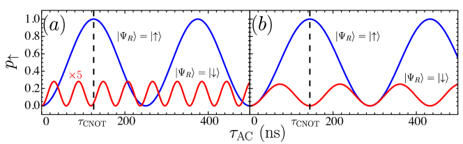
Figure 3: Schematic plot of the resonant (blue) and off-resonant (red) transition probabilities with (a) desynchronized and (b) synchronized Rabi frequencies $\Omega$ and $\widetilde{\Omega}$ (see Eq. (41)). A CNOT gate is provided at time $\tau_{\text{CNOT}}$ where the resonant driving exactly flips the spin for $\ket{\Psi_{R}}=\ket{\uparrow}$ (blue). (a) Using an arbitrary Rabi frequency $\Omega$, we find that the frequencies are desynchronized and the off-resonant driving also yields a finite population of the flipped spin for $\ket{\Psi_{R}}=\ket{\downarrow}$ (red). (b) Synchronized resonant Rabi frequency $\Omega$ and off-resonant Rabi frequency $\widetilde{\Omega}$ which avoids any undesired population for $\ket{\Psi_{R}}=\ket{\downarrow}$. We choose $m=0$ and $n=1$ for the fastest realization of the synchronized CNOT gate yielding an ac pulse length $\tau_{\text{AC}}\approx 94\,\mathrm{ns}$ using parameters from the experiment in Ref. Zajac et al. . Note that to enhance the visibility, we rescaled the off-resonant state probabilities in (a) by a factor of $5$.

Here $\alpha_{1,2}\approx[\pm B^{L,1}_{y}+B^{R,1}_{y}J/(2\delta E_{z})]\,\,\mathrm{e}^{\mathrm{i}\theta}$ and $\beta_{1,2}\approx[\mp B^{R,1}_{y}+B^{L,1}_{y}J/(2\delta E_{z})]\,\,\mathrm{e}^{\mathrm{i}\theta}$ are the effective microwave driving amplitudes after transforming into the adiabatic basis. Nearby the resonance frequency $\omega-\delta\omega=f^{L}_{\ket{\Psi_{R}}=\ket{\uparrow}}\approx E_{z}-\{\delta E_{z}+J[1-J/(2\delta E_{z})]\}/2$, $\beta_{1,2}\approx 0$, the Hamiltonian (33) decouples into two blocks, $\{\ket{\uparrow\uparrow},\ket{\widetilde{\downarrow\uparrow}}\}$ and $\{\ket{\widetilde{\uparrow\downarrow}},\ket{\downarrow\downarrow}\}$ which are separated in energy by $\sim\delta E_{z}$ (see Eq. (32)) and evolve independently in time. Therefore, we find in the basis $\{\ket{\uparrow\uparrow},\ket{\widetilde{\downarrow\uparrow}},\ket{\widetilde{\uparrow\downarrow}},\ket{\downarrow\downarrow}\}$

$$\widetilde{H}(t)\approx\frac{1}{2}\left(\begin{array}[]{cc|cc}-J+(\delta E_{z}+\frac{J^{2}}{2\delta E_{z}})-\delta\omega&-\mathrm{i}\alpha_{1}^{*}&0&0\\ \mathrm{i}\alpha_{1}&-J+(\delta E_{z}+\frac{J^{2}}{2\delta E_{z}})&0&0\\ \hline\cr 0&0&-J-(\delta E_{z}+\frac{J^{2}}{2\delta E_{z}})&-\mathrm{i}\alpha_{2}^{*}\\ 0&0&\mathrm{i}\alpha_{2}&J-(\delta E_{z}+\frac{J^{2}}{2\delta E_{z}})+\delta\omega\\ \end{array}\right).$$ (38)

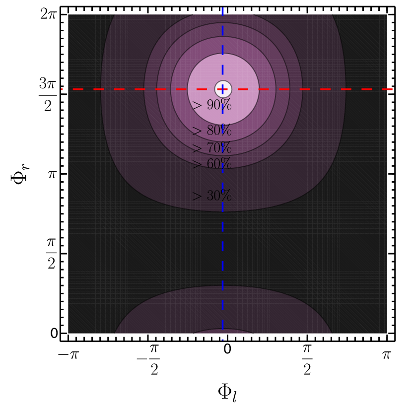
Figure 4: Simulated CNOT gate fidelity (in percent) as a function of the compensated phase $\Phi_{L}$ and $\Phi_{R}$ on the left spin (target) and right spin (control) after the ac drive. Compensation is provided for a $z$-Rotation $\hat{Z}(\Phi)$ on the left spin with $\Phi_{l}=2\pi k_{l}-\Phi_{L}$ and on the right spin $\Phi_{r}=2\pi k_{r}-\Phi_{R}$ with integers $k_{l}$ and $k_{r}$, thus $\Phi=(\Phi_{l},\Phi_{r})\approx(-0.03\pi,-0.469\pi)$ (blue and red dashed lines). For the simulation we used the following parameters related to the experiment in Ref. Zajac et al. ; $J=19.7\,\mathrm{MHz}$, $\delta E_{z}=210\,\mathrm{MHz}$, $\tau_{r}=5\,\mathrm{ns}$, $\tau_{\text{CNOT}}=94\,\mathrm{ns}$ (corresponding to $\alpha=1/(2\tau_{\text{CNOT}})$, $\tau_{\text{DC}}=198\,\mathrm{ns}$, and $m=0$ and $n=1$ in Eq. 41)

.

For $\delta\omega=0$, only $f^{L}_{\ket{\Psi_{R}}=\ket{\uparrow}}$ (top-left block) is resonant and yields full Rabi oscillations with a Rabi frequency $\Omega=|\alpha_{1}|/\hbar$ while $f^{L}_{\ket{\Psi_{R}}=\ket{\downarrow}}$ (bottom-right block) is detuned (off-resonant) by $J$, therefore, performing partial spin-flips with the detuned Rabi frequency $\widetilde{\Omega}=\sqrt{|\alpha_{2}|^{2}+J^{2}}/\hbar$. Since the time evolution of each $2\times 2$ block can be computed individually we find the following time evolutions of each block for $\theta=3\pi/2$,

$$U_{\ket{\Psi_{R}}=\ket{\uparrow}}=\mathrm{e}^{-\frac{\mathrm{i}tc_{1}}{2}} \left[\cos\left(\frac{\Omega t}{2}\right)\mathds{1}+\mathrm{i}\sin\left(\frac{\Omega t}{2}\right)\sigma_{x}\right],$$ (39)

$$U_{\ket{\Psi_{R}}=\ket{\downarrow}}=\mathrm{e}^{-\frac{\mathrm{i}tc_{2}}{2}} \left[\cos\left(\frac{\widetilde{\Omega}t}{2}\right)\mathds{1}+\mathrm{i}\sin\left(\frac{\widetilde{\Omega}t}{2}\right)\right.$$

$$\left.\times\left(\frac{|\alpha_{2}|}{2\,\hbar\,\widetilde{\Omega}}\sigma_{x}-\frac{J}{2\,\hbar\,\widetilde{\Omega}}\sigma_{z}\right)\right].$$ (40)

with the frequencies $\hbar c_{1}=-J+(\delta E_{z}+\frac{J^{2}}{2\delta E_{z}})$ and $\hbar c_{2}=-\delta E_{z}-\frac{J^{2}}{2\delta E_{z}}$. Setting $t=\pi\,(2m+1)/\Omega$ with integer $m$ yields a spin flip in the $\ket{\Psi_{R}}=\ket{\uparrow}$ block. In order to cancel the dynamics of the off-resonant states, we synchronize the Rabi frequencies by setting

$$\Omega=\frac{2m+1}{2n}\widetilde{\Omega},$$ (41)

with an integer $n$. This can be achieved by adjusting the ac driving strength $B^{L,1}_{y}$. Considering $B^{L,1}_{y}=B^{R,1}_{y}$, we find the following analytical result for the ac driving strength,

$$B^{L,1}_{y}=a_{n,m}\equiv\pm\frac{J}{\sqrt{\frac{4n^{2}}{(2m+1)^{2}}\left(1+\frac{J}{2\delta E_{z}}\right)^{2}-\left(1-\frac{J}{2\delta E_{z}}\right)^{2}}},$$ (42)

with integer $m$ and $n$ which fulfills Eq. (41). A comparison of the dynamics with and without synchronization is given in Fig. 3.

The second effect we observe is a phase accumulation for each individual spin during the microwave drive. During the CNOT gate a dynamic phase is acquired on the right (control) spin originating from the energy difference between the two blocks in Eq. (38). While $\ket{\Psi_{R}}=\ket{\uparrow}$ states are oscillating with $\mathrm{e}^{-\frac{\mathrm{i}tc_{1}}{2}}$, $\ket{\Psi_{R}}=\ket{\downarrow}$ states oscillate with $\mathrm{e}^{-\frac{\mathrm{i}tc_{2}}{2}}$ which yields a relative phase after the ac spin flip, $\Phi_{R}\propto(c_{1}-c_{2})\tau_{\text{AC}}$, on the right spin (see Eqs. (39) and (40)). Additionally, we observe a holonomic phase Sjöqvist (2016) on the right spin which results from Rabi’s equation for a full (half) cycle and can directly be seen in Eqs. (39) and (40) whether $\cos(\cdot)$ ($\sin(\cdot)$) becomes positive or negative depending on the choice of $m$ and $n$. We find the following analytic expressions for the phase difference on the right (control) spin after the ac spin flip,

$$\Phi_{R}^{\text{AC}}=-\pi \left[\left(m-n+\frac{1}{2}\right)\phantom{\frac{2m+1}{a_{n,m}\left(1+\frac{J}{2\delta E_{z}}\right)}}\right.$$

$$\left.-\frac{2m+1}{a_{n,m}\left(1+\frac{J}{2\delta E_{z}}\right)}\left(\delta E_{z}+\frac{J^{2}}{\delta E_{z}}-\frac{J}{2}\right)\right].$$ (43)

In order to find the phase accumulated during the full CNOT gate, consisting of dc pulse and ac pulse, the ac phase error, Eq. (43) and the dc phase error, Eqs. (11) and (12), have to be combined. Considering the rotating frames for the dc and ac phase accumulation, we find the following results in the rotating frame of each individual spin, $R=\exp\left[-\mathrm{i}t(\omega_{1}S_{z,L}+\omega_{2}S_{z,R})/\hbar\right]$, with $\omega_{1}=(E_{z}+\delta E_{z}/2)/\hbar$ and $\omega_{2}=(E_{z}-\delta E_{z}/2)/\hbar$ (motivated by experiment Zajac et al. );

$$\Phi_{L} =\Phi_{L}^{\text{DC}}+\frac{\delta E_{z}}{2}\tau_{\text{DC}}+\frac{\sqrt{\delta E_{z}^{2}+J^{2}}}{2}\tau_{\text{AC}},$$ (44)

$$\Phi_{R} =\Phi_{R}^{\text{DC}}-\frac{\delta E_{z}}{2}\tau_{\text{DC}}+\Phi_{R}^{\text{AC}}-\frac{\sqrt{\delta E_{z}^{2}+J^{2}}}{2}\tau_{\text{AC}}.$$ (45)

This additional phase can either be compensated by adjusting $J$ such that the phase is a multiple of $2\pi$ (not possible in our regime of operation) or including an additional $z$-rotation directly after the CNOT gate with angles $\Phi_{l}=2k_{1}\pi-\Phi_{L}$ and $\Phi_{r}=2k_{2}\pi-\Phi_{R}$ with integers $k_{1,2}$. Simulations where we numerically integrate the time-dependent Schrödinger equation $i\hbar\dot{\Psi}(t)=\widetilde{H}(t)\Psi(t)$ support our analysis (see Fig. 4). The highest fidelity can indeed be found after correcting the described phase shift. At this point it is worth mentioning that $z$-rotations in the experiment in Ref. Zajac et al. and similar experiments  Yoneda et al. ; Watson et al. can be performed by modifying the reference phase for the individual spins. This can be done rapidly and accurately in software with no additional microwave control required.

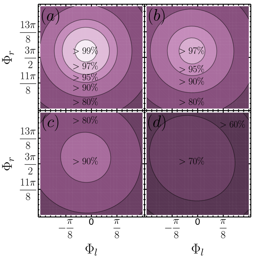
Figure 5: Zoom in of the simulation in Fig. 4 in the presence of charge noise fluctuations with strength (a) $\sigma_{\delta J}=0\,\mathrm{MHz}$, (b) $\sigma_{\delta J}=0.33\,\mathrm{MHz}$, (c) $\sigma_{\delta J}=0.67\,\mathrm{MHz}$, and (d) $\sigma_{\delta J}=1.33\,\mathrm{MHz}$. For the simulation the fluctuations are assumed to be quasistatic and Gaussian distributed with standard deviation $\sigma_{\delta J}$ and mean $\langle\delta J\rangle\approx 0$.

IV.2 Charge noise analysis

In semiconductor devices charge noise is omnipresentPaladino et al. (2014). In the simplest model, charge noise can be described as fluctuations of the electric potentials near the dot. Thus, charge noise couples to the two-qubit systems mainly through the exchange interactions due to its dependence on the detuning, tunneling, and confinement of the spins Burkard et al. (1999a); Das Sarma et al. (2011). To be precise, charge noise couples also to single spins through the same mechanism that allows EDSR to rotate the spin though fluctuations of the electron positions. This effect, however, is small as evidenced by Ref. Yoneda et al. , thus will be neglected in the analysis below.

In lowest order $J\rightarrow J+\delta J$ where $\delta J$ are fluctuations of the exchange energy due to charge noise, we find the following first-order corrections to the diagonal Hamiltonian (4)-(7) in the adiabatic basis $\{\ket{\uparrow\uparrow},\ket{\widetilde{\downarrow\uparrow}},\ket{\widetilde{\uparrow\downarrow}},\ket{\downarrow\downarrow}\}$

$$H_{\text{noise}}=\frac{2J\delta J}{\delta E_{z}}(\widetilde{S}_{z}^{L}+\widetilde{S}_{z}^{R})-2\delta J\widetilde{S}_{z}^{L}\widetilde{S}_{z}^{R}.$$ (46)

The first term induces single-qubit dephasing but is highly suppressed in the case of $J\ll\delta E_{z}$ since it has strength $\propto J/\delta E_{z}$. Therefore, large magnetic field gradients are beneficial for operating the two-qubit gate. The second term couples longitudinally to the two-qubit gate operation since it has the same form as the dc pulse, $\propto S_{z}^{L}S_{z}^{R}$, and reduces the fidelity of the resulting two-qubit gate that only depends on the bare charge noise fluctuations $\delta J$. In experiments Watson et al. , this is the limiting factor for the gate fidelity, since simple echo protocols which also filter out the desired two-qubit interaction would not work. Simulations assuming quasistatic noise show that for $\sigma_{\delta J}\equiv\sqrt{\langle\delta J^{2}\rangle-\langle\delta J\rangle^{2}}=0.33\,\mathrm{MHz}$ two-qubit gate fidelities $>97\%$ are still possible (see Fig. 5 (b)). However, fluctuations twice (four times) as large already limit the gate fidelity to about $\approx 93\%$ ($\approx 77\%$) (see Fig. 5 (c) and (d)), problematic for longer quantum algorithms. Mitigation of these effects is still possible through advanced pulse shaping or composite pulse sequences Vandersypen and Chuang (2005), complex dynamical decoupling sequences De and Pryadko (2014), and reduction of the amplitude of the fluctuations, i.e., operating at a charge noise sweet spot. Also, a partial recovery of the fidelity is still achieved as the conditional spin flip during the frequency selective CNOT gate serves as a simple spin-echo sequence, decoupling the left spin and low-frequency charge noise if $\ket{\Psi_{R}}=\ket{\uparrow}$. This can be seen by approximating the CNOT gate as follows Vandersypen and Chuang (2005);

$$U_{\text{CNOT}} =\mathrm{e}^{-\mathrm{i}(H_{\text{rf}}+H_{J})\tau_{\text{CNOT}}/\hbar}$$ (47)

$$\approx\mathrm{e}^{-\mathrm{i}H_{J}\,\tau/\hbar}\,\,\underbrace{\mathrm{e}^{-\mathrm{i}H_{\text{rf}}\,\tau/\hbar}}_{\text{CNOT}}\,\,\mathrm{e}^{-\mathrm{i}H_{J}\,\tau/\hbar}$$ (48)

with $\tau$ yet to be chosen. Here, the Hamiltonian $H_{\text{rf}}$ only contains ac driving and the Hamiltonian $H_{J}$ contains the dc exchange interaction, thus, fluctuations due to charge noise. Assuming an ideal CNOT gate, only entries in Eq. (48) corresponding to $\ket{\Psi_{R}}=\ket{\downarrow}$ contain $J+\delta J$, therefore, are affected by charge noise. Mathematically speaking, the time evolution $U_{\text{CNOT}}$ only affects density matrix elements corresponding to $\ket{\Psi_{R}}=\ket{\downarrow}$ states which dephase with characteristic time $T^{-1}_{\phi}\approx\left\langle\delta J(t)^{2}\right\rangle$, while density matrix elements only consisting of $\ket{\Psi_{R}}=\ket{\uparrow}$ states are protected. In average, this will lead to a reduced influence of noise. Hypothetically, the larger variety of two-qubit quantum gates (modulating different transitions) and the partial intrinsic spin-echo can be used to construct more efficient charge noise decoupling sequences.

V Conclusion

In this paper, we have presented high-fidelity implementations of a dc-pulsed CPHASE gate and a single-shot two-qubit CNOT gate.

For the dc-pulsed CPHASE gate, we have provided a high-fidelity implementation using dc exchange pulses. We have analyzed two regimes for the exchange pulses, slow (adiabatic) and fast (instantaneous) exchange pulses, and have described how to compensate for residual spin-flip and phase errors. In the adiabatic regime, spin-flip errors are suppressed by the magnetic field difference and we have identified the phases which the individual spins accumulate during the two-qubit operation. By intersecting the CPHASE gate by single-qubit spin-flips to form a spin-echo sequence, spin-flip errors and local phases which the individual spins acquired during the CPHASE gate, can be avoided even for the non-adiabatic exchange pulses.

For the ac single-shot two-qubit CNOT gate, we have presented a high-fidelity implementation through frequency-selective resonant modulations of the two-qubit transitions. By selecting different transition frequencies a larger set of two-qubit quantum gates is accessible allowing for more efficient algorithms. We are able to compensate all intrinsic errors due to off-resonant transitions by fine-tuning the ac driving amplitude such that the resonant and the off-resonant oscillations are synchronized. Additionally, we have identified phases which the individual spins accumulate during the two-qubit operation. These phases can be compensated for by performing single-qubit $z$-rotations after each CNOT gate. Our two-qubit gate implementation also incorporates a reduction of charge noise by suppression through large magnetic field gradients and a partial intrinsic spin-echo decoupling sequence. Using the synchronization technique and the analytic values of the accumulated phases, existing experiments are able to reach higher two-qubit gate fidelities exceeding $97\%$ under realistic assumptions. This opens the path to large-scale quantum computation previously limited by low-fidelity two-qubit gates.

- (1) D. M. Zajac, A. J. Sigillito, M. Russ, F. Borjans, J. M. Taylor, G. Burkard, and J. R. Petta, arXiv:1708.03530 .
- Loss and DiVincenzo (1998) D. Loss and D. P. DiVincenzo, Phys. Rev. A 57, 120 (1998).
- Zwanenburg et al. (2013) F. A. Zwanenburg, A. S. Dzurak, A. Morello, M. Y. Simmons, L. C. L. Hollenberg, G. Klimeck, S. Rogge, S. N. Coppersmith, and M. A. Eriksson, Rev. Mod. Phys. 85, 961 (2013).
- Steger et al. (2012) M. Steger, K. Saeedi, M. L. W. Thewalt, J. J. L. Morton, H. Riemann, N. V. Abrosimov, P. Becker, and H. J. Pohl, Science 336, 1280 (2012).
- Tyryshkin et al. (2012) A. M. Tyryshkin, S. Tojo, J. J. L. Morton, H. Riemann, N. V. Abrosimov, P. Becker, H.-J. Pohl, T. Schenkel, M. L. W. Thewalt, K. M. Itoh, and S. A. Lyon, Nat Mater 11, 143 (2012).
- Veldhorst et al. (2014) M. Veldhorst, J. C. C. Hwang, C. H. Yang, A. W. Leenstra, B. de Ronde, J. P. Dehollain, J. T. Muhonen, F. E. Hudson, K. M. Itoh, A. Morello, and A. S. Dzurak, Nat Nano 9, 981 (2014).
- Veldhorst et al. (2015) M. Veldhorst, C. H. Yang, J. C. C. Hwang, W. Huang, J. P. Dehollain, J. T. Muhonen, S. Simmons, A. Laucht, F. E. Hudson, K. M. Itoh, A. Morello, and A. S. Dzurak, Nature 526, 410 (2015).
- Takeda et al. (2016) K. Takeda, J. Kamioka, T. Otsuka, J. Yoneda, T. Nakajima, M. R. Delbecq, S. Amaha, G. Allison, T. Kodera, S. Oda, and S. Tarucha, Sci Adv 2, e1600694 (2016).
- (9) T. F. Watson, S. G. J. Philips, E. Kawakami, D. R. Ward, P. Scarlino, M. Veldhorst, D. E. Savage, M. G. Lagally, M. Friesen, S. N. Coppersmith, M. A. Eriksson, and L. M. K. Vandersypen, arXiv:1708.04214 .
- (10) J. Yoneda, K. Takeda, T. Otsuka, T. Nakajima, M. R. Delbecq, G. Allison, T. Honda, T. Kodera, S. Oda, Y. Hoshi, N. Usami, K. M. Itoh, and S. Tarucha, arXiv:1708.01454 .
- Lidar and Brun (2013) D. Lidar and T. Brun, Quantum Error Correction (Cambridge University Press, 2013).
- Brunner et al. (2011) R. Brunner, Y.-S. Shin, T. Obata, M. Pioro-Ladrière, T. Kubo, K. Yoshida, T. Taniyama, Y. Tokura, and S. Tarucha, Phys. Rev. Lett. 107, 146801 (2011).
- Zajac et al. (2016) D. M. Zajac, T. M. Hazard, X. Mi, E. Nielsen, and J. R. Petta, Phys. Rev. Applied 6, 054013 (2016).
- Pioro-Ladriere et al. (2008) M. Pioro-Ladriere, T. Obata, Y. Tokura, Y. S. Shin, T. Kubo, K. Yoshida, T. Taniyama, and S. Tarucha, Nat Phys 4, 776 (2008).
- Otsuka et al. (2016) T. Otsuka, T. Nakajima, M. R. Delbecq, S. Amaha, J. Yoneda, K. Takeda, G. Allison, T. Ito, R. Sugawara, A. Noiri, A. Ludwig, A. D. Wieck, and S. Tarucha, Scientific Reports 6, 31820 (2016).
- Burkard et al. (1999a) G. Burkard, D. Loss, and D. P. DiVincenzo, Phys. Rev. B 59, 2070 (1999a).
- Das Sarma et al. (2011) S. Das Sarma, X. Wang, and S. Yang, Phys. Rev. B 83, 235314 (2011).
- Petta et al. (2005) J. R. Petta, A. C. Johnson, J. M. Taylor, E. A. Laird, A. Yacoby, M. D. Lukin, C. M. Marcus, M. P. Hanson, and A. C. Gossard, Science 309, 2180 (2005).
- Bertrand et al. (2015) B. Bertrand, H. Flentje, S. Takada, M. Yamamoto, S. Tarucha, A. Ludwig, A. D. Wieck, C. Bäuerle, and T. Meunier, Phys. Rev. Lett. 115, 096801 (2015).
- Martins et al. (2016) F. Martins, F. K. Malinowski, P. D. Nissen, E. Barnes, S. Fallahi, G. C. Gardner, M. J. Manfra, C. M. Marcus, and F. Kuemmeth, Phys. Rev. Lett. 116, 116801 (2016).
- Reed et al. (2016) M. D. Reed, B. M. Maune, R. W. Andrews, M. G. Borselli, K. Eng, M. P. Jura, A. A. Kiselev, T. D. Ladd, S. T. Merkel, I. Milosavljevic, E. J. Pritchett, M. T. Rakher, R. S. Ross, A. E. Schmitz, A. Smith, J. A. Wright, M. F. Gyure, and A. T. Hunter, Phys. Rev. Lett. 116, 110402 (2016).
- Zhang et al. (2017) C. Zhang, R. E. Throckmorton, X.-C. Yang, X. Wang, E. Barnes, and S. Das Sarma, Phys. Rev. Lett. 118, 216802 (2017).
- Yang and Wang (2017) X.-C. Yang and X. Wang, Phys. Rev. A 96, 012318 (2017).
- Nichol et al. (2017) J. M. Nichol, L. A. Orona, S. P. Harvey, S. Fallahi, G. C. Gardner, M. J. Manfra, and A. Yacoby, npj Quantum Information 3, 3 (2017).
- Burkard et al. (1999b) G. Burkard, D. Loss, D. P. DiVincenzo, and J. A. Smolin, Phys. Rev. B 60, 11404 (1999b).
- Meunier et al. (2011) T. Meunier, V. E. Calado, and L. M. K. Vandersypen, Phys. Rev. B 83, 121403 (2011).
- Economou and Barnes (2015) S. E. Economou and E. Barnes, Phys. Rev. B 91, 161405 (2015).
- (28) H. S. Ku, J. L. Long, X. Wu, M. Bal, R. E. Lake, E. Barnes, S. E. Economou, and D. P. Pappas, arXiv:1704.00803 .
- Levy (2002) J. Levy, Phys. Rev. Lett. 89, 147902 (2002).
- Sjöqvist (2016) E. Sjöqvist, Physics Letters A 380, 65 (2016).
- Paladino et al. (2014) E. Paladino, Y. M. Galperin, G. Falci, and B. L. Altshuler, Rev. Mod. Phys. 86, 361 (2014).
- Vandersypen and Chuang (2005) L. M. K. Vandersypen and I. L. Chuang, Rev. Mod. Phys. 76, 1037 (2005).
- De and Pryadko (2014) A. De and L. P. Pryadko, Phys. Rev. A 89, 032332 (2014).