Relation between far-from-equilibrium dynamics and equilibrium correlation functions for binary operators

Abstract

Linear response theory (LRT) is one of the main approaches to the dynamics of quantum many-body systems. However, this approach has limitations and requires, e.g., that the initial state is (i) mixed and (ii) close to equilibrium. In this paper, we discuss these limitations and study the nonequilibrium dynamics for a certain class of properly prepared initial states. Specifically, we consider thermal states of the quantum system in the presence of an additional static force which, however, become nonequilibrium states when this static force is eventually removed. While for weak forces the relaxation dynamics is well captured by LRT, much less is known in the case of strong forces, i.e., initial states far away from equilibrium. Summarizing our main results, we unveil that, for high temperatures, the nonequilibrium dynamics of so-called binary operators is always generated by an equilibrium correlation function. In particular, this statement holds true for states in the far-from-equilibrium limit, i.e., outside the linear response regime. In addition, we confirm our analytical results by numerically studying the dynamics of local fermionic occupation numbers and local energy densities in the spin-$1/2$ Heisenberg chain. Remarkably, these simulations also provide evidence that our results qualitatively apply in a more general setting, e.g., in the anisotropic XXZ model where the local energy is a non-binary operator, as well as for a wider range of temperature. Furthermore, exploiting the concept of quantum typicality, all of our findings are not restricted to mixed states, but are valid for pure initial states as well.

I Introduction

Statistical physics provides a universal concept for the calculation of equilibrium properties of many-body quantum systems. This surprisingly simple and remarkably successful concept is to properly choose one of the textbook statistical ensembles. Furthermore, various analytical and numerical methods are available to carry out the actual calculation for a specific physical model, see e.g. johnston2000 ; schollwoeck2005 ; prelovsek2013 . Out of equilibrium, however, such a universal concept is absent. This absence is not least related to the diversity of nonequilibrium situations. On the one hand, there can be driving by time-dependent protocols eckardt2005 ; lazarides2014 ; campisi2011 and by heat baths or particle reservoirs at unequal temperatures or chemical potentials mejiamonasterio2005 ; michel2008 ; znidaric2011 . In strictly isolated situations, on the other hand, a variety of initial states can be prepared. These initial states can be mixed or pure, entangled or non-entangled, and close to or far away from equilibrium.

Quantum many-body systems in strict isolation have experienced an upsurge of interest in recent years, also due to the advent of cold atomic gases langen2015 , the discovery of many-body localized phases nandkishore2015 , and the invention of powerful numerical techniques such as density matrix renormalization group schollwoeck2005 . In particular, understanding the existence of equilibration and thermalization has seen substantial progress eisert2015 ; dalessio2016 by as fascinating concepts as eigenstate thermalization deutsch1991 ; srednicki1994 ; rigol2008 and typicality of pure states gemmer2003 ; goldstein2006 ; popescu2006 ; reimann2007 ; bartsch2009 ; bartsch2011 ; sugiura2012 ; sugiura2013 ; elsayed2013 ; hams2000 ; iitaka2003 ; iitaka2004 ; white2009 ; monnai2014 . However, much less is known on the route to equilibrium as such reimann2016 ; garciapintos2017 . A widely used approach to the full time-dependent relaxation process is linear response theory (LRT) kubo1991 . While this highly developed theory predicts the dynamics of expectation values on the basis of correlation functions, the calculation of these correlation functions can be a challenge in practice, see e.g. prosen2011 ; prosen2013 ; karrasch2012 ; steinigeweg2014 ; steinigeweg2015 . In addition to this practical issue, LRT as such has limitations and requires, e.g., that the initial state is (i) mixed and (ii) close to equilibrium.

In this situation, our paper takes a fresh perspective and studies the nonequilibrium dynamics for a certain class of initial states. To be precise, we consider thermal states of the quantum system in the presence of an additional static force. However, when this static force is eventually removed, these states become nonequilibrium states of the remaining Hamiltonian. Moreover, depending on the strength of the external force, they can be prepared close to as well as far away from equilibrium at arbitrary temperature. On the one hand, in the case of a weak force, the resulting dynamics is well captured by LRT. On the other hand, much less is known for strong forces, i.e., initial states far away from equilibrium. While the preparation of the initial states in principle does not require a specific type of observable, we here focus on so-called binary operators. For such operators and high temperatures, we unveil that the nonequilibrium dynamics is always generated by a single correlation function evaluated exactly at equilibrium. In particular, this statement holds true for states in the far-from-equilibrium limit, i.e., outside the linear response regime. In addition, we confirm our analytical results by numerically studying the dynamics of local fermionic occupation numbers fabricius1998 ; steinigeweg2017_1 ; steinigeweg2017_2 ; karrasch2017 and local energy densities karrasch2017 ; karrasch2014 in the spin-$1/2$ Heisenberg chain. Remarkably, these simulations also provide evidence that our results qualitatively apply in a more general setting, e.g., in the anisotropic XXZ model where the local energy is a non-binary operator, as well as for a wider range of temperature. Furthermore, exploiting the concept of quantum typicality, all of our findings are not restricted to mixed states, but are valid for pure initial states as well.

This paper is structured as follows: In Sec. II we introduce our nonequilibrium setup. We continue to discuss analytical results for this setup in Sec. III. In Sec. IV we present the numerical approach which is employed to illustrate our findings in Sec. V. We summarize and conclude in Sec. VI.

II Response to a Static Force

We start by considering a quantum system described by a Hamiltonian $\cal H$ which is in contact with a (weakly coupled and macroscopically large) heat bath at temperature $T=1/\beta$. Furthermore, this quantum system is affected by a static force which gives rise to an additional potential energy described by an operator ${\cal O}_{l}$ force ; luttinger1964 ; zwanzig1965 ; gemmer2006 . (The subscript $l$ indicates that we have local operators in mind. Later there will be also other operators ${\cal O}_{l^{\prime}}$.) For such a situation, thermalization to the density matrix

$$\rho_{\text{neq}}=\frac{e^{-\beta({\cal H}-\varepsilon{\cal O}_{l})}}{{\cal Z}_{\text{neq}}}$$ (1)

emerges, where ${\cal Z}_{\text{neq}}=\text{Tr}[e^{-\beta({\cal H}-\varepsilon{\cal O}_{l})}]$ is the partition function and the parameter $\varepsilon$ denotes the strength of the static force. Eventually, this force and the heat bath are both removed. This setup might be seen as a type of quantum quench as well karrasch2014 ; Essler2014 . Then, $\rho_{\text{neq}}$ in Eq. (1) is no equilibrium state of the remaining Hamiltonian $\cal H$ such that it evolves in time according to the von-Neumann equation for this Hamiltonian,

$$\rho_{\text{neq}}(t)=e^{-i\mathcal{H}t}\,\rho_{\text{neq}}\,e^{i\mathcal{H}t}\,.$$ (2)

If $\varepsilon$ is a small parameter, the exponential in Eq. (1) can be expanded according to kubo1991 ; bartsch2017

$$\rho_{\text{neq}}=\rho_{\text{eq}}\Big{(}1+\varepsilon\int_{0}^{\beta}\text{d}\beta^{\prime}\ e^{\beta^{\prime}{\cal H}}\ \Delta{\cal O}_{l}\ e^{-\beta^{\prime}{\cal H}}+\varepsilon^{2}\ldots\Big{)}\ ,$$ (3)

where $\Delta{\cal O}_{l}={\cal O}_{l}-\langle{\cal O}_{l}\rangle_{\text{eq}}$ and $\langle\bullet\rangle_{\text{eq}}=\text{Tr}[\rho_{\text{eq}}\bullet]$ denotes the equilibrium expectation value with

$$\rho_{\text{eq}}=\frac{e^{-\beta{\cal H}}}{\mathcal{Z}_{\text{eq}}}\ ,$$ (4)

and ${\cal Z}_{\text{eq}}=\text{Tr}[e^{-\beta{\cal H}}]$. Hence, for small values of $\varepsilon$, the dynamical expectation value $\langle{\cal O}_{l^{\prime}}(t)\rangle_{\text{neq}}=\text{Tr}[\rho_{\text{neq}}(t)\mathcal{O}_{l^{\prime}}]$ of some (other) operator $\mathcal{O}_{l^{\prime}}$ can be written as

$$\langle{\cal O}_{l^{\prime}}(t)\rangle_{\text{neq}}=\langle{\cal O}_{l^{\prime}}\rangle_{\text{eq}}+\varepsilon\,\chi_{l,l^{\prime}}(t)\ ,$$ (5)

where the susceptibility (or relaxation function) $\chi_{l,l^{\prime}}(t)$ is given by kubo1991 ,

$$\chi_{l,l^{\prime}}(t)=\int_{0}^{\beta}d\beta^{\prime}\ \text{Tr}[\rho_{\text{eq}}\,\Delta{\cal O}_{l}(-i\beta^{\prime})\,{\cal O}_{l^{\prime}}(t)]\ .$$ (6)

Note that the expansion in Eq. (3) is known to converge because all expressions are analytical and the operators involved have bounded spectra. Equation (5) reflects a central statement of LRT, i.e., for small values of $\varepsilon$ the response is linear in $\varepsilon$. However, when $\varepsilon$ is increased to large values, higher-order terms are expected to become non-negligible peterson1967 .

By tuning the strength of the external force, it is possible to prepare initial states which can be close to as well as far away from equilibrium. On the one hand, in the limit $\varepsilon\to 0$, one naturally finds $\rho_{\text{neq}}\rightarrow\rho_{\text{eq}}$. On the other hand, in the limit $\varepsilon\to\infty$, the density matrix $\rho_{\text{neq}}$ in Eq. (1) acts as a projector on the eigenstates of ${\cal O}_{l}$ with the largest eigenvalue ${\cal O}_{l,\text{max}}$. Thus, the initial expectation value $\langle{\cal O}_{l^{\prime}=l}(0)\rangle_{\text{neq}}$ reads

$$\lim_{\varepsilon\to\infty}\langle{\cal O}_{l^{\prime}=l}(0)\rangle_{\text{neq}}={\cal O}_{l,\text{max}}\ .$$ (7)

In particular, comparing Eqs. (5) and (7) suggests that LRT has to break down at the latest for a perturbation of strength

$$\varepsilon_{\text{c}}=\frac{{\cal O}_{l,\text{max}}-\langle{\cal O}_{l^{\prime}=l}\rangle_{\text{eq}}}{\chi_{l,l^{\prime}=l}}\ .$$ (8)

A central aspect of this work is to study the relaxation of expectation values $\langle{\cal O}_{l^{\prime}}(t)\rangle_{\text{neq}}$ outside the regime of linear response, i.e., beyond the validity range of Eq. (5), see Fig. 1.

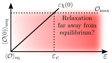
Figure 1: (Color online) While for weak external forces, the initial expectation value $\langle{\cal O}(0)\rangle_{\text{neq}}$ follows the linear prediction in Eq. (5), this prediction has to break down at the latest for a perturbation of strength $\varepsilon_{\text{c}}$, cf. Eq. (8). Here, we study the relaxation dynamics of initial states in the entire regime close to as well as far away from equilibrium.

III Nonequilibrium dynamics and correlation functions

High temperatures and arbitrary perturbations

Although the states $\rho_{\text{neq}}$ in Eq. (1) do not require a specific type of operator, we here restrict ourselves to so-called binary operators ${\cal O}_{l}=c_{1}({\cal P}+c_{2})$, where all eigenvalues of ${\cal P}$ are either $0$ or $1$, and $c_{1}$ and $c_{2}$ are some real constants. Then, ${\cal P}^{2}={\cal P}$ and ${\cal P}$ describes a projection. Binary operators are, e.g., local fermionic occupation numbers fabricius1998 ; steinigeweg2017_1 ; steinigeweg2017_2 ; karrasch2017 and local energy densities karrasch2017 ; karrasch2014 in the isotropic Heisenberg spin-$1/2$ chain. (These two examples will be considered in our numerical simulations below.)

Moreover, let us focus on the regime of high temperatures and strong external forces, i.e., we want to consider the regime $\beta\to 0$ but $\beta\varepsilon>0$. In this regime, we can write to good approximation

$$\rho_{\text{neq}}\approx\frac{e^{\beta\varepsilon c_{1}({\cal P}+c_{2})}}{\text{Tr}[e^{\beta\varepsilon c_{1}({\cal P}+c_{2})}]}=\frac{e^{\beta\varepsilon c_{1}{\cal P}}}{\text{Tr}[e^{\beta\varepsilon c_{1}{\cal P}}]}\ .$$ (9)

From now on, to simplify notation, we absorb $c_{1}$ in the definition of $\varepsilon$. A Taylor expansion of this exponential, combined with the projection property ${\cal P}^{i}={\cal P}$, then yields

$$\rho_{\text{neq}}\ \propto 1+\beta\varepsilon{\cal P}+\tfrac{1}{2}\beta^{2}\varepsilon^{2}{\cal P}^{2}+\tfrac{1}{6}\beta^{3}\varepsilon^{3}{\cal P}^{3}+\dots$$

$$=1+\beta\varepsilon{\cal P}+\tfrac{1}{2}\beta^{2}\varepsilon^{2}{\cal P}+\tfrac{1}{6}\beta^{3}\varepsilon^{3}{\cal P}+\dots$$

$$=1+(e^{\beta\varepsilon}-1)\,{\cal P}\ .$$ (10)

Next, let us focus the situation where one measures the relaxation of exactly the same observable which is used to prepare the initial state, i.e., we have ${\cal O}_{l^{\prime}}={\cal O}_{l}=c_{1}({\cal P}+c_{2})$. Then, it follows from Eq. (10) that the time-dependent expectation value $\langle{\cal O}_{l^{\prime}}(t)\rangle_{\text{neq}}=c_{1}(\langle{\cal P}(t)\rangle_{\text{neq}}+c_{2})$ is given by the relation

$$\langle{\cal P}(t)\rangle_{\text{neq}}=\frac{\langle{\cal P}\rangle_{\text{eq}}+(e^{\beta\varepsilon}-1)\cdot\langle{\cal P}{\cal P}(t)\rangle_{\text{eq}}}{1+(e^{\beta\varepsilon}-1)\cdot\langle{\cal P}\rangle_{\text{eq}}}\ .$$ (11)

Thus, at high temperatures, the nonequilibrium dynamics of binary operators is generated by the equilibrium correlation function $\langle{\cal P}{\cal P}(t)\rangle_{\text{eq}}$ for all $\varepsilon$, i.e., even beyond the regime of small perturbations. This prediction is a central result of our paper.

In particular, for small $\varepsilon$, Eq. (11) can be linearized (Taylor expansion up to linear order around $\varepsilon=0$) and becomes $\langle{\cal P}(t)\rangle_{\text{neq}}=\langle{\cal P}\rangle_{\text{eq}}+\varepsilon\,\chi_{{\cal P},{\cal P}}(t)$ with

$$\chi_{{\cal P},{\cal P}}(t)\approx\beta\Big{(}\langle{\cal P}{\cal P}(t)\rangle_{\text{eq}}-\langle{\cal P}\rangle_{\text{eq}}^{2}\Big{)}\ ,$$ (12)

as expected from LRT. It is worth pointing out that such a dynamical independence of $\varepsilon$ can hardly be expected at low temperatures. There, the time dependence of $\chi_{{\cal P},{\cal P}}(t)$ is not just given by $\langle{\cal P}{\cal P}(t)\rangle_{\text{eq}}$, cf. Eq. (6).

Arbitrary temperatures and strong perturbations

In addition to the above considerations for $\beta\to 0$, it is also instructive to study the limit of infinitely strong perturbations $\varepsilon\to\infty$ at arbitrary temperatures $\beta\geq 0$. In the following, we will again consider binary operators which fulfill ${\cal P}^{2}={\cal P}$. As discussed in the context of Eq. (7), $\rho_{\text{neq}}$ in Eq. (1) acts as projector in the limit $\varepsilon\to\infty$. Hence, we find

$$\lim_{\varepsilon\to\infty}\rho_{\text{neq}}\propto{\cal P}\,e^{-\beta{\cal H}}\,{\cal P}$$ (13)

and

$$\lim_{\varepsilon\to\infty}\langle{\cal P}(t)\rangle_{\text{neq}}=\tilde{C}(t)=\frac{\langle{\cal P}{\cal P}(t){\cal P}\rangle_{\text{eq}}}{\langle{\cal P}\rangle_{\text{eq}}}\ ,$$ (14)

which is valid for any temperature $\beta\geq 0$. In some cases, $\tilde{C}(t)$ can be connected to the usual correlation function $\langle{\cal P}{\cal P}(t)\rangle_{\text{eq}}$ in Eq. (11). Specifically, one can require some sort of “particle-hole symmetry”, i.e., invariance of $\tilde{C}(t)$ under

$${\cal P}(t)\to 1-{\cal P}(t)\,.$$ (15)

(In fact, this requirement is fulfilled by the local fermionic occupation numbers in the XXZ spin-$1/2$ chain discussed later.) Exploiting this property, one can write

$$\tilde{C}(t)=\frac{\langle[1-{\cal P}][1-{\cal P}(t)][1-{\cal P}]\rangle_{\text{eq}}}{\langle{\cal P}\rangle_{\text{eq}}}\ .$$ (16)

Multiplying out the brackets on the r.h.s. of this relation, using $\langle{\cal P}\rangle_{\text{eq}}=1/2$, and rearranging a bit yields

$$2\langle{\cal P}\,{\cal P}(t)\,{\cal P}\rangle_{\text{eq}}=\langle{\cal P}\,{\cal P}(t)\rangle_{\text{eq}}+\langle{\cal P}(t)\,{\cal P}\rangle_{\text{eq}}\ ,$$ (17)

and, since $\langle{\cal P}(t)\,{\cal P}\rangle_{\text{eq}}=\langle{\cal P}\,{\cal P}(t)\rangle_{\text{eq}}^{*}$,

$$\langle{\cal P}\,{\cal P}(t)\,{\cal P}\rangle_{\text{eq}}=\text{Re}\,\langle{\cal P}\,{\cal P}(t)\rangle_{\text{eq}}\ .$$ (18)

Thus, as a consequence of this identity, we can rewrite the correlation function $\tilde{C}(t)$ as

$$\tilde{C}(t)=\text{Re}\,\frac{\langle{\cal P}\,{\cal P}(t)\rangle_{\text{eq}}}{\langle{\cal P}\rangle_{\text{eq}}}\ .$$ (19)

Comparing Eqs. (14) and (19), the nonequilibrium expectation value $\langle{\cal P}(t)\rangle_{\text{neq}}$ in the limit $\varepsilon\to\infty$ eventually recovers the real part of the equilibrium correlation function $\langle{\cal P}\,{\cal P}(t)\rangle_{\text{eq}}$ at any temperature. This is another main result.

IV Dynamical typicality and pure-state propagation

Time-dependent expectation values of the form $\langle{\cal O}_{l^{\prime}}(t)\rangle_{\text{neq}}=\text{Tr}[\rho_{\text{neq}}(t){\cal O}_{l^{\prime}}]$ can be calculated exactly, if the eigenstates and eigenvalues of the Hamiltonians ${\cal H}-\varepsilon{\cal O}_{l}$ and ${\cal H}$ are obtained from the exact diagonalization (ED) of finite systems. But, in addition to the main limitation set by the exponential growth of many-body Hilbert spaces, this procedure is also costly since it requires to perform the exact diagonalization of two operators. Therefore, we here proceed differently and rely on the concept of dynamical typicality (QT) gemmer2003 ; goldstein2006 ; popescu2006 ; reimann2007 ; bartsch2009 ; bartsch2011 ; sugiura2012 ; sugiura2013 ; elsayed2013 ; hams2000 ; iitaka2003 ; iitaka2004 ; white2009 ; monnai2014 . This concept states that a single pure state can have the same properties as the ensemble density matrix. Precisely, the main idea is to replace the trace $\text{Tr}[\rho_{\text{neq}}\mathcal{O}_{l^{\prime}}(t)]$ by the scalar product $\bra{\phi}\rho_{\text{neq}}\mathcal{O}_{l^{\prime}}(t)\ket{\phi}$, where the pure state $\ket{\phi}$ is drawn at random according to the unitary invariant Haar measure bartsch2009 ; bartsch2011 . By the use of this replacement, the expectation value $\langle{\cal O}_{l^{\prime}}(t)\rangle_{\text{neq}}$ can be written as

$$\langle{\cal O}_{l^{\prime}}(t)\rangle_{\text{neq}}=\bra{\psi_{\text{neq}}(t)}{\cal O}_{l^{\prime}}\ket{\psi_{\text{neq}}(t)}+f(\ket{\phi})$$ (20)

with the nonequilibrium pure state $\ket{\psi_{\text{neq}}(t)}=e^{-i\mathcal{H}t}\ket{\psi_{\text{neq}}(0)}$ and

$$\ket{\psi_{\text{neq}}(0)}=\frac{\sqrt{\rho_{\text{neq}}}\ket{\phi}}{\sqrt{\langle\phi|\rho_{\text{neq}}|\phi\rangle}}\ .$$ (21)

Note that the statistical error in Eq. (20) scales as $f(\ket{\phi})\propto 1/d_{\text{eff}}^{1/2}$, where $d_{\text{eff}}={\cal Z}_{\text{neq}}/e^{-\beta E_{\text{neq}}}$ is the effective dimension of the Hilbert space and $E_{\text{neq}}$ denotes the energy of the ground state. Thus, as the size of a many-body quantum system is increased, $f(\ket{\phi})$ vanishes exponentially fast and can be neglected for medium system sizes already steinigeweg2014 ; steinigeweg2015 (cf. Appendix B and C). For a recent discussion of dynamical typicality and similar classes of pure states, see Ref. reimann2018 . Note further, that the concept of typicality has also been recently used to study linear and nonlinear responses in a different but related setup Endo2018 .

Relying on the QT relation in Eq. (20) we do not need to deal with density matrices and can consider pure states instead. Moreover, given the class of pure states (21) in combination with Eqs. (11) and (19), only a single state is required, compared to earlier calculations of correlation functions based on two (auxiliary) pure states steinigeweg2014 ; steinigeweg2015 . While a forward propagation w.r.t. ${\cal H}-\varepsilon{\cal O}_{l}$ in imaginary time $\beta$ allows us to prepare $\ket{\psi_{\text{neq}}(0)}$, another forward propagation w.r.t. ${\cal H}$ in real time $t$ allows us to calculate $\ket{\psi_{\text{neq}}(t)}$. The main advantage of the pure-state approach comes from the fact that these propagations can be done by iteratively solving the Schrödinger equation (in real and imaginary time), e.g., by a fourth-order Runge-Kutta scheme with a small time step $\delta t$ elsayed2013 ; steinigeweg2014 ; steinigeweg2015 ; herbrych2016 . This scheme does not require exact diagonalization and, due to the fact that few-body operators are relatively sparse, also the matrix-vector multiplications can be implemented in a very memory-efficient way. Hence, in comparison to exact diagonalization, we can treat systems with much larger Hilbert spaces. Note that also more sophisticated schemes can be applied such as Trotter decompositions or Chebyshev polynomials steinigeweg2017_1 ; steinigeweg2017_2 ; weisse2006 . However, for the purposes of our paper, i.e., the numerical illustration of our analytical results, Runge-Kutta will be sufficient.

V Numerical Illustration

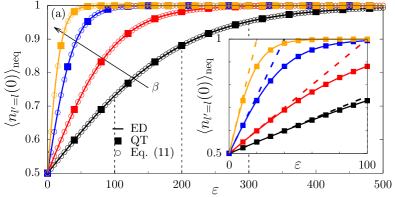
Figure 2: (Color online) (a) Static expectation value $\langle n_{l^{\prime}=l}(0)\rangle_{\text{neq}}$ versus perturbation $\varepsilon$ for high temperatures $\beta=0.01$, $0.02$, $0.05$, and $0.1$ (arrow). Exact diagonalization (ED) is compared to quantum typicality (QT). The analytical prediction in Eq. (11) is depicted for comparison. The vertical dashed lines indicate those values of $\varepsilon$ which will be used to study the nonequilibrium dynamics in the following. (b) Same data as in (a) but shown for $\varepsilon\leq 100$ only. The LRT prediction in Eq. (5) is now indicated (dashed line). Parameters: $\Delta=1$ and $\delta t=0.01$ as well as $L=8$ (ED) and $L=24$ (QT).

V.1 Model

Next, we turn to our numerical simulations and study, as an example, nonequilibrium dynamics in the XXZ spin-1/2 chain. The Hamiltonian of this chain reads (with periodic boundary conditions) $\mathcal{H}=\sum_{l=1}^{L}h_{l}$,

$$h_{l}=J\left(S_{l}^{x}S_{l+1}^{x}+S_{l}^{y}S_{l+1}^{y}+\Delta S_{l}^{z}S_{l+1}^{z}\right)\ ,$$ (22)

where $S_{l}^{x,y,z}$ are spin-$1/2$ operators at site $l$, $L$ is the number of sites, $J=1$ is the antiferromagnetic exchange coupling constant, and $\Delta$ is the anisotropy. By the use of the Jordan-Wigner transformation, this Hamiltonian can be also mapped onto a one-dimensional model of spinless fermions with interactions between nearest neighbors. In this picture, the operator $n_{l}=S_{l}^{z}+1/2$ becomes a local fermionic occupation number. Because such an operator has only the two eigenvalues $0$ and $1$, it naturally fulfills the projection property $n_{l}^{2}=n_{l}$. Consequently, we prepare the initial state $\rho_{\text{neq}}$ by using the choice ${\cal O}_{l}=n_{l}$ and subsequently measure the observable ${\cal O}_{l^{\prime}}=n_{l^{\prime}}$. In fact, we here restrict ourselves for simplicity to the single case $l=l^{\prime}$. Note that our numerical simulations are performed for all subsectors of fixed magnetization $S^{z}=\sum_{l}S_{l}^{z}$ (or, in the fermionic language, all subsectors of fixed particle number $N=\sum_{l}n_{l}$).

V.2 Results

Static expectation values

We now discuss our numerical results. First, we study the influence of the perturbation $\varepsilon$ on static expectation values, i.e., we investigate the validity range of the LRT prediction in Eq. (5) at $t=0$. In Fig. 2 (a) we show $\langle n_{l^{\prime}=l}(0)\rangle_{\text{neq}}$ for a wide range $\varepsilon\leq 500$, high temperatures $\beta=0.01$, $0.02$, $0.05$, and $0.1$, as well as anisotropy $\Delta=1$. At $\varepsilon=0$, we have $\langle n_{l^{\prime}=l}(0)\rangle_{\text{neq}}=\langle n_{l^{\prime}=l}\rangle_{\text{eq}}=1/2$. As $\varepsilon$ increases, we observe a linear growth of $\langle n_{l^{\prime}=l}(0)\rangle_{\text{neq}}$ with $\varepsilon$. As depicted in Fig. 2 (b), this linear growth is very well described by the LRT prediction in Eq. (5) and $\chi_{l,l^{\prime}=l}=\beta/4$. For large $\varepsilon$, $\langle n_{l^{\prime}=l}(0)\rangle_{\text{neq}}$ eventually saturates at the constant value $\langle n_{l^{\prime}=l}(0)\rangle_{\text{neq}}=1$. This saturation is expected due to Eq. (7) and the maximum eigenvalue $n_{l,\text{max}}=1$. In Figs. 2 (a) and (b), the QT relation in Eq. (20) is additionally confirmed by a direct comparison with data from exact diagonalization. For all $\beta$ considered here, the statistical error $f(\ket{\phi})$ turns out to be negligibly small. Overall, the numerical results in Figs. 2 (a) and (b) confirm our analytical predictions. In particular, static LRT breaks down for sufficiently large $\varepsilon$. As an additional orientation, the vertical dashed lines in Fig. 2 (a) indicate those values of $\varepsilon$ which will be used to study the nonequilibrium dynamics in the following. Note that these values are chosen in such a way that we cover the whole range from states inside the linear regime, as well as initial states which are almost maximally perturbed.

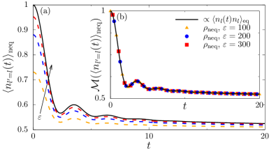
Figure 3: (Color online) (a) Time evolution of the expectation value $\langle n_{l^{\prime}=l}(t)\rangle_{\text{neq}}$ for perturbations $\varepsilon=100$, $200$, and $300$ (arrow) at a high temperature $\beta=0.01$. As a comparison, the (normalized) equilibrium correlation function $\langle n_{l}(t)n_{l}\rangle_{\text{eq}}$ is shown. (b) Data collapse of (a) using a simple linear map. Parameters: $L=28$ and $\delta t=0.01$ as well as $\Delta=1$.

Dynamical expectation values

Next, we turn to dynamical expectation values, with the focus on a high temperature $\beta=0.01$. In Fig. 3 (a) we depict $\langle n_{l^{\prime}=l}(t)\rangle_{\text{neq}}$ for perturbations $\varepsilon=100$, $200$, and $300$, as resulting from the QT relation (20). Further, as a comparison, we depict the (normalized) equilibrium correlation function $\langle n_{l}(t)n_{l}\rangle_{\text{eq}}$, which can be calculated by means of a pure-state approach as well steinigeweg2014 ; steinigeweg2015 . While we observe that all curves shown differ from each other, this observation is not surprising because, as illustrated in Fig. 2, the initial values $\langle n_{l^{\prime}=l}(0)\rangle_{\text{neq}}$ depend on $\varepsilon$. In view of this fact, we try a data collapse using the simple map (see Appendix A)

$${\cal M}(\langle n_{l^{\prime}=l}(t)\rangle_{\text{neq}})=a\ \langle n_{l^{\prime}=l}(t)\rangle_{\text{neq}}+b\ ,$$ (23)

where the strictly time-independent coefficients $a$ and $b$ can be chosen as

$$a=\frac{n_{l,max}-\langle n_{l^{\prime}=l}\rangle_{\text{eq}}}{\langle n_{l^{\prime}=l}\rangle_{\text{neq}}-\langle n_{l^{\prime}=l}\rangle_{\text{eq}}}\,,\quad b=(1-a)\langle n_{l^{\prime}=l}\rangle_{\text{eq}}\ .$$ (24)

Note that in the case of a traceless operator, $\langle\mathcal{O}\rangle_{\text{eq}}=0$, this map essentially reduces to a normalization of the data to the initial value,

$${\cal M}(\langle\mathcal{O}(t)\rangle_{\text{neq}})\propto\frac{\langle\mathcal{O}(t)\rangle_{\text{neq}}}{\langle\mathcal{O}(0)\rangle_{\text{neq}}}\ .$$ (25)

Due to our discussion in the context of Eqs. (5) and (11), such a linear map is reasonable for small and large $\varepsilon$. And indeed, as shown in Fig. 3 (b), the rescaled curves lie on top of each other for all values of $\varepsilon$. This finding is a main result of our paper, as it clearly confirms our analytical prediction in Eq. (11) that the dynamical behavior at high temperatures, even outside the linear response regime, is generated by a single equilibrium correlation function, at least for binary operators. Moreover, it is worth noting that the data is presented for system size $L=28$, substantially beyond what is possible in conventional ED fabricius1998 .

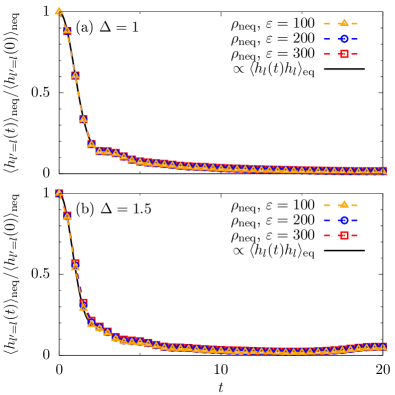
Figure 4: (Color online) Time evolution of the expectation value $\langle h_{l^{\prime}=l}(t)\rangle_{\text{neq}}$ for perturbations $\varepsilon=100$, $200$, and $300$ (arrow) at a high temperature $\beta=0.01$ for (a) $\Delta=1$ and (b) $\Delta=1.5$. As a comparison, the (normalized) equilibrium correlation function $\langle h_{l}(t)h_{l}\rangle_{\text{eq}}$ is shown. Other parameters: $L=28$ ($\Delta=1$), $L=24$ ($\Delta=1.5$), and $\delta t=0.01$.

The local fermionic occupation numbers $n_{l}$ considered so far appear in various physical models, not just in the Heisenberg model or in one dimension. To demonstrate, however, that our results are not restricted to such $n_{l}$, we extend our analysis to other operators and consider the local energy density $h_{l}$ in Eq. (22). This local energy density is a spin dimer. For anisotropy $\Delta=1$, this dimer features a triplet state ($\ket{\uparrow\uparrow}$, $\ket{\downarrow\downarrow}$, $\ket{\uparrow\downarrow}+\ket{\downarrow\uparrow}$) with energy $E_{\text{t}}=1/4$ and a singlet ground state ($\ket{\uparrow\downarrow}-\ket{\downarrow\uparrow}$) with energy $E_{\text{s}}=-3/4$. Hence, Eq. (11) holds for the projector ${\cal P}=h_{l}-E_{\text{s}}$, and dynamical independence of the perturbation is obviously expected for the choice ${\cal O}_{l}=h_{l}$ as well. Indeed, as shown in Fig.  4 (a), the rescaled expectation values $\langle h_{l^{\prime}=l}(t)\rangle_{\text{neq}}$ for different perturbations $\varepsilon$ all lie on top of each other. Therefore, our results are clearly valid for a larger class of binary operators.

Nonbinary operators

The natural question arises if and to what extend our results also apply to nonbinary operators. To work towards an answer of this question let us also consider a larger anisotropy $\Delta=1.5$. In this case, the local energy density $h_{l}$ becomes a nonbinary operator (since the degeneracy of the triplet state is partially lifted). As a consequence, ${\cal P}=h_{l}-E_{\text{s}}$ does not fulfill the projection property, ${\cal P}^{2}\neq{\cal P}$, and our derivation from Eq. (10) will certainly break down. Thus, we cannot expect a priori that the relaxation dynamics is still independent of the perturbation $\varepsilon$. However, as depicted in Fig. 4 (b), the numerical results reveal that even for this example of a nonbinary operator, the dynamics are still very well generated by a single correlation function. Although this finding cannot be explained within the framework discussed in the paper at hand, it suggests that there might exist a more general theory for arbitrary operators.

Lower temperatures

In the context of Eqs. (10) and (11) we proved that at high temperatures the nonequilibrium dynamics of binary operators is already characterized by a single equilibrium correlation function. Moreover, we numerically confirmed this prediction in Figs. 3 and 4 (a) by demonstrating that the relaxation curves for different perturbation strengths $\varepsilon$ lie on top of each other after the simple linear map. Clearly, such an independence of $\varepsilon$ can hardly be expected at low temperatures. However, it may occur over a wider range of high temperatures $\beta>0.01$. Thus, we redo the calculation for $\langle n_{l^{\prime}=l}(t)\rangle_{\text{neq}}$ in Figs. 3 (a) and (b) for the lower temperature $\beta=1$ and depict the corresponding results in Figs. 5 (a) and (b). For comparison, we also show the (normalized) correlation function $\langle n_{l}(t)n_{l}\rangle_{\text{eq}}$ at $\beta=1$. While the data collapse is certainly not as good as before, it is still convincing.

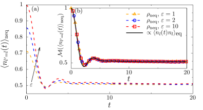
Figure 5: (Color online) (a) Time evolution of the expectation value $\langle n_{l^{\prime}=l}(t)\rangle_{\text{neq}}$ for perturbations $\varepsilon=1$, $2$, and $10$ (arrow) at a lower temperature $\beta=1$. (b) Rescaling of (a) using a simple linear map. As a comparison, the (normalized) equilibrium correlation function $\langle n_{l}(t)n_{l}\rangle_{\text{eq}}$ is shown. Parameters: $L=24$, $\delta t=0.01$, and $\Delta=1$.

VI Conclusion

To summarize, we have studied the nonequilibrium dynamics for a class of initial states resulting from a certain type of quench. Specifically, we considered thermal states of the system in the presence of an additional external force which, however, become nonequilibrium states when this force is eventually removed. Moreover, by tuning the strength of the external force, these states can be prepared close to as well as far away from equilibrium, i.e., inside as well as outside the linear response regime, at arbitrary temperature.

In particular, we discussed the case of so-called binary operators and specific examples for such observables. For these operators we proved that the nonequilibrium dynamics at high temperatures is characterized by a single correlation function evaluated exactly at equilibrium, even in the case of arbitrarily strong perturbations. This analytical result can also help to understand earlier numerical experiments where nonequilibrium dynamics has been related to linear response theory karrasch2017 ; Karrasch2013 .

In order to verify our results, we employed an efficient numerical approach based on the concept of dynamical typicality and studied the nonequilibrium dynamics in the spin-$1/2$ XXZ chain. In addition to confirming our analytical predictions, these simulations also provided evidence that our results might be (at least qualitatively) applicable in a much wider context, i.e., lower temperatures as well as more general types of operators. Albeit our numerical examples are certainly very different, it is in this context also worth mentioning two very recent experiments where universal dynamics in a far-from-equilibrium situation has been observed Prufer2018 ; Erne2018 .

Promising future directions of research include the analysis of non-binary operators and low temperatures (in more detail), as well as the application of the pure-state approach to specific questions in many-body quantum systems. In this context, the study of nonequilibrium dynamics, transport properties, and thermalization in disordered systems is one important example Richter2018_2 . Moreover, a very recent work richter2018 shows that our results also hold true for a wider class of generic observables and models, as long as the off-diagonal eigenstate thermalization hypothesis applies.

Acknowledgments

This work has been funded by the Deutsche Forschungsgemeinschaft (DFG) - STE 2243/3-1. We sincerely thank J. Gemmer, P. Reimann, J. Herbrych, and the members of the DFG Research Unit FOR 2692 for fruitful discussions.

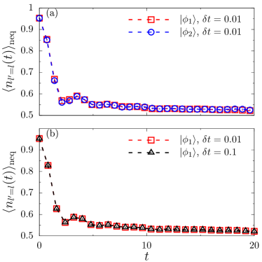
Figure 6: (Color online) Analysis of errors. Time evolution of the expectation value $\langle n_{l^{\prime}=l}(t)\rangle_{\text{neq}}$ for perturbation $\varepsilon=300$, temperature $\beta=0.01$, anisotropy $\Delta=1$, and system size $L=16$, as resulting for: (a) two different reference states $\ket{\phi_{1}}$ and $\ket{\phi_{2}}$, (b) two different Runge-Kutta time steps $\delta t=0.01$ and $0.1$.

Appendix A Linear Map

The time-independent coefficients of the linear map in Eq. (23) follow from two conditions. The first condition is about the initial value, i.e.,

$$a\ \langle n_{l^{\prime}=l}(t=0)\rangle_{\text{neq}}+b=c_{0}\ .$$ (26)

The second condition is about the long-time value, i.e.,

$$a\ \langle n_{l^{\prime}=l}(t\to\infty)\rangle_{\text{neq}}+b=c_{\infty}\ .$$ (27)

We choose $c_{0}=n_{l,max}$ and $c_{\infty}=\langle n_{l^{\prime}=l}\rangle_{\text{eq}}$ and get the parameters

$$a=\frac{n_{l,max}-\langle n_{l^{\prime}=l}\rangle_{\text{eq}}}{\langle n_{l^{\prime}=l}\rangle_{\text{neq}}-\langle n_{l^{\prime}=l}\rangle_{\text{eq}}}$$ (28)

and $b=(1-a)\langle n_{l^{\prime}=l}\rangle_{\text{eq}}$. Other choices are also possible, of course.

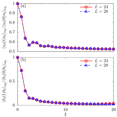
Figure 7: (Color online) Time evolution of the (normalized) equilibrium correlation functions (a) $\langle n_{l}(t)n_{l}\rangle_{\text{eq}}$ and (b) $\langle h_{l}(t)h_{l}\rangle_{\text{eq}}$ for anisotropy $\Delta=1$ and two different system sizes $L=24$ and $L=28$.

Appendix B Error Analysis

Eventually, let us further comment on the accuracy of our pure-state approach, i.e., of the typicality relation in Eq. (20) of the main text. While the comparison with exact diagonalization in Fig. 2 has illustrated this accuracy already for static expectation values, there is another convenient way to demonstrate the smallness of statistical errors. This way is the comparison of results for two or even more instances of the reference state $\ket{\phi}$ in Eq. (21). Note that a single instance of this pure state is $\ket{\phi}=\sum_{k}c_{k}\ket{\varphi_{k}}$, where the real and imaginary part of the complex coefficients $c_{k}$ are drawn at random according to a Gaussian distribution with zero mean and $\ket{\varphi_{k}}$ is the Ising basis.

In Fig. 6 (a) we exemplarily compare the dynamical expectation values $\langle n_{l^{\prime}=l}(t)\rangle_{\text{neq}}$ for two different random realizations $\ket{\phi_{1}}$ and $\ket{\phi_{2}}$. For both realizations, we use the same perturbation $\varepsilon=300$, temperature $\beta=0.01$, and system size $L=16$. Since the two curves coincide almost perfectly, we can conclude that statistical errors are indeed very small, even for chains with only $L=16$ sites. Because these errors decrease exponentially fast as the number of sites increases, our calculations for larger system sizes $L=28$ in the main text can be considered as practically exact.

Eventually, we compare in Fig. 6 (b) the time evolution of the expectation value $\langle n_{l^{\prime}=l}(t)\rangle_{\text{neq}}$ for the same set of parameters but two different Runge-Kutta time steps $\delta t=0.01$ and $0.1$. As the curves do not differ for these two choices, the time step $\delta t=0.01$ chosen throughout our paper is certainly small enough to ensure negligibly small numerical errors.

Appendix C Finite-Size Effects

While it is evident from Fig. 2 that finite-size effects are negligibly small for static expectation values, let us also comment briefly on finite-size effects for dynamical expectation values. To this end, we compare in Fig. 7 numerical data for two different system sizes $L=24$ and $L=28$. Apparently, for $\langle n_{l}(t)n_{l}\rangle_{\text{eq}}$ in Fig. 7 (a), both curves coincide with each other, at least for all times $t\leq 20$ depicted. (Data from exact diagonalization can be found for small $L=16\ll 28$ in fabricius1998 ). For $\langle h_{l}(t)h_{l}\rangle_{\text{eq}}$ in Fig. 7 (b), one can see minor deviations at times $t\sim 20$.

However, we should stress that such finite-size effects do not affect the conclusions in the main text. In fact, all relations discussed do not require the convergence to the thermodynamic limit.

References

- (1) D. C. Johnston, R. K. Kremer, M. Troyer, X. Wang, A. Klümper, S. L. Bud’ko, A. F. Panchula, and P. C. Canfield, Phys. Rev. B 61, 9558 (2000).
- (2) U. Schollwöck, Rev. Mod. Phys. 77, 259 (2005); Ann. Phys. 326, 96 (2011).
- (3) P. Prelovšek and J. Bonča, Ground State and Finite Temperature Lanczos Methods, Solid-State Sciences 176 (Springer, Berlin, 2013).
- (4) A. Eckardt, C. Weiss, and M. Holthaus, Phys. Rev. Lett. 95, 260404 (2005).
- (5) A. Lazarides, A. Das, and R. Moessner, Phys. Rev. Lett. 112, 150401 (2014).
- (6) M. Campisi, P. Hänggi, and P. Talkner, Rev. Mod. Phys. 83, 771 (2011).
- (7) C. Mejía-Monasterio, T. Prosen, and G. Casati, EPL (Europhys. Lett.) 72, 520 (2005).
- (8) M. Michel, O. Hess, H. Wichterich, and J. Gemmer, Phys. Rev. B 77, 104303 (2008).
- (9) M. Žnidarič, Phys. Rev. Lett. 106, 220601 (2011).
- (10) T. Langen, R. Geiger, and J. Schmiedmayer, Annu. Rev. Condens. Matter Phys. 6, 201 (2015).
- (11) R. Nandkishore and D. A. Huse, Annu. Rev. Condens. Matter Phys. 6, 15 (2015).
- (12) J. Eisert, M. Friesdorf, and C. Gogolin, Nature Phys. 11, 124 (2015).
- (13) L. D’Alessio, Y. Kafri, A. Polkovnikov, and M. Rigol, Adv. Phys. 65, 239 (2016).
- (14) J. M. Deutsch, Phys. Rev. A 43, 2046 (1991).
- (15) M. Srednicki, Phys. Rev. E 50, 888 (1994).
- (16) M. Rigol, V. Dunjko, and M. Olshanii, Nature 452, 854 (2008).
- (17) J. Gemmer and G. Mahler, Eur. Phys. J. B 31, 249 (2003).
- (18) S. Goldstein, J. L. Lebowitz, R. Tumulka, and N. Zanghì, Phys. Rev. Lett. 96, 050403 (2006).
- (19) S. Popescu, A. J. Short, and A. Winter, Nature Phys. 2, 754 (2006).
- (20) P. Reimann, Phys. Rev. Lett. 99, 160404 (2007).
- (21) C. Bartsch and J. Gemmer, Phys. Rev. Lett. 102, 110403 (2009).
- (22) C. Bartsch and J. Gemmer, EPL (Europhys. Lett.) 96, 60008 (2011).
- (23) S. Sugiura and A. Shimizu, Phys. Rev. Lett. 108, 240401 (2012).
- (24) S. Sugiura and A. Shimizu, Phys. Rev. Lett. 111, 010401 (2013).
- (25) T. A. Elsayed and B. V. Fine, Phys. Rev. Lett. 110, 070404 (2013).
- (26) A. Hams and H. De Raedt, Phys. Rev. E 62, 4365 (2000).
- (27) T. Iitaka and T. Ebisuzaki, Phys. Rev. Lett. 90, 047203 (2003).
- (28) T. Iitaka and T. Ebisuzaki, Phys. Rev. E 69, 057701 (2004).
- (29) S. R. White, Phys. Rev. Lett. 102, 190601 (2009).
- (30) T. Monnai and A. Sugita, J. Phys. Soc. Jpn. 83, 094001 (2014).
- (31) P. Reimann, Nature Commun. 7, 10821 (2016).
- (32) L. P. García-Pintos, N. Linden, A. S. L. Malabarba, A. J. Short, and A. Winter, Phys. Rev. X 7, 031027 (2017).
- (33) R. Kubo, M. Toda and, N. Hashitsume, Statistical Physics II: Nonequilibrium Statistical Mechanics, Solid-State Sciences 31 (Springer, Berlin, 1991).
- (34) C. Karrasch, J. H. Bardarson, and J. E. Moore, Phys. Rev. Lett. 108, 227206 (2012).
- (35) T. Prosen, Phys. Rev. Lett. 106, 217206 (2011).
- (36) T. Prosen and E. Ilievski, Phys. Rev. Lett. 111, 057203 (2013).
- (37) R. Steinigeweg, J. Gemmer, and W. Brenig, Phys. Rev. Lett. 112, 120601 (2014).
- (38) R. Steinigeweg, J. Gemmer, and W. Brenig, Phys. Rev. B 91, 104404 (2015).
- (39) K. Fabricius and B. M. McCoy, Phys. Rev. B 57, 8340 (1998).
- (40) R. Steinigeweg, F. Jin, D. Schmidtke, H. de Raedt, K. Michielsen, and J. Gemmer, Phys. Rev. B 95, 035155 (2017).
- (41) R. Steinigeweg, F. Jin, H. De Raedt, K. Michielsen, and J. Gemmer, Phys. Rev. E 96, 020105(R) (2017).
- (42) C. Karrasch, T. Prosen, and F. Heidrich-Meisner, Phys. Rev. B 95, 060406(R) (2017).
- (43) C. Karrasch, J. E. Moore, and F. Heidrich-Meisner, Phys. Rev. B 89, 075139 (2014).
- (44) Not for every observable there is a force luttinger1964 ; zwanzig1965 ; gemmer2006 .
- (45) J. M. Luttinger, Phys. Rev. 135, A1505 (1964).
- (46) R. Zwanzig, Annu. Rev. Phys. Chem. 16, 67 (1965).
- (47) J. Gemmer, R. Steinigeweg, and M. Michel, Phys. Rev. B 73, 104302 (2006).
- (48) F. H. L. Essler, S. Kehrein, S. R. Manmana, and N. J. Robinson, Phys. Rev. B 89, 165104 (2014).
- (49) C. Bartsch and J. Gemmer, EPL (Europhys. Lett.) 118, 10006 (2017).
- (50) R. L. Peterson, Rev. Mod. Phys. 39, 69 (1967).
- (51) P. Reimann, Phys. Rev. E 97, 062129 (2018).
- (52) H. Endo, C. Hotta, and A. Shimizu, Phys. Rev. Lett. 121, 220601 (2018).
- (53) J. Herbrych and X. Zotos, Phys. Rev. B 93, 134412 (2016).
- (54) A. Weiße, G. Wellein, A. Alvermann, and H. Fehske, Rev. Mod. Phys. 78, 275 (2006).
- (55) C. Karrasch, R. Ilan, and J. E. Moore, Phys. Rev. B 88, 195129 (2013).
- (56) M. Prüfer, P. Kunkel, H. Strobel, S. Lannig, D. Linnemann, C-M. Schmied, J. Berges, T. Gasenzer, and M. K. Oberthaler, Nature 563, 217 (2018).
- (57) S. Erne, R. Bücker, T. Gasenzer, J. Berges, and J. Schmiedmayer, Nature 563, 225 (2018).
- (58) J. Richter, J. Herbrych, and R. Steinigeweg, Phys. Rev. B 98, 134302 (2018).
- (59) J. Richter, J. Gemmer, and R. Steinigeweg, arXiv:1805.11625.