Concave Losses for Robust Dictionary Learning

Abstract

Traditional dictionary learning methods are based on quadratic convex loss function and thus are sensitive to outliers. In this paper, we propose a generic framework for robust dictionary learning based on concave losses. We provide results on composition of concave functions, notably regarding supergradient computations, that are key for developing generic dictionary learning algorithms applicable to smooth and non-smooth losses. In order to improve identification of outliers, we introduce an initialization heuristic based on undercomplete dictionary learning. Experimental results using synthetic and real data demonstrate that our method is able to better detect outliers, is capable of generating better dictionaries, outperforming state-of-the-art methods such as K-SVD and LC-KSVD.

Index Terms—  Robust dictionary learning, outlier detection, concave loss function.

1 Introduction

Dictionary Learning is an important and widely used tool in Signal Processing and Computer Vision. Its versatility is well acknowledged and it can be applied for denoising or for representation learning prior to classification [1, 2]. The method consists in learning a set of overcomplete elements (or atoms) which are useful for describing examples at hand. In this context, each example is represented as a potentially sparse linear span of the atoms. Formally, given a data matrix composed of $n$ elements of dimension $d$, $\mathbf{X}\in\mathbb{R}^{d\times n}$ and each column being an example $\mathbf{x}_{i}$, the dictionary learning problem is given by:

$$\min_{\mathbf{D}\in\mathbb{R}^{d\times k},\mathbf{A}\mathbb{R}^{k\times n}}\frac{1}{2}\sum_{i=1}^{n}\|\mathbf{x}_{i}-\mathbf{D}\mathbf{a}_{i}\|_{2}^{2}+\Omega_{D}(\mathbf{D})+\Omega_{A}(\mathbf{A})$$ (1)

where $\Omega_{D}$ and $\Omega_{A}$ represent some constraints and/or penalties on the dictionary set $\mathbf{D}$ and the matrix coefficient $\mathbf{A}$, each column being a linear combination coefficients $\mathbf{a}_{i}$ so that $\mathbf{x}_{i}\approx\mathbf{D}\mathbf{a}_{i}$. Typical regularizers are sparsity-inducing penalty on $\mathbf{A}$, or unit-norm constraint on each dictionary element although a wide variety of penalties can be useful [3, 4, 5].

As depicted by the mathematical formulation of the problem, the learned dictionary $\mathbf{D}$ depends on training examples $\{\mathbf{x}_{i}\}_{i=1}^{n}$. However, because of the quadratic loss function in the data fitting term, $\mathbf{D}$ is in addition, very sensitive to outlier examples. Our goal here is to address the robustness of the approach to outliers. For this purpose, we consider loss functions that downweight the importance of outliers in $\mathbf{X}$ making the learned dictionary less sensitive to them.

Typical approaches in the literature, that aim at mitigating influence of outliers, use Frobenius norm or component-wise $\ell_{1}$ norm as data-fitting term instead of the squared-Frobenius one [6, 7]. Some works propose loss functions such as the $\ell_{q}$ function, with $q\leq 1$ function or the capped function $g(u)=\min(u,\epsilon)$, for $u>0$ [8, 9]. Due to these non-smooth and non-convex loss function, the resulting dictionary learning problem is more difficult to solve than the original one given in Equation (1). As such, authors have developed algorithms based on a iterative reweighted least-square approaches tailored to the loss function $\ell_{q}$ or $\min(u,\epsilon)$ [8, 9].

Our contribution in this paper is: (i) to introduce a generic framework for robust dictionary learning by considering as loss function the composition of the Frobenius norm and some concave loss functions (our framework encompasses previously proposed methods while enlarging the set of applicable loss functions); (ii) to propose a generic majorization-minimization algorithm applicable to concave, smooth or non-smooth loss functions. Furthermore, because the resulting learning problem is non-convex, its solution is sensitive to initial conditions, hence we propose a novel heuristic for dictionary initialization that helps in detecting outliers more efficiently during the learning process.

2 Concave Robust Dictionary Learning

2.1 Framework and Algorithm

In order to robustify the dictionary learning process against outliers, we need a learning problem that puts less emphasis on examples that are not “correctly” approximated by the learned dictionary. Hence, we propose the following generic learning problem:

$$\min_{\mathbf{D},\mathbf{A}}\frac{1}{2}\sum_{i}F(\|\mathbf{x}_{i}-\mathbf{D}\mathbf{a}_{i}\|_{2}^{2})+\Omega_{D}(\mathbf{D})+\Omega_{A}(\mathbf{A}).$$ (2)

where $F(\bullet)$ is a function over $\mathbb{R}_{>0}$. Note that in the sequel, we will not focus on the penalty and constraints over the dictionary elements and coefficients $\mathbf{A}$. Hence, we consider them as the classical unit-norm constraint over $\mathbf{d}_{j}$ and the $\ell_{1}$ sparsity-inducing penalty over $\{\mathbf{a}_{i}\}$.

Concavity of $F$ is crucial for robustness as it helps in down-weighting influence of large $\|\mathbf{x}_{i}-\mathbf{D}\mathbf{a}_{i}\|_{2}$. For instance, if we set $F(\bullet)=\sqrt{\bullet}$, the above problem is similar to the convex robust dictionary learning proposed by Wang et al. [7]. In order to provide better robustness, our goal is to introduce a generic form of $F$ that leads to a concave loss with respect to $\|\mathbf{x}_{i}-\mathbf{D}\mathbf{a}_{i}\|_{2}$. instead of a linear, yet concave one as in [7].

In this work, we emphasize robustness by considering $F$ as the composition of two concave functions $F(\bullet)=g(\bullet)\circ\sqrt{\bullet}$, with $g$ a non-decreasing concave function over $\mathbb{R}_{>0}$, such as those used for sparsity-inducing penalties. Typically, $g(\bullet)$ can be the $q-$power, $q\leq 1$ function $u^{q}$, the log function $\log(\epsilon+{u})$, the SCAD function [10], or the capped-$\ell_{1}$ function $\min(u,\epsilon)$, or the MCP function [11]. A key property on $F$ is that concavity is preserved by the composition of some specific concave functions as proved by the following lemma which proof is omitted for space reasons.

Lemma 1

Let $g$ be a non-decreasing concave function on $\mathbb{R}_{>0}$ and $h$ be a concave function on a domain $\Omega$ to $\mathbb{R}_{>0}$, then $g\circ h$ is concave. Furthermore, if $g$ is an increasing function then $g\circ h$ is strictly concave.

In our framework, $h$ is the square-root function with $\Omega=\mathbb{R}_{>0}$. In addition, functions $g$, such as those given above, are either a concave or strictly concave functions and are all non-decreasing, hence $F=g\circ h$ is concave. Owing to concavity, for any $u_{0}$ and $u$ in $\mathbb{R}_{>0}$,

$$F(u)\leq F(u_{0})+F^{\prime}(u_{0})(u-u_{0})$$

where $F^{\prime}(u_{0})$ is an element of the superdifferential of $F$ at $u_{0}$. As $F$ is concave, the superdifferential is always non-empty and if $F$ is smooth at $u_{0}$, then $F^{\prime}(u_{0})$ is simply the gradient of $F$ at $u_{0}$. However, since $F$ is a composition of functions, in a non-smooth case, computing superdifferential is difficult unless the inner function is a linear function [12]. Next lemma provides a key result showing that a supergradient of $g\circ\sqrt{\bullet}$ can be simply computed using chain rule because $\sqrt{\bullet}$ is a bijective function on $\mathbb{R}_{>0}$ to $\mathbb{R}_{>0}$ and $g$ is non-decreasing.

Lemma 2

Let $g$ a non-decreasing concave function on $\mathbb{R}_{>0}$ and $h$ a bijective differentiable concave function on a domain $\mathbb{R}_{>0}$ to $\mathbb{R}_{>0}$, then if $g_{1}$ is a supergradient of $g$ at $z$ then $g_{1}\cdot h^{\prime}(s)$ is a supergradient of $g\circ h$ at a point $s$ so that $z=h(s)$.

• As $g_{1}\in\partial g(z)$, we have $\forall y,g(y)\leq g(z)+g_{1}\cdot(y-z)$. Owing to bijectivity of $h$, define $t$ and $s$ so that $y=h(t)$ and $z=h(s)$. In addition, concavity of $h$ gives $h(t)-h(s)\leq h^{\prime}(s)(t-s)$ and because $g$ is non-decreasing, $g_{1}\geq 0$. Combining everything, we have $g_{1}\cdot(y-z)=g_{1}\cdot(h(t)-h(s))\leq g_{1}h^{\prime}(s)(t-s)$. Thus $\forall t,g(h(t))\leq g(h(s))+g_{1}h^{\prime}(s)(t-s)$ which concludes the proof since $g_{1}$ is a supergradient of $g$ at $h(s)$.

Algorithm 1 The proposed Robust DL method

0:  Data matrix $\mathbf{X}\in\mathbb{R}^{d\times n}$, dictionary size $k$, $\lambda$, $\epsilon$, $M$.

1:  if ($k>d$) and (use undercomplete initialization) then

2:     Initialize $\mathbf{D}$ and $s$ with Algorithm 2

3:  else

4:     random initialization of $\mathbf{D}$, $\mathbf{A}$

5:     $s_{j}=1$ for $j=1,\ldots,n$

6:  for $i=1$ to $M$ do

7:     repeat

8:        Update $\mathbf{D}$ by solving Equation 5

9:        for $j=1$ to $n$ do

10:           $\mathbf{a}_{j}\leftarrow\frac{1}{2}||\mathbf{x}_{j}-\mathbf{D}\mathbf{a}||_{2}^{2}+\frac{\lambda}{s_{j}}||\mathbf{a}||_{1}$

11:     until convergence

12:     for $j=1$ to $n$ do

13:        update $s_{j}$ according to Equation 4

13:  $\mathbf{D}$, $s$

Based on the above majorizing linear function property of concave functions and because in our case $F^{\prime}(u_{0})$ can easily be computed, we consider a majorization-minimization approach for solving Problem (2). Our iterative algorithm consists, at iteration $\kappa$, in approximating the concave loss function $F$ at the current solution $\mathbf{D}_{\kappa}$ and $\mathbf{A}_{\kappa}$ and then solve the resulting approximate problem for $\mathbf{D}$ and $\mathbf{A}$. This yields in solving:

$$\min_{\mathbf{D},\mathbf{A}}\frac{1}{2}\sum_{i}s_{i}\|\mathbf{x}_{i}-\mathbf{D}\mathbf{a}_{i}\|_{2}^{2}+\Omega_{D}(\mathbf{D})+\Omega_{A}(\mathbf{A})$$ (3)

where $s_{i}=[g\circ\sqrt{\bullet}\leavevmode\nobreak\ ]^{\prime}$ at $\mathbf{D}_{\kappa}$ and $\mathbf{a}_{\kappa,i}$. Since, we have

$$[g\circ\sqrt{\bullet}\leavevmode\nobreak\ ]^{\prime}(u_{0})=\frac{1}{2\sqrt{u_{0}}}g^{\prime}(\sqrt{u_{0}})$$

weights $s_{i}$ can be defined as

$$s_{i}=\frac{g^{\prime}(\|\mathbf{x}_{i}-\mathbf{D}_{\kappa}\mathbf{a}_{\kappa,i}\|_{2})}{2\|\mathbf{x}_{i}-\mathbf{D}_{\kappa}\mathbf{a}_{\kappa,i}\|_{2}}.$$ (4)

This definition of $s_{i}$ can be nicely interpreted. Indeed, if $g$ is so that $\frac{g^{\prime}(u)}{u}$ becomes small as $u$ increases, examples with large residual values $\|\mathbf{x}_{i}-\mathbf{D}_{\kappa}\mathbf{a}_{\kappa,i}\|_{2}$ have less importance in the learning problem (3) because their corresponding values $s_{i}$ are small.

Note how the composition $g\circ\sqrt{\bullet}$ allows us to write the data fitting term with respect to the squared residual norm so that at each iteration, the problem (3) to solve is simply a weighted smooth dictionary learning problem, convex in each of its parameters, that can be addressed using off-the-shelf tools. As such, it can be solved alternatively for $\mathbf{D}$ with fixed $\mathbf{A}$ and then for $\mathbf{A}$ with fixed $\mathbf{D}$. For fixed $\mathbf{A}$, the optimization problem is thus:

$$\min_{\mathbf{D}}\frac{1}{2}\sum_{i}\|\tilde{\mathbf{x}}_{i}-\mathbf{D}\tilde{\mathbf{a}}_{i}\|_{2}^{2}+\Omega_{D}(\mathbf{D})$$ (5)

where $\tilde{\mathbf{x}}_{i}=\sqrt{s_{i}}\mathbf{x}_{i}$ and $\tilde{\mathbf{a}}_{i}=\sqrt{s_{i}}\mathbf{a}_{i}$. This problem can be solved using a proximal gradient algorithm or block-coordinate descent algorithm as given in Mairal et al. [2]. For fixed $\mathbf{D}$, the problem is separable in $\mathbf{a}_{i}$ and each sub-problem is equivalent to a Lasso problem with regularization $\frac{\lambda}{s_{i}}$.

The above algorithm is generic in the sense that it is applicable to any continuous concave and non-decreasing function $g$, even non-smooth ones. This is in constrast with algorithms proposed in [8, 9] which have been tailored to some specific functions $g$. In addition, the convergence in objective value of the algorithm is guaranteed for any of these $g$ functions, by the fact that the objective value in Equation 2 decreases at each iteration while it is obviously lower bounded.

2.2 Heuristic for initialization

The problem we are solving is a non-convex problem and its solution is thus very sensitive to initialization. The presence of outliers in the data matrix $\mathbf{X}$ magnifies this sensitivity and increases the need for a proper initialization of $s_{i}$ in our iterative algorithm based on Equation (3). If we were able to identify outliers before learning, then we would assign $s_{i}=0$ to these samples so that they become irrelevant for the dictionary learning problem. However, detecting outliers in a set of samples is a difficult learning problem by itself [13].

Our initialization heuristic is based on the intuition that if most examples belong to a linear subspace of $\mathbb{R}^{d}$ while outliers leave outside this subspace, then these outliers can be better identified by using an undercomplete dictionary learning than an overcomplete one. Indeed, if the sparsity penalty is weak enough, then an overcomplete dictionary can approximate well any example leading to a large value of $s_{i}$ even the for outliers.

Hence, if the number of dictionary to learn is larger than the dimension of the problem, we propose to initialize $\mathbf{D}$ and $s$ by learning mini-batches of size $b<d$ of dictionary atoms using one iteration of Alg. 1 initialized with $s_{i}=1,\forall i\in[1,\ldots,n]$, a random dictionary and random weigths $\mathbf{A}$. If we have only a small proportions of outliers, we make the hypothesis that the learning problem will focus on dictionary atoms that span a subspace that better approximates non-outlier samples. Then, as each set of learned mini-batch dictionary atoms leads to a different error $\|\mathbf{x}_{i}-\mathbf{D}\mathbf{a}_{i}\|_{2}$ and thus to different $s_{i}$ as defined in Equation $3$, we estimate $s_{i}$ as the average $s_{i}$ over the number of mini-batch and we expect $s_{i}$ to be small if $i$-th example is an outlier. This initialization strategy is presented in Alg. 2.

Algorithm 2 Undercomplete initialization

0:  Data matrix $\mathbf{X}$, dictionary $\mathbf{D}\in\mathbb{R}^{d\times k}$, with $d<k$, number of atoms in each batch $b<k$, parameters $\lambda$ and $\epsilon$.

1:  $N\leftarrow\big{\lceil}\frac{k}{b}\big{\rceil}$ {number of batches}

2:  $s=0$

3:  Initialize $\mathbf{D}=[\mathbf{d}_{1},\ldots,\mathbf{d}_{k}]$ as a zero matrix

4:  for $i=0$ to $(N-1)$ do

5:     I = indices related to $i$-th batch

6:     $\hat{\mathbf{D}},\hat{s}\leftarrow\textrm{Algorithm\leavevmode\nobreak\ \ref{alg:proposed_robust_dl}}\big{(}\mathbf{X},|I|,\lambda,\epsilon,1\big{)}$

7:     $\mathbf{D}_{I}\leftarrow\hat{\mathbf{D}}$ {assign learned dictionary to the appropriate indices}

8:     $s\leftarrow s+\hat{s}$ {accumulate weights}

9:  $s\leftarrow\frac{s}{N}$ {compute average}

9:  $\mathbf{D}$, $s$

3 Experiments

3.1 Experiments on synthetic data

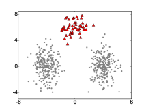
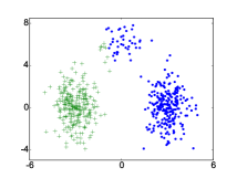
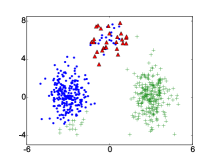
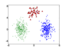
Fig. 1: Synthetic 2D data drawn from two Gaussian distributions. The outliers are represented as the red triangles. (top-left) original data with outliers (top-right) Clustering with K-SVD (bottom-left) Clustering with proposed method with $g(u)=u$. (bottom-right) Clustering with proposed method using the log function.

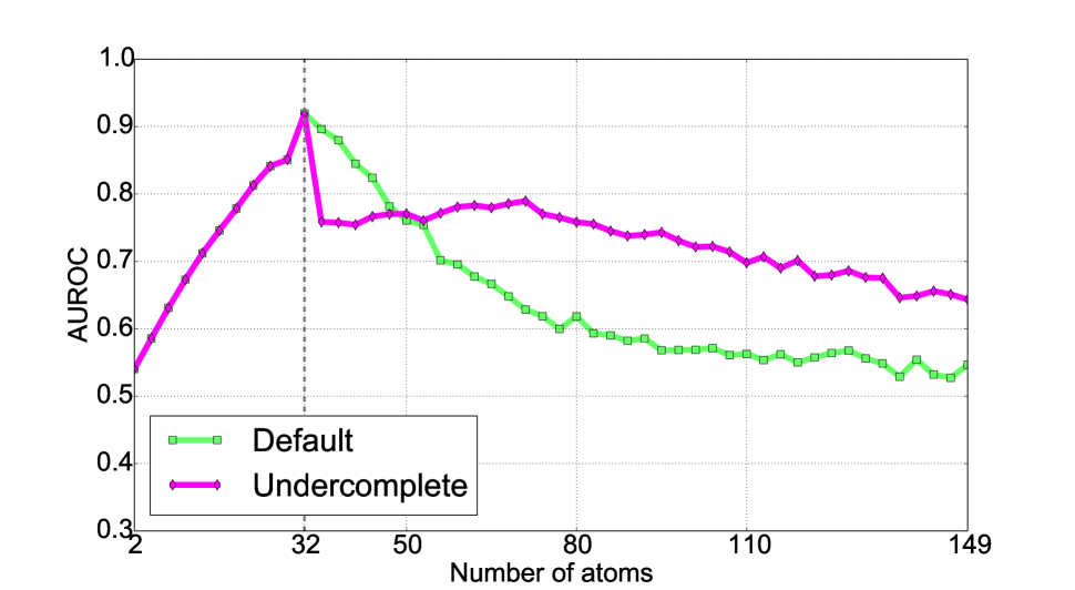
(a) Different dictionary sizes, with 1000 samples and 10% are outliers.

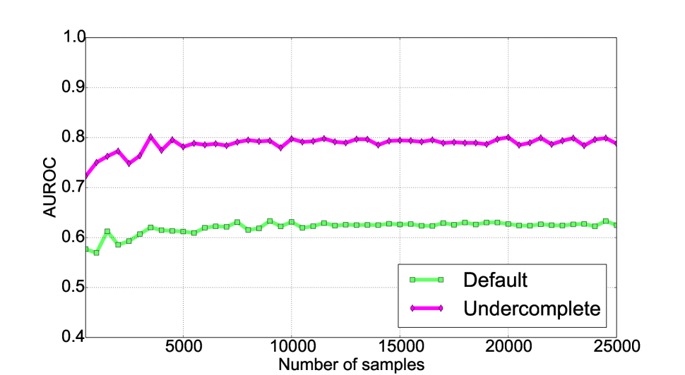
(b) Different number of samples, where 10% are outliers.

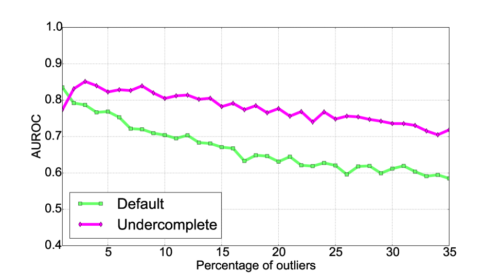
(c) Different outlier ratios (%), with 1000 samples and 64 atoms.

Fig. 2: Performance of the proposed method with multidimensional data.

We use synthetic generated datasets with outliers to demonstrate that our method is robust against outliers. Figure 1 presents two clusters generated from two Gaussian distributions, each containing 250 points along with 50 outliers represented as the red triangles, far away from the clusters. Figure 1 also shows the clustering results using K-SVD [14] as well as the proposed method when $g(u)=u$ and the $log(\epsilon+u)$ functions, respectively. Then, we compare how many of the original outliers are among the 50 highest reconstruction values. The proposed method using the log function proved to be the most robust against outliers, with 47 from the 50 true outliers detected. It is followed by the variant with the identity function, which identified 27 outliers, and finally by K-SVD, which was naturally not able to identify any of the original outliers. This example also shows that concavity of $g$ helps in better identifying outliers.

To further evaluate our proposal, we performed experiments with higher dimensional data (fixed at 32 dimensions). To generate the data, we use the approach described by Lu et al. [15] to create synthetic data based on a dictionary and sparse coefficients. The metric adopted to compare the results is the AUC Curve (AUROC) of outlier scores $\{s_{i}\}$ after running Alg. 1: outliers should have scores $1/s_{i}$ larger than non-outliers, and each point is the average of 5 runs using newly generated data. In Fig. 2a one can observe that the behavior for both lines is the same until the number of atoms reach 32, since $k\leq d$ and the condition in the first line of Alg. 2 is not met. The performance of the undercomplete initialization method also deteriorates for dictionary sizes a little bit greater than $d$, but as far as $k$ starts to increase it becomes evident that this method outperforms the default initialization. Figure 2b shows that our method stays very stable independent of the number of samples, given a constant outlier ratio, regardless of the initialization method. Finally, Fig. 2c shows the behavior of both initialization strategies in scenarios where the outlier proportion changes. It can be noticed that the AUROC values decrease slowly as long as the number of outliers in the samples increase. This is natural since when proportion of outliers is large, outliers can hardly be considered outliers anymore.

3.2 Human attribute classification

In order to prove that our robust dictionary learning method is really beneficial to real data contexts, we also evaluate its performance on the MORPH-II dataset [16], one of the largest labeled face databases available for gender and ethnicity classification, containing more than 40,000 images. Before the training and classification take place, the images are preprocessed, which consists of face detection, align the image based on the eye centers, as well as cropping and resizing. Finally, they are converted to grayscale and SIFT [17] descriptors are computed from a dense grid.

The experiments are run with the proposed method using both the default and the undercomplete initialization approaches using the log function, and then compared with state-of-the-art methods such as K-SVD and LC-KSVD [18]. The classifier uses a Bag of Visual Words (BoVW) approach [19] by replacing the original K-Means algorithm with each of those methods, and then generating a image signature (histogram of frequencies) using the computed clusters, which are later fed to a SVM. This SVM uses a RBF (Radial Basis Function) kernel with tuned $\gamma$ and $C$ parameters. The number of atoms is set to 200 for all experiments.

Method	Ethnicity	Gender
	accuracy	accuracy
Our RDL (default)	96.28	84.76
Our RDL (undercomplete)	96.90	85.79
K-SVD	96.23	81.88
LC-KSVD1	96.24	83.91
LC-KSVD2	95.69	84.69

Table 1: Average classification accuracies (%) for ethnicity and gender classification on the MORPH-II dataset.

Each experiment is the average of 3 runs, each one using 300 selected images per class for training, and the remaining images for classification. The total number of images per class is as follows: 32,874 Africans plus 7,942 Caucasians for ethnicity classification, and 6,799 Females plus 34,017 Males for gender classification. Table 1 shows the overall accuracies. These experiments clearly demonstrate that the quality of the dictionaries computed by the proposed robust dictionary learning method is indeed superior even to methods that uses labels for dictionary learning [18].

4 Conclusions

In this work, we proposed a generic dictionary learning framework which takes advantage of a composition of two concave functions to generate robust dictionaries with very little outlier interference. We also came up with a heuristic initialization which can further increase the identification of outliers, through the use of undercomplete dictionaries. Experiments on synthetic and real world datasets show that the proposed methods outperform some of the state-of-the-art methods such as K-SVD and LC-KSVD, since our approaches are able to achieve higher quality dictionaries which better generalize data.

References

- [1] Michal Aharon, Michael Elad, and Alfred Bruckstein, “-svd: An algorithm for designing overcomplete dictionaries for sparse representation,” IEEE Transactions on signal processing, vol. 54, no. 11, pp. 4311–4322, 2006.
- [2] Julien Mairal, Francis Bach, Jean Ponce, and Guillermo Sapiro, “Online dictionary learning for sparse coding,” in Proceedings of the 26th annual international conference on machine learning. ACM, 2009, pp. 689–696.
- [3] Robert Tibshirani, “Regression shrinkage and selection via the lasso,” Journal of the Royal Statistical Society. Series B (Methodological), pp. 267–288, 1996.
- [4] Francis Bach, Rodolphe Jenatton, Julien Mairal, Guillaume Obozinski, et al., “Optimization with sparsity-inducing penalties,” Foundations and Trends® in Machine Learning, vol. 4, no. 1, pp. 1–106, 2012.
- [5] A Rakotomamonjy, “Applying alternating direction method of multipliers for constrained dictionary learning,” Neurocomputing, vol. 106, pp. 126–136, 2013.
- [6] Feiping Nie, Heng Huang, Xiao Cai, and Chris H Ding, “Efficient and robust feature selection via joint -norms minimization,” in Advances in neural information processing systems, 2010, pp. 1813–1821.
- [7] De Wang, Feiping Nie, and Heng Huang, “Fast robust non-negative matrix factorization for large-scale data clustering,” in 25th International Joint Conference on Artificial Intelligence (IJCAI), 2016, pp. 2104–2110.
- [8] Hua Wang, Feiping Nie, Weidong Cai, and Heng Huang, “Semi-supervised robust dictionary learning via efficient l0-norms minimization,” in Proceedings of the IEEE International Conference on Computer Vision, 2013, pp. 1145–1152.
- [9] Wenhao Jiang, Feiping Nie, and Heng Huang, “Robust dictionary learning with capped l1-norm.,” in IJCAI, 2015, pp. 3590–3596.
- [10] Jianqing Fan and Runze Li, “Variable selection via nonconcave penalized likelihood and its oracle properties,” Journal of the American statistical Association, vol. 96, no. 456, pp. 1348–1360, 2001.
- [11] Cun-Hui Zhang et al., “Nearly unbiased variable selection under minimax concave penalty,” The Annals of statistics, vol. 38, no. 2, pp. 894–942, 2010.
- [12] Ralph Tyrell Rockafellar, Convex analysis, Princeton university press, 2015.
- [13] Varun Chandola, Arindam Banerjee, and Vipin Kumar, “Outlier detection: A survey,” ACM Computing Surveys, 2007.
- [14] Michal Aharon, Michael Elad, and Alfred Bruckstein, “K-svd: An algorithm for designing overcomplete dictionaries for sparse representation,” Signal Processing, IEEE Transactions on, vol. 54, no. 11, pp. 4311–4322, 2006.
- [15] Cewu Lu, Jiaping Shi, and Jiaya Jia, “Online robust dictionary learning,” in Proceedings of the IEEE Conference on Computer Vision and Pattern Recognition, 2013, pp. 415–422.
- [16] Karl Ricanek Jr and Tamirat Tesafaye, “Morph: A longitudinal image database of normal adult age-progression,” in Automatic Face and Gesture Recognition, 2006. FGR 2006. 7th International Conference on. IEEE, 2006, pp. 341–345.
- [17] David G Lowe, “Object recognition from local scale-invariant features,” in Computer vision, 1999. The proceedings of the seventh IEEE international conference on. Ieee, 1999, vol. 2, pp. 1150–1157.
- [18] Zhuolin Jiang, Zhe Lin, and Larry S Davis, “Learning a discriminative dictionary for sparse coding via label consistent k-svd,” in Computer Vision and Pattern Recognition (CVPR), 2011 IEEE Conference on. IEEE, 2011, pp. 1697–1704.
- [19] Gabriella Csurka, Christopher Dance, Lixin Fan, Jutta Willamowski, and Cédric Bray, “Visual categorization with bags of keypoints,” in Workshop on statistical learning in computer vision, ECCV. Prague, 2004, vol. 1, pp. 1–2.