Superadiabatic quantum friction suppression in finite-time thermodynamics

Abstract

Optimal performance of thermal machines is reached by suppressing friction. Friction in quantum thermodynamics results from fast driving schemes that generate nonadiabatic excitations. The far-from-equilibrium dynamics of quantum devices can be tailored by shortcuts to adiabaticity to suppress quantum friction. We experimentally demonstrate friction-free superadiabatic strokes with a trapped unitary Fermi gas as a working substance and establish the equivalence between the superadiabatic mean work and its adiabatic value.

The quest for the optimal performance of thermal machines and efficient use of energy resources has motivated the development of finite-time thermodynamics. At the macroscale, thermodynamic cycles are operated in finite time to enhance the output power, at the expense of inducing friction and reducing the efficiency. Analyzing the tradeoff between efficiency and power has guided efforts in design and optimization CA75 ; FTT84 . The advent of unprecedented techniques to experimentally control and engineer quantum devices at the nanoscale has shifted the focus to the quantum domain. A quantum engine is an instance of a thermal machine in which heat Alicki79 ; Kosloff84 and other quantum resources Scully03 ; Rossnagel14 can be used to produce work. The experimental realization of a single-atom heat engine Rossnagel16 and a quantum absorption refrigerator Maslennikov17 have been demonstrated using trapped ions.

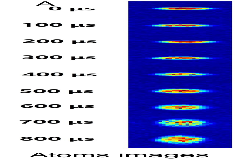
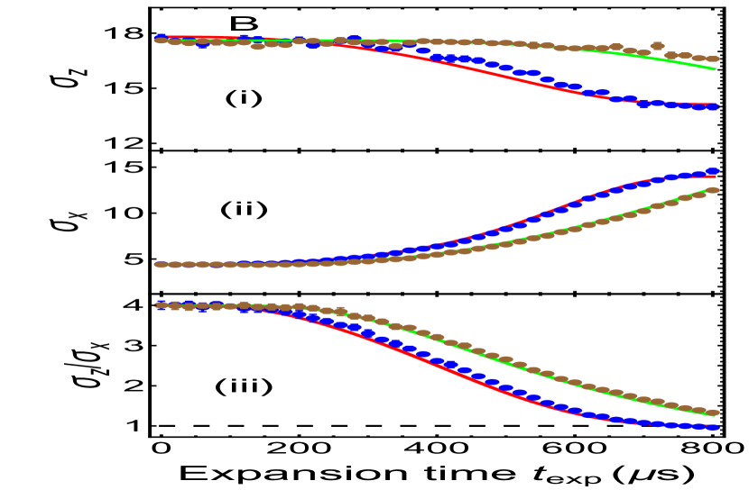
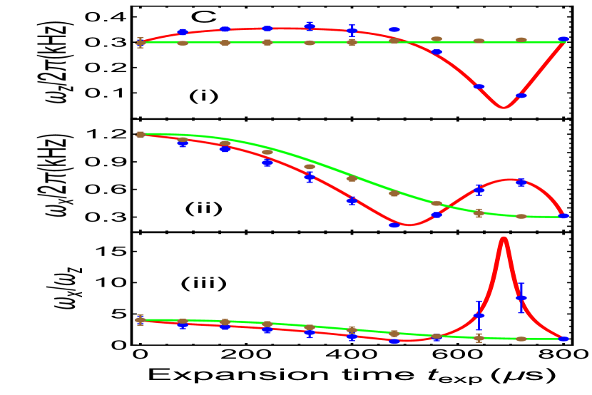
Figure 1: The expansion stroke of the unitary Fermi gas for STA of LCD and reference driving case with $b_{f,x}=4$, keeping $b_{f,y}=b_{f,z}=1$ in $t_{f}=800\mu s$: the atoms images of LCD driving (A), the measured cloud size and cloud aspect ratio (B), and the measured frequencies and frequency aspect ratio (C). Blue dots and brown dots are the measured results for LCD and reference driving case, respectively. The red line and green line are theoretical predictions. The black dashed line denotes for the aspect ratio of 1, indicating an isotropic trap for Fermi gas. Error bars represent the standard deviation of the statistic.

In the quantum domain, the adiabatic theorem Kato50 dictates that excitations are formed during fast driving of the working substance, leading to the emergence of quantum friction. Trading efficiency and power remains a predominant strategy in finite-time quantum thermodynamics, e.g., of ground-state cooling GK92 ; YK06 ; Shiraishi16 . In parallel, new efforts have been devoted to completely suppress friction in finite-time quantum processes. A systematic way of achieving this goal is provided by shortcuts to adiabaticity (STA): fast nonadiabatic processes that reproduce adiabatic dynamics, e.g., in the preparation of a target state STAR . The use of STA provides a disruptive approach in finite-time thermodynamics and has motivated proposals for superadiabatic thermal machines, operating at maximum efficiency and arbitrarily high output power Deng13 ; delcampo14 ; Beau16 ; Abah16 . STA engineering is facilitated by counterdiabatic driving demirplak03 ; Berry09 , whereby an auxiliary control field speeds up the evolution of the system through an adiabatic reference trajectory in a prescheduled amount of time. Experimental demonstrations of counter-diabatic driving have focused on effectively single-particle systems at zero temperature expCD1 ; expCD2 ; expCD3 ; expCD4 . Tailoring excitation dynamics is expected to be a daunting task in complex systems. Yet efficient quantum thermal machines offering scalability require the superadiabatic control of the finite-time thermodynamics in many-particle systems Beau16 . We report the suppression of quantum friction in the finite-time thermodynamics of a strongly-coupled quantum fluid. In our experiment, we implement friction-free superadiabatic strokes with a unitary Fermi gas in an anisotropic time-dependent trap as a working medium.

The unitary regime is reached when the scattering length governing the short-range interactions in a spin-$1/2$ ultracold Fermi gas at resonance greatly surpasses the interparticle spacing. This strongly-interacting state of matter is described by a nonrelativistic conformal field theory DTSon . The controllability of the external trap potential and interatomic interactions in this system allows for the preparation of well-defined many-body states and the precise engineering of time-dependent Hamiltonians. This provides unprecedented opportunities for studying strongly interacting nonequilibrium phenomena BCSBEC . In particular, the emergent scale-invariance symmetry at unitarity facilitates the realization of superadiabatic strokes by the counterdiabatic driving scheme. The work done in a stroke induced by a modulation of the trap frequency can be described by a probability distribution Talkner07 . The mean work equals the difference between the energy of the cloud brought out of equilibrium at the end of the stroke and its initial equilibrium value. Therefore, work done by the cloud is negative while work done on it is positive. For a unitary dynamics, the emergent scaling symmetry at strong coupling anisotropicexpansion dictates the evolution of the nonadiabatic energy in terms of the cloud density profile. The density profile can be characterized using the collective coordinate operators

$$\hat{R}_{x}^{2}=\sum_{i=1}^{N}\hat{x}_{i}^{2},\quad\hat{R}_{y}^{2}=\sum_{i=1}^{N}\hat{y}_{i}^{2},\quad\hat{R}_{z}^{2}=\sum_{i=1}^{N}\hat{z}_{i}^{2}.$$ (1)

Their expectation values determine the shape of the atomic cloud via the scaling factors $b^{2}_{j}(t)=\langle R_{j}^{2}(t)\rangle/\langle R_{j}^{2}(0)\rangle$ in each axis $j=x,y,z$. Their evolution in time is governed by the coupled equations 3DFermi

$$\ddot{b}_{j}(t)+\omega_{j}^{2}(t)b_{j}=\frac{\omega_{j,0}^{2}}{b_{j}\Gamma^{2/3}},\quad j=x,y,z\,,$$ (2)

where $\Gamma=b_{x}(t)b_{y}(t)b_{z}(t)$ is the scaling volume. Under slow driving, the adiabatic scaling factor reads

$$b_{j,ad}(t) =\frac{1}{\Gamma_{ad}^{1/3}}\frac{\omega_{j,0}}{\omega_{j}(t)},$$ (3)

$$\Gamma_{ad}(t) =\prod_{j}b_{j,ad}(t).$$ (4)

In characterizing the finite-time thermodynamics of isolated quantum systems, the ratio of the nonadiabatic and adiabatic mean energies plays a crucial role and is known as the nonadiabatic factor $Q^{*}(t)=\langle\hat{H}(t)\rangle/\langle\hat{H}(t)\rangle_{ad}$ Husimi53 ; Jaramillo16 . For a unitary anisotropic Fermi gas, the nonadiabatic factor is given by (see supplementary text)

$$Q^{*}(t)=\Gamma_{ad}(t)^{2/3}\left[\frac{1}{2\Gamma^{2/3}}+\frac{1}{6}\sum_{j=x,y,z}\frac{\dot{b}_{j}^{2}+\omega_{j}^{2}(t)b_{j}^{2}}{\omega_{j,0}^{2}}\right],$$ (5)

and determines the nonadiabatic mean work

$$\langle W(t)\rangle=(Q^{*}(t)/\Gamma_{ad}^{2/3}(t)-1)\langle H(0)\rangle.$$ (6)

Quantum friction is evidenced during dynamical processes with values of $Q^{*}(t)>1$. To suppress friction, the counterdiabatic driving technique demirplak03 ; Berry09 can be exploited in combination with dynamical scaling laws delcampo13 ; DJD14 to set $Q^{*}=1$. We refer to such superadiabatic control as local counterdiabatic driving (LCD). To implement it, we first identify a desirable reference trajectory of the trap frequencies $\omega_{j}(t)$. We next design a STA protocol with modified frequencies $\Omega_{j}(t)$ that reproduces in an arbitrary prescheduled time $t_{f}$ the final state that would correspond to the adiabatic evolution for $\omega_{j}(t)$. To this end, we choose a reference modulation of the trap, specifically

$$\omega_{j}(t)=\omega_{j}(0)\{1+(b_{f,j}-1)[10\tau^{3}-15\tau^{4}+6\tau^{5}]\},$$ (7)

where $\tau=t/t_{f}$ and $b_{f,j}=\omega_{j}(t_{f})/\omega_{j}(0)$ is set by the ratio of the initial and final target trap frequency. The engineering of a STA by LCD requires the nonadiabatic modulation of the trap frequencies (see supplementary text)

$$\Omega_{j}^{2}(t) =\omega_{j}^{2}-2\left(\frac{\dot{\omega}_{j}}{\omega_{j}}\right)^{2}+\frac{\ddot{\omega}_{j}}{\omega_{j}}+\frac{1}{4}\left(\frac{\dot{\nu}}{\nu}\right)^{2}-\frac{1}{2}\frac{\ddot{\nu}}{\nu}+\frac{\dot{\omega}_{j}\dot{\nu}}{\omega_{j}\nu},$$ (8)

where $\nu(t)=[\omega_{x}(t)\omega_{y}(t)\omega_{z}(t)]^{1/3}$ denotes the geometric mean frequency. The frequencies $\Omega_{j}(t)$ thus satisfy the desired boundary conditions, $\Omega_{j}(0)=\omega_{j}(0)$, $\Omega_{j}(t_{f})=\omega_{j}(t_{f})$, and $\dot{\omega}_{j}(0)=\ddot{\omega}_{j}(t_{f})=0$, while ensuring $Q^{*}(t_{f})=1$. While the LCD dynamics is nonadiabatic at intermediate stages, quantum friction is thus suppressed upon completion of the stroke of arbitrary duration $t_{f}$.

Our experiment probes the nonadiabatic expansion dynamics in an anisotropically-trapped unitary quantum gas, a balanced mixture of ⁶Li fermions in the lowest two hyperfine states $|\!\!\uparrow\rangle\equiv|F=1/2,M_{F}=-1/2\rangle$ and $|\!\!\downarrow\rangle\equiv|F=1/2,M_{F}=1/2\rangle$. The experimental setup is similar to that in Ref. Wu1 ; Wu2 , with a new configuration of the dipole trap consisting in an elliptic beam generated by a cylindrical lens along the $x$-axis and a nearly-ideal Gaussian beam along the $z$-axis (see supplementary text). The resulting potential has a cylindrical symmetry around $x$. This trap facilitates the control of the anisotropy and geometric frequency. Fermionic atoms are loaded into a cross-dipole trap used for evaporative cooling. A Feshbach resonance is used to tune the interactomic interaction to the unitary limit, reached at $B=832\,$G. The system is initially prepared in a stationary state of a normal fluid, with $\omega_{x}(0)=2\pi\times 1200$ Hz and $\omega_{y}(0)=\omega_{z}(0)=2\pi\times 300$ Hz. The initial energy of Fermi gas at unitarity is $E=0.8(0.1)\,E_{F}$, corresponding to a temperature $T=0.25(0.02)\,T_{F}$, where $E_{F}$ and $T_{F}$ are the Fermi energy and temperature of an ideal Fermi gas, respectively.

The time-dependent trap frequencies and trap anisotropy are precisely controlled according to equation (62) for the reference driving, and equation (61) for the LCD driving. To monitor the evolution along the process, after a chosen expansion time with the trap turned on, the trap is completely turned off and the cloud is probed by standard resonant absorption imaging techniques after a time-of-flight expansion time $t_{\rm tof}=600\,\mu s$. Each data point is obtained from averaging $5$ runs of measurements with identical parameters. The time-of-flight density profile along the axial (radial) direction is fitted by a Gaussian function, from which we obtain the observed cloud size $\sigma_{z,\rm obs}$($\sigma_{r,{\rm obs}}$). The in-situ cloud size $\sigma_{z}$ ($\sigma_{r}$) and scaling factors $b_{j}$ during the STA are obtained from the observed value $\sigma_{z,{\rm obs}}$ ($\sigma_{r,{\rm obs}}$) scaled by factor evaluated from the hydrodynamic expansion equation during a time $t_{\rm tof}$ (see supplementary text).

Figure 1 shows the expansion stroke of the unitary Fermi gas with $b_{f,x}=1/4$, $b_{f,y}=b_{f,z}=1$ in $t_{f}=800\mu s$. The trap frequencies are changed from the initial values $\omega_{x}(0)=2\pi\times 1200$ Hz and $\omega_{y}(0)=\omega_{z}(0)=2\pi\times 300$ Hz to the target values $\omega_{x}(t_{f})=2\pi\times 300$ Hz and $\omega_{y}(t_{f})=\omega_{z}(t_{f})=2\pi\times 300$ Hz in 800 $\mu$s. The Fermi gas is initially confined in an anisotropic harmonic trap with a frequency aspect ratio of 4. Due to the engineering of frequencies, the size of the cloud gas is mostly expanded in the $x$ axis, the changes in the $y$ and $z$ directions being small (Fig. 1B) during the driving processes. While the Fermi gas is anisotropic during the nonadiabatic, LCD drive, it becomes isotropic at the final target state, in which both the frequency and cloud size aspect ratio are close to 1; see Fig. 1B(iii) and Fig. 1C(iii).

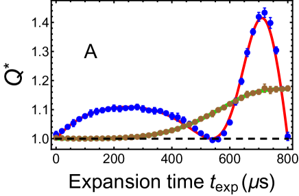
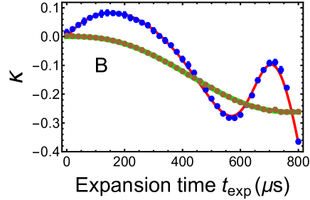
Figure 2: Nonadiabatic factor $Q^{*}$ (A) and the mean work (B) in an expansion stroke. Blue and brown dots denote the measured data for STA of local counter-diabatic driving and nonadiabatic reference driving case while the red and green lines are the corresponding theoretical predictions. $\kappa(t)=\langle W(t)\rangle/\langle\hat{H}(0)\rangle$ is the ratio of the mean work and the initial energy. The black dashed line represents $Q*=1$ where there is no quantum friction. Error bars represent the standard deviation of the statistic.

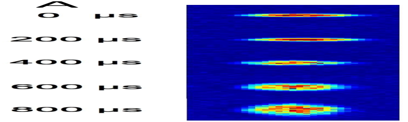
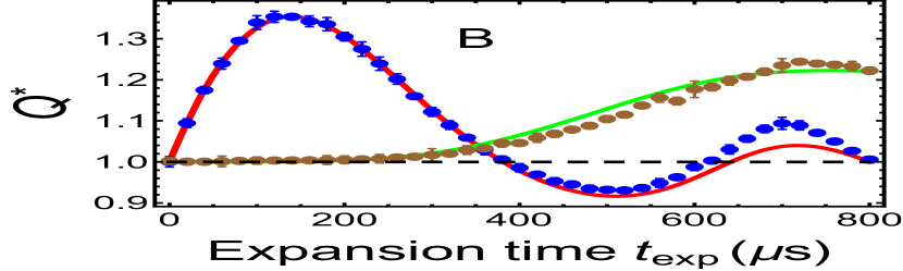
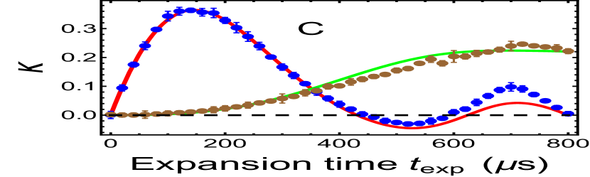
Figure 3: Cloud expansion images (A), nonadiabatic factor $Q^{*}$ (B) and mean work (C) of unitary Fermi gas during a change of the cloud aspect ratio that preserves the geometric mean frequency, $\nu(t_{f})=\nu(0)$. Blue and brown dots represent the measured results for STA of LCD and nonadiabatic driving case, respectively. Red and green lines denote the corresponding theoretical predictions. Black dashed line denotes for the friction-free $Q^{*}(t_{f})=1$ and brown dashed line represents for the zero mean work $\kappa=0$. Error bars represent the standard deviation of the statistic.

The measured nonadiabatic factor $Q^{*}(t)$ and mean work during the expansion stroke are shown in Fig. 6. For the reference driving, the $Q^{*}(t)$ of the strongly interacting Fermi gas monotonically increases, witnessing quantum friction induced by excitations that emerge from the nonadiabatic dynamics. At time $t_{f}=800\mu s$, $Q^{*}(t_{f})$ approaches to 1.17 for the experimental parameters (brown dots in Fig. 6A). Quantum friction decreases the mean work of the stroke, $\kappa(t)=\langle W(t)\rangle/\langle\hat{H}(0)\rangle$ (see Fig. 6B). By contrast, quantum friction is greatly suppressed with the local counterdiabatic driving scheme. Indeed, $Q^{*}(t)$ reduces to 1 after completion of the superadiabatic stroke (blue dots in Fig. 6A), revealing that it is a friction-free process. Using STA by LCD thus allow reaching $Q^{*}(t_{f})=1$, enhancing the work output. Its maximum value is reached at $t_{f}$ and is determined by the geometric mean frequency according to

$$\langle W(t_{f})\rangle_{\rm LCD}=\bigg{(}\bigg{(}\frac{\nu(t_{f})}{\nu(0)}\bigg{)}^{1/3}-1\bigg{)}\langle\hat{H}(0)\rangle.$$ (9)

The measured value of the mean work $\kappa$ in the experiment is about $-0.37$ in units of $\langle\hat{H}(0)\rangle$ (blue dots in Fig. 6B), which is in very good agreement with the theoretical prediction, $(2^{-2/3}-1)=-0.370$. Compared to the case of reference driving process, the mean work in the the local counterdiabatic driving process is increased by nearly 42.3$\%$.

As seen from Eq. 9, in a STA by LCD quantum friction is suppressed and the final mean work depends only on the ratio of geometric mean frequency between the initial state and the target state. For processes satisfying $\nu(t_{f})=\nu(0)$, such as a change of the anisotropy of the cloud, the mean work vanishes. We verify this prediction experimentally. The strongly interacting Fermi gas is first prepared in a quantum state with frequencies of $\omega_{x}(0)=2\pi\times 1200$ Hz and $\omega_{y}(0)=\omega_{z}(0)=2\pi\times 300$ Hz. Then, following by Eq. 62, the trap frequencies are changed to $\omega_{x}(t_{f})=\omega_{y}(t_{f})=\omega_{z}(t_{f})=2\pi\times(\prod_{j}\omega_{j}(0))^{1/3}=2\pi\times 476.22$ Hz, modifying the aspect ratio of the cloud. The measured nonadiabatic factor $Q^{*}(t)$, mean work and cloud expansion images are presented in Fig. 7. It is apparent that there is no friction $Q^{*}(t_{f})=1$ (blue dots in Fig. 7A) and that the mean work vanishes $W(t_{f})=0$ (blue dots in Fig. 7B) when manipulating the quantum state using STA by LCD. For the nonadiabatic reference driving, quantum friction is however induced and causes $Q^{*}(t_{f})>1$ (brown dots in Fig. 7A), signaling energy dispersion in the final state. The mean work is then increased to a positive value of 1.22$\langle\hat{H}(0)\rangle$ (brown dots in Fig. 7B).

A global measure of the nonadiabatic character of a superadiabatic stroke can be quantified by the time-average deviation of the mean work $\langle W(t)\rangle$ from the adiabatic value $\langle W_{ad}(t)\rangle$ as a function of the total time $t_{f}$

$$\delta W=\frac{1}{t_{f}}\int_{0}^{t_{f}}dt\left[\langle W(t)\rangle-\langle W_{ad}(t)\rangle\right].$$ (10)

In the experiment, we measure the mean work deviation in both a STA based on LCD driving and a nonadiabatic reference protocol for the expansion strokes. The initial and final geometric frequencies are fixed to $4.8$ and $1.2$, respectively. The trap frequencies are changed from the initial frequencies $\omega_{x}=2\pi\times 1440$ Hz, $\omega_{y}=\omega_{z}=2\pi\times 300$ Hz to $\omega_{x}=2\pi\times 360$ Hz, $\omega_{y}=\omega_{z}=2\pi\times 300$ Hz in different time $t_{f}$. For STA by LCD driving, the mean work $\langle W(t_{f})\rangle$ does not change no matter how short the time $t_{f}$ is. However, $\langle W(t)\rangle$ at $t<t_{f}$ keeps changing to reflect how large the excess work needed to implement STA at different stages. The measured results are shown in Fig. 8. The shorter the time $t_{f}$, the greater the deviation of mean work $\delta W$. The solid curves are the fits with a power-law $1/t_{f}^{2}$ as a function of the duration of the stroke $t_{f}$.

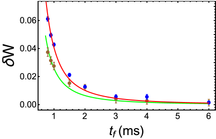
Figure 4: Time-averaged mean work deviation $\delta W$ in units of $\langle H(0)\rangle$ as a function of $t_{f}$. Blue and brown dots denote the measured data for STA by LCD driving and the nonadiabatic reference driving case, while the red and green lines are the fits with a function of $1/t_{f}^{2}$. Error bars represent the standard deviation of the measurement data.

The experiments presented here demonstrate the suppression of quantum friction and enhancement of the mean work output in superadiabatic strokes with a strongly interacting quantum fluid as a working medium. The control of the finite-time quantum thermodynamics is achieved using shortcuts to adiabaticity that exploit the emergent scale-invariance of a unitary Fermi gas. In combination with cooling and heating steps, superadiabatic strokes can be used to engineer quantum heat engines Deng13 ; delcampo14 ; Beau16 ; Salamon09 ; Abah16 and refrigerators Rezek09 ; Stefanatos10 ; Hoffmann11 , e.g., based on a quantum Otto cycle, that operate at maximum efficiency with high output and cooling power.

Acknowlegments.— This research is supported by the National Key Research and Development Program of China (grant no.2017YFA0304201), National Natural Science Foundation of China (NSFC) (grant nos. 11374101 and 91536112), Program of Shanghai Subject Chief Scientist(17XD1401500), UMass Boston (project P20150000029279) and the John Templeton Foundation.

I Supplemental Material

II Finite-time thermodynamics of a unitary Fermi gas in a time-dependent anisotropic trap

The Hamiltonian of a unitary Fermi gas confined in a 3D anisotropic harmonic trap whose frequency is time dependent is given by

$$\hat{H}(t)=\sum_{i=1}^{N}\left[-\frac{\hbar^{2}}{2m}\nabla_{i}^{2}+\frac{1}{2}m\left(\omega_{x}^{2}(t)x_{i}^{2}+\omega_{y}^{2}(t)y_{i}^{2}+\omega_{z}^{2}(t)z_{i}^{2}\right)\right]+\sum_{i<j}U({\bf r}_{i}-{\bf r}_{j}),$$ (11)

where $\omega_{j}$ ($j=x,y,z$) is the corresponding trapping frequency along the $j$-axis. The short-range pair-wise interaction potential becomes a homogeneous function of degree $-2$ in the unitary limit, satisfying

$$U(\lambda{\bf r})=\frac{1}{\lambda^{2}}U({\bf r}).$$ (12)

In what follows it is convenient to rewrite the total hamiltonian $\hat{H}(t)$ as the sum

$$\hat{H}(t)=\hat{H}_{0}+\hat{H}_{\rm trap}(t),$$ (13)

where

$$\hat{H}_{0} = \sum_{i=1}^{N}\left(-\frac{\hbar^{2}}{2m}\nabla_{i}^{2}\right)+\sum_{i<j}U(\mathbf{r}_{i}-\mathbf{r}_{j}),$$ (14)

$$\hat{H}_{\rm trap}(t) = \frac{1}{2}m\sum_{i=1}^{N}\left[\omega_{x}^{2}(t)x_{i}^{2}+\omega_{y}^{2}(t)y_{i}^{2}+\omega_{z}^{2}(t)z_{i}^{2}\right].$$ (15)

For an exact treatment of the finite-time thermodynamics we compute the nonadiabatic evolution of the mean work. To this end, we note that

$$\frac{d}{dt}\hat{H}_{0} = \frac{1}{i\hbar}\left[\hat{H}_{0},\hat{H}(t)\right]$$ (16)

$$= \frac{1}{i\hbar}\left[\hat{H}(t)-\hat{H}_{\rm trap}(t),\hat{H}(t)\right]$$ (17)

$$= -\frac{1}{2}m\sum_{i=1}^{N}\left(\omega_{x}^{2}(t)\frac{d\hat{x}_{i}^{2}}{dt}+\omega_{y}^{2}(t)\frac{d\hat{y}_{i}^{2}}{dt}+\omega_{z}^{2}(t)\frac{d\hat{z}_{i}^{2}}{dt}\right).$$ (18)

We introduce the collective coordinate operators

$$\hat{R}_{x}^{2}=\sum_{i=1}^{N}\hat{x}_{i}^{2},\quad\hat{R}_{y}^{2}=\sum_{i=1}^{N}\hat{y}_{i}^{2},\quad\hat{R}_{z}^{2}=\sum_{i=1}^{N}\hat{z}_{i}^{2},$$ (19)

and define via their expectation values the scaling factors

$$b_{j}(t)=\left[\frac{\langle\hat{R}_{j}^{2}(t)\rangle}{\langle\hat{R}_{j}^{2}(0)\rangle}\right]^{1/2},\quad j=x,y,z.$$ (20)

For an equilibrium state, we use Hellman-Feyman theorem and the scaling property of the Hamiltonian to find

$$\langle\hat{R}_{j}^{2}(0)\rangle=\frac{1}{3m\omega_{j,0}^{2}}\langle\hat{H}(0)\rangle,\quad j=x,y,z.$$ (21)

The expectation value of Eq. (18) can thus be written as

$$\frac{d}{dt}\langle\hat{H}_{0}\rangle = -\frac{1}{2}m\sum_{j=x,y,z}\omega_{j}^{2}(t)\frac{d\langle R_{j}^{2}(t)\rangle}{dt}$$ (22)

$$= -\frac{1}{6}\sum_{j=x,y,z}\frac{\omega_{j}^{2}(t)}{\omega_{j,0}^{2}}\frac{db_{j}^{2}}{dt}\langle\hat{H}(0)\rangle$$ (23)

$$= -\frac{1}{3}\sum_{j=x,y,z}\frac{\omega_{j}^{2}(t)}{\omega_{j,0}^{2}}b_{j}\dot{b}_{j}\langle\hat{H}(0)\rangle.$$ (24)

For a 3D unitary Fermi gas, the scaling factors are coupled via the evolution equations

$$\ddot{b}_{j}+\omega_{j}^{2}(t)b_{j}=\frac{\omega_{j,0}^{2}}{b_{j}\Gamma(t)^{2/3}},\quad j=x,y,z,$$ (25)

where the volume scaling factor is given by $\Gamma(t)=\prod_{j}b_{j}(t)$.

Combining (25) and (24), we rewrite the rate of change of the expectation value of $\hat{H}_{0}$ as

$$\frac{d}{dt}\langle\hat{H}_{0}\rangle = \frac{1}{3}\sum_{j=x,y,z}\left(\frac{\dot{b}_{j}\ddot{b}_{j}}{\omega_{j,0}^{2}}-\frac{\dot{b}_{j}}{b_{j}\Gamma^{2/3}}\right)\langle\hat{H}(0)\rangle$$ (26)

$$= \frac{d}{dt}\left(\frac{1}{2\Gamma^{2/3}}+\frac{1}{6}\sum_{j=x,y,z}\frac{\dot{b}_{j}^{2}}{\omega_{j,0}^{2}}\right)\langle\hat{H}(0)\rangle.$$ (27)

As for the variation of the expectation value of the trapping potential term, it simply reads

$$\frac{d}{dt}\langle\hat{H}_{\rm trap}(t)\rangle = \frac{d}{dt}\left(\frac{1}{6}\sum_{j=x,y,z}\frac{\omega_{j}^{2}(t)}{\omega_{j,0}^{2}}b_{j}^{2}\right)\langle\hat{H}(0)\rangle.$$ (28)

The exact expression for the nonadiabatic mean energy directly follows from integrating the differential equation

$$\frac{d}{dt}\langle\hat{H}\rangle=\frac{d}{dt}\langle\hat{H}_{0}+\hat{H}_{\rm trap}(t)\rangle,$$ (29)

with the boundary condition $\langle\hat{H}(t=0)\rangle=\langle\hat{H}(0)\rangle$ and reads

$$\langle\hat{H}(t)\rangle=\left[\frac{1}{2\Gamma^{2/3}}+\frac{1}{6}\sum_{j=x,y,z}\frac{\dot{b}_{j}^{2}+\omega_{j}^{2}(t)b_{j}^{2}}{\omega_{j,0}^{2}}\right]\langle\hat{H}(0)\rangle,$$ (30)

which is the central result of this section, from which all finite-time thermodynamics can be derived.

In the adiabatic limit under slow driving, the scaling factors remain coupled and fulfill

$$b_{j,ad}(t)=\frac{1}{\Gamma_{ad,t}^{1/3}}\frac{\omega_{j,0}}{\omega_{j}(t)},\quad{\rm where}\quad\Gamma_{ad}(t)=\prod_{j}b_{j,ad}(t).$$ (31)

Therefore, the instantaneous adiabatic mean energy reads

$$\langle\hat{H}(t)\rangle_{ad}=\frac{1}{\Gamma_{ad}^{2/3}}\langle\hat{H}(0)\rangle.$$ (32)

The ratio between the nonadiabatic and adiabatic mean energies plays a crucial role in finite-time thermodynamics and is known as the the nonadiabatic factor Husimi53 ; Jaramillo16

$$Q^{\ast}(t)=\langle\hat{H}(t)\rangle/\langle\hat{H}(t)\rangle_{ad},$$ (33)

that quantifies quantum friction. For a unitary Fermi gas, the nonadiabatic factor and mean work read

$$Q^{*}(t) =\Gamma_{ad}^{2/3}\left[\frac{1}{2\Gamma^{2/3}}+\frac{1}{6}\sum_{j=x,y,z}\frac{\dot{b}_{j}^{2}+\omega_{j}^{2}(t)b_{j}^{2}}{\omega_{j,0}^{2}}\right],$$ (34)

$$\langle W(t)\rangle =\langle H(t)\rangle-\langle H(0)\rangle=\left[\frac{1}{2\Gamma^{2/3}(t)}+\frac{1}{6}\sum_{j=x,y,z}\frac{\dot{b}_{j}^{2}+\omega_{j}^{2}(t)b_{j}^{2}}{\omega_{j,0}^{2}}-1\right]\langle\hat{H}(0)\rangle.$$ (35)

II.1 Local counterdiabatic control of the finite-time thermodynamics of a unitary Fermi gas

An arbitrary modulation in time of the trapping potential generally induces a nonadiabatic evolution. We aim at tailoring excitations to control the finite-time thermodynamics of the system. This goal is at reach using techniques known as shortcuts to adiabaticity. Specifically, the counterdiabatic driving technique demirplak03 ; Berry09 can be exploited in combination with dynamical scaling laws to control the nonadiabatic dynamics of many-body quantum systems as discussed in delcampo11 ; delcampo13 ; DJD14 .

Our approach to achieve superadiabatic control relies on first designing a desirable reference trajectory by specifying the modulation of the parameters of the Hamiltonian, i.e., $\omega_{j}(t)$. Subsequently, we consider an alternative protocol with frequencies $\omega_{j}(t)\rightarrow\Omega_{j}(t)$ that lead to the same final state than the adiabatic evolution corresponding to $\omega_{j}(t)$. The modified protocol with trap frequencies $\Omega_{j}(t)$ can be found for an arbitrary value $t_{f}$ of the duration of the stroke, provided that $\Omega_{j}(t)$ can be implemented.

To design the reference evolution of the cloud, let $\{\omega_{j,0}|j=x,y,z\}$ denote the frequencies of the anisotropic harmonic trap at $t=0$. Similarly, let $\{b_{j,f}|j=x,y,z\}$ denote the target scaling factors upon completion of an expansion or compression stroke of duration $t_{f}$. Imposing the following boundary conditions

$$\omega_{j}(0) = \omega_{j,0},~{}~{}~{}\omega_{j}(t_{f})=b_{j,f}^{-2}\omega_{j}(0),$$ (36)

$$\dot{\omega}_{j,0} = 0,~{}~{}~{}~{}~{}~{}\dot{\omega}_{j,f}=0,$$ (37)

$$\ddot{\omega}_{j,0} = 0,~{}~{}~{}~{}~{}~{}\ddot{\omega}_{j,f}=0,$$ (38)

we determine a possible choice for the time-dependent scaling factors via the polynomial ansatze $\omega_{j}(t)=\omega_{j,0}\sum_{n}c_{n}(t/t_{f})^{n}$. Specifically,

$$\omega_{j}(t)=\omega_{j,0}\left[1+10\left(b_{j,f}^{-2}-1\right)\left(\frac{t}{t_{f}}\right)^{3}-15\left(b_{j,f}^{-2}-1\right)\left(\frac{t}{t_{f}}\right)^{4}+6\left(b_{j,f}^{-2}-1\right)\left(\frac{t}{t_{f}}\right)^{5}\right].$$ (39)

Consistently, the reference expansion factor is set by the adiabatic consistency equations

$$b_{j}(t) =\frac{\omega_{j,0}}{\omega_{j}(t)\Gamma_{ad}^{1/3}(t)}$$ (40)

$$=\frac{\omega_{j,0}}{\omega_{j,t}}\left[\frac{\nu(t)}{\nu(0)}\right]^{1/2},$$ (41)

where the geometric mean frequency equals $\nu(t)=[\omega_{x}(t)\omega_{y}(t)\omega_{z}(t)]^{1/3}$.

The above equations describe the evolution of the scaling factors in the adiabatic limit under slow driving. Nonetheless, they describe as well the exact nonadiabatic dynamics under a modified driving protocol with a different time-dependence of the trapping frequencies, i.e., replacing $\omega_{j}(t)\rightarrow\Omega_{j}(t)$, where the explicit form of $\Omega_{j}(t)$ is to be determined. This approach, generally referred to as local counterdiabatic driving (LCD), has been discussed for the single-particle time-dependent harmonic oscillator and many-body quantum systems in one spatial dimension and under isotropic confinement in higher dimensions delcampo11 ; delcampo13 ; DJD14 . For a unitary Fermi gas in a 3D anisotropic trap, the requiring driving frequencies are given by

$$\Omega_{j}^{2}(t) =\frac{\omega_{j,0}^{2}}{b_{j}^{2}\Gamma^{2/3}}-\frac{\ddot{b}_{j}}{b_{j}}$$ (42)

$$=\omega_{j}^{2}(t)-\frac{\ddot{b}_{j}}{b_{j}}\ ,$$ (43)

where $b_{j}(t)$ are given by Eqs. (40). The explicit expression for $\Omega_{j}^{2}(t)$ reads

$$\Omega_{j}^{2}(t) = \omega_{j}^{2}-2\left(\frac{\dot{\omega}_{j}}{\omega_{j}}\right)^{2}+\frac{\ddot{\omega}_{j}}{\omega_{j}}-\frac{4}{9}\left(\frac{\dot{\Gamma}}{\Gamma}\right)^{2}+3\frac{\ddot{\Gamma}}{\Gamma}-\frac{2}{3}\frac{\dot{\omega}_{j}\dot{\Gamma}}{\omega_{j}\Gamma}$$ (44)

$$= \omega_{j}^{2}-2\left(\frac{\dot{\omega}_{j}}{\omega_{j}}\right)^{2}+\frac{\ddot{\omega}_{j}}{\omega_{j}}+\frac{3}{4}\left(\frac{\dot{\nu}}{\nu}\right)^{2}-\frac{1}{2}\frac{\ddot{\nu}}{\nu}+\frac{\dot{\omega}_{j}\dot{\nu}}{\omega_{j}\nu}\,,$$ (45)

which includes counterdiabatic corrections arising from $\omega_{j}$, the geometric mean $\nu$, and their coupling. The nonadiabatic factor for a unitary Fermi gas under local counterdidabatic driving reads

$$Q^{*}(t) = 1+\frac{1}{6}\Gamma(t)^{2/3}\sum_{j}\frac{\dot{b}_{j}^{2}-b_{j}\ddot{b}_{j}}{\omega_{j,0}^{2}}$$ (46)

$$= 1+\frac{1}{6}\sum_{j}\left(\frac{\ddot{\omega}_{j}}{\omega_{j}^{3}}-\frac{\dot{\omega}_{j}^{2}}{\omega_{j}^{4}}-\frac{\ddot{\nu}}{2\nu\omega_{j}^{2}}+\frac{\dot{\nu}^{2}}{2\nu^{2}\omega_{j}^{2}}\right).$$ (47)

When the scaling factors are isotropic so that $b_{j}(t)=b(t)$, the axis subindex $j$ can be dropped out, the volume scaling factor simplifies to $\Gamma(t)=b(t)^{3}=[\omega_{0}/\omega(t)]^{\frac{3}{2}}$ and

$$\Omega^{2}(t)=\omega^{2}(t)-\frac{3}{4}\left[\frac{\dot{\omega}(t)}{\omega(t)}\right]^{2}+\frac{1}{2}\frac{\ddot{\omega}(t)}{\omega(t)}\ ,$$ (48)

in agreement with  delcampo13 ; DJD14 . Similarly, in the isotropic case the nonadiabatic factor reduces to

$$Q^{*}(t)=1+\frac{1}{4}\left(\frac{\ddot{\omega}}{\omega^{3}}-\frac{\dot{\omega}^{2}}{\omega^{4}}\right),$$ (49)

which agrees for the result in one-dimensional harmonically trapped systems Beau16 ; Abah17 .

III Experiment methods

The experimental setup is similar to that described in our previous work Wu1 ; Wu2 . We realize a large atom-number magneto-optical trap (MOT) by employing a laser system of 2.5-watts laser output with Raman fiber amplifier and intracavity frequency-doubler. When the MOT loading and cooling stage are finished, an optical pumping process is performed and a balanced mixture of atoms in the two lowest hyperfine states, $|\!\!\uparrow\rangle\equiv|F=1/2,M_{F}=-1/2\rangle$ and $|\!\!\downarrow\rangle\equiv|F=1/2,M_{F}=1/2\rangle$, is prepared.

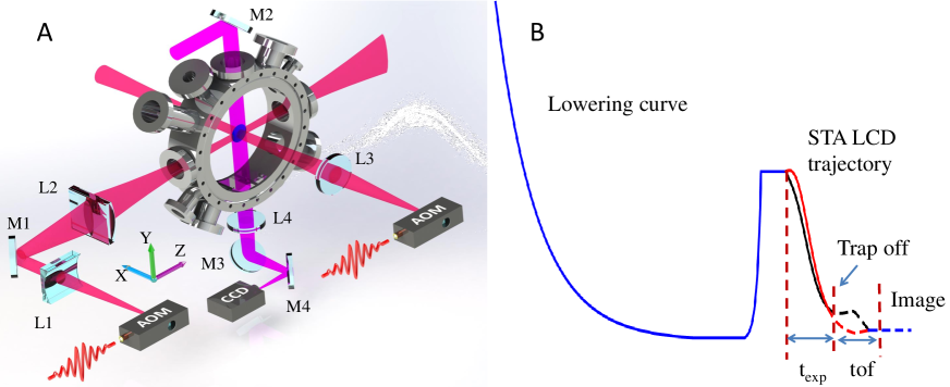
Figure 5: Schematic of the experimental setup (A) and the experimental procedure (B). A specially designed optical crossed-dipole trap is formed by two orthogonal far-off resonance laser beams, providing a highly controllable trap frequency. M1-M4, Mirrors; L1-L2, cylindrical lenes; L3-L4, achromatic lenses; AOM, acousto-optic modulator; tof, time-of-flight.

After the MOT stage, the atoms are first loaded into an optical dipole trap formed by a single beam. A forced evaporation is performed to cool atoms to quantum degeneracy in an external magnetic field at 832 G. Two seconds later a specially designed optical crossed dipole trap is switched on and nearly $10^{5}$ atoms are transferred to this trap. Further forced evaporation is implemented by slightly reducing the power of the two orthogonal beams. In this way, the system is initially prepared in a stationary state with a dimensionless temperature $T/T_{F}\approx 0.25$, where $T_{F}$ is the Fermi temperature. Subsequently, we start the STA experiment based on LCD, schematically described in Fig. 5B. After the evolved time $t_{exp}$, the beams of the crossed dipole trap are switched off and an absorption image is taken with the time of flight.

The specially-designed optical dipole trap, which consists of two orthogonal far-off resonance laser beams, provides a flexible control of the trap frequencies, as is shown in Fig. 5A. The first beam propagates along the $z$-axis, i.e., the horizontal direction. The beam is focused by a pair of cylindrical lens, which cause the more tight confinement in the $x$ direction. The Gaussian waists are 42 $\mu$m along the $x$-axis and about 1200 $\mu$m in the $y$ direction. The second beam, perpendicular to the first, propagates along the $x$ direction, i.e. the vertical beam. The beam has a nearly perfect Gaussian profile, with a waist of $\approx$ 68 $\mu$m, which provides both strong confinement in the $y$ and $z$ directions. Therefore, the frequency in the $x$ direction mostly depends on the power of the horizontal beam while the vertical beam determines the frequencies both in the $y$ and $z$ directions. The frequency aspect ratio of the trap can be simply controlled by precisely adjusting the power ratio of the two beams.

IV Expansion factor

The dynamics of the system is investigated by measuring the radius of the atomic cloud. At different stages of the superadiabatic stroke, an absorption image is taken after releasing the atomic cloud in a time-of-flight expansion. The observed cloud size can be related to cloud size inside the trap, by accounting for the time-of-flight expansion scaling factor $b_{j}$ along each axis ($j=x,y,z$). The time-of-flight density profile along each direction is fitted by a Gaussian function as $A_{0}+A_{1}e^{-r_{j}^{2}/\sigma_{j}^{2}}$ in the normal fluid regime. From this fit we obtain the observed cloud size $\langle\sigma_{j}\rangle_{obs}$. $\langle\sigma_{j}\rangle_{obs}$ is related to the in situ cloud size via $\langle\sigma_{j}\rangle=\langle\sigma_{j}\rangle_{obs}/b_{j}$. Because $\sigma_{j}$ is obtained by a Gaussian fit to the density profile, $\langle\sigma_{j}^{2}\rangle=2\langle R_{j}^{2}\rangle$, and thus the expansion dynamics can be monitored by directly measuring the density profile.

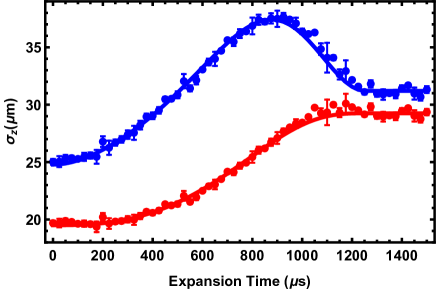
Figure 6: Determination of the cloud size $\langle\sigma_{z}\rangle$ obtained from the Gaussian fit of the density profile of the unitary Fermi gas for a time-of-flight $t_{tof}=600\,\mu$s. The blue dots are the data $\langle\sigma_{z}\rangle_{obs}$ and the red dots are $\langle\sigma_{z}\rangle=\langle\sigma_{z}\rangle_{obs}/b_{tof}$. The red solid line is the best fit based on theory curve. The blue solid line is the red solid line multiplied by $b_{tof}$. Error bars represent the standard deviation of the statistics.

To analyze the measurements we use the equations of motion for the scaling factors of a unitary Fermi gas

$$\ddot{b}_{j}+\omega_{j}^{2}(t)b_{j}=\frac{\omega_{j,0}^{2}}{b_{j}\Gamma^{2/3}}\ ,~{}~{}~{}j=x,y,z~{}$$ (50)

where $b_{j}$ denotes the expansion scaling factor in $j$ direction and $\omega_{j,0}$ is the initial frequency measured by the parametric resonance for the atomic cloud. During the local counterdiabatic driving of the system, the time-dependent frequencies are given by

$$\omega_{j}(t)=\left\{\begin{aligned} \Omega_{j}(t),~{}~{}~{}t_{0}<&t\leq t^{\prime}\\ 0,~{}~{}~{}t^{\prime}<&t\leq t^{\prime}+t_{tof}\end{aligned}\right.$$ (51)

Here $t_{0}$ is the time when we start the STA process, $t^{\prime}=t_{0}+t_{exp}$ is the time at which we turn off the trap, and $t_{tof}$ is the duration of the time-of-flight expansion for imaging of the cloud. Using equations (50) and (51), we can numerically calculate the expansion factors at any time $t$ using the boundary conditions $b_{j}(t_{0})=1$ and $\dot{b}_{j}(t_{0})=0$ for all $j=x,y,z$. In Fig. 6, we show $\langle\sigma_{z}\rangle$ and $\langle\sigma_{z}\rangle_{obs}$ of the unitary Fermi gas for a time-of-flight $t_{tof}=600\mu$s.

V Expansion and compression stroke

A quantum Otto cycle consists of a sequence of four strokes, with isentropic and isochoric strokes alternating with each other KR17 ; Beau16 . We focus on the implementation of the isentropic expansion and the compression strokes during which the dynamics is unitary. Utilizing STA based on LCD driving, we implement the superadiabatic variants of the expansion and compression strokes with a 3D unitary Fermi gas as a working medium. Experimentally, we consider two different trap configurations, associated with the end points of the expansion and compression stages. The corresponding trap frequencies are

$$\Phi_{1} :~{}~{}~{}~{}~{}~{}\omega_{x1}=2\pi\times 1600~{}\text{Hz},~{}~{}~{}~{}\omega_{y1}=\omega_{z1}=2\pi\times 200~{}\text{Hz},$$ (52)

$$\Phi_{2} :~{}~{}~{}~{}~{}~{}\omega_{x2}=2\pi\times~{}400~{}~{}\text{Hz},~{}~{}~{}~{}\omega_{y2}=\omega_{z2}=2\pi\times 200~{}\text{Hz}.$$ (53)

The energies of the corresponding quantum states $\Phi_{1}$ and $\Phi_{2}$, are denoted by $\langle H_{1}\rangle$ and $\langle H_{2}\rangle$, respectively. The expansion stroke is performed from state $\Phi_{1}$ to state $\Phi_{2}$ and the compression stroke is manipulated by reversing the expansion procedure. The frequencies of the two strokes have the following relations,

$$\Omega_{j,exp}(0) =\omega_{j,1},~{}~{}~{}~{}~{}\Omega_{j,exp}(t_{f})=\omega_{j,2},~{}~{}~{}~{}~{}\Omega_{j,exp}(t)=\Omega_{j,1}(t),$$ (54)

$$\Omega_{j,comp}(0) =\omega_{j,2},~{}~{}~{}\Omega_{j,comp}(t_{f})=\omega_{j,1},~{}~{}~{}\Omega_{j,comp}(t)=\Omega_{j,1}(t_{f}-t),$$ (55)

where $\Omega_{j,exp}$ and $\Omega_{j,comp}$ are the frequencies for the expansion and compression strokes, respectively.

Along the expansion stroke, the aspect ratio is initially fixed to be 8 and finally reaches the value 2 at time $t_{f}$. The reverse processes associated with the compression stroke thus changes the trap frequency aspect ratio from 2 to 8.

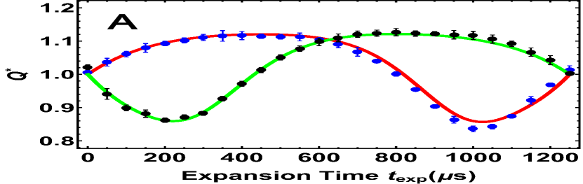
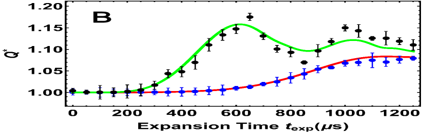
Figure 7: The evolution of the non-adiabatic factor $Q^{*}(t)$ for the expansion and compression strokes. (A) $Q^{*}(t)$ for STA with LCD driving. (B) $Q^{*}(t)$ for the reference driving. For both (A) and (B), blue dots and black dots represent measurement data for the expansion and compression strokes, respectively, while the red line and green line are the corresponding theoretical predictions. Error bars represent the standard deviation of the measurement statistics.

The measured results for the non-adiabatic factor $Q^{*}(t)$ are shown in Fig. 7. The non-adiabatic factor of both the expansion and compression strokes for LCD driving go back to 1 at the time $t=t_{f}$, showing that there are frictionless, i.e., satisfying $Q^{*}(t_{f})=1$. By contrast, the reference driving exhibits friction with values of $Q^{*}(t_{f})$ greater than unity. Therefore, we demonstrate that a STA protocol by LCD driving of a unitary Fermi gas is not only suitable for an expansion stroke, but also for its superadiabatic compression in finite time. Based on this fast driving scheme, one can induce frictionless control so as to transfer strongly interacting fluids between thermal equilibrium states.

Note that while in a STA energy excitations are transient and they vanish upon completion of the stroke, there are large energy excitations for the compression stroke of the nonadiabatic reference driving process in the final state $t=t_{f}$. The shear viscosity can not be neglected at the high energy of unitary Fermi gas Thomas1 ; Thomas2 and we take it into consideration for the theoretical calculations of the reference driving of the compression stroke in Fig. 7.

The mean work for the LCD driving is determined by the geometric frequency according to equation (15). The theoretical mean work is therefore

$$\langle W_{exp}(t_{f})\rangle =(1/\Gamma_{exp,ad}^{2/3}(t_{f})-1)\langle H(0)\rangle_{1},$$ (56)

$$\langle W_{comp}(t_{f})\rangle =(1/\Gamma_{comp,ad}^{2/3}(t_{f})-1)\langle H(0)\rangle_{2},$$ (57)

where $\langle H(0)\rangle_{1}$ and $\langle H(0)\rangle_{2}$ are the equilibrium mean energies of the states $\Phi_{1}$ and $\Phi_{2}$, respectively. Given that the adiabaticity condition is fulfilled upon completion of the adiabatic and superadiabatic strokes, one finds that

$$\langle W_{exp}(t_{f})\rangle+W_{comp}(t_{f})=0,$$ (58)

$$\Gamma_{exp,ad}(t_{f})=1/\Gamma_{comp,ad}(t_{f}).$$ (59)

To characterize the evolution of the mean work, we define the dimensionless factor $\kappa$ as

$$\kappa=\langle W(t)\rangle/\langle H(0)\rangle.$$ (60)

Fig. 8 shows the evolution of $\kappa$ for both the expansion and compression strokes. The energy of the evolving state in the expansion process decreases and is below its initial vale, therefore $\kappa$ acquires negative values. However, the energy in the compression process is increased and $\kappa$ is positive. Upon completion of the stroke, the mean work for the reference driving is always larger than the one for the corresponding LCD driving, indicating that an excess energy is added for nonadiabatic driving over the adiabatic value. This excess of energy results from the existence of friction for the reference driving. In a thermodynamic cycle, friction in the strongly interacting quantum fluids would generate excess excitations, reducing the efficiency of the output power for the heating engine.

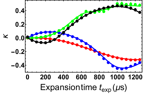
Figure 8: Mean work $\kappa=\langle W(t)\rangle/\langle H(0)\rangle$, for both the expansion stroke and compression stroke. Blue and red dots represent measured data for the expansion stroke while black and green dots are measured results for the compression stroke. Solid lines correspond to the theoretical predictions of the LCD and reference protocols. Error bars represent the standard deviation of the statistics.

In the following, we consider the adiabatic “slow” driving case, where the quantum states are stationary at any time and can be reversed. The mean work for the the expansion and compression strokes can be written as,

$$\int_{0}^{t}dW_{exp}(t)=-\int_{tf-t}^{t_{f}}dW_{comp}(t) =-\langle W_{comp}(t_{f})\rangle+\int_{0}^{t_{f}-t}dW_{comp}(t),$$ (61)

$$\langle W_{exp}(t_{f})\rangle =-\langle W_{comp}(t_{f})\rangle.$$ (62)

Combining Eq. (61) and Eq. (62), we find

$$\langle W_{exp}(t)\rangle-\langle W_{comp}(t_{f}-t)\rangle-\langle W_{exp}(t_{f})\rangle=0.$$ (63)

Here we define another dimensionless factor $\bar{\kappa}=(\langle W_{exp}(t)\rangle-\langle W_{comp}(t_{f}-t)\rangle)/\langle H(0)\rangle_{1}-1$, which denotes the deviation from the adiabatic evolution. The factor $\bar{\kappa}$ should be zero at any time for the real adiabatic process. The measured results are presented in Fig. 9. It shows that $\bar{\kappa}$ for LCD driving is closed to zero, indicating the counter-adiabatic following of the adiabatic trajectory. By contrast, for the reference driving deviations from zero value are clearly observed.

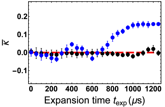
Figure 9: Time evolution of the dimensionless factor $\bar{\kappa}$ for both the expansion and compression strokes, $\bar{\kappa}=(\langle W_{exp}(t)\rangle-\langle W_{comp}(t_{f}-t)\rangle)/\langle H(0)\rangle_{1}-1$. Black and blue dots correspond to the measured data for LCD and reference driving, respectively. The red dashed line represents $\bar{\kappa}=0$. Error bars represent the standard deviation of the statistics.