Quantum work fluctuations versus macrorealism in terms of non-extensive entropies

Abstract

Fluctuations of the work performed on a driven quantum system can be characterized by the so-called fluctuation theorems. The Jarzynski relation and the Crooks theorem are famous examples of exact equalities characterizing non-equilibrium dynamics. Such statistical theorems are typically formulated in a similar manner in both classical and quantum physics. Leggett–Garg inequalities are inspired by the two assumptions referred to as the macroscopic realism and the non-invasive measurability. Together, these assumptions are known as the macrorealism in the broad sense. Quantum mechanics is provably incompatible with restrictions of the Leggett–Garg type. It turned out that Leggett–Garg inequalities can be used to distinguish quantum and classical work fluctuations. We develop this issue with the use of entropic functions of the Tsallis type. Varying the entropic parameter, we are often able to reach more robust detection of violations of the corresponding Leggett–Garg inequalities. In reality, all measurement devices suffer from losses. Within the entropic formulation, detection inefficiencies can naturally be incorporated into the consideration. This question also shows advantages that are provided due to the use of generalized entropies.

I Introduction

In last years, the thermodynamics of quantum systems was a subject of considerable research efforts in both theory and experiment. Understanding of thermodynamic properties at the quantum level is very important for several reasons. Quantum-mechanical laws should be incorporated in a description of thermodynamics of nanotechnology devices jareq11 . In emerging technologies of quantum information processing, we have to control properly interactions between quantum devices and their environment. A fully quantum formulation of thermodynamic laws is still the subject of active researches horodecki13 ; ngour15 ; pnas15 ; csho15 ; rudolx15 ; amop16 ; modi16 ; ghrrs16 . Some studies report that unitality replaces microreversibility as the condition for the physicality of the reverse process in fluctuation theorems albash ; rast13 ; rkz14 ; aberg18 . Quantum fluctuation theorems may allow us to understand particle production during the expansion of the Universe vedral16 . Possible applications of quantum theory to information processing have renewed an interest to conceptual questions. It turned out that some seemingly abstract concepts are connected with practice more closely. One of quantum cryptography protocols is directly connected with Bohm’s reformulation bohm51 of the Einstein–Podolsky–Rosen experiment epr35 . Due to the celebrated work of Bell bell64 , quantum non-locality and contextuality still attract an attention. Leggett–Garg inequalities lg85 form one of directions inspired by Bell.

Various results concerning the question of Leggett and Garg are reviewed in nori14 . In general, Leggett–Garg inequalities lg85 are based on the two concepts known as the macrorealism in the broad sense. First, one assumes that physical properties of a macroscopic object preexist irrespectively to the observation act. Second, measurements are non-invasive in the following sense. In effect, performed measurement of an observable at any instant of time does not affect its subsequent evolution. These two assumptions are of classical nature and lead to the existence of joint probability distribution for the corresponding variables. In this regard, the consideration of Leggett and Garg is somehow similar to the formulation inspired by Bell. It is well known that restrictions of the Bell type can be expressed in several different ways shafiee05 ; bcpsw14 ; gisin14 . The very traditional form deals with mean values of products of dichotomic observables chsh69 . One of flexible and power methods is provided within information-theoretic approach BC88 . Entropic formulation of restrictions of the Leggett–Garg type was considered in uksr12 . Further developments of such formulations in several directions were accomplished in rchtf12 ; krk12 ; rch13 ; rastqic14 ; wajs15 ; rastaop15 ; jia17 . In particular, generalized entropies and related information-theoretic functions have found use in these studies rastqic14 ; wajs15 ; rastaop15 .

Experiments of the Leggett–Garg type concern the correlations of a single system measured at different times. It turned out that such results can well be applied to study fluctuations of the work performed on a driven quantum system bm17 . This viewpoint provides understanding of quantum fluctuation theorems from a new perspective. The relations of Jarzynski jareq97a ; jareq97b and Crooks crooks98 ; crooks99 are the first exact equalities characterizing non-equilibrium dynamics. Such exact results were originally formulated in the classical domain. Quantum versions of fluctuation theorems are more sophisticated to express and experimentally validate cht11 . Nevertheless, statistical results of the discussed type are similarly formulated in classical and quantum physics. To distinguish purely quantum nature of work fluctuations in a driven quantum system, additional concepts will be helpful. The simplest viewpoint on quantum work is based on the projective measurement protocol. Note that a work distribution exhibiting non-classical correlations may be measured with a less-invasive coupling to a quantum detector sg2015 . Such protocols lead to different work distributions and deviations from the Jarzynski equality sg2015 ; sma2017 . The papers hofer16 ; sg2016 proposed feasible experimental schemes to detect negative quasiprobability of energy fluctuations in a driven quantum system. It seems that the approach to quantum work fluctuations on the base of Leggett–Garg inequalities has received less attention than it deserves.

Dealing with work fluctuations, the authors of bm17 utilized the dichotomic and entropic Leggett–Garg inequalities. In the second case, they used formulation in terms of the Shannon entropies. Applying statistical methods in numerous topics, some extensions of the standard entropic functions were proposed. The Rényi renyi61 and Tsallis tsallis entropies are both especially important. The aim of this work is to apply entropic functions of the Tsallis type to study quantum work fluctuations within the macroscopic realism. The use of formulation in terms of generalized entropies often allows us to get more restrictive conditions and to widen a domain of their violation rastqic14 ; rastaop15 ; rastctp14 . We show that this conclusion also holds for testing quantum work fluctuations from the macrorealistic viewpoint. The paper is organized as follows. In section II, we recall entropic formulation of Leggett–Garg inequalities. Required properties of entropic functions of the Tsallis type are given as well. In section III, we adopt $\alpha$-entropic Leggett–Garg inequalities for quantum work fluctuations. Advances of the presented approach to quantum work fluctuations versus the macrorealism are exemplified in section IV. In particular, the use of generalized entropies is physically important in a more realistic situation with detection inefficiencies. In section V, we finish the paper with a summary of the results obtained.

II Entropic formulation of Leggett–Garg inequalities

In this section, we recall formulation of $\alpha$-entropic inequalities of the Leggett–Garg type. Some results on entropic functions of the Tsallis type will be listed. In general, generalized entropic functions do not share all the properties of the standard functions. In general, validity of desired properties depend on the chosen values of the entropic parameter. These points will be mentioned in appropriate places of the text. Concerning the Bell and Leggett–Garg inequalities, we are mainly interested in the chain rule and relations with respect to conditioning on more.

Entropic formulations of non-contextuality and macrorealism are interesting for several reasons. First, they can deal with any finite number of outcomes. Second, entropic approach allows us to concern more realistic cases with detection inefficiencies. Let us consider a macrorealistic system, in which $X(t_{i})$ is a dynamical variable at the moment $t_{i}$. Formally, the macroscopic realism itself implies that outcomes $x_{i}$ of the variables $X(t_{i})$ at different instants of time preexist independently of their measurements. Further, the non-invasive measurability claims that the act of measurement of the variable at an earlier time $t_{i}$ does not affect its subsequent value at a later time $t_{j}>t_{i}$. These assumptions inspire certain corollaries kb08 . For each particular choice of time instants, the statistics of outcomes is assumed to be represented by a joint probability distribution $p(x_{1},x_{2},\ldots,x_{n})$. The joint probabilities are then expressed as a convex combination of the form kb12

$$p(x_{1},x_{2},\ldots,x_{n})=\sum\nolimits_{\lambda}\varrho(\lambda)\,P(x_{1}|\lambda)\,P(x_{2}|\lambda)\cdots{P}(x_{n}|\lambda)\,,$$ (1)

where $\lambda$ denotes a collection of unknown “hidden” parameters. The right-hand side of (1) averages the product of conditional probabilities $P(x_{i}|\lambda)$ by means of hidden-variable probability distribution $\varrho(\lambda)$. The latter remains to be unknown, but its existence per se imposes certain restrictions. In any model, the probabilities $P(x_{i}|\lambda)\geq 0$ should obey

$$\sum\nolimits_{x_{i}}P(x_{i}|\lambda)=1\,.$$ (2)

Of course, hidden-variable probabilities $\varrho(\lambda)\geq 0$ satisfy $\sum_{\lambda}{\varrho(\lambda)}=1$ as well. The above formulas provide consistency conditions for a macrorealistic model.

The existence of joint probability distribution (1) leads to relations for conditional entropies. Entropic inequalities of the paper uksr12 were obtained similarly to the treatment of Braunstein and Caves BC88 . These inequalities were given in terms of the corresponding Shannon entropies. There exist several ways to extend standard entropic functions. Due to non-additivity, the Tsallis entropies have found use in non-extensive thermostatistics abe01 ; ar04 ; GMT04 . On the other hand, entropic functions of the Tsallis type were fruitfully applied beyond the context of thermostatistics. For instance, they allow us to renew studies of some combinatorial problems ecount16 and eigenfunctions of quantum graphs graphs17 . For basic scenarios, inequalities in terms of non-extensive entropies were derived in rastqic14 . In application to macrorealistic models, this approach was accomplished in rastctp14 .

Let us recall briefly the required definitions. Suppose that discrete random variable $X$ takes its values according to the probability distribution $\bigl{\{}p(x)\bigr{\}}$. For $0<\alpha\neq 1$, the Tsallis $\alpha$-entropy is defined by tsallis

$$H_{\alpha}(X):=\frac{1}{1-\alpha}\,\left({\sum\nolimits_{x}p(x)^{\alpha}}-1\right).$$ (3)

With other denominator instead of $(1-\alpha)$, the entropy (3) was proposed in havrda . As a rule, the range of summation will be clear from the context. If $Y$ is another random variable, then the joint entropy $H_{\alpha}(X,Y)$ is defined like (3) by substituting the joint probabilities $p(x,y)$. Here, we follow chapter 11 of nielsen in using simplified notation for probabilities, so that

$$p(x)=\sum\nolimits_{y}p(x,y)\,,\qquad p(y)=\sum\nolimits_{x}p(x,y)\,,$$ (4)

and $p(x|y)=p(x,y)/p(y)$ due to Bayes’ rule. It will be convenient to use the $\alpha$-logarithm

$$\ln_{\alpha}(\xi):=\begin{cases}\frac{\xi^{1-\alpha}-1}{1-\alpha}\>,&\text{for}\ 0<\alpha\neq 1\,,\\ \ln\xi\,,&\text{for}\ \alpha=1\,.\end{cases}$$ (5)

Then the right-hand side of (3) can be represented in a more familiar form, namely

$$H_{\alpha}(X)=-\sum\nolimits_{x}p(x)^{\alpha}\ln_{\alpha}\bigl{(}p(x)\bigr{)}\,.$$ (6)

The maximal value of $H_{\alpha}(X)$ is equal to $\ln_{\alpha}(d)$, where $d$ is the number of different outcomes. In the limit $\alpha\to 1$, the Tsaliis $\alpha$-entropy is reduced to the Shannon entropy

$$H_{1}(X)=-\sum\nolimits_{x}p(x)\,\ln{p}(x)\,.$$ (7)

Fundamental properties of classical and quantum information functions of the Tsallis type are discussed in raggio ; borland ; abe02 ; abe04 ; sf04 ; dmb ; sf06 . Some results remain valid for more general families of entropies hu06 ; rastjst11 ; bzhpl16 . Induced quantum correlation measures were examined bbzpl16 . The Rényi entropies renyi61 form another especially important family of parametrized entropies. Applications of such entropies in physics are reviewed in ja04 ; bengtsson .

In reality, detectors in measurement apparatuses are not ideal. With respect to Bell inequalities, the role of this problem was emphasized in shafiee05 . One of advantages of the entropic formulation is that detector inefficiencies can easily be taken into account rchtf12 . Let $\bigl{\{}p(x)\bigr{\}}$ denote the original distribution of events in the experiment. We do not actually deal with this distribution. To the given real $\eta\in[0;1]$, we assign another probability distribution with elements

$$p_{\eta}(x)=\eta\,p(x)\,,\qquad p_{\eta}(\varnothing)=1-\eta\,.$$ (8)

Here, the term $p_{\eta}(\varnothing)$ gives the probability of the no-click event, whereas $\eta$ is the detector efficiency. The probability distribution (8) corresponds to a “distorted” variable $X_{\eta}$ actually observed. To formulate restrictions in terms of mean values, we have to put some reference “$\varnothing$-value” of $X_{\eta}$. Otherwise, its mean value is not defined. Such doubts are completely avoided within the entropic formulation. For all $\alpha>0$, the entropy $H_{\alpha}(X_{\eta})$ can be expressed as rastqic14

$$H_{\alpha}(X_{\eta})=\eta^{\alpha}H_{\alpha}(X)+h_{\alpha}^{(b)}(\eta)\,.$$ (9)

Here, the binary $\alpha$-entropy is expressed as

$$h_{\alpha}^{(b)}(\eta):=\frac{\eta^{\alpha}+(1-\eta)^{\alpha}-1}{1-\alpha}\ .$$ (10)

Let $Z=(X,Y)$ be an ordered pair of two random variables with the joint probability distribution $\bigl{\{}p(x,y)\bigr{\}}$. In this case, we consider a “distorted” variable $Z_{\eta\eta}$, for which the probabilities are written as

$$p_{\eta\eta}(x,y) =\eta^{2}p(x,y)\,, p_{\eta\eta}(x,\varnothing) =\eta(1-\eta)p(x)\,,$$

$$p_{\eta\eta}(\varnothing,\varnothing) =(1-\eta)^{2}\,, p_{\eta\eta}(\varnothing,y) =\eta(1-\eta)p(y)\,,$$ (11)

where $p(x)$ and $p(y)$ are defined by (4). For $\alpha>0$, the entropy $H_{\alpha}(Z_{\eta\eta})$ reads as

$$H_{\alpha}(Z_{\eta\eta})=\eta^{2\alpha}H_{\alpha}(Z)+\eta^{\alpha}(1-\eta)^{\alpha}\bigl{[}H_{\alpha}(X)+H_{\alpha}(Y)\bigr{]}+h_{\alpha}^{(q)}(\eta)\,.$$ (12)

In the last formula, we used the quaternary $\alpha$-entropy expressed as

$$h_{\alpha}^{(q)}(\eta):=\frac{\eta^{2\alpha}+2\eta^{\alpha}(1-\eta)^{\alpha}+(1-\eta)^{2\alpha}-1}{1-\alpha}\ .$$ (13)

Similarly to (9), the result (12) can be checked immediately by substituting the probabilities (11) into the definition of the Tsallis $\alpha$-entropy. We refrain from presenting the details here.

Entropic Leggett–Garg inequalities are conveniently formulated in terms of the conditional entropy uksr12 . The entropy of $X$ conditional on knowing $Y$ is defined as CT91

$$H_{1}(X|Y):=\sum\nolimits_{y}p(y)\,H_{1}(X|y)=-\sum\nolimits_{x}\sum\nolimits_{y}p(x,y)\,\ln{p}(x|y)\,.$$ (14)

One of the existing extensions of the conditional entropy (14) is posed as follows daroczy70 . Let us put the particular function

$$H_{\alpha}(X|y):=-\sum\nolimits_{x}p(x|y)^{\alpha}\,\ln_{\alpha}\bigl{(}p(x|y)\bigr{)}\,,$$ (15)

which gives $H_{1}(X|y)$ for $\alpha=1$. Then the conditional $\alpha$-entropy is defined as sf06 ; rastkyb

$$H_{\alpha}(X|Y):=\sum\nolimits_{y}p(y)^{\alpha}\,H_{\alpha}(X|y)\,.$$ (16)

It is easy to check that $H_{\alpha}(X|Y)\leq\ln_{\alpha}(d)$ for $\alpha\geq 1$.

For the conditional $\alpha$-entropy (16), the chain rule takes place in its standard formulation. Due to theorem 2.4 of the paper sf06 , for a finite number of random variables we have

$$H_{\alpha}(X_{1},X_{2},\ldots,X_{n})=\sum_{j=1}^{n}H_{\alpha}(X_{j}|X_{j-1},\ldots,X_{1})\,,$$ (17)

including $H_{\alpha}(X,Y)=H_{\alpha}(Y|X)+H_{\alpha}(X)=H_{\alpha}(X|Y)+H_{\alpha}(Y)$. For real $\alpha\geq 1$ and integer $n\geq 1$, the conditional entropy (16) obeys sf06 ; rastqic14

$$H_{\alpha}(X|Y_{1},\ldots,Y_{n-1},Y_{n})\leq{H}_{\alpha}(X|Y_{1},\ldots,Y_{n-1})\ .$$ (18)

Thus, conditioning on more can only reduce the $\alpha$-entropy of degree $\alpha\geq 1$. As exemplified in rastita , this property is generally invalid for $\alpha<1$. Studies of other properties of generalized conditional entropies are reported in sf06 ; rastita .

Leggett–Garg inequalities in terms of Tsallis entropies are posed as follows rastctp14 . Let $X_{j}$ be shortening for $X(t_{j})$. We consider the case $n=3$ with the variables $X_{1}$, $X_{2}$, $X_{3}$. For $\alpha\geq 1$, one gets

$$H_{\alpha}(X_{1},X_{3})\leq{H}_{\alpha}(X_{1},X_{2},X_{3}) =H_{\alpha}(X_{1})+H_{\alpha}(X_{2}|X_{1})+H_{\alpha}(X_{3}|X_{2},X_{1})$$

$$\leq{H}_{\alpha}(X_{1})+H_{\alpha}(X_{2}|X_{1})+H_{\alpha}(X_{3}|X_{2})\,.$$ (19)

A utility of this formulation in comparison with the usual one was exemplified in rastctp14 . Note that the condition $\alpha\geq 1$ is caused by the property (18). We will use the above formulation to study quantum work fluctuations from the viewpoint of the macrorealism.

III Quantum work and characteristics of its distribution

In this section, we will discuss the concept of work performed on a quantum system during some control process. Suppose that the time evolution of the principal system is governed by the von Neumann equation

$${\mathtt{i}}\hbar\,\frac{{\mathrm{d}}\boldsymbol{\rho}(t)}{{\mathrm{d}}{t}}=\bigl{[}{\mathsf{H}}(\lambda),\boldsymbol{\rho}(t)\bigr{]}\,.$$ (20)

The system Hamiltonian ${\mathsf{H}}(\lambda)$ depends on time through variations of the control parameter $\lambda(t)$. According to the protocol, the system will obtain or emit certain portions of energy. To quantify the work performed, we measure the energy of the system before and after realizing the protocol. Although this treatment is most known in quantum settings, it is equally valid in the classical picture. However, the latter case assumes that the measured value is completely deterministic in each moment of time. In the quantum case, outcomes are not only random but also alter the current state of the system. In this sense, the equation holds only between adjacent points, at which measurements are carried out.

By $t_{0}$, $t_{1}$, $t_{2}$ and so on, we will mean the moments at which the energy measurements are performed. Further, we will write the spectral decomposition in the form

$${\mathsf{H}}_{0}\equiv{\mathsf{H}}(\lambda_{0}) =\sum\nolimits_{k}\varepsilon_{k}^{(0)}{\mathsf{\Pi}}_{k}^{(0)}\,,$$ (21)

$${\mathsf{H}}_{1}\equiv{\mathsf{H}}(\lambda_{1}) =\sum\nolimits_{\ell}\varepsilon_{\ell}^{(1)}{\mathsf{\Pi}}_{\ell}^{(1)}\,,$$ (22)

and similarly for other Hamiltonians. We will assume that the eigenvalues are non-degenerate and the projectors are all of rank one. This assumption is physically natural, since existing symmetries of the studied system are rather broken through interaction with environment. If the protocol starts with the initial state $\boldsymbol{\rho}_{in}$, then the outcome $\varepsilon_{k}^{(0)}$ appears with the probability ${\mathrm{Tr}}\bigl{(}{\mathsf{\Pi}}_{k}^{(0)}\boldsymbol{\rho}_{in}\bigr{)}$. Due to the reduction rule, the post-measurement state is represented as ${\mathsf{\Pi}}_{k}^{(0)}$. Hence, we easily calculate the $\alpha$-entropy $H_{\alpha}(E_{0})$. The time evolution between the moments $t_{0}$ and $t_{1}$ is described by the operator

$${\mathsf{U}}(t_{1}|t_{0})=\boldsymbol{\mathcal{T}}\left\{\exp\biggl{(}-{\mathtt{i}}\hbar^{-1}\int\nolimits_{t_{0}}^{t_{1}}{\mathsf{H}}(\lambda)\,{\mathrm{d}}{t}\biggr{)}\right\},$$ (23)

where the super-operator $\boldsymbol{\mathcal{T}}$ implies the chronological ordering. The conditional probability $p\bigl{(}\varepsilon_{\ell}^{(1)}\big{|}\varepsilon_{k}^{(0)}\bigr{)}$ is given by the quantum-mechanical expression

$$p\bigl{(}\varepsilon_{\ell}^{(1)}\big{|}\varepsilon_{k}^{(0)}\bigr{)}={\mathrm{Tr}}\bigl{(}{\mathsf{\Pi}}_{\ell}^{(1)}\,{\mathsf{U}}(t_{1}|t_{0})\,{\mathsf{\Pi}}_{k}^{(0)}\,{\mathsf{U}}(t_{1}|t_{0})^{\dagger}\bigr{)}\,.$$ (24)

Here, the post-measurement state is now represented as ${\mathsf{\Pi}}_{\ell}^{(1)}$. Combining (24) with the probabilities of each $\varepsilon_{k}^{(0)}$, we determine all the quantities required to calculate $H_{\alpha}(E_{1}|E_{0})$ and $H_{\alpha}(E_{1})$. Similarly to (24), the conditional probability $p\bigl{(}\varepsilon_{m}^{(2)}\big{|}\varepsilon_{\ell}^{(1)}\bigr{)}$ is written as

$$p\bigl{(}\varepsilon_{m}^{(2)}\big{|}\varepsilon_{\ell}^{(1)}\bigr{)}={\mathrm{Tr}}\bigl{(}{\mathsf{\Pi}}_{m}^{(2)}\,{\mathsf{U}}(t_{2}|t_{1})\,{\mathsf{\Pi}}_{\ell}^{(1)}\,{\mathsf{U}}(t_{2}|t_{1})^{\dagger}\bigr{)}\,.$$ (25)

Further, we obtain the $\alpha$-entropies $H_{\alpha}(E_{2}|E_{1})$, $H_{\alpha}(E_{2})$ and so on. To study quantum work fluctuations from the viewpoint of the macrorealism, we will also consider the interval between $t_{0}$ and $t_{2}$ as an entire one. According to laws of quantum mechanics, the corresponding conditional probabilities are expressed as bm17

$$p\bigl{(}\varepsilon_{m}^{(2)}\big{|}\varepsilon_{k}^{(0)}\bigr{)}=\sum\nolimits_{\ell\ell^{\prime}}\,{\mathrm{Tr}}\bigl{(}{\mathsf{\Pi}}_{m}^{(2)}\,{\mathsf{U}}(t_{2}|t_{1})\,{\mathsf{\Pi}}_{\ell}^{(1)}\,{\mathsf{U}}(t_{1}|t_{0})\,{\mathsf{\Pi}}_{k}^{(0)}\,{\mathsf{U}}(t_{1}|t_{0})^{\dagger}\,{\mathsf{\Pi}}_{\ell^{\prime}}^{(1)}\,{\mathsf{U}}(t_{2}|t_{1})^{\dagger}\bigr{)}\,.$$ (26)

These probabilities are used to calculate $H_{\alpha}(E_{2}|E_{0})$. In the case of more than three measurement moments, probabilities are written in a similar manner. Calculating required entropic functions, we will be able to check quantum work fluctuations on conformity with the restrictions imposed by the macrorealism.

We shall characterize work fluctuation as follows. Each concrete value $w_{\ell{k}}^{(10)}=\varepsilon_{\ell}^{(1)}-\varepsilon_{k}^{(0)}$ is one of possible ways to perform some work on the system. Taking into account all the realizations, we then obtain the $\alpha$-entropy

$$H_{\alpha}(W_{10})=H_{\alpha}(E_{0},E_{1})=H_{\alpha}(E_{1}|E_{0})+H_{\alpha}(E_{0})\,.$$ (27)

At the last step, the chain rule (17) was applied. So, the probability distribution for the work done on the system is governed by the joint probability of two pertaining projective measurements bm17 . This simplest viewpoint on work at the quantum level is usually referred to as the projective measurement protocol. Furthermore, the entropies $H_{\alpha}(W_{21})$ and $H_{\alpha}(W_{20})$ are expressed similarly to (27) by appropriate substitutions. Suppose that the correlations between physical quantities of interest are consistent with the macroscopic realism. For $\alpha\geq 1$, we rewrite the entropic Leggett–Garg inequality (19) in the form

$$H_{\alpha}(W_{20})\leq{H}_{\alpha}(W_{21})+H_{\alpha}(W_{10})-H_{\alpha}(E_{1})\,.$$ (28)

It turned out that quantum work fluctuations can violate the above restriction. To characterize the amount of violation, we introduce the quantity

$${\mathcal{C}}_{\alpha}:=H_{\alpha}(W_{20})+H_{\alpha}(E_{1})-H_{\alpha}(W_{21})-H_{\alpha}(W_{10})\,.$$ (29)

The right-hand side of (29) can be rewritten in terms of three conditional entropies, each of which does not exceed $\ln_{\alpha}(d)$. The latter gives a natural entropic scale. Hence, we will mainly refer to the rescaled characteristic quantity

$$\mathcal{R}_{\alpha}:=\frac{{\mathcal{C}}_{\alpha}}{\ln_{\alpha}(d)}=\frac{H_{\alpha}(W_{20})+H_{\alpha}(E_{1})-H_{\alpha}(W_{21})-H_{\alpha}(W_{10})}{\ln_{\alpha}(d)}\ .$$ (30)

For $\alpha=1$, this rescaling merely replaces the natural logarithms with the logarithms taken to the base $d$.

The macrorealism in the broad sense demands that ${\mathcal{C}}_{\alpha}\leq 0$ and $\mathcal{R}_{\alpha}\leq 0$ for all $\alpha\geq 1$. When one has observed strictly positive values, we conclude that quantum work fluctuations are not consistent with the macrorealism. Setting $\alpha=1$, the result (28) reduces to the inequality given in bm17 . In this sense, we obtained a generalization of the previous result in terms of non-extensive entropies. In general, an entropic formulation of the Bell theorem provides necessary but not sufficient criteria for consistency with local hidden-variable models rch13 . Adding an appropriate randomness in experimental settings, such inequalities could be treated as sufficient rch13 . Using the entire family of $\alpha$-entropic inequalities provides another way, which does not require additional cost for related tuning of the experimental setup rastqic14 . In the sense of characterizing quantum work fluctuations, advances of the $\alpha$-entropic approach will be discussed in the next section.

Real measurement devices are inevitably exposed to noise. Hence, we should somehow address the case of detection inefficiencies. Within the entropic formulation, we can use the model resulting in (9) and (12). It will be assumed that detectors at different points of the protocol have constant efficiency in the range of interest. As work fluctuations are characterized by a pair of energies, the corresponding $\alpha$-entropies are modified according to (12). Instead of the theoretical value (29), we actually obtain an altered one, viz.

$${\mathcal{C}}_{\alpha}^{(\eta\eta)}:=H_{\alpha}\bigl{(}W_{20}^{(\eta\eta)}\bigr{)}+H_{\alpha}\bigl{(}E_{1}^{(\eta)}\bigr{)}-H_{\alpha}\bigl{(}W_{21}^{(\eta\eta)}\bigr{)}-H_{\alpha}\bigl{(}W_{10}^{(\eta\eta)}\bigr{)}\,.$$ (31)

Doing some calculations, we finally obtain

$${\mathcal{C}}_{\alpha}^{(\eta\eta)} =\eta^{2\alpha}{\mathcal{C}}_{\alpha}-\Delta_{\alpha}(\eta)\,,$$ (32)

$$\Delta_{\alpha}(\eta) =\eta^{\alpha}\bigl{[}\eta^{\alpha}+2(1-\eta)^{\alpha}-1\bigr{]}H_{\alpha}(E_{1})+h_{\alpha}^{(q)}(\eta)-h_{\alpha}^{(b)}(\eta)\,.$$ (33)

The maximal efficiency $\eta=1$ gives $\Delta_{\alpha}(1)=0$, so that the quantity (32) is reduced to (29). In the case of standard entropic functions, the formulas (32) and (33) read as

$${\mathcal{C}}_{1}^{(\eta\eta)} =\eta^{2}\,{\mathcal{C}}_{1}-\Delta_{1}(\eta)\,,$$ (34)

$$\Delta_{1}(\eta) =\eta(1-\eta)H_{1}(E_{1})+h_{1}^{(b)}(\eta)\,.$$ (35)

where we used $h_{1}^{(q)}(\eta)=2h_{1}^{(b)}(\eta)$ and $h_{1}^{(b)}(\eta)=\!{}-\eta\ln\eta-(1-\eta)\ln(1-\eta)$. Thus, actual results lead to a quantity decreased in comparison with its idealized value. This decreasing takes into account not only the factor $\eta^{2\alpha}$ but also the second term in the right-hand side of (32). To provide a robust detection of the violation, this second term should be reduced in comparison with the first one.

IV Violation of entropic Leggett–Garg inequalities for work fluctuations

In this section, we study entropic Leggett–Garg inequalities for some concrete physical examples. In principle, we should specify not only the unitary operators that govern time evolution. One also needs in exact transformations between orthonormal bases of the Hamiltonians ${\mathsf{H}}_{0}$, ${\mathsf{H}}_{1}$, ${\mathsf{H}}_{2}$ and so on. As was noted in bm17 , for each time interval all the required operations can be combined into a single unitary matrix. For the interval between $t_{0}$ and $t_{1}$, matrix elements of the corresponding matrix are written as $\bigl{\langle}\varepsilon_{\ell}^{(1)}\big{|}{\mathsf{U}}(t_{1}|t_{0})\big{|}\varepsilon_{k}^{(0)}\bigr{\rangle}$. Hence, we could accept some natural forms of such matrices.

Let us begin with the case of a single qubit. The most general form of unitary $2\times 2$ matrix is described in theorem 4.1 of nielsen . Following bm17 , we consider a particular choice, namely

$${\mathsf{U}}_{10}=\begin{pmatrix}\cos(\theta_{10}/2)&-\sin(\theta_{10}/2)\\ \sin(\theta_{10}/2)&\cos(\theta_{10}/2)\end{pmatrix}.$$ (36)

For other intervals, the final matrices will be written similarly. The angles $\theta_{\ell{k}}$ refer to the corresponding intervals. Hence, they parametrize the conditional probabilities leading to the joint probabilities. In studies of work fluctuations, the initial state $\boldsymbol{\rho}_{in}$ of the protocol is chosen as a thermal equilibrium state. The inverse temperature is taken to be proportional to $1/\Delta{E}$, where $\Delta{E}$ is the gap between the ground and excited levels. We also suppose that $\theta_{21}=\theta_{10}=\theta$. It turned out that the results are periodic with respect to $\theta$ with the primitive period $\pi$.

In the left plot of Fig. 1, we show the rescaled characteristics (30) for $\beta=1/\Delta{E}$ and several values of $\alpha$. The standard value $\alpha=1$ considered in bm17 is included for comparison. It is well seen that the curve maximum goes to larger values of $\theta$ with growth of $\alpha$. There exists some extension of the domain, in which $\mathcal{R}_{\alpha}>0$. For $\alpha\simeq 2.6$, this extension becomes negligible. Overall, the use of $\alpha$-entropies allows us to widen the domain of visible violation by a range of order $29.1$ %. Both the strength and the range of violations can actually be increased in this way. We also recall that the considered situation corresponds to the choice $\theta_{21}=\theta_{10}$. For other situations, the $\alpha$-entropic approach may give additional possibilities to test deviation of quantum work fluctuations from the macrorealism.

Figure 1: The rescaled characteristic quantity (30) versus $\theta/\pi$ for the qubit case and several values of $\alpha$, with $\beta=1/\Delta{E}$ on the left plot and $\beta=5/\Delta{E}$ on the right one.

The authors of bm17 mentioned that, for a two-level system, the violation of the entropic Leggett–Garg inequalities does not depend on the initial state temperature. We have observed that this is not the case with the use of $\alpha$-entropies. In the considered model, this fact reflects the pseudo-additivity of the Tsallis entropy. The pseudo-additivity is often quoted with respect to non-extensive composite systems, though such immediate treatment was criticized aber01 . To illustrate this finding, we present the rescaled characteristics (30) for $\beta=5/\Delta{E}$ in the right plot of Fig. 1. Actually, for $\alpha=1$ the curve of (30) remains the same as in the left plot. It is seen that both the strength and the range of violations can be increased due to variations of $\alpha\neq 1$. Of course, the maximums of the curves depend on the denominator used in (30). Even if we do not take into account this point, the range of violations is really increased. For the initial inverse temperature $\beta=5/\Delta{E}$, we add the domain of visible violation by a range of order $34.3$ %. The latter is larger than the value of order $29.1$ % that we observed on the left.

In any case, the $\alpha$-entropic approach to work fluctuations is sensitive to the temperature of a single qubit. That is, our approach concerns one of genuine thermodynamic characteristics. We should remember here that inequalities of the form $\mathcal{R}_{\alpha}\leq 0$ do not guarantee that some probabilistic model is consistent with the macrorealism in the broad sense. But their violations clearly show that quantum work fluctuations are not consistent with the macrorealism. It is natural to ask what happens with $\mathcal{R}_{\alpha}$ when the parameter $\alpha$ becomes more and more. On the one hand, strictly positive values of $\mathcal{R}_{\alpha}$ may be observed for sufficiently large values of $\alpha$. On the other hand, both the strength and the range of violations are decreased with growth of $\alpha$. Maximal values of $\mathcal{R}_{\alpha}$ become very small, especially when the initial two probabilities are close to each other. Say, for $\alpha=50$ and $\beta=1/\Delta{E}$ the maximum of $\mathcal{R}_{\alpha}$ is approximately $0.36\cdot 10^{-7}$. Thus, a choice of very large values of the parameter $\alpha$ does not lead to new findings.

Furthermore, we consider the case of a three-level system often referred to as a qutrit. One aims to show that a utility of the $\alpha$-entropic approach is not restricted to the qubit case. The qutrit model may be related to a system of two indistinguishable two-level particles, say, two spins in a magnetic field. Spin systems have found a considerable attention due to the so-called “negative” absolute temperature pound51 ; ramsey56 . Conceptual problems raised here are completely resolved within consistent thermostatistics dunkel14 . Assuming $\theta_{21}=\theta_{10}=\theta$, the corresponding unitary matrices will be taken as

$${\mathsf{U}}_{21}={\mathsf{U}}_{10}=\frac{1}{2}\begin{pmatrix}1+\cos\theta&-\sqrt{2}\sin\theta&1-\cos\theta\\ \sqrt{2}\sin\theta&2\cos\theta&-\sqrt{2}\sin\theta\\ 1-\cos\theta&\sqrt{2}\sin\theta&1+\cos\theta\end{pmatrix}.$$ (37)

It could be interpreted as the real rotation by $\theta$ about the axis given by the unit vector $\bigl{(}1/\sqrt{2},0,1/\sqrt{2}\bigr{)}$. The three levels are assumed to be equidistant with the gap $\Delta{E}/2$ between two adjacent ones. The entropic quantities are then calculated analogously to the qubit case. To facilitate the comparison, we give Fig. 2 in a similar manner. It presents the rescaled characteristics (30) for $\beta=1/\Delta{E}$ in the left plot and for $\beta=5/\Delta{E}$ in the right one. The picture is like the qubit case in many respects. In particular, the range of violations is increased by variations of $\alpha\neq 1$. Similarly to the qubit case, very large values of $\alpha$ do not allow us to get new results including a width of this range. So, we restrict a consideration to the values used in Figs. 1 and 2. In the right plot of Fig. 2, the domain of visible violation is added by a range of order $46.0$ %. Again, a visible deviation of work fluctuations from the macrorealism depends on the temperature. Comparing Figs. 1 and 2, we see some reduction of the violation domain in the qutrit case. Nevertheless, the presented results clearly show a utility of the $\alpha$-entropic approach to detect deviation of quantum work fluctuations from the macrorealism. Both Figures 1 and 2 witness a connection between the inverse temperature and the value of $\alpha$ corresponding to the maximal violation. This interesting question is complicated to resolve.

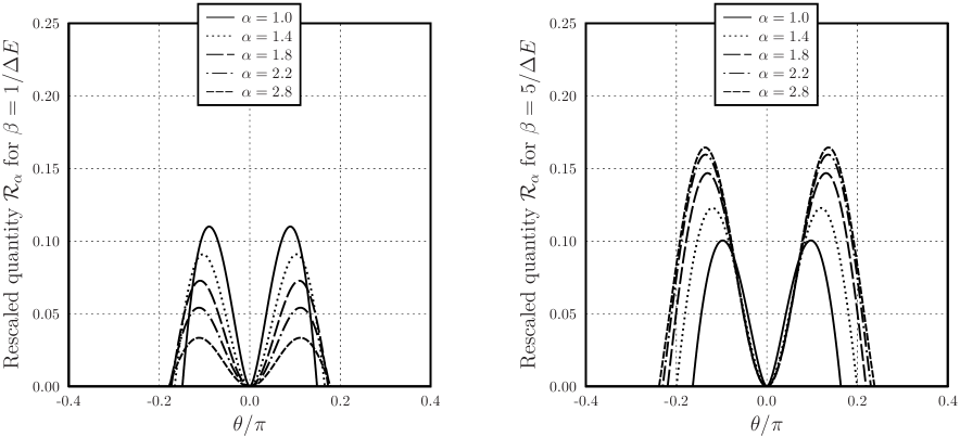
Figure 2: The rescaled characteristic quantity (30) versus $\theta/\pi$ for the qutrit case and several values of $\alpha$, with $\beta=1/\Delta{E}$ on the left plot and $\beta=5/\Delta{E}$ on the right one.

In reality, measurement devices are inevitably exposed to losses. In particular, the detectors used are not perfect, so that the no-click event will sometimes occur. Using the Shannon entropies, the writers of rchtf12 considered the Bell inequalities in the case of detection inefficiencies. For restrictions in terms of generalized entropies, this question was examined in rastqic14 ; rastctp14 . It turned out that the $\alpha$-entropic approach allows us to reduce an amount of required efficiency of detectors. The idealized characteristic quantity ${\mathcal{C}}_{\alpha}$ is given by (29). The macrorealism in the broad sense implies that ${\mathcal{C}}_{\alpha}\leq 0$ for $\alpha\geq 1$. In the case of non-perfect detectors, we will actually deal with the quantity (32). As was noted above, we must confide that the violating term $\eta^{2\alpha}{\mathcal{C}}_{\alpha}$ is considerably large in comparison with the reducing term (33). It is natural to inspect their ratio

$$r_{\alpha}(\eta):=\frac{\Delta_{\alpha}(\eta)}{\eta^{2\alpha}{\mathcal{C}}_{\alpha}}\ ,$$ (38)

which is restricted to the domain, where ${\mathcal{C}}_{\alpha}>0$. Let us consider this ratio in the qubit case with $\beta=5/\Delta{E}$. Here, we set $\theta/\pi=0.15$, so that the strength of violations is large for several values of $\alpha$ (see Fig. 1 on the right). In Fig. 3, we present $r_{\alpha}(\eta)$ versus $\alpha\geq 1$ for several values of $\eta$ close to $1$. For the taken values of the parameters, a robust detection of violations is hardly possible for $\eta<0.95$. If we restrict our consideration to the standard entropies solely, then very high efficiency is required. Using the $\alpha$-entropic approach allows us to minimize (38). As is seen in Fig. 3, this ratio essentially decreases with growth of $\alpha>1$. For $\alpha\in(2;3)$, we are able to reach more reliable detection of violations with the same measurement statistics. For other choices of the parameters, a general picture is similar. In any case, there are physical situations, in which variations of the entropic parameter give additional possibilities to analyze data about work fluctuations. In this sense, the $\alpha$-entropic approach to quantum work fluctuations also deserves to be used in studies of thermodynamics of small systems.

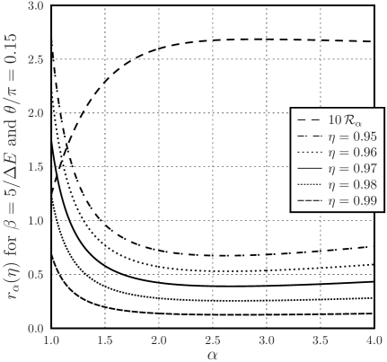
Figure 3: The ratio (38) versus $\alpha$ for the qubit case with $\beta=5/\Delta{E}$, $\theta/\pi=0.15$ and several values of $\eta$. For convenience of referencing to Fig. 1, one also shows values of $\mathcal{R}_{\alpha}$ multiplied by ten.

V Conclusions

We have studied quantum work fluctuations on the base of $\alpha$-entropic Leggett–Garg inequalities. For all $\alpha\geq 1$, such inequalities express restrictions imposed by the macrorealism on outcomes of measurements at different moments of time. It turned out that microscopic ways to realize the quantum work sometimes show statistical correlations inconsistent with the macrorealism in the broad sense. Using the non-extensive entropies allows us to reach additional possibilities in detecting violations of Leggett–Garg inequalities. There are physically motivated situations, in which the $\alpha$-entropic approach leads to an extension of the domain of visible violations. Our findings were illustrated with examples of a single qubit and a single qutrit. As was mentioned in bm17 , for a qubit the Leggett–Garg inequalities in terms of the Shannon entropies are violated independently of the initial temperature. In opposite, the $\alpha$-entropic approach to quantum work fluctuations versus the macrorealism is sensitive to the temperature. Another reason to use the $\alpha$-entropies concerns the case of detection inefficiencies. This case can naturally be considered within the entropic approach. Varying $\alpha>1$, we are sometimes able to reduce essentially an amount of required efficiency of detectors. Dealing with quantum work fluctuations, information-theoretic functions of the Tsallis type should certainly be kept in mind. Induced measures may give additional possibilities to examine data, even though from time to time only.

References

- (1) C. Jarzynski, Annu. Rev. Condens. Matter Phys. 2 (2011) 329–351.
- (2) M. Horodecki, J. Oppenheim, Nat. Commun. 4 (2013) 2059.
- (3) V. Narasimhachar, G. Gour, Nat. Commun. 6 (2015) 7689.
- (4) F. Brandão, M. Horodecki, N. Ng, J. Oppenheim, S. Wehner, Proc. Natl. Acad. Sci. U.S.A. 112 (2015) 3275–3279.
- (5) P. Ćwikliński, M. Studziński, M. Horodecki, J. Oppenheim, Phys. Rev. Lett. 115 (2015) 210403.
- (6) M. Lostaglio, K. Korzekwa, D. Jennings, T. Rudolph, Phys. Rev. X 5 (2015) 021001.
- (7) Á.M. Alhambra, L. Masanes, J. Oppenheim, C. Perry, Phys. Rev. X 6 (2016) 041017.
- (8) S. Vinjanampathy, K. Modi, Int. J. Quantum Inf. 14 (2016) 1640033.
- (9) J. Goold, M. Huber, A. Riera, L. del Rio, P. Skrzypczyk, J. Phys. A: Math. Theor. 49 (2016) 143001.
- (10) T. Albash, D.A. Lidar, M. Marvian, P. Zanardi, Phys. Rev. E 88 (2013) 032146.
- (11) A.E. Rastegin, J. Stat. Mech.: Theor. Exp. (2013) P06016.
- (12) A.E. Rastegin, K. Życzkowski, Phys. Rev. E 89 (2014) 012127.
- (13) J. Åberg, Phys. Rev. X 8 (2018) 011019.
- (14) N. Liu, J. Goold, I. Fuentes, V. Vedral, K. Modi, D.E. Bruschi, Class. Quantum Grav. 33 (2016) 035003.
- (15) D. Bohm, Quantum Theory, Prentice-Hall, Englewood Cliffs, 1951.
- (16) A. Einstein, B. Podolsky, N. Rosen, Phys. Rev. 47 (1935) 777–780.
- (17) J.S. Bell, Physics 1 (1964) 195–200.
- (18) A.J. Leggett, A. Garg, Phys. Rev. Lett. 54 (1985) 857–860.
- (19) C. Emary, N. Lambert, F. Nori, Rep. Prog. Phys. 77 (2014) 016001.
- (20) A. Shafiee, M. Golshani, Fortschr. Phys. 53 (2005) 105–113.
- (21) N. Brunner, D. Cavalcanti, S. Pironio, V. Scarani, S. Wehner, Rev. Mod. Phys. 86 (2014) 419–478.
- (22) D. Rosset, J.-D. Bancal, N. Gisin, J. Phys. A: Math. Theor. 47 (2014) 424022.
- (23) J.F. Clauser, M.A. Horne, A. Shimony, R.A. Holt, Phys. Rev. Lett. 23 (1969) 880–884.
- (24) S.L. Braunstein, C.M. Caves, Phys. Rev. Lett. 61 (1988) 662–665.
- (25) A.R. Usha Devi, H.S. Karthik, Sudha, A.K. Rajagopal, Phys. Rev. A 87 (2013) 052103.
- (26) R. Chaves, T. Fritz, Phys. Rev. A 85 (2012) 032113.
- (27) P. Kurzyński, R. Ramanathan, D. Kaszlikowski, Phys. Rev. Lett. 109 (2012) 020404.
- (28) R. Chaves, Phys. Rev. A 87 (2013) 022102.
- (29) A.E. Rastegin, Quantum Inf. Comput. 14 (2014) 0996–1013.
- (30) M. Wajs, P. Kurzyński, D. Kaszlikowski, Phys. Rev. A 91 (2015) 012114.
- (31) A.E. Rastegin, Ann. Phys. 355 (2015) 241–257.
- (32) Z.-A. Jia, Y.-C. Wu, G.-C. Guo, Phys. Rev. A 96 (2017) 032122.
- (33) R. Blattmann, K. Mølmer, Phys. Rev. A 96 (2017) 012115.
- (34) C. Jarzynski, Phys. Rev. Lett. 78 (1997) 2690–2693.
- (35) C. Jarzynski, Phys. Rev. E 56 (1997) 5018–5035.
- (36) G.E. Crooks, J. Stat. Phys. 90 (1998) 1481–1487.
- (37) G.E. Crooks, Phys. Rev. E 60 (1999) 2721–2726.
- (38) M. Campisi, P. Hänggi, P. Talkner, Rev. Mod. Phys. 83 (2011) 771–791.
- (39) P. Solinas, S. Gasparinetti, Phys. Rev. E 92 (2015) 042150.
- (40) P. Solinas, H.J.D. Miller, J. Anders, Phys. Rev. A 96 (2017) 052115.
- (41) P.P. Hofer, A.A. Clerk, Phys. Rev. Lett. 116 (2016) 013603.
- (42) P. Solinas, S. Gasparinetti, Phys. Rev. A 94 (2016) 052103.
- (43) A. Rényi, Proceedings of the 4th Berkeley Symposium on Mathematical Statistics and Probability, University of California Press, Berkeley, CA, 1961, p. 547.
- (44) C. Tsallis, J. Stat. Phys. 52 (1988) 479–487.
- (45) A.E. Rastegin, Commun. Theor. Phys. 62 (2014) 320–326.
- (46) J. Kofler, C̆. Brukner, Phys. Rev. Lett. 101 (2008) 090403.
- (47) J. Kofler, C̆. Brukner, Phys. Rev. A 87 (2012) 052115.
- (48) S. Abe, Physica A 300 (2001) 417–423.
- (49) S. Abe, A.K. Rajagopal, Physica A 340 (2004) 50–56.
- (50) M. Gell-Mann, C. Tsallis, ed., Nonextensive Entropy – Interdisciplinary Applications, Oxford University Press, Oxford, 2004.
- (51) A.E. Rastegin, Graphs Combin. 32 (2016) 2625–2641.
- (52) A.E. Rastegin, J. Phys. A: Math. Theor. 50 (2017) 215204.
- (53) J. Havrda, F. Charvát, Kybernetika 3 (1967) 30–35.
- (54) M.A. Nielsen, I.L. Chuang, Quantum Computation and Quantum Information, Cambridge University Press, Cambridge, 2000.
- (55) G.A. Raggio, J. Math. Phys. 36 (1995) 4785–4791.
- (56) L. Borland, A.R. Plastino, C. Tsallis, J. Math. Phys. 39 (1998) 6490–6501.
- (57) S. Abe, Phys. Rev. E 66 (2002) 046134.
- (58) S. Abe, Physica A 344 (2004) 359–365.
- (59) S. Furuichi, K. Yanagi, K. Kuriyama, J. Math. Phys. 45 (2004) 4868–4877.
- (60) Ambedkar Dukkipati, M. Narasimha Murty, Shalabh Bhatnagar, Physica A 361 (2006) 124–138.
- (61) S. Furuichi, J. Math. Phys. 47 (2006) 023302.
- (62) X. Hu, Z. Ye, J. Math. Phys. 47 (2006) 023502.
- (63) A.E. Rastegin, J. Stat. Phys. 143 (2011) 1120–1135.
- (64) G.M. Bosyk, S. Zozor, F. Holik, M. Portesi, P.W. Lamberti, Quantum Inf. Process. 15 (2016) 3393–3420.
- (65) G.M. Bosyk, G. Bellomo, S. Zozor, M. Portesi, P.W. Lamberti, Physica A 462 (2016) 930–939.
- (66) P. Jizba, T. Arimitsu, Ann. Phys. 312 (2004) 17–59.
- (67) I. Bengtsson, K. Życzkowski, Geometry of Quantum States: An Introduction to Quantum Entanglement, Cambridge University Press, Cambridge, 2006.
- (68) T.M. Cover, J.A. Thomas, Elements of Information Theory, John Wiley & Sons, New York, 1991.
- (69) Z. Daróczy, Inf. Control 16 (1970) 36–51.
- (70) A.E. Rastegin, Kybernetika 48 (2012) 242–253.
- (71) A.E. Rastegin, RAIRO–Theor. Inf. Appl. 49 (2015) 67–92.
- (72) S. Abe, A.K. Rajagopal, Physica A 289 (2001) 157–164.
- (73) E.M. Purcell, R.V. Pound, Phys. Rev. 81 (1951) 279–280.
- (74) N.F. Ramsey, Phys. Rev. 103 (1956) 20–28.
- (75) J. Dunkel, S. Hilbert, Nature Phys. 10 (2014) 67–72.