Abstract

We present a new feasible way to flatten the axial intensity oscillations for diffraction of a finite-sized Bessel beam, through designing a cardioid-like hole. The boundary formula of the cardioid-like hole is given analytically. Numerical results by the complete Rayleigh-Sommerfeld method reveal that the Bessel beam propagates stably in a considerably long axial range, after passing through the cardioid-like hole. Compared with the gradually absorbing apodization technique in previous papers, in this paper a hard truncation of the incident Bessel beam is employed at the cardioid-like hole edges. The proposed hard apodization technique takes two advantages in suppressing the axial intensity oscillations, i.e., easier implementation and higher accuracy. It is expected to have practical applications in laser machining, light sectioning, or optical trapping.

Flattening axial intensity oscillations of a diffracted Bessel beam through a cardioid-like hole

Jia-Sheng Ye,$*$ Li-Juan Xie, Xin-Ke Wang, Sheng-Fei Feng, Wen-Feng Sun, and Yan Zhang

Department of Physics, Capital Normal University,

Beijing Key Laboratory of Metamaterials and Devices,

Beijing Advanced Innovation Center for Imaging Technology,

Key Laboratory of Terahertz Optoelectronics, Ministry of Education, Beijing 100048, P. R. China

^∗Corresponding author: jsye@mail.cnu.edu.cn

OCIS codes: (050.1970) Diffractive optics; (220.1230) Apodization; (070.7345) Wave propagation.

1 Introduction

The nondiffracting beam exhibits a strict propagating invariance property in free space with good axial intensity uniformity as well as stable transverse resolution [1]. Therefore, it attracts intensive research interest due to its wide applications in laser machining [2], light sectioning [3], interferometry [4], optical trapping [5, 6], microscopy [7] and so on. Durnin et al. have demonstrated mathematically that the three-dimensional infinite-sized Bessel beams are exact solutions to the scalar wave equations [8, 9]. However, it is physically impossible to generate an infinite-sized Bessel beam, in that it is not square integrable and contains infinite energy. Approximate Bessel beams were created in experiments by using an annular slit in the back focal plane of a lens [10, 11, 12], holographic techniques [12, 13, 14, 15], axicons [16, 17], or other ways [18]. In many previous papers, it was reported that the Bessel beam diffracted from a finite-sized circular hole presented prominent axial intensity oscillations [19, 20, 21]. A sudden cut-off of the incident field leads to the strong diffraction effect at the hole edges. This problem was generally solved by covering a gradually absorbing mask. Almost complete suppression of axial intensity oscillations was achieved through apodization of the incident Bessel beam with flattened Gaussian or trigonometric apodized functions [20, 22, 23].

Although the gradually absorbing apodization technology presents a flat axial intensity profile theoretically, it faces two problems in practical applications. Firstly, the amplitude modulation is usually realized by using the spatial light modulator (SLM) [24, 25, 26, 27, 28], but the transmittance is difficult to be adjusted exactly the same as the expected value. If each pixel on the SLM brings about a transmittance error, the obtained intensity distribution will deviate much away from the ideal one. Secondly, it would be difficult that both the total size and spatial resolution of the SLM meet requirements simultaneously so that the apodized field drops very smoothly around the aperture edges. Based on these two considerations, a question is raised. Can we flatten the axial intensity oscillation of a finite-sized Bessel beam by a hard apodization (HA) technique? Here the HA technique means that there only exists a transmitted hole on the input plane, with other parts being opaque. Gray-level transmittance is no longer used for relieving the experimental difficulty and heightening the achieved intensity accuracy. For comparison, we refer to the gradually absorbing apodization technology as the soft apodization (SA) technique.

This paper is organized as follows. In Section 2, the design principles are described in detail, and the boundary formula of the transmitted hole is deduced analytically. For demonstrating the validity of our proposed strategy, in Section 3 the parameters are given and wave propagating behaviors are simulated by the complete Rayleigh-Sommerfeld method [29]. Physical explanations are also delivered. Section 3 consists of two subsections. In subsection 3.1, axial intensity distributions are calculated, and the intensity uniformity is characterized. In subsection 3.2, intensities on several cross-sectional planes within the beam propagation range are evaluated. A brief conclusion is drawn in Section 4 with some discussions.

2 Boundary formula of the transmitted hole for hard apodization

Let’s first consider the diffraction of a Bessel beam from a finite-sized circular hole. The input plane is the $xy$ plane, which situates at $z_{0}=0$ m. The incident Bessel beam propagates along the $z$-axis, whose amplitude distribution satisfies the $J_{0}(\beta r)$ function, where $J_{0}$ is the zeroth order Bessel function; $\beta$ is the propagation constant; $r=\sqrt{x^{2}+y^{2}}$ denotes the radial distance from an arbitrary source point $(x,y)$ to the origin on the input plane.

In the transmitted region ($z>0$), the field at any point $(x^{\prime},y^{\prime},z)$ is calculated by the complete Rayleigh-Sommerfeld method as [29]

$$E(x^{\prime},y^{\prime},z)=\frac{kz}{i2\pi}\int\int_{\Omega}E_{0}(x,y,0)\frac{\exp(ik\rho)}{\rho^{2}}(1-\frac{1}{ik\rho})\mathrm{d}x\mathrm{d}y\,,$$ (1)

where $k=2\pi/\lambda$ represents the wave vector and $\lambda$ represents the incident wavelength; $\Omega$ denotes integral region of the circular hole; $\rho=\sqrt{(x^{\prime}-x)^{2}+(y^{\prime}-y)^{2}+z^{2}}$ is the distance from the source point $(x,y,0)$ on the input plane to the observation point $(x^{\prime},y^{\prime},z)$. $E_{0}(x,y,0)=J_{0}(\beta r)=J_{0}(\beta\sqrt{x^{2}+y^{2}})$ stands for the incident field. The intensity at the observation point is given by $I(x^{\prime},y^{\prime},z)=|E(x^{\prime},y^{\prime},z)|^{2}$, where $|E|$ represents magnitude of the complex number $E$. On assuming $x^{\prime}=y^{\prime}=0$, we will obtain the axial intensity distribution of the Bessel beam diffracted from the circular hole. In this case, the axial field can be simplified in polar coordinates as follows:

$$E(0,0,z)=(-ikz)\int_{0}^{R}E_{0}(r,0)\frac{\exp(ik\sqrt{r^{2}+z^{2}})}{r^{2}+z^{2}}[1-\frac{1}{ik\sqrt{r^{2}+z^{2}}}]r\mathrm{d}r\,,$$ (2)

where $R$ is the radius of the circular hole; $E_{0}(r,0)=J_{0}(\beta r)$ represents the incident Bessel beam on the input plane z=0; $r=\sqrt{x^{2}+y^{2}}$ denotes the radial distance on the input plane.

It is well known that strong axial intensity oscillations are encountered due to a hard truncation of the incident field. For suppressing the axial intensity oscillations, in Ref. [20] Cox et al. introduced a trigonometric apodized function as follows

$$T(r)=\begin{cases}1,&r<\epsilon R,\cr\displaystyle{\frac{1+\cos[\pi(r-\epsilon R)/(R-\epsilon R)]}{2}},&\epsilon R\leq r\leq R,\cr 0,&r>R,\end{cases}$$ (3)

where $T(r)$ represents the amplitude transmittance function on the input plane; $\epsilon$ is a smoothing parameter ranging from 0 to 1. Under this SA condition, the transmittance gradually decreases from 1 to 0 within an annular region $r\in[\epsilon R,R]$, as displayed in Fig. 1(a). The green and pink dashed curves depict two circles with radii of $\epsilon R$ and $R$, respectively. It is seen from Fig. 1(a) that the color gradually becomes from red to blue when the radius increases from $\epsilon R$ to $R$. Correspondingly, the transmittance monotonically decreases from 1 to 0. For calculating the transmitted axial intensity, Eq. (2) is used where the input field now becomes $E_{0}(r,0)=J_{0}(\beta r)T(r)$. By using this SA technique, they achieved a flat axial intensity distribution of the diffracted Bessel beam, as seen in Figs. 4(a) and 4(b) in Ref. [20].

Fig. 1: (a) The transmittance distribution on the input plane $z_{0}=0$ m under the soft apodization (SA) condition. The green and pink dashed curves depict two circles with radii of $\epsilon R$ and $R$, respectively. (b) The shadowed annular district represents the equivalent transmitted region at a definite radius $r$, which occupies 2$|\varphi|$ in the angle direction. (c) The transmittance distribution on the input plane under the hard apodization (HA) condition. The cyan solid curve encloses a cardioid-like hole, with transmittance being 1 and 0 inside and outside the hole, respectively.

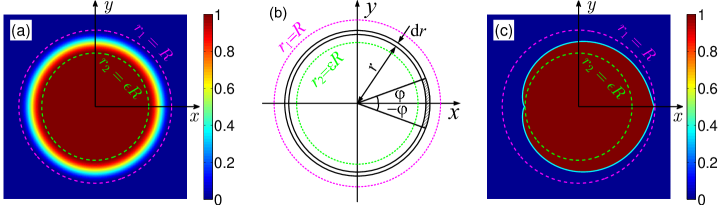
In the following, we will discuss our strategy. From Eq. (2), the field at any axial point $(0,0,z)$ is a diffraction superposition of all the source points on the input plane. Since there is only one integral variable $r$ in Eq. (2), the optical system is rotationally symmetric. Namely, in the input plane each source point on a definite circle with the same radius $r$ has the same incident field $E_{0}(r,0)=J_{0}(\beta r)$, contributing equally to a given axial observation point. Therefore, we can make such a equivalent change. For instance, in Fig. 1(a), if the transmittance $T(r_{0})$ equals 0.5 for some radius $r_{0}$, we may let the incident field passes one half while the other half is blocked at radius $r_{0}$. It is easy to understand that we should get the same axial intensity distributions in both cases. For other transmittance values, the only difference lies in the filling ratio of the transmitted part.

Now we turn to explore the general shape that the transmitted hole should be like. In Fig. 1(b), the shadowed region represents the equivalent transmitted part for a given radius $r$ within $r\in[\epsilon R,R]$. The filling ratio $F(r)$ should fulfill the following equation

$${F(r)=\frac{2|\varphi|}{2\pi}}=T(r)=\displaystyle{\frac{1+\cos[\pi(r-\epsilon R)/(R-\epsilon R)]}{2}},\hskip 28.45274pt-\pi\leq\varphi\leq\pi.$$ (4)

After mathematical transformation, we may write Eq. (4) explicitly as follows

$$r(\varphi)=\epsilon R+\displaystyle{\frac{(R-\epsilon R)\arccos(2|\varphi|/\pi-1)}{\pi}},\hskip 28.45274pt-\pi\leq\varphi\leq\pi.$$ (5)

All the points satisfying Eq. (5) form a closed curve, as drawn by the cardioid-like cyan solid curve in Fig. 1(c). From the above analysis, if the incident Bessel beam passes through a cardioid-like hole while it is prevented outside, we can expect the same flat axial intensity distribution as that in Ref. [20]. Figure 1(c) shows the transmittance distribution on the input plane under the proposed HA condition, indicating the transmittance being 1 and 0 inside and outside the region encircled by the cardioid-like curve, respectively.

3 Propagating behaviors of the apodized Bessel beams

In this section, we will perform numerical simulations to prove the validity of the proposed HA technique. Parameters are chosen as follows. For the incident Bessel beam, the propagation constant is $\beta=10^{4}~{}\mathrm{m}^{-1}$ with wavelength of $\lambda=0.5~{}\mu\mathrm{m}$. The circular hole has a radius of $R=50~{}\mathrm{mm}$.

3.1 The axial intensity distribution of the apodized Bessel beam

Fig. 2: (a) The axial intensity distribution of the Bessel beam diffracted from a circular hole without apodization. (b) The blue solid and red dashed curves represent the axial intensity distributions of the diffracted Bessel beam by the SA and HA techniques, corresponding to Figs. 1(a) and 1(c), respectively. In both cases, we choose the same smoothing parameter as $\epsilon_{0}=0.5$. (c) Axial intensity distributions of the diffracted Bessel beam by the HA technique, when the smoothing parameter $\epsilon$ varies from 0.7 to 0.9 with an interval of 0.05. The blue, green, red, cyan, and black curves correspond to different smoothing parameters of 0.7, 0.75, 0.8, 0.85, and 0.9, respectively.

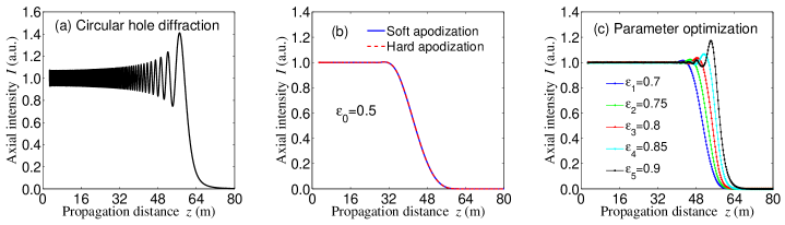
In this subsection, the axial intensity distribution of the diffracted Bessel beam is investigated. Firstly, by assuming $E_{0}(r,0)$ to be $J_{0}(\beta r)$ in Eq. (2), we can obtain the axial intensity distribution of the diffracted Bessel beam from a finite-sized circular hole without apodization, as shown by the black curve in Fig. 2(a). It is seen from Fig. 2(a) that the axial intensity oscillates with a relative error of about $\pm 7\%$. Secondly, axial intensity profiles are flattened by the SA and HA techniques to prove their equivalence, as shown by the blue solid and red dashed curves in Fig. 2(b), respectively. In both cases, we choose the same smoothing parameter $\epsilon_{0}$ as 0.5. Under the SA condition, the incident field on the input plane in Eq. (2) is given by $E_{0}^{\mathrm{s}}(r,0)=J_{0}(\beta r)\times T(r)$, where $T(r)$ is given by Eq. (3). The integral region $\Omega_{1}$ is the circular hole. Under the HA condition, since the cardioid-like hole is rotationally asymmetric, axial intensity should be calculated from Eq. (1), where the incident field on the input plane is $E_{0}(x,y,0)=J_{0}(\beta\sqrt{x^{2}+y^{2}})$ and the integral region $\Omega_{2}$ is the cardioid-like hole determined by Eq. (5). It is demonstrated in Fig. 2(b) that both curves overlap, namely, we have achieved the same flat axial intensity distributions of the diffracted Bessel beam by the previous SA and the proposed HA techniques. Thirdly, through optimizing the smoothing parameter $\epsilon$ in Eq. (5), we have computed the diffracted axial intensity distributions of the Bessel beam enclosed by the cardioid-like curve, as drawn in Fig. 2(c). The smoothing parameter $\epsilon$ ranges from 0.7 to 0.9 for every 0.05. The blue, green, red, cyan, and black curves correspond to different smoothing parameters of 0.7, 0.75, 0.8 ,0.85, and 0.9, respectively. With the increase of the smoothing parameter, the propagation distance is lengthened while the axial intensity uniformity is weakened, as observed in Fig. 2(c). It can be interpreted. When the smoothing parameter becomes larger, the transmittance drops more rapidly from 1 to 0 near the hole edges. Therefore, the diffraction effect is stronger and the axial intensity oscillations appear to be more prominent. When the smoothing parameter $\epsilon$ reaches 1, it degenerates to the case in Fig. 2(a). On taking both the axial intensity uniformity and the propagation distance into account, the smoothing parameter is compromised as 0.8 in the following.

Next, the axial intensity uniformity is quantitatively characterized when the smoothing parameter is 0.8. The flat axial intensity region is defined as the axial domain with intensity relative error less than $\pm 0.01\%$. Numerical results reveal that the flat axial intensity region extends out to $z_{f}=32.01$ m. The axial range expands to 39.15 and 46.42 m when the restriction of intensity relative error is relaxed to $\pm 0.1\%$ and $\pm 1\%$, respectively. Then, the axial intensity oscillations are gradually strengthened. After the axial intensity reaches its peak value of 1.037 at $z_{f}=48.44$m, it drops rapidly towards 0. When the propagation distance is longer than 61.46 m, the axial intensity drops below 1%. The numerical simulations agree well with the results obtained from geometrical optics. Since the Bessel beam can be considered as superposition of plane waves whose wave vectors lie on a cone with an angle $\theta$ with respect to the $z$-axis [10, 20], where $\beta=k\sin(\theta)=2\pi\sin(\theta)/\lambda$. In geometrical optics, the effective axial beam range is given by $z_{\mathrm{max}}=R/\tan(\theta)=62.83$ m.

3.2 Intensity distributions on several cross-sectional planes for the hard apodized Bessel beam

Fig. 3: Intensity deviation on three cross-sectional planes for the hard apodized Bessel beam. The smoothing parameter $\epsilon$ is 0.8, and other parameters are the same as above. (a) The intensity deviation $\Delta I_{1}=I_{1}(x_{1},y_{1})-I_{0}(x,y)$, where $I_{1}(x_{1},y_{1})$ represents the intensity distribution on the lateral plane $z_{1}=10$ m and $I_{0}(x,y)=|J_{0}(\beta\sqrt{x^{2}+y^{2}})|^{2}$ is the intensity of the incident Bessel beam on the input plane $z_{0}=0$ m. (b) and (c) are the same as (a) except for $z_{2}=20$ m and $z_{3}$=30 m, respectively.

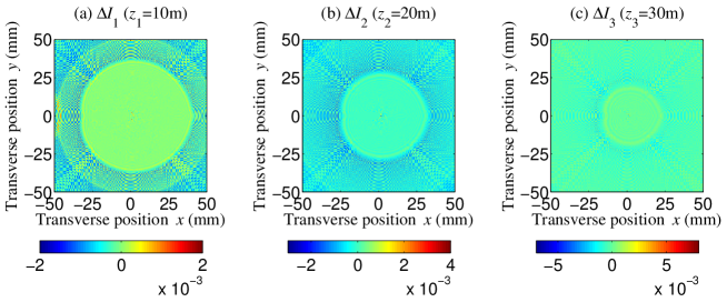
Since the cardioid-like curve in Fig. 1(c) is rotationally asymmetric, the field on cross-sectional planes should also be asymmetric. In this case, the transmitted intensity distributions are calculated from Eq. (1) and the integral region $\Omega$ is the cardioid-like hole. To see how asymmetric the field is, figure 3 displays the regional intensity deviation on three cross-sectional planes. Figure 3(a) presents the intensity deviation $\Delta I_{1}=I_{1}(x_{1},y_{1})-I_{0}(x,y)$, where $I_{1}(x_{1},y_{1})$ represents the intensity distribution on the lateral plane $z_{1}=10$ m and $I_{0}(x,y)=|J_{0}(\beta\sqrt{x^{2}+y^{2}})|^{2}$ is the intensity of the incident Bessel beam on the input plane $z_{0}=0$ m. Figures 3(b) and 3(c) are the same as Fig. 3(a) except for $z_{2}=20$ m, and $z_{3}=30$ m, respectively. A cardioid-like shape of intensity deviation is observed in Fig. 3, which suggests that asymmetry of the cardioid-like hole leads to the intensity asymmetry. With the propagation of Bessel beam, the size of the cardioid-like shape is gradually decreased. The intensity deviation is in the magnitude of $10^{-3}$ from the color bars, indicating the intensity relative error is less than 1%. Accordingly, the diffracted Bessel beam preserves a relatively stable propagation property in a considerably long axial range, although somewhat asymmetric.

Fig. 4: The intensity distributions on three cross-sectional planes with longitudinal coordinates of (a) $z_{1}$=10 m, (b) $z_{2}$=20 m, and (c) $z_{3}$=30 m, respectively. The smoothing parameter $\epsilon$ is assumed to be 0.8, and other parameters are the same as above. The blue solid and red dashed curves represent the intensity profiles along the $x$-axis and the $y$-axis, respectively. (d) Intensity deviation $\Delta I_{x}=I_{i}(x_{i},0)-|J_{0}(\beta|x|)|^{2}$ and $\Delta I_{y}=I_{i}(0,y_{i})-|J_{0}(\beta|y|)|^{2}$ on the above-mentioned three cross-sectional planes are displayed from top to bottom, where $I_{i}(x_{i},0)$ and $I_{i}(0,y_{i})$ (i=1,2,3) represent the intensities along the $x$-axis and the $y$-axis, respectively.

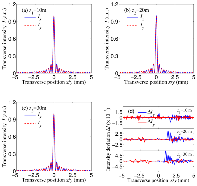
To see the intensity asymmetry property more clearly, we extract the intensity distributions along the $x$-axis and the $y$-axis on the above three cross-sectional planes, as shown in Figs. 4(a), 4(b), and 4(c). The blue solid and red dashed curves correspond to intensities along the $x$-axis and the $y$-axis, respectively. It is seen from Figs. 4(a) to 4(c) that the intensity profiles on both axes almost overlap. In order to magnify the intensity difference along the $x$-axis and the $y$-axis, we calculate the intensity deviation $\Delta I_{x}=I_{i}(x_{i},0)-|J_{0}(\beta|x|)|^{2}$ and $\Delta I_{y}=I_{i}(0,y_{i})-|J_{0}(\beta|y|)|^{2}$ on the three cross-sectional planes, as shown by the blue and red curves in Fig. 4(d) from top to bottom. $I_{i}(x_{i},0)$ and $I_{i}(0,y_{i})$ (i=1,2,3) represent the intensities along the $x$-axis and the $y$-axis, respectively. The intensity deviation $\Delta I_{x}$ or $\Delta I_{y}$ presents the difference between the intensity at the observation point and that at the corresponding point on the input plane, indicating the propagation invariance property. It is seen from Fig. 4(d) that the red curves ($\Delta I_{y}$) are symmetric about the origin point while the blue curves ($\Delta I_{x}$) are asymmetric about the origin point. The reason is that the cardioid-like hole is symmetric about the $x$-axis but asymmetric about the $y$-axis. Since the maximum intensity deviation is less than $\pm 10^{-2}$, the diffracted Bessel beam propagates relatively stably within the beam propagation range. If we calculate the asymmetric intensity difference $\Delta I_{xy}=I_{x}-I_{y}=\Delta I_{x}-\Delta I_{y}$, the intensity asymmetric property will be quantified. The intensity asymmetry does exist since the two curves in Fig. 4(d) are clearly separated. However, the maximum asymmetric intensity difference $\Delta I_{xy}$ is only 0.89%. Especially, for applications of Bessel beams we are generally interested in a few lobes near the center. The asymmetric intensity difference $\Delta I_{xy}$ is below 0.12% for the central five intensity lobes. Consequently, the intensity asymmetry can almost be neglected in the paraxial region.

4 Conclusion and discussions

In this paper, we present a new feasible way to flatten the diffracted axial intensity distribution of a finite-sized Bessel beam. Numerical results by the complete Rayleigh-Sommerfeld method have validated our strategy. It is found that the Bessel beam diffracted from a cardioid-like hole maintains a very good propagating invariance property along the axial direction. The boundary formula of the cardioid-like hole is given analytically. Compared with the previous SA technique, the proposed HA technique provides a more feasible choice in practical applications with higher accuracy, since the error only comes from the hole boundary.

In fact, the proposed HA technique is a universal method for suppressing the axial intensity oscillations, by transforming the transmittance distribution into spatial transmitted filling factors. Therefore, for other amplitude transmittance functions like the flattened Gaussian shape, by analogy we can obtain another closed transmitted hole on the input plane. Moreover, the proposed method may be extended to suppress axial intensity oscillations for other kinds of incident waves, such as plane waves or Gaussian waves. It is expected to have practical applications in many optical processing systems.