A Monotone Finite Volume Method for Time Fractional Fokker-Planck Equations

Abstract

We develop a monotone finite volume method for the time fractional Fokker-Planck equations and theoretically prove its unconditional stability. We show that the convergence rate of this method is order 1 in space and if the space grid becomes sufficiently fine, the convergence rate can be improved to order 2. Numerical results are given to support our theoretical findings. One characteristic of our method is that it has monotone property such that it keeps the nonnegativity of some physical variables such as density, concentration, etc.

2000 Mathematics subject classification: 65M12, 65M06, 35S10

Keywords: time fractional Fokker-Planck equations, finite volume methods

1 Introduction

This paper considers the time fractional Fokker-Planck equation (FFPE)

$$\frac{\partial w}{\partial t}=\,_{0}D^{1-\alpha}_{t}\left[k_{\alpha}\frac{\partial^{2}}{\partial x^{2}}-\frac{\partial}{\partial x}f(x)\right]w(x,t),\quad a\leq x\leq b,0<t\leq T,$$ (1.1)

subject to the initial condition

$$w(x,0)=\varphi(x),\quad a\leq x\leq b,$$ (1.2)

and boundary conditions

$$w(a,t)=g_{1}(t),\quad w(b,t)=g_{2}(t),\quad 0<t\leq T,$$ (1.3)

where $\alpha\in(0,1)$, $k_{\alpha}$ is a positive constant, $f(x),\phi(x),g_{1}(t),g_{2}(t)$ are given functions, and $\,{}_{0}D^{1-\alpha}_{t}w(x,t)=\frac{1}{\Gamma(\alpha)}\frac{\partial}{\partial t}\int_{0}^{t}\frac{w(x,s)}{(t-s)^{1-\alpha}}ds$ is the Riemann-Liouville fractional derivative of order $1-\alpha$ with $\Gamma(x)$ being the gamma function.

When the equation (1.1) is used to model the sub-diffusion processes in an external force field (see e.g. [23, 24, 30, 31]), $k_{\alpha}$ denotes the generalized diffusion coefficient, and $f(x)=\frac{v^{\prime}(x)}{m\eta_{\alpha}}$ represents the external force field governed by the potential $v^{\prime}(x)$ with $m$ being the mass of the diffusion particle and $\eta_{\alpha}$ the generalized friction coefficient.

Under the condition that problem {(1.1)-(1.3)} admits a unique solution $w(x,t)\in C^{2,1}_{x,t}[a,b]\times[0,T]$, the equation (1.1) may be rewritten in the following equivalent form (see e.g. [3]):

$$\frac{\partial^{\alpha}w}{\partial t^{\alpha}}=\left[k_{\alpha}\frac{\partial^{2}}{\partial x^{2}}-\frac{\partial}{\partial x}f(x)\right]w(x,t),\quad a\leq x\leq b,0<t\leq T,$$ (1.4)

where ${\partial^{\alpha}w}/{\partial t^{\alpha}}$ denotes the Caputo fractional derivative of order $\alpha(0<\alpha<1)$ defined by

$$\frac{\partial^{\alpha}w(x,t)}{\partial t^{\alpha}}=\frac{1}{\Gamma(1-\alpha)}\int_{0}^{t}\frac{\partial w(x,\eta)}{\partial t}\frac{d\eta}{(t-\eta)^{\alpha}}.$$

For the time FFPE, lots of numerical works have been done and most of them concern the case $f(x)=0$ (see e.g., [15, 16, 18, 19, 20, 22, 25, 35, 36]). Some works on the numerical solution of (1.4) with $f(x)\neq 0$ are listed as follows: Saadatmandi et al. [28] study a collocation method based on shifted Legendre polynomials in time and Sinc functions in space; Fairweather et al. [7], using the $L_{1}$ approximation to the time fractional derivative, investigate an orthogonal spline collocation method in space; Deng [5] and Cao et al. [2] study numerical schemes for ODE systems derived from spatial semi discretization of (1.4).

To numerically solve (1.4), Chen et al. [3] present three implicit finite difference schemes and obtain the stability and convergence under conditions that $f(x)$ is a constant or a monotone function. Jiang [13] establishes monotone properties of the numerical schemes given in [3], based on which, a new proof of stability and convergence is provided under a weaker condition $f(x)\in C[a,b]$. Recently, Vong and Wang [33] develop a high order compact difference scheme for (1.4), and obtain its stability and convergence. In both [13] and [33], the stability and convergence are derived under the condition $h|f(x)|\leq C$ ($h$ denotes space step size and $C$ is a constant), which requires sufficiently fine space grid in order to obtain desirable numerical solutions when $|f(x)|$ is large.

Finite volume (FV) methods, after being successfully applied to solving integer partial differential equations (see e.g. [32]), have been concerned for solving fractional equations in some literatures: for example, [8, 10, 21, 34] study FV methods for space fractional equations; [9] studies FV methods for time-space fractional equations; [16] investigates a FV element method for a two dimensional time FPDE (the two dimensional case of (1.4) with $f=0$).

We develop a FV method for solving (1.4), using center and upwind differences for space discretization and $L_{1}$ approximation to the time fractional derivative. Under a discrete $L^{1}$-norm, we theoretically prove that our method is unconditionally stable and its convergence order is $O(h+\Delta t^{2-\alpha})$ (the convergence order can be improved to $O(h^{2}+\Delta t^{2-\alpha})$ if the space grid becomes sufficiently fine). Numerical results are given to support our theoretical findings. One characteristic of our method is that it has monotone property such that it keeps the nonnegativity of some physical variables such as density, concentration, etc. and is efficient even on coarse grids for the case that $|f(x)|$ is large.

In this paper, $C$ denotes a generic positive constant independent of grid sizes, which may take on different values at different places. For easy statement, we assume that the solution $w$ is sufficiently smooth and $f(x)$ satisfies the following Lipschitz condition

$$|f(x)-f(x^{\prime})|\leq C|x-x^{\prime}|,\quad x,x^{\prime}\in[a,b].$$ (1.5)

The rest of this paper is organized as follows: in section 2, we introduce a finite volume scheme for solving (1.4); in section 3, we show its monotone property, based on which we prove the stability and convergence of the scheme; in section 4, we carry out some numerical tests to support our theory.

2 Discretisation

For a positive integer $N$, define the space step size $h=(b-a)/(N+1)$ and uniformly-spaced nodes $x_{i}=a+ih,i=0,1,\ldots,N+1$. Then we have $N$ control volumes $[x_{i-\frac{1}{2}},x_{i+\frac{1}{2}}]$, $i=1,2,\ldots,N$. For a positive integer $L$, define $\Delta t=T/L$. We use the uniform time grid $t_{k}=k\Delta t(k=0,1,\ldots,L)$ for discretization of the time fractional derivative.

For simplicity, we use the following conventions: for function $g(x,t)$, $g_{i+\frac{1}{2},n}=(g)_{(x_{i+\frac{1}{2}},t_{n})}:=g(x_{i+\frac{1}{2}},t_{n})$; for function $g(x)$, $g_{i+\frac{1}{2}}=(g)_{x_{i+\frac{1}{2}}}:=g(x_{i+\frac{1}{2}})$. Decompose the function $f(x)$ as

$$f=f^{u}+f^{l}+f^{m},$$

with $f^{u}(x):=\max(f(x)-\frac{2k_{\alpha}}{h},0)$, $f^{l}(x):=\min(f(x)+\frac{2k_{\alpha}}{h},0)$, and $f^{m}:=f-f^{u}-f^{l}$ for $x\in[a,b]$. It is not hard to see that $f^{u},f^{l},$ and $f^{m}$ each satisfy the Lipschitz condition with the same positive $C$ as that in (1.5) and

$$f^{u}(x)\geq 0,\quad f^{l}(x)\leq 0,\quad-\frac{2k_{\alpha}}{h}\leq f^{m}(x)\leq\frac{2k_{\alpha}}{h}.$$ (2.1)

Remark 2.1

In designing the numerical method that follows, we only use the values of functions $f^{m}$, $f^{u}$ and $f^{l}$ at points $x_{i+\frac{1}{2}}$ ($i=0,1,\ldots,N$), i.e., $f^{m}_{i+\frac{1}{2}}=f^{m}(x_{i+\frac{1}{2}}),f^{u}_{i+\frac{1}{2}}=f^{u}(x_{i+\frac{1}{2}}),f^{l}_{i+\frac{1}{2}}=f^{l}(x_{i+\frac{1}{2}})$.

Evaluating (1.4) at $t=t_{n}$ $(n=1,2,\ldots,L)$ and integrating equation (1.4) over the $i$th control volume $[x_{i-\frac{1}{2}},x_{i+\frac{1}{2}}]$ give

$$\int_{x_{i-\frac{1}{2}}}^{x_{i+\frac{1}{2}}}\left.\frac{\partial^{\alpha}w}{\partial t^{\alpha}}\right|_{t_{n}}dx = k_{\alpha}\left(\left(\frac{\partial w}{\partial x}\right)_{{i+\frac{1}{2}},n}-\left(\frac{\partial w}{\partial x}\right)_{{i-\frac{1}{2}},n}\right)$$ (2.2)

$$\quad-\quad\left((fw)_{{i+\frac{1}{2}},n}-(fw)_{i-\frac{1}{2},n}\right),$$

$i=1,2,\ldots,N$. Denote $w(x_{i},t_{n})$ by $w_{i}^{n}$ ($i=0,\ldots,N+1,n=0,1,\ldots,L$). The left hand term of (2.2) may be written as

$$\int_{x_{i-\frac{1}{2}}}^{x_{i+\frac{1}{2}}}\left.\frac{\partial^{\alpha}w}{\partial t^{\alpha}}\right|_{t_{n}}dx=\left(\frac{\partial^{\alpha}w}{\partial t^{\alpha}}\right)_{(x_{i},t_{n})}h-h\gamma^{(1)}_{i,n}$$ (2.3)

$$= \frac{h\Delta t^{-\alpha}}{\Gamma(2-\alpha)}\left(w_{i}^{n}-\sum\limits_{k=1}^{n-1}(a_{n-k-1}-a_{n-k})w_{i}^{k}-a_{n-1}w_{i}^{0}\right)-h\gamma^{(1)}_{i,n}-h\gamma^{(2)}_{i,n},$$

where the mid rectangular integral formula is used in the first equality, the $L_{1}$ approximation is used in the second equality with $a_{k}=(k+1)^{1-\alpha}-k^{1-\alpha}$ ($k=0,1,2,\ldots$)(see [26, 17]), and the truncation errors

$$\gamma^{(1)}_{i,n}:=\left(\left(\frac{\partial^{\alpha}w}{\partial t^{\alpha}}\right)_{(x_{i},t_{n})}h-\int_{x_{i-\frac{1}{2}}}^{x_{i+\frac{1}{2}}}\left.\frac{\partial^{\alpha}w}{\partial t^{\alpha}}\right|_{t_{n}}dx\right)/h,$$

$$\gamma^{(2)}_{i,n}:=\left(\frac{h\Delta t^{-\alpha}}{\Gamma(2-\alpha)}\left(w_{i}^{n}-\sum\limits_{k=1}^{n-1}(a_{n-k-1}-a_{n-k})w_{i}^{k}-a_{n-1}w_{i}^{0}\right)-h\left(\frac{\partial^{\alpha}w}{\partial t^{\alpha}}\right)_{(x_{i},t_{n})}\right)/h.$$

We have the truncation errors bounds

$$h\left|\gamma^{(1)}_{i,n}\right|\leq Ch^{3},\quad h\left|\gamma^{(2)}_{i,n}\right|\leq Ch\Delta t^{2-\alpha},\quad i=1,\ldots,N;n=1,\ldots,L,$$ (2.4)

where for the second error bound please refer to [17]. The first term on the right hand side of (2.2) can be written as

$$k_{\alpha}\left(\left(\frac{\partial w}{\partial x}\right)_{{i+\frac{1}{2}},n}-\left(\frac{\partial w}{\partial x}\right)_{{i-\frac{1}{2}},n}\right)$$ (2.5)

$$= k_{\alpha}\left(\widehat{\left(\frac{\partial w}{\partial x}\right)}_{{i+\frac{1}{2}},n}-\widehat{\left(\frac{\partial w}{\partial x}\right)}_{{i-\frac{1}{2}},n}\right)+h\gamma^{(3)}_{i,n},$$

where

$$\widehat{\left(\frac{\partial w}{\partial x}\right)}_{{i+\frac{1}{2}},n}:=\frac{w^{n}_{i+1}-w^{n}_{i}}{h},\quad i=0,2,\ldots,N;$$ (2.6)

we have used the midpoint difference formulas for approximations of the derivatives; By Taylor formula, it is easy to see that

$$h\left|\gamma^{(3)}_{i,n}\right|\leq Ch^{3},\quad i=1,2,\ldots,N.$$ (2.7)

The second term on the right hand side of (2.2) is related to the convection speed $f(x)$. We combine the central and upwind differences to rewrite

$$(fw)_{{i+\frac{1}{2}},n}=(f^{m}w)_{{i+\frac{1}{2}},n}+(f^{u}w)_{{i+\frac{1}{2}},n}+(f^{l}w)_{{i+\frac{1}{2}},n}$$ (2.8)

$$= \widetilde{(f^{m}w)}_{i+\frac{1}{2},n}+\widetilde{(f^{u}w)}_{i+\frac{1}{2},n}+\widetilde{(f^{l}w)}_{i+\frac{1}{2},n}+r^{m}_{i+\frac{1}{2},n}+r^{u}_{i+\frac{1}{2},n}+r^{l}_{i+\frac{1}{2},n}$$

for $i=0,1,\ldots,N$, with

$$\widetilde{(f^{m}w)}_{i+\frac{1}{2},n}:=f^{m}_{i+\frac{1}{2}}\frac{w^{n}_{i}+w^{n}_{i+1}}{2},$$ (2.9)

$$\widetilde{(f^{u}w)}_{i+\frac{1}{2},n}:=f^{u}_{i+\frac{1}{2}}w^{n}_{i},\quad\widetilde{(f^{l}w)}_{i+\frac{1}{2},n}:=f^{l}_{i+\frac{1}{2}}w^{n}_{i+1},$$ (2.10)

$$r^{m}_{i+\frac{1}{2},n}:=(f^{m}w)_{i+\frac{1}{2},n}-\widetilde{(f^{m}w)}_{i+\frac{1}{2},n}=-f^{m}_{i+\frac{1}{2}}\left(\frac{\partial^{2}w}{\partial x^{2}}\right)_{i+\frac{1}{2},n}\frac{h^{2}}{8}+O(h^{4}),$$ (2.11)

$$r^{u}_{i+\frac{1}{2},n}:=(f^{u}w)_{i+\frac{1}{2},n}-\widetilde{(f^{u}w)}_{i+\frac{1}{2},n}=f^{u}_{i+\frac{1}{2}}\left(\frac{\partial w}{\partial x}\right)_{i+\frac{1}{2},n}\frac{h}{2}+O(h^{2}),$$ (2.12)

$$r^{l}_{i+\frac{1}{2},n}:=(f^{l}w)_{i+\frac{1}{2},n}-\widetilde{(f^{l}w)}_{i+\frac{1}{2},n}=-f^{l}_{i+\frac{1}{2}}\left(\frac{\partial w}{\partial x}\right)_{i+\frac{1}{2},n}\frac{h}{2}+O(h^{2}).$$ (2.13)

where we have used Taylor formula in (2.11), (2.12) and (2.13). Then the second term on the right hand of (2.2) may be rewritten as

$$(fw)_{{i+\frac{1}{2}},n}-(fw)_{{i-\frac{1}{2}},n}=\widetilde{(fw)}_{i+\frac{1}{2},n}-\widetilde{(fw)}_{i-\frac{1}{2},n}-h\gamma^{(4)}_{i,n},$$ (2.14)

with

$$\widetilde{(fw)}_{i+\frac{1}{2},n}=\widetilde{(f^{m}w)}_{i+\frac{1}{2},n}+\widetilde{(f^{u}w)}_{i+\frac{1}{2},n}+\widetilde{(f^{l}w)}_{i+\frac{1}{2},n}$$ (2.15)

and

$$h\gamma^{(4)}_{i,n}=(r^{m}_{i-\frac{1}{2},n}-r^{m}_{i+\frac{1}{2},n})+(r^{u}_{i-\frac{1}{2},n}-r^{u}_{i+\frac{1}{2},n})+(r^{l}_{i-\frac{1}{2},n}-r^{l}_{i+\frac{1}{2},n}).$$ (2.16)

Remark 2.2

It is easy to deduce that for $i=1,\ldots,N$

$$|r^{m}_{i-\frac{1}{2},n}-r^{m}_{i+\frac{1}{2},n}|\leq Ch^{3},$$

and

$$|r^{u}_{i-\frac{1}{2},n}-r^{u}_{i+\frac{1}{2},n}|\leq Ch^{2},\quad|r^{l}_{i-\frac{1}{2},n}-r^{l}_{i+\frac{1}{2},n}|\leq Ch^{2}.$$

By the definitions of $f^{u}$ and $f^{l}$, $|r^{u}_{i-\frac{1}{2},n}-r^{u}_{i+\frac{1}{2},n}|$ and $|r^{l}_{i-\frac{1}{2},n}-r^{l}_{i+\frac{1}{2},n}|$ become smaller as $h$ becomes smaller, and if ${|f(x)|}\leq\frac{2k_{\alpha}}{h}$, they become zeros since $f^{u}=f^{l}=0$.

Substituting (2.14), (2.5) and (2.3) into (2.2) gives

$$\frac{h\Delta t^{-\alpha}}{\Gamma(2-\alpha)}\left(w_{i}^{n}-\sum\limits_{k=1}^{n-1}(a_{n-k-1}-a_{n-k})w_{i}^{k}-a_{n-1}w_{i}^{0}\right)$$ (2.17)

$$= k_{\alpha}\left(\widehat{\left(\frac{\partial w}{\partial x}\right)}_{{i+\frac{1}{2}},n}-\widehat{\left(\frac{\partial w}{\partial x}\right)}_{{i-\frac{1}{2}},n}\right)-\left(\widetilde{(fw)}_{i+\frac{1}{2},n}-\widetilde{(fw)}_{i-\frac{1}{2},n}\right)+hr^{n}_{i},$$

$i=1,2,\ldots,N$, $n=1,2,\ldots,L$, where $r_{i}^{n}=\sum_{j=1}^{4}\gamma^{(j)}_{i,n}$. We use $W^{n}_{i}$ to denote the approximation of $w^{n}_{i}$. By (2.17), we derive the following finite volume (FV) scheme: for $i=1,2,\ldots,N$, $n=1,2,\ldots,L$,

$$\frac{h\Delta t^{-\alpha}}{\Gamma(2-\alpha)}\left(W_{i}^{n}-\sum\limits_{k=1}^{n-1}(a_{n-k-1}-a_{n-k})W_{i}^{k}-a_{n-1}W_{i}^{0}\right)$$

$$=k_{\alpha}\left(\widehat{\left(\frac{\partial W}{\partial x}\right)}_{{i+\frac{1}{2}},n}-\widehat{\left(\frac{\partial W}{\partial x}\right)}_{{i-\frac{1}{2}},n}\right)-\left(\widetilde{(fW)}_{i+\frac{1}{2},n}-\widetilde{(fW)}_{i-\frac{1}{2},n}\right),$$ (2.18)

subject to boundary values $W^{n}_{0}=g_{1}(t_{n})$, $W^{n}_{N+1}=g_{2}(t_{n})$, $n=1,2,\ldots,L$ and initial values $W^{0}_{i}$ are taken as the approximations to $w^{0}_{i}=\phi(x_{i})$, $i=1,\ldots,N$, where $\widehat{\left(\frac{\partial W}{\partial x}\right)}_{{i+\frac{1}{2}},n}$ are defined by directly replacing $w$ with $W$ in (2.6), $\widetilde{(fW)}_{i+\frac{1}{2},n}$ are defined by directly replacing $w$ with $W$ in (2.15), (2.9) and (2.10).

The matrix form of the FV scheme is

$$\left(\frac{h\Delta t^{-\alpha}}{\Gamma(2-\alpha)}I+A+B\right)W^{n}=\frac{h\Delta t^{-\alpha}}{\Gamma(2-\alpha)}\left(\sum\limits_{k=1}^{n-1}(a_{n-k-1}-a_{n-k})W^{k}+a_{n-1}W^{0}\right)+d^{n},$$ (2.19)

$n=1,2,\ldots,L$, where $W^{k}=(W^{k}_{1},\ldots,W^{k}_{N})^{T}$, $d^{n}=(d^{n}_{1},d^{n}_{2},\ldots,d^{n}_{N})\in R^{N}$, $I\in R^{N\times N}$ is the identity matrix, $A=(a_{ij})\in R^{N\times N}$ is the coefficient matrix corresponding to the first term of the right hand side (2), $B=(b_{ij})\in R^{N\times N}$ is the coefficient matrix corresponding to the second term of the right hand side (2), the entries of $A,B,d^{n}$ are listed as follows:

the $1$th column of $A$

$$a_{11}=\frac{2k_{\alpha}}{h},\quad a_{21}=-\frac{k_{\alpha}}{h},\quad a_{i1}=0,i\geq 3;$$ (2.20)

the $N$th column of $A$

$$a_{NN}=\frac{2k_{\alpha}}{h},\quad a_{(N-1)N}=-\frac{k_{\alpha}}{h},\quad a_{iN}=0,i\leq N-2;$$ (2.21)

the $j$th column of $A$ ($j=2,\ldots,N-1$)

$$a_{jj}=\frac{2k_{\alpha}}{h},\quad a_{(j+1)j}=a_{(j-1)j}=-\frac{k_{\alpha}}{h},\quad a_{ij}=0,i\geq j+2\hbox{ or }i\leq j-2;$$ (2.22)

the $1$th column of $B$

$$b_{11}=-\frac{f^{m}_{\frac{1}{2}}}{2}+\frac{f^{m}_{\frac{3}{2}}}{2}+\underline{(-f^{l}_{\frac{1}{2}}})+\underline{f^{u}_{\frac{3}{2}}},$$ (2.23)

$$b_{21}=-\frac{f^{m}_{\frac{3}{2}}}{2}-f^{u}_{\frac{3}{2}},\quad b_{i1}=0,i\geq 3;$$ (2.24)

the $N$th column of $B$

$$b_{NN}=-\frac{f^{m}_{N-\frac{1}{2}}}{2}+\frac{f^{m}_{N+\frac{1}{2}}}{2}+\underline{(-f^{l}_{N-\frac{1}{2}})}+\underline{f^{u}_{N+\frac{1}{2}}},$$ (2.25)

$$b_{(N-1)N}=\frac{f^{m}_{N-\frac{1}{2}}}{2}-(-f^{l}_{N-\frac{1}{2}}),\quad b_{iN}=0,i\leq N-2;$$ (2.26)

the $j$th column of $B$ ($j=2,\ldots,N-1$)

$$b_{jj}=-\frac{f^{m}_{j-\frac{1}{2}}}{2}+\frac{f^{m}_{j+\frac{1}{2}}}{2}+\underline{(-f^{l}_{j-\frac{1}{2}})}+\underline{f^{u}_{j+\frac{1}{2}}},$$ (2.27)

$$b_{(j+1)j}=-\frac{f^{m}_{j+\frac{1}{2}}}{2}-f^{u}_{j+\frac{1}{2}},$$ (2.28)

$$b_{(j-1)j}=\frac{f^{m}_{j-\frac{1}{2}}}{2}-(-f^{l}_{j-\frac{1}{2}});$$ (2.29)

the entries of $d^{n}$

$$d^{n}_{1}=\left(\frac{f^{m}_{\frac{1}{2}}}{2}+f^{u}_{\frac{1}{2}}+\frac{k_{\alpha}}{h}\right)g_{1}(t_{n}),\quad d^{n}_{i}=0,i=2,\ldots,N-1,$$ (2.30)

$$d^{n}_{N}=\left(-\frac{f^{m}_{N+\frac{1}{2}}}{2}+(-f^{l}_{N+\frac{1}{2}})+\frac{k_{\alpha}}{h}\right)g_{2}(t_{n}).$$ (2.31)

Before proceeding forward, we introduce the definition of $M$-matrix and a relevant lemma (see [1, 4]).

Definition 2.1

A square matrix $\mathbb{A}$ is called an $M$-matrix if it has non-positive off-diagonals and is non-singular with $\mathbb{A}^{-1}\geq 0$.

Lemma 2.1

If a square matrix $\mathbb{A}$ with non-positive off-diagonals and positive diagonals is strictly row/column diagonal dominant, then $\mathbb{A}$ is an $M$-matrix.

The following Lemma is crucial for analyzing the stability and convergence of our scheme.

Lemma 2.2

$\frac{h\Delta t^{-\alpha}}{\Gamma(2-\alpha)}I+A+B$ is an M-matrix.

Proof.   By (2.1), the underlined quantities in (2.23), (2.25) and (2.27) are nonnegative and $\left|\frac{f^{m}_{k+\frac{1}{2}}}{2}\right|\leq\frac{k_{\alpha}}{h},k=0,1,\ldots,N.$ Then through a careful check, we can easily see that: 1. the diagonal entries of $A+B$ are nonnegative; 2. the off-diagonal entries of $A+B$ are non-positive; 3. $\sum_{i=1}^{N}(a_{ij}+b_{ij})=0$ for $2\leq j\leq N-1$ and $\sum_{i=1}^{N}(a_{ij}+b_{ij})\geq 0$ for $j=1,N$. So the matrix $\frac{h\Delta t^{-\alpha}}{\Gamma(2-\alpha)}I+A+B$ is strictly column dominant with non-positive off-diagonals and positive diagonals, and then $\frac{h\Delta t^{-\alpha}}{\Gamma(2-\alpha)}I+A+B$ is an $M$-matrix by Lemma 2.1.$\quad\Box$

Remark 2.3

When we view $w$ as the concentration of some kind of gas, the considered problem is just a mass transfer model and the solution $w$ is nonnegative. It is easy to see that $a_{n-k-1}-a_{n-k}$ and $a_{n-1}$ in (2.19) are positive, and the coefficients of $g_{1}(t_{n})$ in (2.30) and $g_{2}(t_{n})$ in (2.31) are nonnegative. By induction we may conclude that the FV scheme generates nonnegative solution $W^{n}$ since in practice the boundary values $W_{0}^{n}$, $W_{N+1}^{n}$ ($n=1,2,\ldots,L$) and the initial values $W^{0}_{i}$ ($i=1,2,\ldots,N$) are all nonnegative. So our FV scheme can keep the nonnegativity of the concentration.

3 Stability and convergence

We investigate the stability and convergence of our FV scheme (2), whose matrix form is given in (2.19). Denote $e^{n}_{i}=w^{n}_{i}-W^{n}_{i}$ ($i=0,1,\ldots,N+1;n=0,1,\ldots,L$), $w^{n}=(w^{n}_{1},w^{n}_{2},\ldots,w^{n}_{N})^{T}$ and $e^{n}=(e^{n}_{1},e^{n}_{2},\ldots,e^{n}_{N})^{T}$. For $W=(W_{1},W_{2},\ldots,W_{N})^{T}\in R^{N}$ define the following discrete $L_{1}$ norm

$$||W||_{1}:=\sum\limits_{i=1}^{N}h|W_{i}|.$$

Subtracting (2) from (2.17) gives the error equations of the FV scheme

$$\frac{h\Delta t^{-\alpha}}{\Gamma(2-\alpha)}\left(e_{i}^{n}-\sum\limits_{k=1}^{n-1}(a_{n-k-1}-a_{n-k})e_{i}^{k}-a_{n-1}e_{i}^{0}\right)$$ (3.1)

$$= k_{\alpha}\left(\widehat{\left(\frac{\partial e}{\partial x}\right)}_{{i+\frac{1}{2}},n}-\widehat{\left(\frac{\partial e}{\partial x}\right)}_{{i-\frac{1}{2}},n}\right)-\left(\widetilde{(fe)}_{i+\frac{1}{2},n}-\widetilde{(fe)}_{i-\frac{1}{2},n}\right)+hr^{n}_{i},$$

$i=1,\ldots,N,n=1,\ldots,L$, with $e^{n}_{0}=e^{n}_{N+1}=0$ ($n=1,2,\ldots,L$), $\widehat{\left(\frac{\partial e}{\partial x}\right)}_{{i+\frac{1}{2}},n}$ being defined by directly replacing $w$ with $e$ in (2.6), $\widetilde{(fe)}_{i+\frac{1}{2},n}$ being defined by directly replacing $w$ with $e$ in (2.15), (2.9) and (2.10).

The matrix form of the error equations (3.1) is

$$\left(\frac{h\Delta t^{-\alpha}}{\Gamma(2-\alpha)}I+A+B\right)e^{n}=\frac{h\Delta t^{-\alpha}}{\Gamma(2-\alpha)}\left(\sum\limits_{k=1}^{n-1}(a_{n-k-1}-a_{n-k})e^{k}+a_{n-1}e^{0}\right)+hr^{n},$$ (3.2)

$n=1,2,\ldots,L$, where $r^{n}=(r^{n}_{1},r_{2}^{n},\ldots,r_{N}^{n})^{T}$.

In the following, we investigate the monotone property of the FV scheme.

Lemma 3.1

We have

$$e^{n}\geq 0\quad\hbox{ for }n=1,\ldots,L,$$

if $e^{n}=(e^{n}_{1},\ldots,e^{n}_{N})^{T}$ ($n=1,\ldots,L$) is generated by (3.2) with $e^{0}=(e^{0}_{1},\ldots,e^{0}_{N})^{T}\geq 0$ and $r^{n}=(r^{n}_{1},\ldots,r^{n}_{N})^{T}\geq 0$ ($n=1,\ldots,L$).

Proof.   By Lemma 2.2, $\frac{h\Delta t^{-\alpha}}{\Gamma(2-\alpha)}I+A+B$ is an $M$-matrix, and so $\left(\frac{h\Delta t^{-\alpha}}{\Gamma(2-\alpha)}I+A+B\right)^{-1}\geq 0$. From

$$a_{n-1}>0,\quad a_{n-k-1}-a_{n-k}>0,\quad k=1,\ldots,n-1,n=1,\ldots,L,$$

the lemma can be proved by induction.$\quad\Box$

The following corollary is obtained directly from Lemma 3.1.

Corollary 3.1

Let $\bar{\epsilon},\tilde{\epsilon}\in R^{N}$, $\bar{r}^{n},\tilde{r}^{n}\in R^{N}$ satisfy $\bar{\epsilon}\geq\tilde{\epsilon}$, $\bar{r}^{n}\geq\tilde{r}^{n}$ $(n=1,\ldots,L)$. We have

$$\bar{e}^{n}\geq\tilde{e}^{n},\quad\hbox{for }n=1,2,\ldots,L,$$

if $\{\bar{e}^{n}\}_{n=1}^{L}$ and $\{\tilde{e}^{n}\}_{n=1}^{L}$ are generated by (3.2) with $\{e^{0}=\bar{\epsilon},r^{n}=\bar{r}_{n}\}$ and with $\{e^{0}=\tilde{\epsilon},r^{n}=\tilde{r}_{n}\}$, respectively.

In the analysis of stability and convergence, we shall use the above monotone results and the following lemma.

Lemma 3.2

[13] Let $b^{(n)}_{i}$($i=0,1\ldots,n;n=1,2\ldots,L$) be positives with $b^{(n)}_{n}\geq\sum_{i=0}^{n-1}b^{(n)}_{i}$, and positives $\varepsilon_{n}$, $n=1,\ldots,L$, satisfy

$$b_{n}^{(n)}\varepsilon_{n}\leq\sum_{k=1}^{n-1}b_{k}^{(n)}\varepsilon_{k}+b_{0}^{(n)}\mu+\kappa_{n},\quad n=1,\ldots,L,$$ (3.3)

where $\mu,\kappa_{n},n=1,\ldots,L$ are positives. Then we have

$$\varepsilon_{n}\leq\mu+{\max\limits_{1\leq i\leq n}\kappa_{i}}/{\min\limits_{1\leq i\leq n}b_{0}^{(i)}},\quad n=1,\ldots,L.$$ (3.4)

Finally the stability and convergence for the FV scheme are the results of the following lemma.

Lemma 3.3

Given $e^{0}=(e^{0}_{1},\ldots,e^{0}_{N})^{T},r^{n}=(r^{n}_{1},\ldots,r^{n}_{N})^{T}\in R^{N}$, $n=1,\ldots,L$, let $e^{n}=(e^{n}_{1},\ldots,e^{n}_{N})^{T}\in R^{N}$, $n=1,\ldots,L$, be generated by (3.2). Then we have

$$||e^{n}||_{1}\leq||e^{0}||_{1}+Cr,\quad n=1,2,\ldots,L,$$ (3.5)

where $r=\max\limits_{1\leq n\leq L}||r^{n}||_{1}$.

Proof.   Here only we prove that

$$||e^{n}||_{1}\leq\sum\limits_{k=1}^{n-1}(a_{n-k-1}-a_{n-k})||e^{k}||_{1}+a_{n-1}||e^{0}||_{1}+\Gamma(2-\alpha)\Delta t^{\alpha}||r^{n}||_{1}$$ (3.6)

if $\{e^{0}\geq 0,r^{n}\geq 0\}$, $n=1,2,\ldots,L$. The rest of proof is the same as that for Theorem 3.1 in [13]. Assume that $\{e^{0}\geq 0,r^{n}\geq 0\}$, $n=1,2,\ldots,L$. By Lemma 3.1,

$$e^{n}\geq 0,\quad n=1,2,\ldots,L.$$

write $e^{n}_{0}=e^{n}_{N+1}=0(n=1,2,\ldots,L)$. Then we know that $e^{n}_{i}(i=0,1,\ldots,N+1;n=1,2,\ldots,L)$ satisfy (3.1). Summing (3.1) over $i=1,2,\ldots,N$ gives

$$\frac{\Delta t^{-\alpha}}{\Gamma(2-\alpha)}\left[||e^{n}||_{1}-\sum\limits_{k=1}^{n-1}(a_{n-k-1}-a_{n-k})||e^{k}||_{1}-a_{n-1}||e^{0}||_{1}\right]$$

$$=k_{\alpha}\left(\widehat{\left(\frac{\partial e}{\partial x}\right)}_{{N+\frac{1}{2}},n}-\widehat{\left(\frac{\partial e}{\partial x}\right)}_{{\frac{1}{2}},n}\right)-\left(\widetilde{(fe)}_{N+\frac{1}{2},n}-\widetilde{(fe)}_{\frac{1}{2},n}\right)+||r^{n}||_{1}$$

$$=\frac{-k_{\alpha}}{h}e^{n}_{N}+\frac{-k_{\alpha}}{h}e^{n}_{1}-\left(\frac{f^{m}_{N+\frac{1}{2}}}{2}+\underline{f^{u}_{N+\frac{1}{2}}}\right)e^{n}_{N}$$

$$\qquad+\left(\frac{f^{m}_{\frac{1}{2}}}{2}-\underline{(-f^{l}_{\frac{1}{2}})}\right)e^{n}_{1}+||r^{n}||_{1}.$$ (3.7)

Noticing that $e_{1}^{n}\geq 0$, $e_{N-1}^{n}\geq 0$, $\left|\frac{f^{m}_{N+\frac{1}{2}}}{2}\right|\leq\frac{k_{\alpha}}{h}$, $\left|\frac{f^{m}_{\frac{1}{2}}}{2}\right|\leq\frac{k_{\alpha}}{h}$ and the underlined quantities are nonnegative, we have

$$\frac{-k_{\alpha}}{h}e^{n}_{N}+\frac{-k_{\alpha}}{h}e^{n}_{1}-\left(\frac{f^{m}_{N+\frac{1}{2}}}{2}+{f^{u}_{N+\frac{1}{2}}}\right)e^{n}_{N}+\left(\frac{f^{m}_{\frac{1}{2}}}{2}-{(-f^{l}_{\frac{1}{2}})}\right)e^{n}_{1}\leq 0,$$

and furthermore we obtain (3.6). $\quad\Box$

Now we are in a position to present the main results of this paper.

Theorem 3.1

Let $e^{n}$ be generated by (3.2) with any $e^{0}\in R^{N}$ and $r^{n}=0$ $(n=1,2,\ldots,L)$, and then we have the following unconditional stability for the FV scheme

$$||e^{n}||_{1}\leq||e^{0}||_{1},\quad n=1,2,\ldots,L.$$ (3.8)

Proof.   The theorem is a direct consequence of Lemma 3.3.$\quad\Box$

Theorem 3.2

For the FV scheme of solving {(1.4),(1.2),(1.3)}, let $e^{n}_{i}$, $i=1,\ldots,N$, $n=1,\ldots,L$, be the errors between the real solution $w^{n}_{i}$ and the computational solution $W^{n}_{i}$ at $(x_{i},t_{n})$, and $e^{n}=(e^{n}_{1},\ldots,e^{n}_{N})^{T}$. If the solution $w$ is sufficiently smooth, we have, for any $n=1,2,\ldots,L$,

$$||e^{n}||_{1}\leq||e^{0}||_{1}+C(\tau^{2-\alpha}+h),$$ (3.9)

or

$$||e^{n}||_{1}\leq||e^{0}||_{1}+C(\tau^{2-\alpha}+h^{2})$$ (3.10)

if the space grid is sufficiently fine such that $h\cdot\max|f(x)|\leq{2k_{\alpha}}$.

Proof.   By the truncation errors $r_{i}^{n}=\sum_{j=1}^{4}\gamma^{(j)}_{i,n}$, (2.4), (2.7), (2.16) and Remark 2.2, we know $||r^{n}||_{1}\leq C(\tau^{2-\alpha}+h)$ and $||r^{n}||_{1}\leq C(\tau^{2-\alpha}+h^{2})$ if $h\cdot\max|f(x)|\leq{2k_{\alpha}}$. Since $\{e^{n}\}_{n=1}^{L}$ satisfies (3.2), the theorem follows directly from Lemma 3.3.$\quad\Box$

4 Numerical results

In this section, we shall numerically test our FV scheme for solving {(1.4),(1.2),(1.3)}. Instead of (1.4), we use the following equation with a source term

$$\frac{\partial^{\alpha}w}{\partial t^{\alpha}}=\left[k_{\alpha}\frac{\partial^{2}}{\partial x^{2}}-\frac{\partial}{\partial x}f(x)\right]w(x,t)+g(x,t),\quad(x,t)\in[0,1]\times[0,1].$$ (4.1)

Due to the presence of a new term $g(x,t)$ for the original equation (1.4), we modify FV scheme (2) by adding a term $hg(x_{i},t_{n})$ ( it is from $\int_{x_{i-\frac{1}{2}}}^{x_{i+\frac{1}{2}}}g(x,t_{n})dx=hg(x_{i},t_{n})+O(h^{3})$) on its right hand side, which brings no difference to our theoretical analysis.

We here present two examples: one serves to test the convergence rates of our FV scheme, the other to make simple comparisons between our FV Scheme and a finite difference method.

Example 4.1

We test convergence rates of our FV scheme for solving {(4.1),(1.2),(1.3)} with $k_{\alpha}=1$, $f(x)=(x-x^{2})+400$, $\phi(x)=0$, $g_{1}(t)=t^{2}$, $g_{2}(t)=-t^{2}$ and

$$g(x,t) = \frac{\Gamma(3)}{\Gamma(3-\alpha)}t^{2-\alpha}\cos(\pi x)+k_{\alpha}\pi^{2}t^{2}\sin(\pi x)$$ (4.2)

$$\qquad+t^{2}\left[(1-2x)\cos(\pi x)-(x-x^{2}+400)\pi\sin(\pi x)\right].$$

The exact solution of the problem is given by

$$w(x,t)=t^{2}\cos(\pi x).$$

The numerical results testing the convergence rate for space are listed in Tables 1-3, and those for time are listed in Tables 4-6, where

$$\hbox{Rate for space}=\left|\frac{\ln(\|\hbox{Error on finer grid}\|_{1}/\|\hbox{Error on coarser grid}\|_{1})}{\ln(N+1\hbox{ of finer grid}/N+1\hbox{ of coarser grid})}\right|,$$

$$\hbox{Rate for time}=\left|\frac{\ln(\|\hbox{Error on finer grid}\|_{1}/\|\hbox{Error on coarser grid}\|_{1})}{\ln(L\hbox{ of finer grid}/L\hbox{ of coarser grid})}\right|.$$

The tables show that the convergence rate for time is order $2-\alpha$ and the convergence rate for space is order $1$ which increases to order $2$ when the space grid become sufficiently fine. The rate increasing in Tables 1-3 when $N$ changes from $N=20$ to $320$ is because the truncation $h\gamma^{(4)}_{i,n}$ changes from being $O(h^{2})$ to being $O(h^{3})$ continuously as $h$ becomes smaller (see Remark 2.2).

Table 1: Convergence rate for space with $\alpha=0.2$ and $L=10000$.

$N+1$	10	20	40	80
$\max\limits_{n}\|e^{(n)}\|_{\infty}$	$1.421\times 10^{-1}$	$6.920\times 10^{-2}$	$3.119\times 10^{-2}$	$1.180\times 10^{-2}$
$\max\limits_{n}\|e^{(n)}\|_{1}$	$8.783\times 10^{-2}$	$4.349\times 10^{-2}$	$1.976\times 10^{-2}$	$7.516\times 10^{-3}$
Conv. rate		1.014	1.138	1.395
$N+1$	160	320	640	1280
$\max\limits_{n}\|e^{(n)}\|_{\infty}$	$2.012\times 10^{-3}$	$3.206\times 10^{-5}$	$8.012\times 10^{-6}$	$2.003\times 10^{-6}$
$\max\limits_{n}\|e^{(n)}\|_{1}$	$1.295\times 10^{-3}$	$1.600\times 10^{-5}$	$4.001\times 10^{-6}$	$1.000\times 10^{-6}$
Conv. rate	2.537	6.339	2.000	2.000

Table 2: Convergence rate for space with $\alpha=0.5$ and $L=10000$.

$N+1$	10	20	40	80
$\max\limits_{n}\|e^{(n)}\|_{\infty}$	$1.421\times 10^{-1}$	$6.918\times 10^{-2}$	$3.118\times 10^{-2}$	$1.180\times 10^{-2}$
$\max\limits_{n}\|e^{(n)}\|_{1}$	$8.779\times 10^{-2}$	$4.347\times 10^{-2}$	$1.976\times 10^{-2}$	$7.513\times 10^{-3}$
Conv. rate		1.014	1.138	1.395
$N+1$	160	320	640	1280
$\max\limits_{n}\|e^{(n)}\|_{\infty}$	$2.012\times 10^{-3}$	$3.204\times 10^{-5}$	$8.009\times 10^{-6}$	$2.002\times 10^{-6}$
$\max\limits_{n}\|e^{(n)}\|_{1}$	$1.295\times 10^{-3}$	$1.600\times 10^{-5}$	$4.000\times 10^{-6}$	$9.998\times 10^{-7}$
Conv. rate	2.537	6.339	2.000	2.000

Table 3: Convergence rate for space with $\alpha=0.8$ and $L=10000$.

$N+1$	10	20	40	80
$\max\limits_{n}\|e^{(n)}\|_{\infty}$	$1.421\times 10^{-1}$	$6.916\times 10^{-2}$	$3.117\times 10^{-2}$	$1.180\times 10^{-2}$
$\max\limits_{n}\|e^{(n)}\|_{1}$	$8.776\times 10^{-2}$	$4.345\times 10^{-2}$	$1.975\times 10^{-2}$	$7.511\times 10^{-3}$
Conv. rate		1.014	1.138	1.395
$N+1$	160	320	640	1280
$\max\limits_{n}\|e^{(n)}\|_{\infty}$	$2.011\times 10^{-3}$	$3.203\times 10^{-5}$	$8.006\times 10^{-6}$	$2.001\times 10^{-6}$
$\max\limits_{n}\|e^{(n)}\|_{1}$	$1.294\times 10^{-3}$	$1.599\times 10^{-5}$	$3.993\times 10^{-6}$	$9.938\times 10^{-7}$
Conv. rate	2.537	6.339	2.002	2.007

Table 4: Convergence rate for time with $\alpha=0.2$ and $N=15000$.

$L$	10	20	40	80	160
$\max\limits_{n}\|e^{(n)}\|_{\infty}$	$2.14\times 10^{-6}$	$6.51\times 10^{-7}$	$1.92\times 10^{-7}$	$5.55\times 10^{-8}$	$1.60\times 10^{-7}$
$\max\limits_{n}\|e^{(n)}\|_{1}$	$1.35\times 10^{-6}$	$4.10\times 10^{-7}$	$1.20\times 10^{-7}$	$3.46\times 10^{-8}$	$9.98\times 10^{-8}$
Conv. rate		1.722	1.773	1.793	1.792

Table 5: Convergence rate for time with $\alpha=0.5$ and $N=5000$.

$L$	10	20	40	80	160
$\max\limits_{n}\|e^{(n)}\|_{\infty}$	$1.09\times 10^{-5}$	$3.89\times 10^{-6}$	$1.38\times 10^{-8}$	$4.90\times 10^{-7}$	$1.74\times 10^{-7}$
$\max\limits_{n}\|e^{(n)}\|_{1}$	$6.88\times 10^{-6}$	$2.45\times 10^{-6}$	$8.70\times 10^{-7}$	$3.09\times 10^{-7}$	$1.09\times 10^{-7}$
Conv. rate		1.490	1.494	1.494	1.495

Table 6: Convergence rate for time with $\alpha=0.8$ and $N=5000$.

$L$	10	20	40	80	160
$\max\limits_{n}\|e^{(n)}\|_{\infty}$	$3.76\times 10^{-3}$	$1.64\times 10^{-5}$	$7.13\times 10^{-6}$	$3.11\times 10^{-6}$	$1.35\times 10^{-6}$
$\max\limits_{n}\|e^{(n)}\|_{1}$	$2.38\times 10^{-5}$	$1.04\times 10^{-5}$	$4.52\times 10^{-6}$	$1.97\times 10^{-6}$	$8.57\times 10^{-7}$
Conv. rate		1.198	1.198	1.199	1.199

As a comparison, we introduce a finite difference (FD) scheme for solving {(4.1),(1.2),(1.3)} which is obtained in the following process: evaluating (4.1) at $(x,t)=(x_{i},t_{n})$, and then the time fractional derivative is discretized in the same way as that in our FV scheme, the space derivatives are discretized using center difference methods which are based on the approximations

$$\left.\frac{\partial^{2}w}{\partial x^{2}}\right|_{(x_{i},t_{n})}\approx\frac{w_{i+1}^{n}-2w_{i}^{n}+w_{i-1}^{n}}{h^{2}},\quad\left.\frac{\partial(fw)}{\partial x}\right|_{(x_{i},t_{n})}\approx\frac{f(x_{i+1})w_{i+1}^{n}-f(x_{i-1})w_{i-1}^{n}}{2h}.$$

When the space step size is sufficiently small, the FD scheme has the same monotone property (see [13]) as our FV method, and the two schemes have almost the same solution accuracies. So in the following example, we test the two schemes on relatively coarse space grids, which is meaningful for problems on large space domains.

Example 4.2

We make simple comparisons between our FV scheme and the FD scheme when they are used to solve {(4.1),(1.2),(1.3)} in the following two cases:

Case 1:$\alpha=0.5$, $k_{\alpha}=1$, $f(x)=(x-x^{2})+40$, $\phi(x)=0$, $g_{1}(t)=t^{2}$, $g_{2}(t)=0$ and

$$g(x,t) = \frac{\Gamma(3)}{\Gamma(3-\alpha)}t^{2-\alpha}\left(1+\frac{1-e^{10x}}{2.20255\times 10^{4}}\right)+\frac{k_{\alpha}t^{2}e^{10x}}{2.20255\times 10^{2}}$$ (4.3)

$$+t^{2}\left[(1-2x)\left(1+\frac{1-e^{10x}}{2.20255\times 10^{4}}\right)-(x-x^{2}+400)\frac{e^{10x}}{2.20255\times 10^{3}}\right];$$

Case 2:$\alpha=0.5$, $k_{\alpha}=1$, $f(x)=(x-x^{2})+40$, $\phi(x)=0$, $g_{1}(t)=g_{2}(t)=0$ and $g(x,t)=0.$

In Case 1, the exact solution is $u=1+\frac{1-e^{10x}}{2.20255\times 10^{4}}$, and in Case 2, the numerical solution with sufficiently large $N$ and $L$ is used as the exact solution.

The numerical solutions $w(x,1)$, with $N=4,L=200$, are drawn in Figure 1. From Case 1, we can see that the solution produced by the FD scheme has oscillations. From Case 2, we see that our FV scheme produces nonnegative solution but the FD scheme does not. Example 4.2 shows that our FV scheme can keep the nonnegativity of physical variables and it has some advantages when used to solve problems on large space domains.

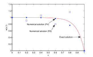
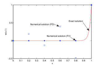
Figure 1: Comparisons between the FV scheme and the FD scheme, the left is for Case 1 and the right for Case 2

References

[1] A. Berman, and R. Plemmons, Nonnegative Matrices in the Mathematical Sciences, Academic Press, New York,
1979.
[2] X. Cao, J. Fu, and H. Huang, Numerical method for the time fractional Fokker Planck
equation, Adv. Appl. Math. Mech., 4(2012), 848-863.
[3] S. Chen, F. Liu, P. Zhuang, and V. Anh, Finite difference approximations for the fractional Fokker-Planck equation, Appl. Math. Model., 33(2009), 256-273.
[4] R. Cottle, J. Pang, and R. Stone, The Linear Complementarity Problem, Academic Press, New York, 1992.
[5] W. Deng, Numerical algorithm for the time fractional Fokker-Planck equation, J. Comput. Phys., 227(2007), 1510-1522.
[6] W. Deng, Finte element method for the space and time fractional fokker-planck equation, SIAM J. Numer. Anal., 47(2008), 204-226.
[7] G. Fairweather, H. Zhang, X. Yang, and D. Xu, A backward Euler orthogonal spline collocation method for the time-fractional, Fokker-Planck equation, Numer. Meth. PDEs.,
31(2015), 1534-1550.
[8] L. B. Feng, P. Zhuang, F. Liu, and I. Turner, Stability and convergence of a new finite
volume method for a two-sided space-fractional diffusion equation, Appl. Math. and
Comput., 257(2015), 52-65.
[9] H. Hejazi, T. Moroney, and F. Liu, A finite volume method for solving the two-sided time-space
fractional advection-dispersion equation, Cent. Eur. J. Phys., 11(2013), 1275-1283.
[10] H. Hejazi, T. Moroney, and F. Liu, Stability and convergence of a finite volume method for
the space fractional advection-dispersion equation, J. Comput. Appl. Math., 255(2014),
684-697.
[11] R. Hilfe, Applications of Fractional Calculus in Physics, World Scientific, Singapore, 1999.
[12] K. Miller, and B. Ross, An Introduction to the Fractional Calculus and Fractional Differential Equations, Wiley, New York, 1993.
[13] Y. Jiang, A new analysis of stability and convergence for finite difference schemes solving the time fractional Fokker-Planck equation, Appl. Math. Model., 39(2015), 1163-1171.
[14] Y. Jiang, and J. Ma, Moving finite element methods for time fractional partial differential equations, Sci. China. Ser. A., 56(2013), 1287-1300.
[15] Y. Jiang, and J. Ma, High-order finite element methods for time-fractional partial
differential equations, J. Comput. Appl. Math., 235(2011), 3285–3290.
[16] S. Karaa, K. Mustapha, and A. K. Pani, Finite volume element method for two-dimensional fractional subdiffusion problems, IMA J. Numer. Anal., 2016. ????
[17] T. Langlands, and B. Henry, The accuracy and stability of an implicit solution method for the fractional diffusion equation, J. Comput. Phys., 205(2005), 719-736.
[18] C. Li, and W. Deng, Remarks on fractional derivatives, Appl. Math. Comput., 187(2007), 777-784.
[19] X. Li, and C. Xu, A space-time spectral method for the time fractional diffusion equation, SIAM J. Numer. Anal., 47(2009), 2108-2131.
[20] Y. Lin, and C. Xu, Finite difference/spectral spproximations for the time-fractional diffusion equation, J. Comput. Phys., 225(2007), 1533-1552.
[21] F. Liu, P. Zhuang, I. Turner, K. Burrage, and V. Anh, A new fractional finite volume
method for solving the fractional diffusion equation, Appl. Math. Modell, 38(2014), 3871-3878.
[22] W. McLean, and K. Mustapha, Convergence analysis of a discontinuous Galerkin method for a sub-diffusion equation, Numer. Algorithms, 5(2009), 69-88.
[23] R. Metzler, E. Barkai, and J. Klafter, Anomalous diffusion and relaxation close to thermal equilibrium: a fractional Fokker-Planck equation approach, Phys. Rev. Lett., 82(1999), 3563-3567.
[24] R. Metzler, and J. Klafter, Le vy meets Boltzmann: strange initial conditions for Brownian and fractional Fokker-Planck equations,
Physica A, 302(2001), 290-296.
[25] K. Mustapha, and M. McLean, Piecewise-linear, discontinous Galerkin method for a fractional diffusion equation, Numer. Algorithms, 56(2011), 159-184.
[26] K. B. Oldham, and J. Spanier, The Fractional Calculus, Academic Press, New York, 1974.
[27] I. Podlubny, Fractional Differential Equations, Academic Press, New York, 1999.
[28] A. Saadatmandi, M. Dehghan, and M. Azizi, The Sinc-Legendre
collocation method for a class of fractional convection-diffusion equations with variable
coefficients, Commun. Nonlinear Sci. Numer. Simul., 17(2012), 4125-4136.
[29] Z. Sheng, and G. Yuan, An improved monotone finite volume scheme for diffusion equation on polygonal meshes,
J. Comput. Phys., 231(2012), 3739-3754.
[30] F. So, and K. L. Liu, A study of the subdiffusive fractional Fokker-Planck equation of bistable systems, Physica A, 331(2004), 378-390.
[31] I. M. Sokolov, A. Blumen, and J. Klafter, Linear response in complex systems: CTRW and the fractional Fokker CPlanck equations,
Physica A, 302(2001), 268-278.
[32] H. K. Versteeg, and W. Malalasekera, An introduction to computational fluid dynamics-the finite volume method,
Longman Scientific and Technical, New York, 1995.
[33] S. Vong, and Z. Wang, A high order compact finite difference scheme for time
fractional Fokker-Planck equations, Appl. Mat. Lett., 43(2015), 38-43.
[34] Q. Yang, I. Turner, T. Moroney, and F. Liu, A finite volume scheme with preconditioned
Lanczos method for two-dimensional space-fractional reaction-diffusion equations, Appl.
Math. Modell., 38(2014), 3755-3762.
[35] P. Zhuang, F. Liu, V. Anh, and I. Turner, New solution and analytical techniques of the implicit numerical method for the anomalous subdiffusion equation, SIAM J. Numer. Anal., 46(2008), 1079-1095.
[36] P. Zhuang, F. Liu, V. Anh, and I. Turner, Stability and convergence of an implicit numerical method for the non-linear fractional reaction-subdiffusion process, IMA J. Numer. Math., 74(2009), 645-667.