Event-Triggered Diffusion Kalman Filters

Abstract

Distributed state estimation strongly depends on collaborative signal processing, which often requires excessive communication and computation to be executed on resource-constrained sensor nodes. To address this problem, we propose an event-triggered diffusion Kalman filter, which collects measurements and exchanges messages between nodes based on a local signal indicating the estimation error. On this basis, we develop an energy-aware state estimation algorithm that regulates the resource consumption in wireless networks and ensures the effectiveness of every consumed resource. The proposed algorithm does not require the nodes to share its local covariance matrices, and thereby allows considerably reducing the number of transmission messages. To confirm its efficiency, we apply the proposed algorithm to the distributed simultaneous localization and time synchronization problem and evaluate it on a physical testbed of a mobile quadrotor node and stationary custom ultra-wideband wireless devices. The obtained experimental results indicate that the proposed algorithm allows saving $86\%$ of the communication overhead associated with the original diffusion Kalman filter while causing deterioration of performance by $16\%$ only. We make the Matlab code and the real testing data available online.

I Introduction

The State estimation algorithms used in wireless sensor networks enable services in various fields, such as emergency rescue, homeland security, military operations, habitat monitoring, and home automation services [1]. In addition to ensuring the accuracy of the state estimation, one has to consider power constraints [2], limitations in terms of bandwidth [3], and limitations in computation [4] and communication [5]. One of the most widely applied estimation algorithms for sensor networks is the distributed Kalman filtering algorithm [6]. Among distributed Kalman filters, diffusion algorithms [7] have favorable properties with respect to performance and robustness in terms of handling node and link failures.

The performance of the diffusion Kalman filters [7] depends on frequent measurements and message exchange between nodes. However, the capabilities of individual nodes are limited, and each node is often battery-powered. Therefore, decreasing communication overhead and the number of measurements is of great importance. The main open question to be considered is not how great estimation an algorithm could achieve, but rather to what extent it is capable of satisfying the application needs while saving resources. To address this question, we propose an event-triggered diffusion Kalman filter that restricts the amount of processing, sensing, and communication based on a local signal indicating an estimation error without requiring the nodes to share their local covariance matrices. Therefore, the number of transmission messages compared to the nominal distributed diffusion Kalman filter algorithm is significantly reduced. In particular, we characterize the trade-off between the consumed resources and the corresponding estimation performance.

As a representative application of distributed state estimation, we consider localization and time synchronization. Maintaining a shared notion of the time is critical for ensuring acceptable performance and robustness of many cyber-physical systems (CPS). Furthermore, position estimation is a crucial task in different fields. Nevertheless, localization and time synchronization algorithms require a significant amount of collaboration efforts between individual sensors, and therefore, the proposed approach is particularly helpful for this application. More specifically, we apply the proposed event-triggered diffusion Kalman filter on D-SLATS [8, 9], which is a distributed simultaneous localization and time synchronization framework.

In the present study, we make the following contributions:

• Introducing the event-triggered distributed diffusion Kalman filter to reduce communication, computational, and sensing overheads.

• Showing that our event-triggered estimator is unbiased and deriving the relationship between the triggering signal and the expected error covariance.

• Applying the proposed strategy in localizing and time-synchronizing of distributed nodes in an ad-hoc network.

• Evaluating the proposed strategy on a real testbed using custom ultra-wideband wireless devices and a quadrotor.

The rest of the paper is organized as follows. Section II provides an overview on the related work. Section III gives the motivation behind our chosen triggering condition. Then, we present the proposed algorithm and corresponding theoretical analysis in Sections IV and V, respectively. Section VI illustrates the application to localization and time synchronization, provides the description of the experimental setup, and evaluates the proposed algorithm on static and mobile networks of nodes. Finally, Section VII summarizes some concluding and discussion remarks.

II Related Work

We first discuss the general state estimation algorithms followed by centralized and distributed event-triggered estimators.

II-A State Estimation Algorithms

Estimation algorithms based on average consensus have been analyzed in [6, 10, 11]. The distributed estimation algorithm proposed in [12] is intended for extremely large-scale systems. The main idea is to approximate the inverse of the large covariance matrix $P$ by using the L-banded inverse and the distributed iterate collapse inversion overrelaxation (DICI-OR) method [13]; however, it requires a large amount of computation resources. Due to limited resources available in wireless sensor networks, many investigations have been made seeking to decrease the communication and computation overheads, while preserving the acceptable performance. This has served as the basis for the studies in the following categories.

II-B Centralized Event-Triggered Estimation Algorithms

The event-triggered scheme has already been applied to network estimation problems. It was first proposed with regard to the centralized estimation problems. The send-on-delta method is proposed for Kalman filters in [14], where the sensor data values are transmitted only upon encountering a user-defined change. An event-triggered sensor data scheduler based on the minimum mean-squared error (MMSE) has been proposed in [15]. In [16], the variance-based triggering scheme has been introduced, implying that each node runs a copy of the Kalman filter and transmits its measurement only if the associated measurement prediction variance exceeds a chosen threshold. The properties of the set-valued Kalman filters with multiple sensor measurements have been analyzed in [17]. Open-loop and closed-loop stochastic event-triggered sensor schedules for remote state estimation have been proposed [18].

In general, the required amount of communication can be reduced by using an event-triggered scheme in which the sensor and estimator are not at the same node, as discussed in [19, 20]. Moreover, a discrete-time approach is proposed in [21] to address the same concern. The importance of considering the effects of external disturbances and measurement noise in the analysis of event-triggered control systems is discussed in [22]. Event-triggered centralized state estimation for linear Gaussian systems is proposed in [23]. Finally, the covariance intersection algorithm is investigated to enable a centralized event-triggered estimator [24].

II-C Distributed Event-Triggered Estimation Algorithms

As one of the main goals of sensor networks is to perform estimation in a distributed manner, event-triggered approaches are also applied in the corresponding distributed scenarios, including Kalman filters with covariance intersection [25]. An event-triggered distributed Kalman filter is proposed in [26] for networked multi-sensor fusion systems with limited bandwidth. An event-triggered consensus Kalman filter with guaranteed stability is proposed in [27]. The authors in [28, 29] propose an event-triggered communication protocol and provide a designing mechanism for triggering thresholds with guaranteed boundedness of the error covariance for distributed Kalman filters with covariance intersection. Notably, the send-on-delta data transmission mechanisms are proposed in the event-triggered Kalman consensus filters [30]. Moreover, event triggering on the sensor-to-estimator and estimator-to-estimator channels are investigated with regard to the distributed Kalman consensus [31]. Transmission delays and data drops in a distributed event-triggered control system are considered in [32]. Moreover, multiple distributed sensor nodes are considered in [33], where the sensors are used to observe a dynamic process and to exchange their measurements sporadically aiming to estimate the full state of the dynamic system. Significant deviation from the information predicted based on the last transmitted information is monitored to obtain a data-driven distributed Kalman filter [25]. For more details on the related work, we refer to the research presented on [34].

It is deemed not efficient to propose an event-triggered diffusion Kalman filter to reduce communication and computational costs and to require sharing the local covariance matrices with the purpose of finding the optimal diffusion weights. Therefore, we focus on event-triggered diffusion Kalman filters without sharing the local covariance matrices. This research direction has two related works. The first one is dedicated to a partial diffusion Kalman filter [35], which is mainly intended to address the diffusion step where Every wireless node shares only a subset of its intermediate estimate vectors among its neighbors at each iteration. However, there is no resource-saving achieved at the measurement update step, which already imposes high communication and sensing overheads. Also, it is not duty cycling the whole communication process within the diffusion step. On the other hand, the concern of the other work [36] is optimizing the measurement update step while neglecting the diffusion step, which is associated with the significant overhead, as shown in [35]. In the present study, we consider both the diffusion and the measurement steps; we temporarily shut-down the sensing and communication between nodes. To the best of our knowledge, the present paper is the first work focused on event-triggering the aforementioned steps of diffusion Kalman filter without the need to share the local covariance matrices. Moreover, we evaluate the proposed mechanism on a real testbed for localization and time synchronization.

III Triggering Logic Motivation

One of the merits of the original centralized Kalman filter is the error covariance matrix. It is deemed as a perfect measure of the expected accuracy of the estimated state and can be utilized for regulating the resource consumption based on the particular application needs. However, when it comes to the distributed diffusion Kalman filter, we do not have local access to the error covariance matrix [7]. Therefore, we aim to obtain the expected accuracy of the estimated state in the distributed diffusion Kalman filter, in which the local estimators do not have access to all measurements. To provide the step-by-step rationale behind the proposed approach, let us start by considering a background example to illustrate the relationship between the global and local covariance information at each node based on the partial access to the measurements, which is the case of distributed filtering.

Example 1.

Let us introduce $\hat{x}_{1}$ as the least-mean-squares estimator of $x$ given a zero-mean observation $y_{1}$, $\hat{x}_{2}$ as the least-mean-squares estimator of $x$ given a zero-mean observation $y_{2}$, and $\hat{x}$ as least-mean-squares estimator of $x$ given all observations. As a consequence, we obtain the two separate estimators for $x$ given two separate measurements and a global estimator given all the measurements. Let $P_{1}$, $P_{2}$ and $P$ denote the corresponding local and global error covariance matrices, respectively. We assume that the measurement noises are uncorrelated and have zero mean. It can be shown [37, p.89] that the global and local error covariance matrices are related as per the following equation

$$P^{-1}=P_{1}^{-1}+P_{2}^{-1}-R_{x},$$ (1)

where $R_{x}$ is the positive-definite covariance matrix of $x$.

In the case of the distributed Kalman filter, every node obtains access to the measurements of its neighbors in addition to its local measurements. Therefore, we introduce two terms: individual and local estimates. The individual estimate considers only the measurements at the node itself without referring to its neighbors, while the local one considers the individual measurements together with those the measurements of its neighbors. More specifically, we denote the individual estimate by $\hat{x}^{\text{ind}}_{k,i|j}$, which corresponds to the optimal linear estimate of $x_{i}$ at time step $i$ given only the individual measurements up to time $j$ at node $k$ without considering its neighbors; and the individual error covariance matrix is denoted by $P^{\text{ind}}_{k,i|j}$. The local estimate at node $k$ is denoted by $\hat{x}^{\text{loc}}_{k,i|j}$ and corresponds to the optimal linear estimate of $x_{i}$ at time step $i$ given its individual measurements and measurements across the neighbors of node $k$ until time step $j$. The local error covariance matrix is denoted by $P^{\text{loc}}_{k,i|j}$. We also denote the global estimate by $\hat{x}_{i|j}$, which corresponds to the optimal linear estimate of $x_{i}$ given all observations across all nodes up to time step $j$ and its error covariance matrix by $P_{i|j}$.

The global error covariance matrix $P_{i|i}$ denotes the expected estimation error. Therefore, we can duty cycle collecting measurements and message exchange processes based on a threshold on the trace of the global error covariance matrix $P_{i|i}$. However, in the distributed Kalman filter algorithms, every node has access only to its local matrix $P^{\text{loc}}_{k,i|i}$ in distributed Kalman filter algorithms and does not have access to $P_{i|i}$ locally. Therefore, let us investigate if there is a direct relation between $P_{i|i}$ and $P^{\text{loc}}_{k,i|i}$. Instead of considering two nodes, we extend (1) to $N$ nodes where every node uses its individual measurements only [38, p.14] as follows:

$$P_{i|i}^{-1}=\sum\limits_{k=1}^{N}(P^{\text{ind}}_{k,i|i})^{-1}-(N-1)\Pi^{-1}_{i},$$ (2)

where $\Pi_{i}$ is the covariance matrix of $x_{i}$. The individual error covariance matrices $P^{\text{ind}}_{k,i|i}$ are expected to decrease over time in observable systems. Therefore, their inverses in the first term $\sum\limits_{k=1}^{N}(P^{\text{ind}}_{k,i|i})^{-1}$ in (2) become dominant. Therefore, $P_{i|i}^{-1}$ can be approximated as follows:

$$P_{i|i}^{-1}\approx\sum\limits_{k=1}^{N}(P^{\text{ind}}_{k,i|i})^{-1}.$$ (3)

Then, let us apply (1) while sharing the measurements between the neighbors, i.e, considering the local estimates. We can find that the local error covariance $P^{\text{loc}}_{k,i|i}$ of each node $k$ depends on $P^{\text{ind}}_{l,i|i}$ of each neighbor $l$ as the local estimation process considers the neighbors measurements. Therefore, we can relate $P^{\text{loc}}_{k,i|i}$ to $P^{\text{ind}}_{k,i|i}$ in (4) with the aid of the adjacency matrix $A$ which has unity entry if the corresponding nodes are neighbors, and zero otherwise. Here $a_{l,k}$ denotes the element at row $l$ and column $k$ of matrix $A$ [38, p.14].

$$(P^{\text{loc}}_{k,i|i})^{-1}=\sum\limits_{l=1}^{N}a_{l,k}(P^{\text{ind}}_{l,i|i})^{-1}-\Big{(}\sum\limits_{l=1}^{N}a_{l,k}-1\Big{)}\Pi^{-1}_{i},$$ (4)

where

$$a_{l,k}=\begin{cases}1&\text{if }l\in\mathscr{N}_{k},\\ 0&\text{otherwise}.\end{cases}$$ (5)

If we sum up (4) for all $N$ nodes with a set of real weights $\gamma_{k}$ associated with every node $k$, we obtain the following combinations:

$$\sum\limits_{k=1}^{N}\gamma_{k}(P^{\text{loc}}_{k,i|i})^{-1} = \sum\limits_{l=1}^{N}\sum\limits_{k=1}^{N}\gamma_{k}a_{l,k}(P^{\text{ind}}_{l,i|i})^{-1}$$ (6)

$$-\Big{(}\sum\limits_{l=1}^{N}\sum\limits_{k=1}^{N}\gamma_{k}a_{l,k}-\sum\limits_{k=1}^{N}\gamma_{k}\Big{)}\Pi^{-1}_{i}.$$

Setting the weights in (6) such that $\sum\limits_{k=1}^{N}\gamma_{k}a_{l,k}=1$ for all $l$, and having the first term again on the right-hand side dominant, as the individual error covariance matrices are expected to get smaller with time, results in

$$\sum\limits_{k=1}^{N}\gamma_{k}(P^{\text{loc}}_{k,i|i})^{-1}\approx\sum\limits_{l=1}^{N}(P^{\text{ind}}_{l,i|i})^{-1}.$$ (7)

Equating the two approximations in (7) and (3) results in

$$P_{i|i}^{-1}\approx\sum\limits_{k=1}^{N}\gamma_{k}(P^{\text{loc}}_{k,i|i})^{-1}.$$ (8)

We have shown direct approximation between the matrix $P_{i|i}$ and local available matrix $P^{\text{loc}}_{k,i|i}$. Therefore, we can trigger collecting measurements based on the trace of the local error covariance matrix $P^{\text{loc}}_{k,i|i}$, which is available in distributed Kalman filters. This is the motivation behind the triggering logic considered in the present study.

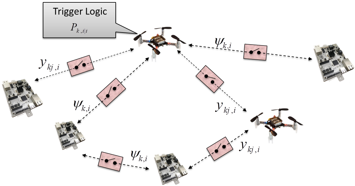
Figure 1: Every sensor node runs a distributed event-triggered state estimator to obtain the network state $x_{k,i|i}$. The nodes only share the measurements $y_{kj,i}$ and intermediate estimates $\Psi_{j,i}$ with their neighbors.

IV Event-Triggered Diffusion Extended Kalman Filter Algorithm

We consider the event-triggered distributed state estimation problem over a network of $N$ distributed nodes indexed by $k\in\{0,\ldots,N-1\}$ as shown in Figure 1. Each node represents a sensor and an estimator. Moreover, we consider that two nodes are connected if they can communicate directly with each other. Let us consider the following nonlinear time-varying system to fit our nonlinear application as follows:

$$\begin{split}x_{i+1}&=f_{i}(x_{i})+G_{i}n_{i}\\ y_{kj,i}&=h_{k,i}(x_{i})+v_{k,i}\\ \end{split}$$ (9)

where $x_{i}\in\mathbb{R}^{m}$ is the state at time step $i$ and $y_{kj,i}\in\mathbb{R}^{L_{k}}$ is the measurement between node $k$ and its neighbor node $j$ $\in$ $\mathscr{N}_{k}$ at time step $i$. Furthermore, the process noise $n_{i}$ and the measurement noise $v_{k,i}$ are assumed to be uncorrelated, and zero mean white Gaussian noises. The matrices $Q_{i}$ and $R_{i}$ are the process and the measurement covariance matrices at time step $i$, respectively. The state update and measurement functions are denoted by $f_{i}$ and $h_{k,i}$, respectively.

We denote the estimate at time step $i$ of $x_{i}$ by $\hat{x}_{k,i|s}$ given the observations up to time $s$ at node $k$, when every node seeks to minimize the mean squared error $\mathbb{E}\|x_{i}-\hat{x}_{k,i|i}\|^{2}$. To handle the nonlinearity in the considered model, we linearize (9) at a linearization point $z$, and apply the diffusion Kalman filtering algorithm [7, 38]. The resulting state update and measurement functions are shown in (10) and (11). The linearization clearly depends on $z$, and this point should be the best available local estimate of $x_{i}$:

$$\bar{F}_{i}(z) \mathrel{:=}\frac{\partial f_{i}(x)}{\partial x}\Big{\rvert}_{x=z},$$ (10)

$$\bar{H}_{k,i}(z) \mathrel{:=}\frac{\partial h_{k,i}(x)}{\partial x}\Big{\rvert}_{x=z}.$$ (11)

Given a linearized model, we subsequently explain the proposed event-triggered diffusion extended Kalman filter algorithm shown in Algorithm $1$. One of the nodes is elected beforehand as a leader based on the accessibility of important measurements, which facilitates reaching the best local estimate compared to the followers. We denote the leader node by subscript $L$ and its job to take the duty-cycling decision. Choosing a proper leader is crucial in saving energy; however, the election process based on the available estimates is out of scope of this paper. Algorithm $1$ is started with the measurement update (step 1), in which every node $k$ obtains a local estimate $\Psi_{k,i}$ at time step $i$. Then, information from the neighbors of node $k$ is diffused in a convex combination to produce a better new state estimate in step $2$. The $c_{k,j}$ elements represent the weights that are used by the diffusion algorithm to combine neighboring estimates. Step 1 and 2 are only executed if the trace of the required part of the leader matrix $P_{L,i|i-1}$ is greater than the user-defined threshold $\pi_{\max}$. Explicitly, the triggering event is defined as $\operatorname{\mathsf{tr}}(WP_{L,i|i-1}W^{\operatorname{\mathsf{T}}})>\pi_{\max}$, where $W$ is a weighting matrix to choose the required part of $P_{L,i|i-1}$. If the triggering event is not satisfied, we do not take measurements $y_{kj,i}$, and we save the communication costs at steps $1$ and $2$. Instead, we perform the propagation update (step $3$), in which every node considers the new estimates as the old available ones $\hat{x}_{k,i|i}=\hat{x}_{k,i|i-1}$ and its corresponding local matrix $P_{k,i|i}=P_{k,i|i-1}$. Finally, every node performs the time update (step 4) in all cases.

It should be noted that the analysis presented in Section III shows the relationship between the global error covariance and the available local error covariance during the measurement update (step 1) in Algorithm $1$. However, the diffusion update (step 2) does not take into account recursions for these local error covariance matrices as it only combines the estimates of the neighbors without considering their local error covariance matrices. Moreover, exchanging the $P^{\text{loc}}_{k,i|i}$ between neighbors to maintain the exact expected estimation error is of a great overhead in sensor networks. Furthermore, the diffusion step decreases the estimation error so that it should be included. Therefore, we continue with the modified version of $P^{\text{loc}}_{k,i|i}$, which we call diffusion error covariance matrix, and denote it by $P_{k,i|i}$ in Algorithm $1$.

1

Algorithm 1 Event-Triggered Diffusion Extended Kalman Filter

Start with $\hat{x}_{k,0|-1}=x_{0}$ and $P_{k,0|-1}=\Pi_{0}$ for all $k$, and at every time instant $i$, compute at every node $k$:

2 if $\operatorname{\mathsf{tr}}(WP_{L,i|i-1}W^{T})>\pi_{\max}$ then

3       Step 1: Measurement update:

$$\hat{H}_{kj,i} = \bar{H}_{j,i}(\hat{x}_{k,i|i-1})$$ (12)

$$P^{-1}_{k,i|i} = P^{-1}_{k,i|i-1}+\sum\limits_{j\in\mathscr{N}_{k}}\hat{H}_{kj,i}^{T}{R}^{-1}_{i}\hat{H}_{kj,i}$$ (13)

$$\Psi_{k,i} = \hat{x}_{k,i|i-1}$$

$$+P_{k,i|i}\sum\limits_{j\in\mathscr{N}_{k}}\hat{H}^{T}_{kj,i}R_{i}^{-1}[y_{kj,i}-h_{j,i}(\hat{x}_{k,i|i-1})]$$

Step 2: Diffusion update:

$$\hat{x}_{k,i|i} = \sum\limits_{j\in\mathscr{N}_{k}}c_{k,j}\Psi_{j,i}$$ (15)

4else

5       Step 3: Propagation update:

$$\hat{x}_{k,i|i} = \hat{x}_{k,i|i-1}$$ (16)

$$P_{k,i|i} = P_{k,i|i-1}$$ (17)

Step 4: Time update:

$$\hat{x}_{k,i+1|i} = f_{i}(\hat{x}_{k,i|i})$$ (18)

$$P_{k,i+1|i} = \bar{F}_{i}(\hat{x}_{k,i|i})P_{k,i|i}\bar{F}_{i}^{T}(\hat{x}_{k,i|i})+G_{i}Q_{i}G_{i}^{T}$$ (19)

V Theoretical Analysis

We limit our analysis to the linear case. We prove that event-triggered diffusion Kalman is an unbiased estimator. Next, we show the relationship between the local matrix $P_{k,i|i}$ and the augmented error covariance. Let us consider the following linear time-varying system

$$x_{i+1} =F_{i}x_{i}+G_{i}n_{i},$$ (20)

$$y_{kj,i} =H_{k,i}x_{i}+v_{k,i}.$$ (21)

Lemma 1.

The event-triggered diffusion Kalman filter is an unbiased estimator.

Proof.

The measurement update step in the linear case results in the following (linear version of (13), (3)):

$$P^{-1}_{k,i|i} =P^{-1}_{k,i|i-1}+\sum\limits_{j\in\mathscr{N}_{k}}H_{j,i}^{T}{R}^{-1}_{i}H_{j,i},$$ (22)

$$\Psi_{k,i} =\hat{x}_{k,i|i-1}+P_{k,i|i}\sum\limits_{j\in\mathscr{N}_{k}}H^{T}_{j,i}R_{i}^{-1}[y_{kj,i}-H_{j,i}\hat{x}_{k,i|i-1}].$$ (23)

The estimation error $\tilde{x}_{k,i|i-1}$ at the end of Algorithm $1$ is defined and updated according to the formula:

$$\tilde{x}_{k,i|i-1} \mathrel{:=}x_{i}-\hat{x}_{k,i|i-1}$$

$$=F_{i-1}\tilde{x}_{k,i-1|i-1}+G_{i-1}n_{i-1}.$$ (24)

After defining the estimation error at the end of the measurement update by $\tilde{\Psi}_{k,i}$, we obtain that:

$$\tilde{\Psi}_{k,i} \mathrel{:=} x_{i}-\Psi_{k,i}$$ (25)

$$\stackrel{{\scriptstyle\eqref{equ:psi}}}{{=}} \tilde{x}_{k,i|i-1}-P_{k,i|i}\sum\limits_{j\in\mathscr{N}_{k}}H^{T}_{j,i}R_{i}^{-1}\Big{[}y_{kj,i}-H_{j,i}(x_{i}-\tilde{x}_{k,i|i-1})\Big{]}$$

$$\stackrel{{\scriptstyle\eqref{equ:ylinear}}}{{=}} \tilde{x}_{k,i|i-1}-P_{k,i|i}\sum\limits_{j\in\mathscr{N}_{k}}H^{T}_{j,i}R_{i}^{-1}\Big{[}H_{j,i}\tilde{x}_{k,i|i-1}+v_{j,i}\Big{]}$$

$$= P_{k,i|i}\Big{(}P_{k,i|i}^{-1}-\sum\limits_{j\in\mathscr{N}_{k}}H^{T}_{j,i}R_{i}^{-1}H_{j,i}\Big{)}\tilde{x}_{k,i|i-1}$$

$$-P_{k,i|i}\sum\limits_{j\in\mathscr{N}_{k}}H^{T}_{j,i}R_{i}^{-1}v_{j,i}.$$

Using (22) to simplify (25) results in the following:

$$\tilde{\Psi}_{k,i}\stackrel{{\scriptstyle\eqref{equ:pinv}}}{{=}}P_{k,i|i}P_{k,i|i-1}^{-1}\tilde{x}_{k,i|i-1}-P_{k,i|i}\sum\limits_{j\in\mathscr{N}_{k}}H^{T}_{j,i}R_{i}^{-1}v_{j,i}.$$ (26)

Applying the diffusion step (15) results in

$$\tilde{x}_{\scriptscriptstyle k,i|i} =\sum_{l\in\mathscr{N}_{k}}c_{l,k}\tilde{\Psi}_{l,i}$$

$$\stackrel{{\scriptstyle\eqref{equ:psierr2}}}{{=}}\sum_{l\in\mathscr{N}_{k}}c_{l,k}\bigg{[}P_{\scriptscriptstyle l,i|i}P_{\scriptscriptstyle l,i|i-1}^{-1}\tilde{x}_{\scriptscriptstyle l,i|i-1}-P_{\scriptscriptstyle l,i|i}\sum\limits_{j\in\mathscr{N}_{l}}H^{T}_{j,i}R_{i}^{-1}v_{j,i}\bigg{]}.$$ (27)

Executing $M$ time updates and propagation updates before $\operatorname{\mathsf{tr}}(WP_{L,i|i}W^{T})$ exceeds the threshold $\pi_{\max}$ results in the following:

$$\tilde{x}_{\scriptscriptstyle k,i+M+1|i+M} \stackrel{{\scriptstyle\eqref{equ:xerrupdate}}}{{=}} F_{\scriptscriptstyle i+M}\tilde{x}_{\scriptscriptstyle k,i+M|i+M}+G_{\scriptscriptstyle i+M}n_{\scriptscriptstyle i+M}$$

$$\stackrel{{\scriptstyle\eqref{equ:x_propupdate}}}{{=}} F_{\scriptscriptstyle i+M}\tilde{x}_{\scriptscriptstyle k,i+M|i+M-1}+G_{\scriptscriptstyle i+M}n_{\scriptscriptstyle i+M}$$

$$\stackrel{{\scriptstyle\eqref{equ:xerrupdate}}}{{=}} F_{\scriptscriptstyle i+M}\Big{(}F_{\scriptscriptstyle i+M-1}\tilde{x}_{\scriptscriptstyle k,i+M-1|i+M-1}$$

$$+G_{\scriptscriptstyle i+M-1}n_{\scriptscriptstyle i+M-1}\Big{)}+G_{\scriptscriptstyle i+M}n_{\scriptscriptstyle i+M}.$$

After using (24) and (16) multiple times to obtain $\tilde{x}_{\scriptscriptstyle k,i+M+1|i+M}$ as a function of $\tilde{x}_{\scriptscriptstyle k,i|i}$, we obtain that:

$$\tilde{x}_{\scriptscriptstyle k,i+M+1|i+M} = \prod_{j=0}^{M}F_{\scriptscriptstyle i+M-j}\tilde{x}_{\scriptscriptstyle k,i|i}+\sum_{l=1}^{M}\prod_{j=0}^{M-l}F_{\scriptscriptstyle i+M-j}G_{\scriptscriptstyle i+l-1}n_{i+l-1}$$ (28)

$$+G_{\scriptscriptstyle i+M}n_{\scriptscriptstyle i+M}.$$

Inserting (27) in (28) results in

$$\tilde{x}_{\scriptscriptstyle k,i+M+1|i+M}= \prod_{j=0}^{M}F_{\scriptscriptstyle i+M-j}\Bigg{[}\sum_{l\in\mathscr{N}_{k}}c_{\scriptscriptstyle l,k}\bigg{[}P_{\scriptscriptstyle l,i|i}P_{\scriptscriptstyle l,i|i-1}^{-1}\tilde{x}_{\scriptscriptstyle l,i|i-1}$$

$$-P_{\scriptscriptstyle l,i|i}\sum\limits_{j\in\mathscr{N}_{l}}H^{T}_{\scriptscriptstyle j,i}R_{\scriptscriptstyle i}^{-1}v_{\scriptscriptstyle j,i}\bigg{]}\Bigg{]}$$

$$+\sum_{l=1}^{M}\prod_{j=0}^{\scriptscriptstyle M-l}F_{\scriptscriptstyle i+M-j}G_{\scriptscriptstyle i+l-1}n_{\scriptscriptstyle i+l-1}+G_{\scriptscriptstyle i+M}n_{\scriptscriptstyle i+M}.$$ (29)

Taking the expectations of both sides of (29) leads to in the following recursion given that we have zero mean noises:

$$\mathbb{E}\tilde{x}_{\scriptscriptstyle k,i+M+1|i+M}=\prod_{j=0}^{M}F_{\scriptscriptstyle i+M-j}\sum_{l\in\mathscr{N}_{k}}c_{\scriptscriptstyle l,k}P_{\scriptscriptstyle l,i|i}P_{\scriptscriptstyle l,i|i-1}^{-1}\mathbb{E}\tilde{x}_{\scriptscriptstyle l,i|i-1}.$$ (30)

Since $\mathbb{E}\tilde{x}_{l,0|-1}=0$ as $\hat{x}_{l,0|-1}=0$ and $\mathbb{E}x_{0}=0$ [38], we conclude that the event-triggered diffusion Kalman is an unbiased estimator. ∎

The diffusion step (15) in Algorithm 1 combines the intermediate estimates from neighbors without combining the corresponding error covariance matrices, as we mentioned before. Therefore, we need to identify the new relationship between $P_{k,i|i}$, and the augmented error covariance. We define the augmented state-error vector $\tilde{\mathscr{X}}_{i|i}$ for the whole network as follows:

$$\tilde{\mathscr{X}}_{\scriptscriptstyle i|i}\mathrel{:=}\begin{bmatrix}\tilde{x}_{\scriptscriptstyle 1,i|i},\ldots,\tilde{x}_{\scriptscriptstyle N,i|i}\end{bmatrix}^{T}.$$ (31)

The Kronecker product and vector of ones are denoted by $\otimes$ and 1, respectively. The identity matrix of the size $N\times N$ is denoted by $I_{N}$. We further introduce the following block-diagonal matrices and $v_{i}$:

$$\mathscr{H}_{i} \mathrel{:=}\operatorname{\mathsf{diag}}(H_{\scriptscriptstyle 1,i},\dots,H_{\scriptscriptstyle N,i}),$$

$$\mathscr{P}_{\scriptscriptstyle i|i} \mathrel{:=}\operatorname{\mathsf{diag}}(P_{\scriptscriptstyle 1,i|i},\dots,P_{\scriptscriptstyle N,i|i}),$$

$$\mathscr{P}_{\scriptscriptstyle i|i-1} \mathrel{:=}\operatorname{\mathsf{diag}}(P_{\scriptscriptstyle 1,i|i-1},\dots,P_{\scriptscriptstyle N,i|i-1}),$$

$$v_{\scriptscriptstyle i} \mathrel{:=}[v_{\scriptscriptstyle 1,i},\ldots,v_{\scriptscriptstyle N,i}]^{T}.$$

Lemma 2.

The relationship between the error covariance $\mathscr{P}_{\scriptscriptstyle\tilde{\mathscr{X}}|i}=\mathbb{E}(\tilde{\mathscr{X}}_{\scriptscriptstyle i|i}\tilde{\mathscr{X}}_{\scriptscriptstyle i|i}^{T})$ of the augmented state and the diffusion error covariance $P_{k,i|i}$ is defined as follows:

$$\mathscr{P}_{\scriptscriptstyle\tilde{\mathscr{X}}|i+M+1} =A_{\scriptscriptstyle i}\mathscr{P}_{\scriptscriptstyle\tilde{\mathscr{X}}|i}A_{\scriptscriptstyle i}^{T}+B_{i}\big{(}\text{1}\text{1}^{T}\otimes Q_{\scriptscriptstyle i+M}\big{)}B_{\scriptscriptstyle i}^{T}$$

$$+\sum_{l=1}^{M}D_{\scriptscriptstyle i,l}\big{(}\text{1}\text{1}^{T}\otimes Q_{\scriptscriptstyle i+l-1}\big{)}D_{\scriptscriptstyle i,l}^{T}+E_{\scriptscriptstyle i}R_{\scriptscriptstyle i+M+1}E_{\scriptscriptstyle i}^{T},$$ (32)

where

$$Z_{\scriptscriptstyle i} \mathrel{:=}\mathscr{C}^{T}\mathscr{P}_{\scriptscriptstyle i+M+1|i+M+1}\mathscr{P}_{\scriptscriptstyle i+M+1|i+M}^{-1},$$

$$A_{\scriptscriptstyle i} \mathrel{:=}Z_{\scriptscriptstyle i}\big{(}I_{\scriptscriptstyle N}\otimes\prod_{j=0}^{M}F_{\scriptscriptstyle i+M-j}\big{)},$$

$$B_{\scriptscriptstyle i} \mathrel{:=}Z_{\scriptscriptstyle i}\big{(}I_{\scriptscriptstyle N}\otimes G_{\scriptscriptstyle i+M}\big{)},$$

$$D_{i,l} \mathrel{:=}Z_{\scriptscriptstyle i}\big{(}I_{\scriptscriptstyle N}\otimes\prod_{j=0}^{\scriptscriptstyle M-l}F_{\scriptscriptstyle i+M-j}\big{)}\big{(}I_{\scriptscriptstyle N}\otimes G_{\scriptscriptstyle i+l-1}\big{)},$$

$$E_{\scriptscriptstyle i} \mathrel{:=}\mathscr{C}^{T}\mathscr{P}_{\scriptscriptstyle i+M+1|i+M+1}\mathscr{A}^{T}\mathscr{H}^{T}_{\scriptscriptstyle i+M+1}\mathscr{R}_{\scriptscriptstyle i+M+1}^{-1}.$$ (33)

Proof.

Extending (27) to the augmented version results in

$$\tilde{\mathscr{X}}_{\scriptscriptstyle i+M+1|i+M+1}\stackrel{{\scriptstyle\eqref{equ:xaug}}}{{=}} \begin{bmatrix}\tilde{x}_{\scriptscriptstyle 1,i+M+1|i+M+1},\ldots,\tilde{x}_{\scriptscriptstyle N,i+M+1|i+M+1}\end{bmatrix}^{T}$$

$$\stackrel{{\scriptstyle\eqref{equ:differr}}}{{=}} \mathscr{C}^{T}\begin{bmatrix}P_{\scriptscriptstyle 1,i+M+1|i+M+1}P_{\scriptscriptstyle 1,i+M+1|i+M}^{-1}\tilde{x}_{\scriptscriptstyle 1,i+M+1|i+M}\\ \vdots\\ P_{\scriptscriptstyle N,i+M+1|i+M+1}P_{\scriptscriptstyle N,i+M+1|i+M}^{-1}\tilde{x}_{\scriptscriptstyle N,i+M+1|i+M}\end{bmatrix}$$

$$-\mathscr{C}^{T}\mathscr{P}_{\scriptscriptstyle i|i}\mathscr{A}^{T}\begin{bmatrix}H_{\scriptscriptstyle 1,i+M+1}R_{\scriptscriptstyle 1,i+M+1}^{-1}v_{\scriptscriptstyle 1,i+M+1}\\ \vdots\\ H_{\scriptscriptstyle N,i+M+1}R_{\scriptscriptstyle 1,i+M+1}^{-1}v_{\scriptscriptstyle N,i+M+1}\end{bmatrix},$$

or equivalently

$$\tilde{\mathscr{X}}_{\scriptscriptstyle i+M+1|i+M+1}= {\ }\mathscr{C}^{T}\mathscr{P}_{\scriptscriptstyle i+M+1|i+M+1}\Big{(}\mathscr{P}_{\scriptscriptstyle i+M+1|i+M}^{-1}\tilde{\mathscr{X}}_{\scriptscriptstyle i+M+1|i+M}$$

$$-\mathscr{A}^{T}\mathscr{H}^{T}_{\scriptscriptstyle i+M+1}\mathscr{R}_{\scriptscriptstyle i+M+1}^{-1}v_{\scriptscriptstyle i+M+1}\Big{)}.$$ (34)

with

$$\mathscr{C}\mathrel{:=}C\otimes I_{m}\quad\quad\mathscr{A}\mathrel{:=}A\otimes I_{m},$$ (35)

where the element at row $l$ and column $k$ of diffusion matrix $C$ is $c_{\scriptscriptstyle l,k}$ in (15). The adjacency matrix is defined as $A$ in (5). The size of $x_{i}$ in (9) is $m$. Similarly, extending (28) to the augmented version results in the following:

$$\tilde{\mathscr{X}}_{\scriptscriptstyle i+M+1|i+M} =\big{(}I_{\scriptscriptstyle N}\otimes\prod_{j=0}^{M}F_{\scriptscriptstyle i+M-j}\big{)}\tilde{\mathscr{X}}_{i|i}+\big{(}I_{\scriptscriptstyle N}\otimes G_{\scriptscriptstyle i+M}\big{)}\big{(}\text{1}\otimes n_{\scriptscriptstyle i+M}\big{)}$$

$$+\sum_{l=1}^{M}\big{(}I_{\scriptscriptstyle N}\otimes\prod_{j=0}^{M-l}F_{\scriptscriptstyle i+M-j}\big{)}\big{(}I_{\scriptscriptstyle N}\otimes G_{\scriptscriptstyle i+l-1}\big{)}\big{(}\text{1}\otimes n_{\scriptscriptstyle i+l-1}\big{)}.$$ (36)

Inserting (36) into (34) leads to the following:

$$\tilde{\mathscr{X}}_{\scriptscriptstyle i+M+1|i+M+1} = A_{\scriptscriptstyle i}\tilde{\mathscr{X}}_{\scriptscriptstyle i|i}+B_{\scriptscriptstyle i}\big{(}\text{1}\otimes n_{\scriptscriptstyle i+M}\big{)}$$ (37)

$$+\sum_{l=1}^{M}D_{\scriptscriptstyle i,l}\big{(}\text{1}\otimes n_{\scriptscriptstyle i+l-1}\big{)}-E_{\scriptscriptstyle i}v_{\scriptscriptstyle i+M+1}.$$

Taking the expectation of both sides of (37) results in (38) with the assumption that the state error $\tilde{\mathscr{X}}$, the time instances of modeling noise $n_{i}$, and the time instances of measurements noise $v_{i}$ are mutually independent [38].

$$\mathscr{P}_{\tilde{\scriptscriptstyle\mathscr{X}}|i+M+1}= {\ }\mathbb{E}\Big{(}\tilde{\mathscr{X}}_{\scriptscriptstyle i+M+1|i+M+1}\tilde{\mathscr{X}}_{\scriptscriptstyle i+M+1|i+M+1}^{T}\Big{)}$$

$$\stackrel{{\scriptstyle\eqref{equ:ximfinal}}}{{=}} A_{\scriptscriptstyle i}\mathbb{E}\Big{(}\tilde{\mathscr{X}}_{\scriptscriptstyle i|i}\tilde{\mathscr{X}}_{\scriptscriptstyle i|i}^{T}\Big{)}A_{\scriptscriptstyle i}^{T}+B_{\scriptscriptstyle i}\mathbb{E}\Big{(}\big{(}\text{1}\otimes n_{\scriptscriptstyle i+M}\big{)}\big{(}\text{1}\otimes n_{\scriptscriptstyle i+M}\big{)}^{T}\Big{)}B_{\scriptscriptstyle i}^{T}$$

$$+\sum_{l=1}^{M}D_{\scriptscriptstyle i,l}\mathbb{E}\Big{(}\big{(}\text{1}\otimes n_{\scriptscriptstyle i+l-1}\big{)}\big{(}\text{1}\otimes n_{\scriptscriptstyle i+l-1}\big{)}^{T}\Big{)}D_{\scriptscriptstyle i,l}^{T}$$

$$+E_{\scriptscriptstyle i}\mathbb{E}\Big{(}v_{\scriptscriptstyle i+M+1}v_{\scriptscriptstyle i+M+1}^{T}\Big{)}E_{\scriptscriptstyle i}^{T}.$$ (38)

Applying the property of Kronecker products that $(A\otimes B)(C\otimes D)^{T}=(AC^{T}\otimes BD^{T})$ results in

$$\mathscr{P}_{\tilde{\scriptscriptstyle\mathscr{X}}|i+M+1}= A_{i}\mathscr{P}_{\tilde{\scriptscriptstyle\mathscr{X}}|i}A_{i}^{T}+B_{i}\big{(}\text{1}\text{1}^{T}\otimes Q_{\scriptscriptstyle i+M}\big{)}B_{\scriptscriptstyle i}^{T}$$

$$+\sum_{l=1}^{M}D_{\scriptscriptstyle i,l}\big{(}\text{1}\text{1}^{T}\otimes Q_{\scriptscriptstyle i+l-1}\big{)}D_{\scriptscriptstyle i,l}^{T}+E_{i}R_{\scriptscriptstyle i+M+1}E_{\scriptscriptstyle i}^{T}.$$ (39)

The above formula connects the error covariance $\mathscr{P}_{\tilde{\mathscr{X}}|i}$ of the augmented state and the diffusion error covariance matrix $P_{k,i|i}$ embedded in $\mathscr{P}_{\scriptscriptstyle i|i}$ and this concludes the proof. ∎

VI Evaluation

In this section, we initiate with describing the application of the proposed approach to the considered localization and time synchronization problem. Thereafter, we present the experimental setup, in which we conducted the experiments. Finally, we perform case studies to obtain equitable evaluation results.

VI-A Application to Localization and Time Synchronization

One of the illustrative applications of the event-triggering body of work is the distributed localization and time synchronization problem, due to its excessive communication and computational overhead. Therefore, we consider this application to demonstrate the practicality of the proposed algorithm. The state vector consists of the three-dimensional position vector $\bm{p}_{k,i}$, the clock time offset $o_{k,i}$, and the clock frequency bias $b_{k,i}$ for all nodes. We adopt convention in which both $o_{k,i}$ and $b_{k,i}$ are described with respect to the global time clock, which is usually the clock of the leader node. Every node is interested in obtaining the state of the whole network. Therefore, the state vector is $x_{\scriptscriptstyle k,i}=[\bar{x}_{\scriptscriptstyle 1,i},...,\bar{x}_{\scriptscriptstyle N,i}]^{T}$, where $\bar{x}_{\scriptscriptstyle k,i}=\left[\bm{p}_{\scriptscriptstyle k,i}^{T},\>o_{\scriptscriptstyle k,i},\>b_{\scriptscriptstyle k,i}\right]^{T}$.

The clock parameters evolve according to the first-order affine approximation of the dynamics $o_{\scriptscriptstyle k,i+1}=o_{\scriptscriptstyle k,i}+b_{\scriptscriptstyle k,i}\delta_{i}$ and $b_{\scriptscriptstyle k,i+1}=b_{\scriptscriptstyle k,i}$, where $\delta_{i}\mathrel{:=}t_{\scriptscriptstyle L,i+1}-t_{\scriptscriptstyle L,i}$ given that $t_{\scriptscriptstyle L,i}$ is the time according to the leader node, which is the global time. Therefore, we can define the update function as follows:

$$f_{i}(\bar{x}_{\scriptscriptstyle k,i}) = \begin{bmatrix}\bm{p}_{\scriptscriptstyle k,i}\\ o_{\scriptscriptstyle k,i}+b_{\scriptscriptstyle k,i}\delta_{\scriptscriptstyle i}\\ b_{\scriptscriptstyle k,i}\end{bmatrix}.$$ (40)

The proposed framework supports the three types of measurements which are distinguished by the number of messages exchanged between a pair of nodes. The measurement vector sent from node $j\in\mathscr{N}_{k}$ to node $k$ has the form $y_{\scriptscriptstyle kj,i}=\left[d_{\scriptscriptstyle kj,i},r_{\scriptscriptstyle kj,i},\Gamma_{\scriptscriptstyle kj,i}\right]^{T}$, where, $d_{\scriptscriptstyle kj,i}$, represents the counter difference at time step $i$ which is the difference between the clock offsets of the two nodes $k$ and $j$. In turn, $r_{\scriptscriptstyle kj,i}$ represents a noisy measurement due to frequency bias discrepancies between $k$ and $j$, which is formally represented by single-sided two-way range. Finally, $\Gamma_{\scriptscriptstyle kj,i}$ is another distance measurement between nodes $k$ and $j$ based on a trio of messages between the nodes at time index $i$. This is a more accurate estimate than $r_{\scriptscriptstyle kj,i}$ owing to the mitigation of frequency bias errors from the additional message. It is formally called double-sided two-way range [8]. We note that a subset of these measurements may be used rather than the full set, i.e., we can conduct experiments involving only $r_{\scriptscriptstyle kj,i}$, $\Gamma_{\scriptscriptstyle kj,i}$, or $d_{\scriptscriptstyle kj,i}$. The response time duration between the first pair of timestamps is denoted by $T_{\scriptscriptstyle RSP1}$. The measurement function is defined as follows [8]:

$$h_{\scriptscriptstyle k,i}(\bar{x}_{\scriptscriptstyle j,i}) =\left[\begin{array}[]{c}\left(o_{\scriptscriptstyle j,i}-o_{\scriptscriptstyle k,i}\right)+\frac{1}{c}\left\|\bm{p}_{\scriptscriptstyle j,i}-\bm{p}_{\scriptscriptstyle k,i}\right\|_{\scriptscriptstyle 2}\\ \left\|\bm{p}_{\scriptscriptstyle j,i}-\bm{p}_{\scriptscriptstyle k,i}\right\|_{2}+\frac{c}{2}\left(b_{\scriptscriptstyle j,i}-b_{\scriptscriptstyle k,i}\right)T_{\scriptscriptstyle RSP1}\\ \left\|\bm{p}_{\scriptscriptstyle j,i}-\bm{p}_{\scriptscriptstyle k,i}\right\|_{\scriptscriptstyle 2}+c\tilde{\Gamma}_{\scriptscriptstyle kj,i}\\ \end{array}\right]$$ (44)

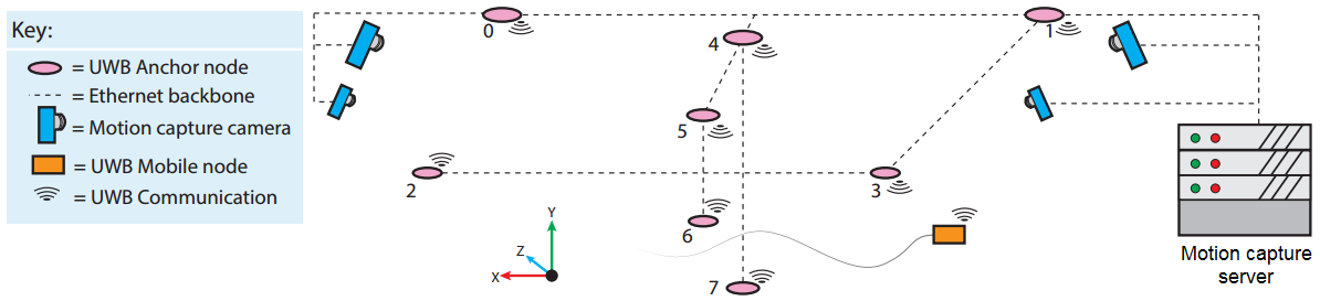
Figure 2: Experimental setup, including, UWB anchor nodes, motion capture cameras, and UWB quadrotor nodes.

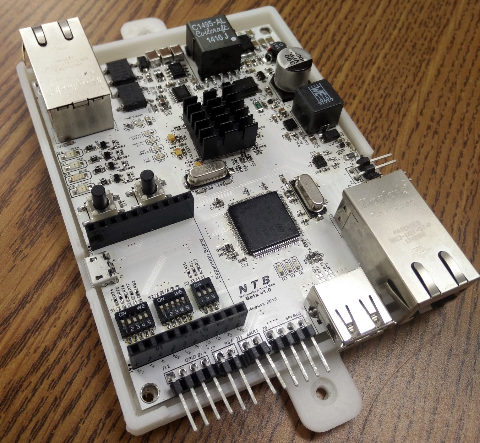
Figure 3: Custom anchor with ARM Cortex M4 processor and UWB slot.

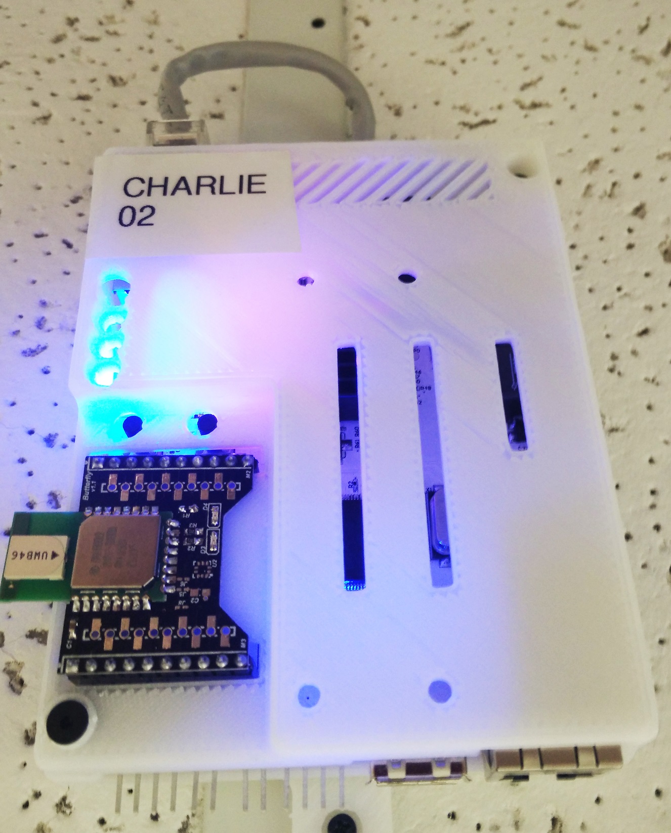
Figure 4: Ceiling-mounted anchor with UWB radio in 3D-printed enclosure.

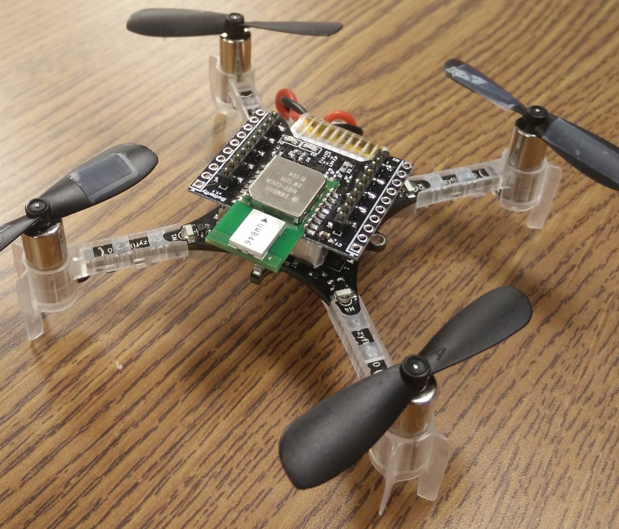
Figure 5: CrazyFlie 2.0 quadrotor helicopter with UWB expansion.

VI-B Experimental Setup

We evaluate the performance of Algorithm $1$ on a custom ultra-wideband (UWB) RF testbed based on the DecaWave DW1000 IR-UWB radio. The overall setup is presented in Figure 2. The main components of the considered testbed can be summarized as follows:

• The motion capture system with eight cameras capable of performing 3D rigid body position measurement with a accuracy of less than $0.5$ mm accuracy. The presented results consider the motion capture estimates as the true position, even though we qualify here that all results are accurate with respect to the motion capture accuracy.

• Fixed nodes consist of custom-built circuit boards equipped with ARM Cortex M4 processors of $196$ MHz powered over Ethernet and communicating by Decawave DW1000 ultra-wideband radios, as shown in Figures 5 and 5. Each anchor performs the single and double-sided two-way range measurement with its neighbors. The used Decawave radio is equipped with a temperature-compensated crystal oscillator with frequency of $38.4$ MHz and stated frequency stability of $\pm 2$ ppm. We installed eight UWB anchor nodes in different positions in a $10\times 9$ $m^{2}$ laboratory. More specifically, six anchors are placed on the ceiling at about $2.5$ m hight, and the other two are spotted at the waist height of about $1$ m to disambiguate positions on the vertical axis in a better manner.

• The battery-powered mobile node is a modified CrazyFlie 2.0 helicopter is equipped with the same DW1000 radio and ARM Cortex M4 processor, as shown in Figure 5.

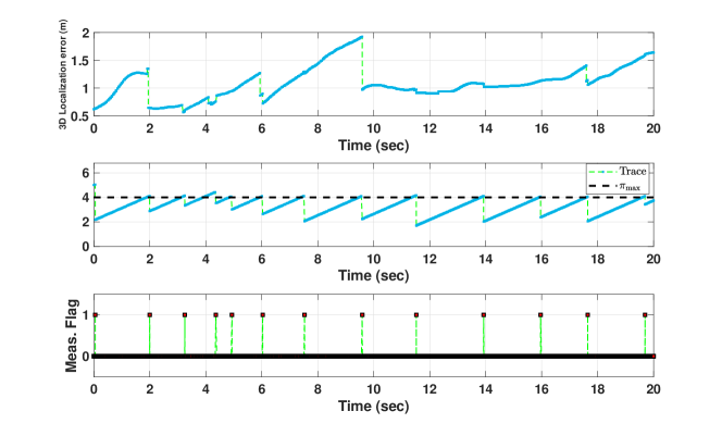
Figure 6: Snapshot of $20$ seconds of the conducted experiments. The threshold is set to $4$ $m^{2}$. The 3D localization error and trace value $\operatorname{\mathsf{tr}}(WP_{L,i|i}W^{*})$ are shown in the first and second sub-figures, respectively. The measurement and diffusion flags are the same and shown in the third sub-figure in which a value of $1$ indicates of the step execution, while $0$ means skipping the step at the corresponding time instance. Time update step is executed all the time.

VI-C Experiments

In the conducted experiments, we mainly consider the communication overhead and the associated accuracy on different network topologies to demonstrate the effectiveness of the proposed algorithm. We aim to apply the triggering logic based on the expected estimation error of the mobile node location. The mobile node is chosen as a leader and its diffusion error covariance matrix is $P_{L,i|i}$ in Algorithm 1.

To give the intuition behind evaluation of the proposed algorithm, we present the results of running a portion of the experiments in Figure 6. The mobile node flies at different speeds in the testing laboratory while seeking to save computational and communication resources. The threshold $\pi_{\max}$ is set to $4$ $m^{2}$. The second graph in Figure 6 presents the behavior of $\operatorname{\mathsf{tr}}(WP_{L,i|i}W^{T})$. All nodes execute the time update step when $\operatorname{\mathsf{tr}}(WP_{L,i|i}W^{T})$ is less than $\pi_{\max}$. Consequently, we decrease the spending in terms of measurements, message exchange, and computational costs. The effect on the estimated localization error of the mobile node can be clearly seen in the first graph of Figure 6. As soon as $\operatorname{\mathsf{tr}}(WP_{L,i|i}W^{T})$ reaches the threshold $\pi_{\max}$, all nodes are triggered to start measuring and to exchange messages to decrease $\operatorname{\mathsf{tr}}(WP_{L,i|i}W^{T})$ back to the allowed range. The third graph in Figure 6 demonstrates the case when the measurement update step is executed at all nodes. For instance, we can see that the measurement update step happens at the time instances $0.1,2.7,4.4,5.1,7.0,10.1,12.9,$ and $16.4,$ so that we can notice the decrease in the localization error in the first graph at the same time instances. Similarly, the diffusion update step is executed just after the measurement update step. The time update step is executed all the time.

The CrazyFlie flied across the laboratory over four different sessions. Each session was conducted on a different day with a different number of students in the room. The path of the CrazyFlie was a random walk for each session. We repeated the experiments while setting a different threshold, then calculated the number of shared messages between nodes and the localization error reported by the motion capture system.

VI-C1 Case Study on a Fully-Connected Network

We illustrate the effectiveness of the proposed triggering algorithm by outlining the amount of saving on the communication overhead and the associated localization error by applying the algorithm over a fully-connected network.

Communication Analysis

Figure 7(a) shows the effect of changing the threshold value $\pi_{\max}$ on the percentage of the saved message for a fully-connected network. The zero threshold refers to the case of sending all messages ($1,975,632$ messages in total) and running the three steps of the algorithm in the normal mode. Setting the threshold to $1$ $m^{2}$ allows saving approximately $86.2\%$ of the overall number of messages. Moreover, the threshold of $5$ $m^{2}$ leads to saving $98\%$ of the total number of messages.

Accuracy Analysis

We have conducted a study to identify what is the tradeoff between the 3D-localization errors corresponding to each threshold value $\pi_{\max}$. The error plot in Figure 7(c) summarizes the obtained results of this case study. The red rectangles correspond to the mean values of the localization error, while the vertical lines represent the standard deviation around that mean value. At threshold $\pi_{\max}=0$, we do not save any resources, and we achieve $0.377$ $m$ mean localization error with the standard deviation of $0.195$ $m$. While, $\pi_{\max}=5$ $m^{2}$ results in a $1.155$ $m$ mean error with the standard deviation of $0.71$ $m$. Finally, $\pi_{\max}=10$ $m^{2}$ allows achieving the mean error of $1.923$ $m$ with the standard deviation of $0.790$ $m$. The appropriate thresholds can be set by users based on their needs.

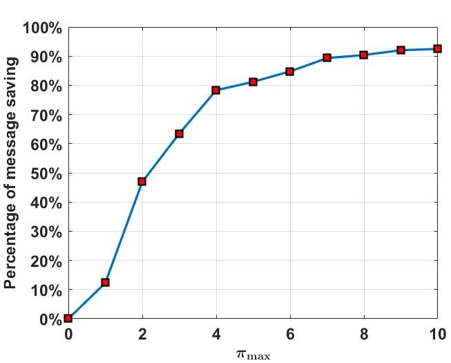
(a) Effect of changing the threshold value $\pi_{\max}$ on the percentage of the saved messages for a fully connected network.	(b) Effect of changing the threshold value $\pi_{\max}$ on the percentage of the saved messages for a partially connected network.
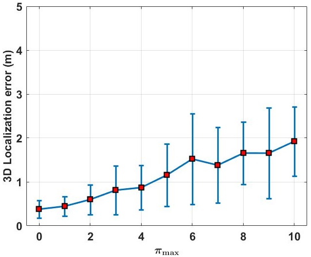
(c) Effect of changing the threshold value $\pi_{\max}$ on the 3D localization error of the CrazyFlie for a fully connected network.	(d) Effect of changing the threshold value $\pi_{\max}$ on the 3D localization error of the CrazyFlie for a partially connected network.

Figure 7: Effect of changing the threshold value $\pi_{\max}$ on a fully connected network and partially connected one.

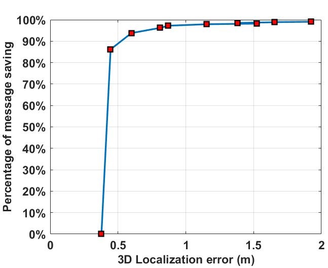
Figure 8: The tradeoff between the communication overhead saving and the mean 3D localization error of the CrazyFlie.

The proposed algorithm is used to restrict the amount of processing, sensing, and communication. This restriction allows reducing dramatically the communication overhead in the network, however it may potentially lead to deterioration of network performance. We analyze the tradeoff between the number of messages sent in the wireless network and performance of estimation algorithm. Figure 8 shows the tradeoff between the communication overhead and the mean 3D localization error. Notably, saving $86.2\%$ of the communication overhead leads to the increase in the localization error by $16.57\%$. This was calculated by considering the mean localization error plus the standard deviation at thresholds $0$ and $1$.

VI-C2 Case Study on a Partially Connected Network

We considered another case study in which every node among the nine considered ones is connected to only four neighbors instead of eight neighbors in the previous case study. We analyze the communication saving and the associated localization error. Figure 7(b) summarizes the observed results. It should be noted that setting the threshold to $5$ leads to saving approximately $81.2\%$ of the overall number of messages. Moreover, the threshold of $\pi_{\max}=9$ $m^{2}$ allows saving $92\%$ of the total number of messages. The error plot in Figure 7(d) summarizes the obtained results of this case study. Here, the red rectangles correspond to the mean values of the localization error, while the vertical lines represent the standard deviation around that mean value. At threshold $\pi_{\max}=0$ $m^{2}$, we do not save any resources, and we can achieve $2$ $m$ mean localization error with standard deviation of $0.6$ $m$ in the case when the network is partially connected, as described before. While $\pi_{\max}=5$ $m^{2}$ results in the mean error of $2.6$ $m$ with the standard deviation of $0.49$ $m$.

VII Conclusion

In the present study, we investigated the energy-aware aspect of the distributed estimation problem with regard to the multi-sensor system with event-triggered processing schedules. More specifically, we proposed an unbiased event-triggered distributed diffusion Kalman filter for wireless networks based on the diffusion covariance matrix. We tested the proposed algorithm on the distributed localization and time synchronization application. Several experiments were conducted using the real custom ultra-wideband wireless anchor nodes and mobile quadrotor. The obtained results indicate that the proposed algorithm is has robust performance, and is efficient in terms of using computational and communication resources.

References

- [1] J. Yick, B. Mukherjee, and D. Ghosal, “Wireless sensor network survey,” Computer networks, vol. 52, no. 12, pp. 2292–2330, 2008.
- [2] A. J. Goldsmith and S. B. Wicker, “Design challenges for energy-constrained ad hoc wireless networks,” IEEE wireless communications, vol. 9, no. 4, pp. 8–27, 2002.
- [3] G. J. Pottie and W. J. Kaiser, “Wireless integrated network sensors,” Communications of the ACM, vol. 43, no. 5, pp. 51–58, 2000.
- [4] K. Kumar, J. Liu, Y.-H. Lu, and B. Bhargava, “A survey of computation offloading for mobile systems,” Mobile Networks and Applications, vol. 18, no. 1, pp. 129–140, 2013.
- [5] W. R. Heinzelman, A. Chandrakasan, and H. Balakrishnan, “Energy-efficient communication protocol for wireless microsensor networks,” in Proc. of the 33rd Annual Hawaii International Conference on System Sciences, vol. 2, 2000, pp. 1–10.
- [6] R. Olfati-Saber, “Distributed Kalman filtering for sensor networks,” in 46th IEEE Conference on Decision and Control, Dec 2007, pp. 5492–5498.
- [7] F. S. Cattivelli, C. G. Lopes, and A. H. Sayed, “Diffusion strategies for distributed Kalman filtering: formulation and performance analysis,” Proc. Cognitive Information Processing, pp. 36–41, 2008.
- [8] A. Alanwar, H. Ferraz, K. Hsieh, R. Thazhath, P. Martin, J. Hespanha, and M. Srivastava, “D-SLATS: Distributed simultaneous localization and time synchronization,” in Proc. of the 18th ACM International Symposium on Mobile Ad Hoc Networking and Computing, 2017, pp. 1–10. [Online]. Available: https://doi.org/10.1145/3084041.3084049
- [9] H. Ferraz, A. Alanwar, M. Srivastava, and J. P. Hespanha, “Node localization based on distributed constrained optimization using Jacobi’s method,” in 2017 IEEE 56th Annual Conference on Decision and Control, Dec 2017, pp. 3380–3385.
- [10] L. Xiao, S. Boyd, and S. Lall, “A space-time diffusion scheme for peer-to-peer least-squares estimation,” in Proc. of the 5th international conference on Information Processing in Sensor Networks. ACM, 2006, pp. 168–176.
- [11] I. D. Schizas, G. B. Giannakis, S. I. Roumeliotis, and A. Ribeiro, “Consensus in ad hoc WSNs with noisy links—part ii: Distributed estimation and smoothing of random signals,” IEEE Transactions on Signal Processing, vol. 56, no. 4, pp. 1650–1666, 2008.
- [12] U. A. Khan and J. M. Moura, “Distributing the Kalman filter for large-scale systems,” IEEE Transactions on Signal Processing, vol. 56, no. 10, pp. 4919–4935, 2008.
- [13] R. Grone, C. R. Johnson, E. M. Sá, and H. Wolkowicz, “Positive definite completions of partial hermitian matrices,” Linear algebra and its applications, vol. 58, pp. 109–124, 1984.
- [14] Y. S. Suh, V. H. Nguyen, and Y. S. Ro, “Modified Kalman filter for networked monitoring systems employing a send-on-delta method,” Automatica, vol. 43, no. 2, pp. 332 – 338, 2007.
- [15] J. Wu, Q.-S. Jia, K. H. Johansson, and L. Shi, “Event-based sensor data scheduling: Trade-off between communication rate and estimation quality,” IEEE Transactions on Automatic Control, vol. 58, no. 4, pp. 1041–1046, 2013.
- [16] S. Trimpe and R. D’Andrea, “Event-based state estimation with variance-based triggering,” IEEE Transactions on Automatic Control, vol. 59, no. 12, pp. 3266–3281, 2014.
- [17] D. Shi, T. Chen, and L. Shi, “On set-valued Kalman filtering and its application to event-based state estimation,” IEEE Transactions on Automatic Control, vol. 60, no. 5, pp. 1275–1290, 2015.
- [18] D. Han, Y. Mo, J. Wu, S. Weerakkody, B. Sinopoli, and L. Shi, “Stochastic event-triggered sensor schedule for remote state estimation,” IEEE Transactions on Automatic Control, vol. 60, no. 10, pp. 2661–2675, 2015.
- [19] L. Li, M. Lemmon, and X. Wang, “Event-triggered state estimation in vector linear processes,” in American Control Conference. IEEE, 2010, pp. 2138–2143.
- [20] L. Li, Z. Wang, and M. Lemmon, “Polynomial approximation of optimal event triggers for state estimation problems using sostools,” in American Control Conference. IEEE, 2013, pp. 2699–2704.
- [21] L. Groff, L. Moreira, J. G. da Silva, and D. Sbarbaro, “Observer-based event-triggered control: A discrete-time approach,” in American Control Conference. IEEE, 2016, pp. 4245–4250.
- [22] D. N. Borgers and W. M. Heemels, “Event-separation properties of event-triggered control systems,” IEEE Transactions on Automatic Control, vol. 59, no. 10, pp. 2644–2656, 2014.
- [23] D. Shi, L. Shi, and T. Chen, “Linear gaussian systems and event-based state estimation,” in Event-Based State Estimation. Springer, 2016, pp. 33–46.
- [24] A. Molin, H. Sandberg, and K. H. Johansson, “Consistency-preserving event-triggered estimation in sensor networks,” in Conference on Decision and Control. IEEE, 2015, pp. 7494–7501.
- [25] G. Battistelli, L. Chisci, and D. Selvi, “Distributed Kalman filtering with data-driven communication,” in 19th International Conference on Information Fusion. IEEE, 2016, pp. 1042–1048.
- [26] H. Yan, P. Li, H. Zhang, X. Zhan, and F. Yang, “Event-triggered distributed fusion estimation of networked multisensor systems with limited information,” IEEE Transactions on Systems, Man, and Cybernetics: Systems, pp. 1–8, 2018.
- [27] G. Battistelli, L. Chisci, and D. Selvi, “A distributed Kalman filter with event-triggered communication and guaranteed stability,” Automatica, vol. 93, pp. 75 – 82, 2018.
- [28] X. He, C. Hu, Y. Hong, L. Shi, and H. Fang, “Distributed kalman filters with state equality constraints: Time-based and event-triggered communications,” IEEE Transactions on Automatic Control, vol. 65, no. 1, pp. 28–43, Jan 2020.
- [29] X. He, C. Hu, W. Xue, and H. Fang, “On event-based distributed kalman filter with information matrix triggers,” IFAC-PapersOnLine, vol. 50, no. 1, pp. 14 308–14 313, 2017.
- [30] W. Li, Y. Jia, and J. Du, “Event-triggered Kalman consensus filter over sensor networks,” IET Control Theory & Applications, vol. 10, no. 1, pp. 103–110, 2016.
- [31] C. Zhang and Y. Jia, “Distributed Kalman consensus filter with event-triggered communication: Formulation and stability analysis,” Journal of the Franklin Institute, vol. 354, no. 13, pp. 5486–5502, 2017.
- [32] X. Wang and M. D. Lemmon, “Event-triggering in distributed networked control systems,” IEEE Transactions on Automatic Control, vol. 56, no. 3, pp. 586–601, 2010.
- [33] S. Trimpe, “Distributed event-based state estimation,” arXiv preprint arXiv:1511.05223, 2015.
- [34] L. Zou, Z.-D. Wang, and D.-H. Zhou, “Event-based control and filtering of networked systems: A survey,” International Journal of Automation and Computing, pp. 1–15, 2017.
- [35] V. Vahidpour, A. Rastegarnia, A. Khalili, W. Bazzi, and S. Sanei, “Partial diffusion Kalman filtering,” arXiv preprint arXiv:1705.08920, 2017.
- [36] Y. Chen, G. Qi, Y. Li, and A. Sheng, “Diffusion Kalman filtering with multi-channel decoupled event-triggered strategy and its application to the optic-electric sensor network,” Information Fusion, vol. 36, pp. 233–242, 2017.
- [37] A. H. Sayed, Fundamentals of adaptive filtering. John Wiley & Sons, 2003.
- [38] F. S. Cattivelli and A. H. Sayed, “Diffusion strategies for distributed Kalman filtering and smoothing,” IEEE Transactions on Automatic Control, vol. 55, no. 9, pp. 2069–2084, 2010.