Inflation in Random Landscapes
with two energy scales

Abstract

We investigate inflation in a multi-dimensional landscape with a hierarchy of energy scales, motivated by the string theory, where the energy scale of Kahler moduli is usually assumed to be much lower than that of complex structure moduli and dilaton field. We argue that in such a landscape, the dynamics of slow-roll inflation is governed by the low-energy potential, while the initial condition for inflation are determined by tunneling through high-energy barriers. We then use the scale factor cutoff measure to calculate the probability distribution for the number of inflationary e-folds and the amplitude of density fluctuations $Q$, assuming that the low-energy landscape is described by a random Gaussian potential with a correlation length much smaller than $M_{\rm pl}$. We find that the distribution for $Q$ has a unique shape and a preferred domain, which depends on the parameters of the low-energy landscape. We discuss some observational implications of this distribution and the constraints it imposes on the landscape parameters.

1 Introduction

String theory is currently our best candidate for a fundamental theory of nature, but its internal consistency requires it to live on a higher dimensional spacetime. This forces us to think of a mechanism of compactification that allows the theory to be compatible with low energy observations. The effective four dimensional theory that results from this compactification process is then endowed with a large number of fields that parametrize the geometric properties of the internal space. We therefore expect a large number of metastable vacua of the compactification potential where these four dimensional fields would be stabilized.

Models of flux compatification, where fluxes are wrapped around the internal cycles of the compact manifold, have been extensively studied in the literature [1]. This type of scenarios leads to an incredibly large ensemble of vacua, due to the huge numbers of combinatoric possibilities [2].

In order to explore the implications of the String Theory Landscape in cosmology, one needs to understand the basic properties of the compactification potential. Due to its intrinsic complexity and the large number of fields involved, it seems reasonable to use statistical techniques. Following these ideas it has been recently suggested (see, e.g., [3, 4, 5, 6, 7, 8, 9, 10, 11, 12, 13, 14, 15] ) that one could model the Landscape potential as a Gaussian Random Field (GRF) on the space of the low energy scalar fields, the moduli. This is a simple model designed to capture the random behavior of a low-energy potential that has a large number of contributions of different physical origin.

Alternatively, one could take the opposite approach where one investigates a particular set of potential realizations that appear in the low energy description of a specific compactification scenario. This approach has also been pursued in the literature for a small number of moduli fields in [22, 23, 24].

This kind of top-down approach, where one identifies a concrete mechanisms that should be invoked to stabilize the moduli, highlights the fact that not all the moduli should be treated in the same way. In fact, it is pretty clear that all the models of compactification so far used in the literature work by introducing several ingredients that stabilize some sectors of the moduli space but not others. This leads to the possibility of a hierarchy of scales in the compactification process. One can take, for example, models of Type IIB compactification to realize that the mechanisms that stabilize the complex structure moduli and the dilaton are very different in nature than the one that fixes the Kahler moduli, leading to a hierachy of masses [25, 26, 23].

Following these considerations, in the present paper we investigate a Random Gaussian Landscape with a hierarchy of two different scales: a high-energy and low-energy sectors of the Landscape. We will show that this structure of the Landscape has important cosmological implications. In particular, we will argue that transitions by bubble nucleation between the vacua in the low-energy landscape are likely to be subdominant. This implies that the initial conditions for slow-roll inflation, which occurs after tunneling from a false vacuum to a slow-roll region, are likely to be determined by tunneling through the barriers of the high-energy landscape. However, after the bubble nucleation, the dynamics of slow-roll inflation is governed by the low-energy landscape.

Thus, in a two-scale landscape, bubble nucleation and slow-roll inflation occur at different energy scales. We use this fact to calculate the probability distribution for the maximal number of e-folds, $N_{\rm max}$, and the amplitude of density fluctuations $Q$ in the multiverse. We show that the probability function of $Q$ has a unique form and a preferred domain depending on parameters of the low energy landscape.

This paper is organized as follows. In the next section we specify the model of a two-scale landscape and argue (i) that tunnelings in the low-energy sector can be neglected and (ii) that the tunneling points that determine the initial conditions in the bubbles are randomly distributed in the low-energy landscape. We then review some relevant features of slow-roll inflation. In Sec. 3, we calculate the prior probability distribution for the number of inflationary e-foldings and the amplitude of density fluctuations in a one-dimensional landscape. (Here the word ”prior” means ”disregarding anthropic considerations”.) In Sec. 4, we extend this calculation to a multi-dimensional landscape and show that the resulting distribution is essentially the same as in one dimension. The anthropic factor and some observational implications of our results are discussed in Sec. 5. Finally, our conclusions are summarized and discussed in Sec. 6. We use the reduced Planck units ($M_{\rm pl}\simeq 2.4\times 10^{18}\ {\rm GeV}\equiv 1$) throughout the paper.

2 A two-scale Landscape

We consider a model with two types of fields denoted as $\phi_{i}$ ($i=1,2,\dots,D_{\rm L}$) and $\psi_{j}$ ($j=1,2,\dots,D_{\rm H}$) that represent different sectors of the moduli space. In particular, one could think of $\phi_{i}$ as the Kahler moduli sector and $\psi_{j}$ as the complex structure moduli and the dilaton of a type IIB compactification.

We assume that the potential $U({\bm{\phi}},{\bm{\psi}})$ has two characteristic energy scales $U_{\rm L}$ and $U_{\rm H}$ and two correlation lengths $\Lambda_{\rm L}$ and $\Lambda_{\rm H}$ in the field space, where the correlation function of the potential $F(|\bm{\phi}_{1}-\bm{\phi}_{2}|,|\bm{\psi}_{1}-\bm{\psi}_{2}|)$ rapidly decays at $|\bm{\phi}_{1}-\bm{\phi}_{2}|\gg\Lambda_{\rm L}$ or $|\bm{\psi}_{1}-\bm{\psi}_{2}|\gg\Lambda_{\rm H}$. We assume also that the potential changes by $\sim U_{\rm L}$ when the field value changes by $\Delta\bm{\phi}\sim\Lambda_{\rm L}$, while it changes by $\sim U_{\rm H}$ when $\Delta\bm{\psi}\sim\Lambda_{\rm H}$. We consider the case where $U_{\rm L}\ll U_{\rm H}$ and $\Lambda_{\rm L},\Lambda_{\rm H}\ll 1$. We shall also assume that the two correlation lengths are not much different from one another,

$$\Lambda_{L}\sim\Lambda_{H}.$$ (1)

According to the effective theory perspective, we expect that the potential of scalar fields is well described by a Taylor expansion in the neighborhood of any point in the field space. Since the potential is characterized by $U_{a}$ and $\Lambda_{a}$ ($a={\rm L},{\rm H}$), we expect that the typical values of Taylor coefficients are given by

$$\frac{\partial^{n}U}{\partial\phi_{i}^{n}}\sim\frac{U_{\rm L}}{\Lambda_{\rm L}^{n}}\qquad\frac{\partial^{n}U}{\partial\psi_{i}^{n}}\sim\frac{U_{\rm H}}{\Lambda_{\rm H}^{n}},\qquad\frac{\partial^{m+n}U}{\partial\phi_{i}^{m}\partial\psi_{j}^{n}}\sim\frac{U_{\rm L}}{\Lambda_{\rm L}^{m}\Lambda_{\rm H}^{n}},$$ (2)

at a generic point in the landscape. The probability distribution of Taylor coefficients can be derived once we specify the correlation function $F(|\bm{\phi}_{1}-\bm{\phi}_{2}|,|{\bm{\psi}}_{1}-{\bm{\psi}}_{2}|)$.

Here we explicitly write an example of such a correlation function. Let us first decompose the potential into two terms plus a constant term $\bar{U}_{T}$

$$U({\bm{\phi}},{\bm{\psi}})=U_{\rm H}({\bm{\psi}})+U_{\rm L}({\bm{\phi}},{\bm{\psi}})+\bar{U}_{T}.$$ (3)

Then, in order to satisfy the properties mentioned earlier we can take the functions $U_{\rm H}({\bm{\psi}})$ and $U_{\rm L}({\bm{\phi}},{\bm{\psi}})$ as Gaussian Random Fields with the following properties

$$\left<U_{\rm H}({\bm{\psi}})\right>=\left<U_{\rm L}({\bm{\phi}},{\bm{\psi}})\right>=0$$ (4)

$$\left<U_{\rm H}({\bm{\psi}}_{1})U_{\rm H}({\bm{\psi}}_{2})\right>=U_{\rm H}^{2}F_{\rm H}\left(\frac{\Delta\psi}{\Lambda_{\rm H}}\right)$$

$$\left<U_{\rm L}({\bm{\phi}}_{1},{\bm{\psi}}_{1})U_{\rm L}({\bm{\phi}}_{2},{\bm{\psi}}_{2})\right>=U_{\rm L}^{2}F_{\rm L}\left(\frac{\Delta\phi}{\Lambda_{\rm L}},\frac{\Delta\psi}{\Lambda_{\rm H}}\right)$$

$$\left<U_{\rm H}({\bm{\psi}}_{1})U_{\rm L}({\bm{\phi}}_{2},{\bm{\psi}}_{2})\right>=0,$$ (5)

where $\Delta\psi\equiv|{\bm{\psi}}_{1}-{\bm{\psi}}_{2}|$ and $\Delta\phi\equiv|{\bm{\phi}}_{1}-{\bm{\phi}}_{2}|$. The functions $F_{\rm H}(x)$ and $F_{\rm L}(x,y)$ decay rapidly at $x\gg 1$ and/or $y\gg 1$. The correlators are often chosen in the form $F_{\rm H}(x)\propto\exp(-x^{2}/2)$ and $F_{\rm L}(x,y)\propto\exp(-x^{2}/2-y^{2}/2)$. However, this is a very special case, in which the statistics of the potential minima is rather different from that for a generic correlator. In particular, the minima are much stronger localized in energy in the limit of large $D$ [27]. In this paper we focus on the generic case, as it was done in Ref. [14].

The minima of the Gaussian random field $U_{\rm H}({\bm{\psi}})$ centered around zero and a characteristic scale of $U_{\rm H}$ like the one we use here for the high-energy sector of our Landscape are localized at $U\sim-\sqrt{D_{\rm H}}U_{\rm H}$ within a range of $\Delta U\sim U_{\rm H}$ [27]. We shall therefore assume that the constant term $\bar{U}_{T}$ is of the order $\sqrt{D_{\rm H}}U_{\rm H}$, so that we do not have to worry that almost all minima of $U({\bm{\phi}},{\bm{\psi}})$ are at $U<0$. Alternatively, one might add a term like $m^{2}{\bm{\psi}}^{2}$ with $m^{2}\ll U_{\rm H}/\Lambda_{\rm H}^{2}$, instead of a constant $\bar{U}_{T}$, so that $\left<U({\bm{\phi}},{\bm{\psi}})\right>$ can be as large as $\sqrt{D_{\rm H}}U_{\rm H}$ somewhere in the landscape. Such a term could arise due to mixing between axions and flux fields [28, 29].

Random potentials specified by the correlators (4) and (5) reflect the hierarchy between different sectors in the String Theory Landscape, although it is likely that the specific forms of the potentials that can be computed will not fall under this simple statistical description. On the other hand, we believe that our results should have a wider applicability than the model (4) and (5). The key assumption that we are going to adopt is that the low-energy potential $U_{\rm L}({\bm{\phi}},{\bm{\psi}})$ at a fixed $\psi$ is a random Gaussian field. However, our conclusions are rather insensitive to the assumptions we make about the high-energy landscape $U_{\rm H}({\bm{\psi}})$, as long as a few basic conditions are satisfied. These conditions are listed in section 6 and are likely to hold in a wide class of models.

Of course the Gaussian nature of the low-energy potential is a strong assumption (see for example [23, 30, 31]), so such models should be regarded only as toy models for the string theory landscape. A realistic landscape is likely to include some runaway directions in which some of the compact dimensions decompactify [32] (see also, e.g., Ref. [33]). Such runaway potentials do not occur in a random Gaussian field. Moreover, destabilization of the volume modulus, resulting in a complete decompactification, should lead to a state with $U=0$, which is inconsistent with the separation into high and low-energy sectors (since most of the vacua in the landscape have $U\sim U_{H}$). On the other hand, it may be an adequate approximation to focus on the central region of the moduli space containing stable vacua. The energy scale of Kahler moduli in that region may be much smaller than that of complex structure moduli, since the stabilization mechanisms are different for these fields. Our two-scale model may thus be a useful toy model for the relevant part of the landscape, which includes metastable vacua (and excludes the unstable runaway configurations). It would be interesting to investigate the issues discussed in this paper in a more realistic setup where ensembles of potentials can be obtained.

2.1 Tunneling transitions

In the cosmological context, each positive-energy vacuum becomes a site of eternal inflation, and transitions between different vacua constantly occur via bubble nucleation, resulting in a multiverse of bubbles with diverse properties. The initial conditions in each bubble are determined by the instanton describing nucleation of that bubble from its parent vacuum. The aim of this paper is to calculate the probability distribution for some observables in this multiverse.

Slow-roll inflation must have occurred in our region after the tunneling event that led to the formation of our bubble. Since we cannot observe anything prior to the tunneling, all observables can be calculated once we specify the tunneling endpoint in the landscape (which is also the initial point of the slow-roll inflation).

Observational predictions in multiverse models depend on one’s choice of the probability measure. Different measure prescriptions can give vastly different answers. (For a review of this “measure problem” see, e.g., [34].) However, measures that are free from obvious pathologies, such as the scale factor [35, 36, 37, 38], lightcone [38] and watcher [39, 40] measures, tend to make similar predictions. For definiteness we shall use the scale-factor cutoff measure. The probability of observing a certain kind of region is then proportional to the average number of observers in such regions under the cutoff surface of a constant scale factor $a$ in the limit of $a\to\infty$.

Let us label the vacua in the landscape by an index $i$. The probability of observing a bubble of type $i$ nucleated in a false vacuum $j$ can then be roughly estimated as (see, e.g., Ref. [41])

$$P_{ij}\propto n_{ij}^{(\rm obs)}\kappa_{ij}s_{j}\leavevmode\nobreak\ ,$$ (6)

where $n_{ij}^{(\rm obs)}$ is the number of observers per unit mass in this type of bubble. We focus on bubbles having the same low-energy microphysics as ours, described by the Standard Model. Then $n_{ij}^{(\rm obs)}$ depends on $Q$, on the present cosmological constant $\rho_{v}$, and on the curvature parameter $\Omega_{c}$, which is determined by the number of e-folds of slow-roll inflation.

$\kappa_{ij}$ in Eq. (6) is the transition rate from $j$ to $i$ per Hubble volume per Hubble time, and $s_{j}$ is the fraction of inflating volume in parent vacuum $j$ on a constant scale factor slice. $s_{j}$ is proportional to the $j$-th component of the eigenvector of the following matrix with the largest eigenvalue [42, 43]:

$$M_{ij}=\kappa_{ij}-\delta_{ij}\sum_{r}\kappa_{ri}\leavevmode\nobreak\ .$$ (7)

Since there are two energy scales in the landscape, there are two types of vacuum transitions, corresponding to tunnelings through high- and low-energy barriers. The corresponding transition rates can be vastly different. They can be estimated as $\kappa_{ij}\propto\exp(-S_{ij})$, where $S_{ij}$ is the instanton action and can be written as

$$S_{ij}=\frac{\Lambda_{a}^{4}}{U_{a}}{\bar{S}}_{ij}\leavevmode\nobreak\ ,$$ (8)

by a rescale of variables. Here, $a={\rm L}$ or ${\rm H}$ and ${\bar{S}}_{ij}$ is independent of $U_{a}$ and $\Lambda_{a}$. In a one-dimensional Gaussian landscape, the rescaled action ${\bar{S}}_{ij}$ typically takes values between $\sim 10$ and $\sim 10^{4}$ [13]. One can expect a similar range for ${\bar{S}}_{ij}$ in a higher-dimensional landscape.

With $U_{H}\gg U_{L}$ and $\Lambda_{H}\sim\Lambda_{L}$, Eq. (8) tells us that vacuum transitions in the low-energy sector are very strongly suppressed. The probability of observing anthropic bubbles resulting from such transitions is then negligibly small; hence we shall concentrate on bubbles produced by tunnelings through high-energy barriers.

To a good approximation, an instanton describing such a tunneling can be found by solving the Euclidean equations of motion for the fields ${\bm{\psi}}$ in the potential $U_{H}({\bm{\psi}})$, disregarding their interaction with the low-energy fields ${\bm{\phi}}$. The typical size of the instanton (i.e., the initial bubble radius) is then

$$r_{0}\sim\frac{\Lambda_{\rm H}}{\sqrt{U_{\rm H}}}.$$ (9)

The tunneling endpoint is typically very close to a local minimum of $U_{\rm H}({\bm{\psi}})$ for a generic potential [44], but we do not assume this in the following analysis.

We next consider the Euclidean equations of motion for the ${\bm{\phi}}$ fields,

$$\frac{{d}^{2}\phi_{i}}{{d}r^{2}}+\frac{3}{r}\frac{{d}\phi_{i}}{{d}r}-\frac{\partial U_{\rm L}}{\partial\phi_{i}}=0\leavevmode\nobreak\ .$$ (10)

The displacement of ${\bm{\phi}}$ due to the tunneling process can be estimated as

$$\Delta{\bm{\phi}} \sim \frac{U_{\rm L}}{\Lambda_{\rm L}}r_{0}^{2}$$ (11)

$$\sim \Lambda_{\rm L}\frac{\Lambda_{\rm H}^{2}}{\Lambda_{\rm L}^{2}}\frac{U_{\rm L}}{U_{\rm H}}\ll\Lambda_{L},$$ (12)

where we have used $\partial U_{\rm L}/\partial\phi_{i}\sim U_{\rm L}/\Lambda_{\rm L}$ and Eqs. (1) and (9). This indicates that the low-energy fields ${\bm{\phi}}$ remain largely unperturbed during a high-energy tunneling.

To check this qualitative argument, we consider the following toy model with only two fields, $\phi$ and $\psi$:

$$U(\phi,\psi)=U_{\rm H}\left[\frac{c_{2}}{2}\gamma\left(\frac{\phi}{\Lambda_{\rm L}}\right)^{2}+\frac{c_{3}}{6}\gamma\left(\frac{\phi}{\Lambda_{\rm L}}\right)^{3}+\frac{c_{\psi}}{2}\left(\frac{\psi}{\Lambda_{\rm H}}\right)^{2}\right]\times$$

$$\leavevmode\nobreak\ \leavevmode\nobreak\ \leavevmode\nobreak\ \leavevmode\nobreak\ \leavevmode\nobreak\ \leavevmode\nobreak\ \leavevmode\nobreak\ \leavevmode\nobreak\ \leavevmode\nobreak\ \leavevmode\nobreak\ \leavevmode\nobreak\ \leavevmode\nobreak\ \leavevmode\nobreak\ \leavevmode\nobreak\ \times\left[\frac{c_{\phi f}}{2}\gamma\left(\frac{\phi}{\Lambda_{\rm L}}-R\cos\theta\right)^{2}+\frac{c_{\psi f}}{2}\left(\frac{\psi}{\Lambda_{\rm H}}-R\sin\theta\right)^{2}+c_{h}\right]$$ (13)

where $\gamma\equiv U_{\rm L}/U_{\rm H}\ll 1$. The parameters $c_{2}$, $c_{3}$, $c_{\psi}$, $c_{1f}$, $c_{2f}$, $R$, $\theta$, $c_{h}$ are assumed to be $O(1)$; we take $c_{i}=1$ ($i=3,\psi,\phi f,\psi f$), $c_{2}=0$, $c_{h}=0.5$ and $R=5$ as an example. The parameters $R$ and $\theta$ determine the location of the false vacuum, and $c_{h}$ determines its energy density. An example of this potential with $\theta=2\pi/5$, $\Lambda_{L}=\Lambda_{H}$ and $\gamma=U_{\rm L}/U_{\rm H}=0.02$ is shown in Fig. 1, where the false vacuum is marked by a blue dot. We also show in Fig. 1 an inflection point with a white dot. In the following section we will consider this kind of region as one of the forms of the potential to be responsible for the inflationary period after the tunneling event.

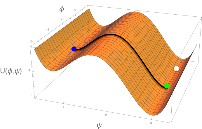
Figure 1: An example of the potential (13), where we use the parameters indicated in the text. The false vacuum is marked by a blue dot. The black line shows the instanton trajectory, and the green dot is the tunneling point. We also show an inflection point with a white dot.

We used the public code developed in Ref. [45] to solve the Euclidean equations of motion and determine the tunneling (end)point $(\phi,\psi)=(\phi_{0},\psi_{0})$ corresponding to bubble nucleation. We assume that gravitational effects on the tunneling can be neglected, which is usually the case for $\Lambda_{a}\ll 1$. The instanton trajectory is shown as a black line in the figure, with the tunneling point indicated by a green dot.

To illustrate the dependence of the tunneling point on $\gamma\equiv U_{\rm L}/U_{\rm H}$, we plot $\left|\phi_{0}-\phi_{\rm FV}\right|/|\phi_{\rm FV}|$ as a function of $\gamma$ in Fig. 2, where $\phi_{\rm FV}$ is the field value at the false vacuum. We see that for $\gamma\ll 1$ the field $\phi$ changes very little due to the tunneling process, as expected.

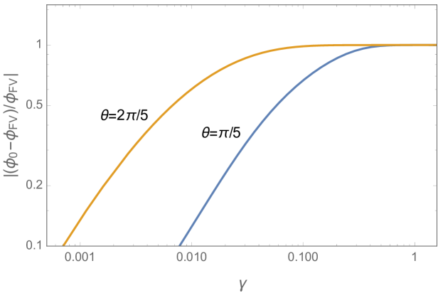
Figure 2: Shift of the tunneling point ($\left|(\phi_{0}-\phi_{\rm FV})/\phi_{\rm FV}\right|$) as a function of $\gamma$ ($\equiv U_{\rm L}/U_{\rm H}$) for $\theta=\pi/5$ (blue line) and $2\pi/5$ (orange line).

Since the high- and low-energy potentials in the landscape are assumed to be uncorrelated, we expect the distribution of tunneling points in the ${\bm{\phi}}$-space to be random – that is, uncorrelated with the potential $U_{\rm L}({\bm{\phi}},{\bm{\psi}})$.

Finally, note that although we considered the case where $U_{\rm H}\gg U_{\rm L}$ and $\Lambda_{\rm H}=\Lambda_{\rm L}$ in the toy model, we expect the same conclusion to apply in the case where $U_{\rm H}=U_{\rm L}$ and $\Lambda_{\rm H}\ll\Lambda_{\rm L}$. The latter case is somewhat similar to the model proposed in Ref. [46], where the dynamical scale of the inflaton $(\Lambda_{\rm L})$ is effectively stretched to infinity due to a singularity of the kinetic term.

2.2 Slow roll inflation

We now consider the dynamics of scalar fields after the tunneling. As we mentioned earlier, the exit point of the tunneling process for the ${\bm{\psi}}$ field tends to be close to a local minimum of $U_{H}({\bm{\psi}})$, so in these cases, one can neglect its dynamics after the tunneling.

Furthermore, we will now show that even if the tunneling point is not very close to its minimum, the subsequent evolution of the fields would not be much affected by this fact. In order to do this we first note that, as is well known, the initial evolution of the bubble is described by an open universe dominated by curvature. Given the hierarchy of masses between the $\psi_{i}$ and $\phi_{j}$ fields, we expect the field $\psi$ to start rolling first towards its minimum at a time $t_{H}\sim m_{H}^{-1}$, where $m_{H}\sim U_{H}^{1/2}/\Lambda_{H}$ is the typical mass for the moduli in the high energy sector. The energy of this oscillating field around its minimum would redshift with the expansion of the universe inside the bubble as a matter energy component, $\rho_{\psi}\sim a^{-3}$, so it will continue to be subdominant compared to the curvature term $\rho_{K}\sim a^{-2}$. This will remain to be the case until the inflationary energy density becomes relevant at a much later time of the order $t_{L}\sim U_{L}^{-1/2}$. By then the amplitude of the $\psi$ field would be suppressed by the expansion of the universe during this time and one can consider it at its minimum.

One can also study the evolution of the $\phi$ field during this time. Taking into account the low mass of this field, one should consider the possible coupling between the $\phi$ and $\psi$ fields as the dominant effect. We will denote this interaction by a term in the Lagrangian of the form $\sim\rho_{\psi\psi\phi}\psi^{2}\phi$. This evolution was studied in detail in Ref. [14] where it was found that the effect of this interaction in a background of an oscillating $\psi$ field would be to shift the value of $\phi$ by a constant of the order

$$\Delta\phi_{\text{curv}}\sim{{\rho_{\psi\psi\phi}\psi_{0}^{2}}\over{m_{H}^{2}}}$$ (14)

where $\psi_{0}$ is the initial deviation of $\psi$ with respect to its minimum, its initial amplitude. Using generic values of these coefficients in our landscape we arrive at,

$$\Delta\phi_{\text{curv}}\sim\left(\frac{U_{L}}{U_{H}}\right)\left(\frac{\Lambda_{H}^{2}}{\Lambda_{L}^{2}}\right)\left(\frac{\psi_{0}^{2}}{\Lambda_{H}^{2}}\right)\Lambda_{L}\ll\Lambda_{L}$$ (15)

where we have used that $\rho_{\psi\psi\phi}\sim U_{L}/\Lambda_{H}^{2}\Lambda_{L}$, $\left|{\bm{\psi}_{0}}\right|\lesssim\Lambda_{\rm H}$ and $U_{\rm L}\Lambda_{\rm H}^{2}/(U_{\rm H}\Lambda_{\rm L}^{2})\ll 1$. This implies that we can indeed neglect the evolution of the fields after the tunneling even if the exit point is not very close to the minimum of the potential.

Thus the relevant dynamics after $t\sim t_{L}$ is that of ${\bm{\phi}}$ whose potential is

$$U({\bm{\phi}})=U_{\rm L}({\bm{\phi}},{\bm{\psi}}_{0})+\bar{U}$$ (16)

with ${\bm{\psi}}_{0}$ fixed and where we have introduced the quantity

$$\bar{U}\equiv U_{\rm H}({\bm{\psi}}_{0})+\bar{U}_{T}\leavevmode\nobreak\ .$$ (17)

The correlator of this potential is given by

$$\left<U({\bm{\phi}}_{1})U({\bm{\phi}}_{2})\right>-\bar{U}^{2}=U_{L}^{2}F_{\rm L}\left(\frac{\Delta\phi}{\Lambda_{L}},0\right).$$ (18)

The magnitude of $\bar{U}$ is different for different tunnelings, with a typical range of variation $\sim U_{H}$. However, the anthropic argument [47, 48] requires that the cosmological constant after slow-roll inflation should (almost) vanish, and thus we are interested only in tunnelings for which the two terms in (17) nearly cancel, so that $\bar{U}\sim U_{\rm L}$. This will be discussed later in detail. In the rest of this paper, we denote $U_{\rm L}$ as $U_{0}$, $\Lambda_{\rm L}$ as $\Lambda$, and $D_{\rm L}$ as $D$ for notational simplicity.

We focus on the case of small-field inflation where $\Lambda\ll 1$. Then $(U^{\prime}/U)^{2}$, $U^{\prime\prime}/U\sim 1/\Lambda^{2}\gg 1$ at a generic point, so slow-roll inflation can occur only in rare regions. It typically occurs either near inflection or saddle points, where the required fine-tuning of Taylor coefficients is minimal [49, 50]. At such points the potential is accidentally flat in one of the field directions, while its curvature is expected to be large in all other directions. We denote the flat direction as $\phi$ and the other directions, which are perpendicular to $\phi$, as $\phi_{\perp}$.

It was shown in [14] that small-field inflation in a random Gaussian landscape is typically single-field, with the fields $\phi_{\perp}$ playing no dynamical role. Let us then briefly review some properties of inflection and saddle point inflation [49, 50], neglecting the perpendicular directions. The potential is written as

$$U(\phi)=U+\eta\phi+\frac{1}{2}\lambda\phi^{2}+\frac{1}{3!}\rho\phi^{3}+...,$$ (19)

where we assume $\lambda=0$ with $\eta\rho>0$ for inflection-point inflation and $\eta=0$ with $\lambda<0$ for saddle point inflation . We define the slow-roll range as the region of field space that satisfies the slow-roll condition, $|U^{\prime\prime}/U|\leq 1$, or

$$\left|\phi\right|\lesssim\frac{U}{\rho}\leavevmode\nobreak\ .$$ (20)

The maximal number of e-folds for inflection point inflation is given by

$$N_{\rm max}\approx\int_{-\phi_{\rm end}}^{\phi_{\rm end}}d\phi\frac{U(\phi)}{U^{\prime}(\phi)}\approx\pi\sqrt{2}\frac{U}{\sqrt{\eta\rho}}.$$ (21)

For a saddle point, eternal inflation occurs near the top of the potential, $|\phi|\lesssim U^{3/2}/|\lambda|\equiv\phi_{q}$, due to quantum diffusion [51], so the integral in Eq. (21) would diverge. Nonetheless it will be useful to define

$$N_{\rm max}\equiv 2\pi\frac{U}{|\lambda|}\leavevmode\nobreak\ .$$ (23)

The magnitude of density fluctuations produced at observable scales is

$$Q^{2}=\frac{1}{12\pi}\frac{U^{3}}{{U^{\prime}}^{2}}\simeq\frac{N_{\rm CMB}^{4}\rho^{2}}{48\pi U}f^{2}\left(x,y\right)$$ (24)

where $N_{\rm CMB}$ ($\approx 50-60$) is the e-folding number at which the CMB scale leaves the horizon and we have introduced the dimensionless quantities

$$x\equiv\pi\frac{N_{\rm CMB}}{N_{\rm max}},$$ (25)

$$y\equiv\frac{N_{\rm max}}{2\pi},$$ (26)

which parametrize the function $f(x,y)$ defined in Appendix A. This function is ${\cal O}(1)$ for ${N_{\rm max}}\gtrsim N_{\rm CMB}\gg 1$.

The actual number $N_{e}$ of slow-roll e-folds depends on the inititial conditions after tunneling. If the tunneling point is outside the slow-roll range, the field starts rolling fast (after a brief curvature-dominated period) and may overshoot part or all of the slow-roll region. It was shown in Ref. [13] that if the tunneling point is in the range

$$-v_{0}\frac{U}{\rho}\lesssim\phi\lesssim-\frac{U}{\rho}\leavevmode\nobreak\ ,$$ (27)

where $v_{0}\simeq 17$ is a numerical constant, then the field slows down and undergoes a nearly maximal number of inflationary e-folds so, in this case, we have $N_{e}\approx N_{\rm max}$. On either side of this range, $N_{e}$ drops towards zero within a distance $\Delta\phi\sim U/\rho$ .

We now comment on the dynamics of the fields $\phi_{\perp}$ after the tunneling. These fields typically have large initial displacements, $\phi_{\perp}\sim\Lambda$, and the potential $U({\bm{\phi}})$ causes them to oscillate. But oscillations are quickly damped and the fields settle at some point on the $\phi$-axis, where $\partial U/\partial\phi_{\perp}=0$. Slow-roll inflation occurs if $\phi$ at that point is in the range (27). The region of ${\bm{\phi}}$-space encompassing all tunneling points that lead to inflation about a given inflection or saddle point will be called the attractor region of that point. It can be characterized by the volume fraction $f_{\rm vol}$ that it occupies in a correlation volume $\Lambda^{D}$. It has been shown in Ref. [14] that

$$f_{\rm vol}\sim\frac{v_{0}U/\rho}{\Lambda},$$ (28)

the same as in the one dimensional case.

3 Probability distribution for observables

As we already mentioned, we expect the distribution of tunneling points in the ${\bm{\phi}}$-space to be random – that is, uncorrelated with the potential $U({\bm{\phi}})$. This is because the tunnelings are governed by the high-energy potential, which is uncorrelated with the low-energy potential. For the same reason, the tunneling rate $\kappa_{ij}$ and the parent vacuum volume fraction $s_{j}$ in Eq. (6) should also be uncorrelated with the location of the tunneling point in the low-energy landscape. It then follows that the probability of observing a bubble that resulted from tunneling to a vicinity of an inflection or saddle point $a$ is given by

$$P_{a}\propto n_{a}^{(\rm obs)}f_{{\rm vol},a},$$ (29)

where $f_{{\rm vol},a}$ ($\sim v_{0}U/(\rho\Lambda)$) is the volume fraction of the corresponding attractor region.

We are interested in the probability distribution for some observables in the multiverse. The distribution of $N_{\rm max}$ is useful to find the probability distribution for the spectral index $n_{s}$, because $n_{s}$ is rigidly correlated with $N_{\rm max}$ (see Eq. (97) and Eq. (108) in Appendix A). Other important observables are the amplitude of density perturbation $Q$ and the energy density of the present vacuum (or the cosmological constant) $\rho_{v}$ . The actual e-folding number $N_{e}$ is also important for calculating the curvature of the present Universe. Since $N_{e}$ is typically close to the maximal e-folding number $N_{\rm max}$ for the case of inflection point inflation, we do not need to calculate its distribution separately from $N_{\rm max}$. For the case of saddle point inflation, the distribution of $N_{e}$ is not relevant for observational predictions, because the range of spectral index $n_{s}$ predicted by saddle point inflation is already ruled out.

As already mentioned, we are focusing on vacua having the same low-energy microphysics as ours (the Standard Model) and differ only in the high-energy sector (including the inflaton). The probability distribution for $N_{\rm max}$, $Q$ and $\rho_{v}$ in the multiverse is then

$$P(N_{\rm max},Q,\rho_{v}) = \sum_{a}P_{a}\delta\left(N_{\rm max}-N_{{\rm max},a}\right)\delta\left(Q-Q_{a}\right)\delta\left(\rho_{v}-\rho_{v,a}\right)$$ (30)

$$\propto n^{(\rm obs)}(N_{\rm max},Q,\rho_{v})\int d\bar{U}P_{H}(\bar{U})P_{L}(N_{\rm max},Q,\rho_{v},\bar{U})$$

where $a$ labels different vacua and we have introduced $P_{H}(\bar{U})$ as the distribution of the values of $\bar{U}=U_{\rm H}({\bm{\psi}})+\bar{U}_{T}$ at a randomly chosen minimum in the high-energy landscape and $P_{L}(N_{\rm max},Q,\rho_{v},\bar{U})$ as the probability distribution for a low energy landscape with a mean potential $\bar{U}$ to have an inflationary region characterized by $N_{\rm max}$ and $Q$ and leading to a minimum with a cosmological constant $\rho_{v}$. The volume fraction $f_{{\rm vol},a}$ is included in the definition of $P_{L}$.

We further assume that we can factorize the distribution related to the low energy sector in the following way

$$P_{L}(N_{\rm max},Q,\rho_{v},\bar{U})=P_{NQU}(N_{\rm max},Q,\bar{U})P_{\rm cc}(\rho_{v};\bar{U})$$ (31)

where, $P_{NQU}(N_{\rm max},Q,\bar{U})$ is the probability for a randomly chosen inflection or saddle point to have a given value of ${\bar{U}}$ and to yield the specified values of $N_{\rm max}$ and $Q$ and $P_{\rm cc}(\rho_{v};\bar{U})$ is the energy distribution of potential minima in the low-energy landscape. This factorization is justified because the separation between the potential minimum and the inflection/saddle point is comparable to the correlation length $\Lambda$. Using this factorization we arrive at

$$P(N_{\rm max},Q,\rho_{v}) \propto n^{(\rm obs)}(N_{\rm max},Q,\rho_{v})\int d\bar{U}P_{H}(\bar{U})P_{\rm cc}(\rho_{v};\bar{U})P_{NQU}(N_{\rm max},Q,\bar{U})$$ (32)

According to Ref. [27], $P_{\rm cc}(\rho_{v};\bar{U})$ is given by

$$P_{\rm cc}(\rho_{v};\bar{U})\sim\frac{1}{U_{\rm L}}\exp\left[-\left(d_{1}\frac{\rho_{v}-\bar{U}}{U_{\rm L}}+d_{2}\sqrt{D_{\rm L}}\right)^{2}-d_{3}\left(\frac{\rho_{v}-\bar{U}}{U_{\rm L}}\right)^{2}\right],$$ (33)

where $d_{i}$ are ${\cal O}(1)$ constants. (Note that $D_{\rm L}=D$, $U_{\rm L}=U_{0}$, and $\Lambda_{\rm L}=\Lambda$ in our current notation). As expected, this distribution is nearly flat in the anthropic range $\rho_{v}\sim(-10^{-120},10^{-120})$, so we can approximate $P_{\rm cc}(\rho_{v};\bar{U})\approx P_{\rm cc}(0;\bar{U})$.

The stochastic variable $\bar{U}=U_{\rm H}({\bm{\psi}})+\bar{U}_{T}$ is independent of the low-energy potential, and the $P_{H}(\bar{U})$ distribution varies on a characteristic scale $\sim U_{\rm H}$. On the other hand, the factor $P_{\rm cc}(0;\bar{U})$ in Eq. (32) effectively restricts the range of integration to ${\bar{U}}\sim\sqrt{D_{\rm L}}U_{\rm L}$ with a width of order $U_{\rm L}$, enforcing the condition that the potential difference between the slow-roll region and the minimum should be $\lesssim U_{\rm L}$. Since this energy scale is much smaller than $U_{\rm H}$, $P_{H}(\bar{U})$ is approximately constant in this domain of integration: $P_{H}(\bar{U})\approx P_{H}(0)$. And since the normalization of the distribution (32) is not fixed, we shall drop this constant in what follows.

Putting all this together, we can rewrite Eq. (32) as

$$P(N_{\rm max},Q,\rho_{v})\propto n^{(\rm obs)}(N_{\rm max},Q,\rho_{v})P_{NQ}(N_{\rm max},Q),$$ (34)

where

$$P_{NQ}(N_{\rm max},Q)=\int d{\bar{U}}P_{\rm cc}(0;\bar{U})P_{NQU}(N_{\rm max},Q,\bar{U}).$$ (35)

We shall refer to $P_{NQ}$ and $n^{(\rm obs)}$ as the ”prior” distribution and the anthropic factor, respectively.

We shall calculate the prior distribution $P_{NQ}$ in Sec. 4. As a warmup exercise, in the next subsection we shall calculate this distribution for the case of inflection point inflation in a one-dimensional landscape. This is especially useful, since we will find later on that the calculation in the higher-dimensional case reduces to that in one dimension. This is not surprising, since it was shown in Ref. [14] that small-field inflation is essentially one-dimensional. The anthropic factor $n^{(\rm obs)}$ will be discussed in Sec. 5.

3.1 Prior probability distribution in a one-dimensional Landscape

We consider a one-dimensional random Gaussian landscape $U(\phi)$ with characteristic energy scale $U_{0}$ and correlation length $\Lambda$. The average value of the potential ${\bar{U}}$ is assumed to be fixed (so we do not need to integrate over ${\bar{U}}$). The probability that inflection-point inflation with certain values of $N_{\rm max}$ and $Q$ will occur with the initial value of $\phi$ randomly chosen in the landscape can then be calculated along the lines of Ref. [12],

$$P_{NQ}^{\rm(I)}(N_{\rm max},Q)=\frac{L}{{\cal N}_{\rm I}}\int dUd\eta d\lambda d\rho\leavevmode\nobreak\ {\cal P}(U,\eta,\lambda,\rho)\leavevmode\nobreak\ |\rho|\delta(\lambda)\leavevmode\nobreak\ f_{\rm vol}(U,\rho)\times$$

$$\times\leavevmode\nobreak\ \delta\left(N_{\rm max}-\frac{\pi\sqrt{2}U}{\sqrt{\eta\rho}}\right)\delta\left(Q-\frac{N_{\rm CMB}^{2}\rho}{4\sqrt{3\pi U}}f(x,y)\right)\leavevmode\nobreak\ .$$ (36)

Here, ${\cal N}_{\rm I}$ is the number of inflection points and $L$ is the size of the landscape, so ${{\cal N}_{\rm I}}/{L}\sim{1}/{\Lambda}$ is the density of inflection points. The integration variables $U,\eta,\lambda,\rho$ are the coefficients in the Taylor expansion of the potential (19). Their distribution is given by

$${\cal P}(U,\eta,\lambda,\rho)=A_{1}A_{2}\exp\left[-{\cal Q}_{1}-{\cal Q}_{2}\right],$$ (37)

$$A_{1}=\frac{\left(c_{1}c_{4}-c_{2}^{2}/4\right)^{1/2}}{\pi}\frac{\Lambda^{2}}{U_{0}^{2}},\qquad A_{2}=\frac{\left(c_{5}c_{8}-c_{6}^{2}/4\right)^{1/2}}{\pi}\frac{\Lambda^{4}}{U_{0}^{2}}$$ (38)

$${\cal Q}_{1}=c_{1}\frac{1}{U_{0}^{2}}(U-\bar{U})^{2}-c_{2}\frac{\Lambda^{2}}{U_{0}^{2}}(U-\bar{U})\lambda+c_{4}\frac{\Lambda^{4}}{U_{0}^{2}}\lambda^{2},\qquad{\cal Q}_{2}=c_{5}\frac{\Lambda^{2}}{U_{0}^{2}}\eta^{2}+c_{6}\frac{\Lambda^{4}}{U_{0}^{2}}\eta\rho+c_{8}\frac{\Lambda^{6}}{U_{0}^{2}}\rho^{2}\leavevmode\nobreak\ ,$$

where $c_{i}$ can be expressed in terms of the moments of the correlation function and are ${\cal O}(1)$. We also used Eqs. (21) and (24) for $N_{\rm max}$ and $Q$ and included the volume factor $f_{\rm vol}(U,\rho)$ to account for the fact that the attractor region of an inflection point has size $\sim f_{\rm vol}\Lambda$.

Integrating out the delta functions in Eq. (3.1) and using $f_{\rm vol}\sim v_{0}U/(\rho\Lambda)$, we find

$$P_{NQ}^{\rm(I)}(N_{\rm max},Q)\sim\frac{2v_{0}}{N_{\rm max}Q}\int dU\leavevmode\nobreak\ U\eta_{*}\rho_{*}\leavevmode\nobreak\ {\cal P}(U,\eta_{*},0,\rho_{*})$$ (39)

where

$$\eta_{*}=\frac{\pi^{3/2}}{2\sqrt{3}}\frac{U^{3/2}N_{\rm CMB}^{2}}{QN_{\rm max}^{2}}f(x,y),\leavevmode\nobreak\ \leavevmode\nobreak\ \leavevmode\nobreak\ \rho_{*}=4\sqrt{3\pi}\frac{QU^{1/2}}{N_{\rm CMB}^{2}f(x,y)},$$ (40)

are the values selected by the delta functions.

To analyze the distribution (39), we first note that we should have $U\lesssim U_{0}$, since higher values of $U$ are exponentially suppressed. The slow roll condition requires $\eta_{*}\ll U\lesssim U_{0}$, while the typical value of $\eta$ in the landscape is $\eta_{0}\sim U_{0}/\Lambda\gg U_{0}$. Hence, $\eta_{*}\ll\eta_{0}$, so we can set $\eta_{*}\approx 0$ in the exponent of (39). Then

$${\cal P}(U,\eta_{*},0,\rho_{*})\approx A_{1}A_{2}\exp\left(-\frac{(U-\bar{U})^{2}}{U_{0}^{2}}-\frac{\rho_{*}^{2}}{\rho_{0}^{2}}\right),$$ (41)

where we have defined $\rho_{0}=U_{0}/\Lambda^{3}$ and set $c_{i}\simeq 1$. Substituting this in (39), using (40) and disregarding numerical factors, we have

$$P_{NQ}^{\rm(I)}(N_{\rm max},Q)\sim\frac{v_{0}\Lambda^{6}}{U_{0}^{4}}\frac{1}{QN_{\rm max}^{3}}\int dU\leavevmode\nobreak\ U^{3}\exp\left(-\frac{(U-\bar{U})^{2}}{U_{0}^{2}}-\frac{48\pi Q^{2}}{N_{\rm CMB}^{4}\rho_{0}^{2}f^{2}(x,y)}U\right).$$ (42)

Note that the slow-roll range (20) must be less than $\Lambda$, so we need to impose the condition ${U}/{\rho_{*}}\lesssim\Lambda$. Together with this condition, Eq. (42) is the final formula for $P_{NQ}^{\rm(I)}$.

We shall now estimate the shape of this distribution by approximating the integral in Eq. (42) in different regimes. First, the condition ${U}/{\rho_{*}}\lesssim\Lambda$ gives

$$U\lesssim 48\pi\frac{Q^{2}\Lambda^{2}}{N_{\rm CMB}^{4}f^{2}(x,y)}\equiv U_{0}\frac{Q^{2}}{Q_{1}^{2}}.$$ (43)

If $Q\lesssim Q_{1}$, the integral is effectively cut off by this condition and we have

$$P_{NQ}^{\rm(I)}(N_{\rm max},Q)\sim\frac{v_{0}\Lambda^{14}Q^{7}}{U_{0}^{4}N_{\rm CMB}^{16}N_{\rm max}^{3}f^{8}(x,y)},\leavevmode\nobreak\ \leavevmode\nobreak\ \leavevmode\nobreak\ \leavevmode\nobreak\ \left(Q\lesssim Q_{1}\right)$$ (44)

If $Q\gtrsim Q_{1}$, the character of the distribution (42) depends on the magnitude of the ratio

$${\cal R}=\frac{\rho_{*}^{2}(U_{0})}{\rho_{0}^{2}}\sim\frac{48\pi Q^{2}\Lambda^{6}}{N_{\rm CMB}^{4}U_{0}f^{2}(x,y)}\equiv\frac{Q^{2}}{Q_{2}^{2}}.$$ (45)

We note that

$$\frac{Q_{1}}{Q_{2}}=\Lambda^{2}\ll 1\leavevmode\nobreak\ .$$ (46)

If ${\cal R}\ll 1$, the integral is effectively cut off at $U\sim U_{0}$ and

$$P_{NQ}^{\rm(I)}(N_{\rm max},Q)\sim\frac{v_{0}\Lambda^{6}}{N_{\rm max}^{3}Q},\leavevmode\nobreak\ \leavevmode\nobreak\ \leavevmode\nobreak\ \leavevmode\nobreak\ \left(Q_{1}\lesssim Q\lesssim Q_{2}\right).$$ (47)

On the other hand, if ${\cal R}\gg 1$, the integration is cut off by the second term in the exponent and we have

$$P_{NQ}^{\rm(I)}(N_{\rm max},Q)\sim\frac{v_{0}N_{\rm CMB}^{16}U_{0}^{4}f^{8}(x,y)}{N_{\rm max}^{3}Q^{9}\Lambda^{18}},\leavevmode\nobreak\ \leavevmode\nobreak\ \leavevmode\nobreak\ \leavevmode\nobreak\ \left(Q_{2}\lesssim Q\right).$$ (48)

In this case inflation occurs at $U\ll U_{0}$.

We find that the $N_{\rm max}$ dependence is $N_{\rm max}^{-3}$ with a small correction coming from $f(x,y)$. The probability of inflation with $N_{e}>N_{\rm CMB}$ can be found by integrating the distribution (42) over $Q$ and over $N_{\rm max}$ from $N_{\rm CMB}$ to $\infty$. The $Q$-integral can be written as

$$\int_{Q_{1}}^{\infty}\frac{dQ}{Q}\exp\left[-c_{8}\frac{U}{U_{0}}\left(\frac{Q}{Q_{2}}\right)^{2}\right].$$ (49)

The integration is effectively cut off (at the upper end) at $Q\sim Q_{2}\sqrt{U_{0}/U}$. Hence we get $\ln[(Q_{2}/Q_{1})\sqrt{U_{0}/U}]$. With $U\sim U_{0}$ for $Q\in(Q_{1},Q_{2})$, this is $\sim\ln(Q_{2}/Q_{1})\sim\ln(1/\Lambda)$. The remaining integral over $U$ can be estimated as $\sim U_{0}^{4}$. Thus we obtain

$$P_{\rm Inflation}\sim v_{0}\Lambda^{6}N_{\rm CMB}^{-2}\ln(1/\Lambda^{2}).$$ (50)

This is consistent with our estimate in Ref. [12] if we take the volume factor $f_{\rm vol}\sim v_{0}\Lambda^{2}$ into account. This probability is quite small if we require $N_{\rm CMB}\gtrsim 50$ and assume $\Lambda\ll 1$. However, once we impose an anthropic constraint on the total e-folding number, the conditional probability of having $N_{e}\geq N_{\rm CMB}$ will be as large as unity. We will discuss the anthropic conditions in Sec. 5.

The probability distribution is plotted in Fig. 3 as a function of $Q$, where we assume inflection point inflation with $N_{\rm max}=120$, $N_{\rm CMB}=50$, $U_{0}=10^{-19}$, $\bar{U}=0$, and $\Lambda=0.1$ (blue curve) or $0.02$ (orange curve). For these parameter values the spectral index of density perturbations is $n_{s}\simeq n_{s}^{(\rm obs)}\simeq 0.97$. We calculated the curves in Fig. 3 directly from the integral (42), which can be evaluated analytically (with a somewhat unwieldy result). They agree very well with our approximate power law expressions (44), (47), (48) in the 3 different regimes divided by $Q_{1}<Q<Q_{2}$.

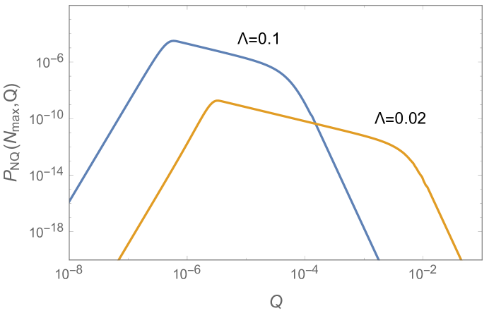
Figure 3: $P_{NQ}(N_{\rm max},Q)$ as a function of $Q$. We assume $N_{\rm max}=120$, $N_{\rm CMB}=50$, $U_{0}=10^{-19}$, $\bar{U}=0$, and $\Lambda=0.1$ (blue curve) or $0.02$ (orange curve).

In summary, the prior distribution (42) together with the condition (43) is the main result of this section. It can be written as $P_{NQ}(N_{\rm max},Q)\propto N_{\rm max}^{-3}P(Q)$ with

$$P(Q)\propto Q^{7} \qquad{\rm for}\ Q<Q_{1}$$ (51)

$$P(Q)\propto Q^{-1} \qquad{\rm for}\ Q_{1}<Q<Q_{2}$$ (52)

$$P(Q)\propto Q^{-9} \qquad{\rm for}\ Q_{2}<Q,$$ (53)

where $Q_{1}$ and $Q_{2}$ are defined in Eqs. (43) and (45), respectively. Substituting this into Eq. (34), we can calculate the probability distribution for observables in the multiverse, which will be discussed in Sec. 5. In the next section, we will show that Eq. (42) is still correct with some minor modifications in a higher-dimensional landscape.

4 A higher-dimensional Landscape

We now consider the probability distribution of $N_{\rm max}$ and $Q$ in a $D$-dimensional field space. We will see that the calculation reduces to the one-dimensional case with some minor modifications.

In a multi-field landscape, the Taylor expansion of the potential can be written as

$$U({\bm{\phi}})=U+\eta_{i}\phi_{i}+\frac{1}{2}\zeta_{ij}\phi_{i}\phi_{j}+\frac{1}{3!}\rho_{ijk}\phi_{i}\phi_{j}\phi_{k}+...,$$ (54)

where $i,j,k=1,2,...,D$. The expansion coefficients are $\eta_{i}=\partial U/\partial\phi_{i}$, $\zeta_{ij}=\partial U/\partial\phi_{i}\partial\phi_{j}$ and $\rho_{ijk}=\partial U/\partial\phi_{i}\partial\phi_{j}\partial\phi_{k}$, with all derivatives taken at ${\phi}_{i}=0$. Their typical values in the landscape are $\eta_{i}\sim U_{0}/\Lambda$, $\zeta_{ij}\sim U_{0}/\Lambda^{2}$, $\rho_{ijk}\sim U_{0}/\Lambda^{3}$.

Multi-field analogues of saddle points and inflection points can be defined as follows. A saddle point is a point where ${\partial}_{i}U=0$ and the Hessian matrix $\zeta_{ij}$ has one negative eigenvalue, with all other eigenvalues positive. An inflection point is a point where one of the Hessian eigenvalues is zero, with all other eigenvalues positive, and the gradient of $U({\bm{\phi}})$ vanishes in all directions orthogonal to that of the zero eigenvalue. Inflation is also possible at points with several negative or zero eigenvalues, but this occurs very rarely in a small-field landscape [14]. In the rest of the paper we shall disregard this possibility.

4.1 Inflection point inflation

We first consider a low-energy landscape with a fixed value of the average potential ${\bar{U}}$. Integration over ${\bar{U}}$ in Eq. (35) will be performed later. Ensemble averages over inflection (or saddle) points in the landscape can be calculated by integrating over ${\bm{\phi}}$ with appropriate delta functions $\prod_{i}\delta(f_{i}({\bm{\phi}}))$. Without loss of generality, we can diagonalize the Hessian, $\zeta_{ij}=\lambda_{i}\delta_{ij}$, and choose the $\phi_{1}$ axis in the direction of zero (or negative) eigenvalue. The slow roll will then occur essentially along the $\phi_{1}$ axis. To simplify the equations, we shall use the notation $\lambda\equiv\lambda_{1}$, $\eta\equiv\eta_{1}$, and $\rho\equiv\rho_{111}$.

Since for inflection points we require $\lambda=0$, $\lambda_{a}\geq 0$, and $\eta_{a}=0$ for $a=2,3,\dots,D$, we set $f_{1}({\bm{\phi}})=\lambda$ and $f_{a}({\bm{\phi}})=\eta_{a}$. The Jacobian associated with the delta functions is then given by $\left|\rho\prod_{a}\lambda_{a}\right|$. Hence the probability that inflection-point inflation with certain values of $N_{\rm max}$ and $Q$ will occur starting from a randomly chosen point in a landscape of average energy ${\bar{U}}$ is given by

$$P_{NQU}(N_{\rm max},Q,\bar{U})=\frac{D}{V}\int d^{D}\phi dU\prod_{i}d\eta_{i}\prod_{i}d\lambda_{i}\prod_{ijk}d\rho_{ijk}J(\lambda_{i}){\cal P}(U,\eta_{i},\lambda_{i},\rho_{ijk})f_{\rm vol}(U,\rho)\leavevmode\nobreak\ \delta(\lambda)|\rho|\times$$

$$\times\left(\prod_{a=2}^{D}\delta(\eta_{a})|\lambda_{a}|\right)\left(\prod_{a=2}^{D}\theta\left(\lambda_{a}\right)\right)\theta\left(\eta\rho\right)\theta(U)\delta\left(N_{\rm max}-\frac{\pi\sqrt{2}U}{\sqrt{\eta\rho}}\right)\delta\left(Q-\frac{N_{\rm CMB}^{2}\rho}{4\sqrt{3\pi}U^{1/2}}f(x,y)\right)$$ (55)

where we have included the volume factor $f_{\rm vol}\sim v_{0}U/(\Lambda\rho)$ . The combinatorial factor $D$ comes from selecting $\lambda_{1}$ to be the smallest eigenvalue. The integral $\int d^{D}\phi$ gives a volume in the field space $V$ because of the homogeneity of probability distribution ${\cal P}$. The Jacobian $J(\lambda_{i})$ comes from the variable transformation from $\zeta_{ij}$ to $\lambda_{i}$:

$$J(\lambda_{i})=C\prod_{i\neq j}\left|\lambda_{i}-\lambda_{j}\right|,$$ (56)

where $C$ is a constant. Finally the terms $\theta\left(\eta\rho\right)\theta(U)$ are included to ensure that slow roll is possible and does not lead to a shallow minimum. The distribution ${\cal P}(U,\eta_{i},\lambda_{i},\rho_{ijk})$ has the form

$${\cal P}(U,\eta_{i},\lambda_{i},\rho_{ijk})={\cal P}_{1}(U,\lambda_{i}){\cal P}_{2}(\eta_{i},\rho_{ijk})$$ (57)

$${\cal P}_{1}=A_{1}\exp[-{\cal Q}_{1}(U,\lambda_{i})]$$ (58)

$${\cal P}_{2}=A_{2}\exp[-{\cal Q}_{2}(\eta_{i},\rho_{ijk})],$$ (59)

where $A_{1}$ and $A_{2}$ are determined by the normalization conditions:

$$\int dU\prod_{i}d\lambda_{i}{\cal P}_{1}(U,\lambda_{i})=1$$ (60)

$$\int\prod_{i}d\eta_{i}\prod_{ijk}d\rho_{ijk}{\cal P}_{2}(\eta_{i},\rho_{ijk})=1.$$ (61)

The exponents ${\cal Q}_{1}(U,\lambda_{i})$ and ${\cal Q}_{2}(\eta_{i},\rho_{ijk})$ are given by [53, 27, 12]

$${\cal Q}_{1}(U,\lambda_{i})=c_{1}\frac{1}{U_{0}^{2}}(U-\bar{U})^{2}-c_{2}\frac{\Lambda^{2}}{DU_{0}^{2}}(U-\bar{U})\sum_{i}\lambda_{i}-c_{3}\frac{\Lambda^{4}}{DU_{0}^{2}}\left(\sum_{i}\lambda_{i}\right)^{2}+c_{4}\frac{\Lambda^{4}}{U_{0}^{2}}\lambda_{i}\lambda_{i}$$

$${\cal Q}_{2}(\eta_{i},\rho_{ijk})=c_{5}\frac{\Lambda^{2}}{U_{0}^{2}}\eta_{i}\eta_{i}+c_{6}\frac{\Lambda^{4}}{DU_{0}^{2}}\eta_{i}\rho_{ijj}-c_{7}\frac{\Lambda^{6}}{DU_{0}^{2}}\rho_{iik}\rho_{jjk}+c_{8}\frac{\Lambda^{6}}{U_{0}^{2}}\rho_{ijk}\rho_{ijk},$$ (62)

with summation over repeated indices. The coefficients $c_{i}$ can be expressed in terms of the moments of the correlation function and are typically $\mathcal{O}(1)$. Eq. (55) can be rewritten as

$$P_{NQU}(N_{\rm max},Q,\bar{U})=D\int dUd\eta d\lambda d\rho\leavevmode\nobreak\ {\cal P}_{1}^{\prime}(U,\lambda;\bar{U})\leavevmode\nobreak\ {\cal P}_{2}^{\prime}(\eta,\rho)\leavevmode\nobreak\ |\rho|\delta(\lambda)\leavevmode\nobreak\ f_{\rm vol}(U,\rho)\leavevmode\nobreak\ \theta(U)\theta\left(\eta\rho\right)$$

$$\leavevmode\nobreak\ \leavevmode\nobreak\ \leavevmode\nobreak\ \leavevmode\nobreak\ \leavevmode\nobreak\ \leavevmode\nobreak\ \leavevmode\nobreak\ \leavevmode\nobreak\ \leavevmode\nobreak\ \leavevmode\nobreak\ \leavevmode\nobreak\ \leavevmode\nobreak\ \leavevmode\nobreak\ \leavevmode\nobreak\ \leavevmode\nobreak\ \leavevmode\nobreak\ \leavevmode\nobreak\ \leavevmode\nobreak\ \leavevmode\nobreak\ \leavevmode\nobreak\ \leavevmode\nobreak\ \leavevmode\nobreak\ \leavevmode\nobreak\ \leavevmode\nobreak\ \times\leavevmode\nobreak\ \delta\left(N_{\rm max}-\frac{\pi\sqrt{2}U}{\sqrt{\eta\rho}}\right)\delta\left(Q-\frac{N_{\rm CMB}^{2}\rho}{4\sqrt{3\pi}U^{1/2}}f(x,y)\right),$$ (63)

where

$${\cal P}_{1}^{\prime}(U,\lambda;\bar{U})=\int\prod_{a=2}^{D}d\lambda_{a}{\cal P}_{1}(U,\lambda_{i})J(\lambda_{i})\prod_{a=2}^{D}|\lambda_{a}|\theta\left(\lambda_{a}\right),$$ (64)

$${\cal P}_{2}^{\prime}(\eta,\rho)=\int\prod_{a=2}^{D}d\eta_{a}\prod_{(ijk)\neq(111)}d\rho_{ijk}{\cal P}_{2}(\eta_{i},\rho_{ijk})\left(\prod_{a=2}^{D}\delta(\eta_{a})\right).$$ (65)

The delta function $\delta(\lambda)$ sets $\lambda=0$ in the distribution (64), while the other eigenvalues are integrated over. The resulting expression can be found using the saddle point method of Ref. [27]; it is given by

$${\cal P}_{1}^{\prime}(U,0;\bar{U})\sim\frac{U_{0}^{D-3}}{\Lambda^{2D-4}}\exp\left[-\left(d_{1}^{\prime}\frac{U-\bar{U}}{U_{0}}+d_{2}^{\prime}\sqrt{D}\right)^{2}-d_{3}^{\prime}\left(\frac{U-\bar{U}}{U_{0}}\right)^{2}\right],$$ (66)

where $d_{i}^{\prime}$ are ${\cal O}(1)$ constants. A detailed derivation of (66) will be discussed elsewhere [54].

The exponent of ${\cal P^{\prime}}_{2}$ is quadratic in all variables, so we can integrate $\eta_{a}$ ($a\geq 2$) and $\rho_{ijk}((i,j,k)\neq(111))$. We find that the coefficients of the remaining terms that are proportional to $\eta^{2}$ or $\rho^{2}$ do not change after the integration in the large $D$ limit. This is explained in detail in Appendix B. As a result, we have

$${\cal P}_{2}^{\prime}(\eta,\rho)\sim\frac{\Lambda^{D+3}}{U_{0}^{D+1}}\exp\left[-c_{5}\frac{\Lambda^{2}}{U_{0}^{2}}\eta^{2}-3c_{8}\frac{\Lambda^{6}}{U_{0}^{2}}\rho^{2}\right].$$ (67)

We are now ready to perform the integration over ${\bar{U}}$ in Eq. (35). In order to do that we first note that the dependence on ${\bar{U}}$ in $P_{NQU}(N_{\rm max},Q,\bar{U})$ is captured exclusively by ${\cal P}_{1}^{\prime}(U,0;\bar{U})$, so we just need to compute,

$${\cal P}_{1}^{\prime\prime}(U)=\int d\bar{U}P_{\rm cc}(0;\bar{U}){\cal P}_{1}^{\prime}(U,0;\bar{U})\sim\frac{\Lambda^{4}}{U_{0}^{2}}\frac{U_{0}^{D-1}}{\Lambda^{2D}}\exp\left[-c_{1}^{\prime}\frac{U^{2}}{U_{0}^{2}}\right]P^{\prime},$$ (68)

$$P^{\prime}\sim\exp\left[-d_{3}^{\prime\prime 2}D\right],$$ (69)

where $c_{1}^{\prime}$, $d_{3}^{\prime\prime}=\mathcal{O}(1)$. The exponential suppression factor $P^{\prime}$ is related to the fact that stationary points of index $(D-1)$ (that is, having all but one Hessian eigenvalues positive) are rather rare in the landscape.

After integration over $\eta$ and $\rho$, we obtain the following expression for the distribution $P_{NQ}$, which was defined in Eq. (35):

$$P_{NQ}(N_{\rm max},Q) = \int d\bar{U}P_{\rm cc}(0,\bar{U})P_{NQU}(N_{\rm max},Q,\bar{U})$$ (70)

$$= D\frac{4\pi^{5/2}v_{0}}{QN_{\rm max}^{3}}\int dUU^{3}\theta(U){\cal P}_{1}^{\prime\prime}(U){\cal P}_{2}^{\prime}(\eta_{*},\rho_{*}),$$ (71)

where $\eta_{*}$ and $\rho_{*}$ are the values (40) selected by the delta functions.

As before, $\eta_{*}$ is much smaller than the typical value $\eta_{0}\sim U_{0}/\Lambda$, so we can set $\eta_{*}\approx 0$ in the exponent of ${\cal P}_{2}^{\prime}$. We thus obtain

$$P_{NQ}(N_{\rm max},Q)\sim\frac{P^{\prime}}{\Lambda^{D}}\frac{Dv_{0}\Lambda^{7}}{U_{0}^{4}}\frac{1}{QN_{\rm max}^{3}}\int_{0}^{\infty}dUU^{3}\exp\left[-c_{1}^{\prime}\frac{U^{2}}{U_{0}^{2}}-3c_{8}\frac{\Lambda^{6}}{U_{0}^{2}}\rho_{*}^{2}\right],$$ (72)

We note that the factor $P^{\prime}/\Lambda^{D}$ is roughly the density of index-$(D-1)$ inflection points in the landscape.

Eq. (72) is very similar to Eq. (42) for the 1D case with ${\bar{U}}=0$. The difference is in the constant pre-factor and in ${\cal O}(1)$ coefficients in the exponent. Therefore, our results for the distribution of Q in Eqs. (44)-(48) should apply with these corrections.

In this Section we assumed, following the analysis in Ref. [14], that inflation in a multi-dimensional landscape is essentially single-field. This requires that all eigenvalues $\lambda_{j}$ of the Hessian matrix $\zeta_{ij}=\partial^{2}U/\partial\phi_{i}\partial\phi_{j}$ at the inflection point, apart from one zero eigenvalue, are large compared to the inflaton potential $U$. The typical value $\zeta_{ij}\sim U/\Lambda^{2}$ is much larger than $U$ for small values of $\Lambda$. In a higher-dimensional landscape, $D\gg 1$, some of the eigenvalues $\lambda_{j}$ may by chance be small. But for a sufficiently small $\Lambda$ we expect $1D$ inflation to be statistically prevalent. A careful analysis in Ref. [54] shows that this condition is satisfied if

$$\Lambda\ll D^{-1/4},$$ (73)

For $D\sim 100$, the condition is $\Lambda\ll 0.3$.

We note that inflation in random Gaussian models has been recently studied by Bjorkmo and Marsh [15], who concluded that multi-field effects are generically important in such models. The reason for this discrepancy is that the landscape properties assumed in Ref. [15] are significantly different from ours. The most significant difference is that they assume that the correlation function has a Gaussian form, $F(x)\propto\exp(-x^{2}/2)$. This is a rather special case, in which the distribution of Hessian eigenvalues at a stationary point has a sharp peak around zero, so it is not surprising that some fields are light enough to be excited during inflation [54]. On the other hand, we assumed a generic correlation function, which does not have this property. Moreover, in most of their numerical examples Bjorkmo and Marsh used the parameters $\Lambda\ =0.4$ and $N\leq 100$, which do not satisfy the condition (73).

4.2 Saddle point inflation

For saddle point inflation, the analogue of the distribution (55) is

$$P_{NQU}(N_{\rm max},Q,{\bar{U}})=\frac{D}{V}\int\dots\int d^{D}\phi dU\prod_{i}d\eta_{i}\prod_{i}d\lambda_{i}\prod_{ijk}d\rho_{ijk}J(\lambda_{i}){\cal P}(U,\eta_{i},\lambda_{i},\rho_{ijk})f_{\rm vol}(U,\rho)$$

$$\times\delta(\eta)|\lambda|\left(\prod_{a=2}^{D}\delta(\eta_{a})|\lambda_{a}|\right)\left(\prod_{a=2}^{D}\theta\left(\lambda_{a}\right)\right)\theta\left(-\lambda\right)\theta(U)\delta\left(N_{\rm max}-\frac{2\pi U}{\left|\lambda\right|}\right)\delta\left(Q-\frac{N_{\rm CMB}^{2}\rho}{4\sqrt{3\pi}U^{1/2}}f(x,y)\right),$$

where $f_{\rm vol}(U,\rho)\sim U/\rho$.

The delta functions fix $\lambda$ and $\rho$ to the values

$$\lambda_{*}(U)=\frac{2\pi U}{N_{\rm max}},\leavevmode\nobreak\ \leavevmode\nobreak\ \leavevmode\nobreak\ \leavevmode\nobreak\ \rho_{*}(U)=\frac{4\sqrt{3\pi}QU^{1/2}}{N_{\rm CMB}^{2}f(x,y)}.$$ (74)

The slow roll condition requires $\lambda_{*}<U\lesssim U_{0}$, which is much smaller than the typical value of $\lambda$. Hence we can set $\lambda_{*}\approx 0$ in the exponent of ${\cal P}$.

The remaining integrals can be evaluated following the same steps as in the preceding subsection, with only minor changes. For example, ${\cal P}_{1}^{\prime}(U,0;\bar{U})$ is now replaced with ${\cal P}_{1}^{\prime}(U,\lambda_{*};\bar{U})$. This change, however, has little effect on the distribution. It was shown in Ref. [54] that with $\lambda_{1}\approx 0$, the second smallest eigenvalue of the Hessian is of the order $\lambda_{2}\sim U_{0}/(\sqrt{D}\Lambda^{2})$. This is much greater than $\lambda_{*}$ if $\Lambda\ll D^{-1/4}\approx 0.3$ (for $D\sim 100$). Then the Jacobian $J(\lambda_{i})$ in Eq. (56) changes very little when we replace $\lambda_{1}=0$ by $\lambda_{*}$, so we can estimate

$${\cal P}_{1}^{\prime}(U,\lambda_{*};\bar{U})\sim{\cal P}_{1}^{\prime}(U,0;\bar{U}).$$ (75)

After integration over $\bar{U}$, we finally obtain

$$P_{NQ}(N_{\rm max},Q) \sim D\frac{1}{\sqrt{2\pi}}\frac{4\pi^{5/2}}{QN_{\rm max}^{3}}\int_{0}^{\infty}dUU^{3}{\cal P}_{1}^{\prime\prime}(U){\cal P}_{2}^{\prime}(0,\rho_{*})$$ (76)

$$\sim \frac{P^{\prime}}{\Lambda^{D}}\frac{D\Lambda^{7}}{U_{0}^{4}}\frac{1}{QN_{\rm max}^{3}}\int_{0}^{\infty}dUU^{3}\exp\left[-c_{1}^{\prime}\frac{U^{2}}{U_{0}^{2}}-3c_{8}\frac{\Lambda^{6}}{U_{0}^{2}}\rho_{*}^{2}\right].$$ (77)

This is the same as Eq. (72) but without a factor of $v_{0}$ and with a different $f(x,y)$ in $\rho_{*}(U)$ (see Appendix A). Note that $f(x,y)\simeq 1$ for $N_{\rm max}\gtrsim N_{\rm CMB}$ and the difference is small in this case, because the observable scale leaves the horizon when the potential is dominated by the cubic term. Thus the probability of saddle point inflation is suppressed by a factor of $1/v_{0}$ ($\sim 0.06$) compared with that of inflection point inflation with the same $N_{\rm max}$ and $Q$.

5 Observational predictions

Our main result is that the “prior” probability distribution in Eq. (34) has the form

$$P_{NQ}(N_{\rm max},Q)\propto N_{\rm max}^{-3}P(Q)$$ (78)

with

$$P(Q)\propto Q^{-1}.$$ (79)

It applies in the range $Q_{1}<Q<Q_{2}$, where $Q_{1}$ and $Q_{2}$ are defined in Eqs. (43) and (45), respectively. Outside of this range, $P(Q)$ rapidly declines towards zero.

To derive observational predictions, we also need to know the anthropic factor $n^{\rm(obs)}(N_{\rm max},Q,\rho_{v})$ in Eq. (34). We will not attempt a detailed analysis here and will only give a rough outline of the observational implications of Eqs. (78),(79).

”Pocket universes” resulting from bubble nucleation have negative spatial curvature, which depends on the number of e-folds of inflation in the bubble, $N_{e}\lesssim N_{\rm max}$. The $N_{\rm max}$ dependence in Eq. (78) disfavors large values of $N_{\rm max}$ and thus favors large magnitude of the curvature. On the other hand, if the curvature is so large that it suppresses structure formation, the density of observers is also suppressed. This gives an anthropic upper bound on the magnitude of curvature and a lower bound on $N_{e}$ [55, 56]. It was noted in Ref. [56] that these bounds are rather close to the observational bounds. For example, in models where inflation is at a GUT scale and thermalization is instantaneous, the anthropic bound is $N_{e}\gtrsim 60$, while the observational bound is $N_{e}>62$. This is consistent with the distribution (78), which suggests that $N_{e}$ should be close to the smallest anthropically allowed value.

Anthropic bounds on the amplitude of density perturbations $Q$ have been discussed in Refs. [57, 58], with the conclusion that both lower and upper bounds are within an order of magnitude of the observed value $Q^{\rm(obs)}\sim 10^{-4}$. If $Q^{\rm(obs)}$ were smaller than $Q_{1}$ or larger than $Q_{2}$, it would be in the range where $P(Q)$ changes very rapidly. The expected value of $Q$ would then be pushed into the anthropically unfavorable territory, so finding $Q\sim Q_{\rm obs}$, which is comfortably within the anthropically favored zone, would be rather unlikely. We thus conclude that the observed value of $Q\sim 10^{-4}$ should be within the range of $(Q_{1},Q_{2})$, which requires

$$\frac{U_{0}}{\Lambda^{2}}\lesssim 10^{-13}\lesssim\frac{U_{0}}{\Lambda^{6}}.$$ (80)

This gives a restriction on observationally acceptable models of random Gaussian landscape.

Assuming $Q_{1}<Q^{\rm(obs)}<Q_{2}$, we next estimate the anthropic factor $n^{\rm(obs)}(N_{\rm max},Q,\rho_{v})$ in more detail.

The observer density $n^{\rm(obs)}$ is expected to be roughly proportional to the fraction of matter $f_{G}$ clustered in large galaxies (with mass $M\gtrsim 10^{11}M_{\odot}$). The idea is that there is a certain number of stars per unit mass in a galaxy and certain number of observers per star. The mass fraction $f_{G}$ can be found in the Press-Schechter approximation. Restricting attention to positive values of $\rho_{v}$ and assuming that $N_{\rm max}$ is large enough to yield a nearly flat universe, it is given by [59, 60]

$$f_{G}\propto{\rm erfc}\left[0.8\left(\frac{\rho_{v}}{\rho_{m}\sigma_{G}^{3}}\right)^{1/3}\right],$$ (81)

where $\rho_{m}$ is the density of nonrelativistic matter and $\sigma_{G}$ is the linearized density contrast on the galactic scale. $\sigma_{G}$ is linearly related to the primordial fluctuation amplitude $Q$, $\sigma_{G}\propto Q$. The product $\rho_{m}\sigma_{G}^{3}$ is time-independent during the matter era and can be evaluated at any time.

From Eqs. (79) and (81), the combined probability distribution for $\rho_{v}$ and $Q$ in the multiverse can be written as

$$dP(\rho_{v},Q)\propto\frac{dQ}{Q}{\rm erfc}(0.8\xi^{1/3})d\rho_{v},$$ (82)

where

$$\xi\equiv\frac{\rho_{v}}{\rho_{m}\sigma_{G}^{3}}\propto\frac{\rho_{v}}{Q^{3}}.$$ (83)

With a change of variables $\{Q,\rho_{v}\}\to\{Q,\xi\}$, this distribution factorizes [61]:

$$dP(\xi,Q)\propto Q^{2}{dQ}\times{\rm erfc}(0.8\xi^{1/3})d\xi$$ (84)

The distribution for $\xi$ is peaked at $\xi\sim 1$ (on a logarithmic scale of $\xi$). With $Q\sim 10^{-4}$, the corresponding value of $\rho_{v}$ is comparable to the observed value $\rho_{v}^{(0)}$. But more generally, this distribution predicts the value of $\rho_{v}/Q^{3}$.

The novel aspect of Eq. (84) is the distribution for $Q$. This distribution applies in the range from $Q_{1}$ to $Q_{2}$; hence it is peaked at $Q_{2}$.

In the above analysis we made a number of simplifications, which we shall now spell out.

(i) $f_{G}$ in Eq. (81) is the asymptotic mass fraction, while in the scale factor measure we need to use the density of observers at a finite time $t_{\rm obs}$. This distinction, however, has little effect on the probability distribution.

(ii) In the scale-factor measure, the distribution (82) has an additional factor $\sim\exp(-3H_{v}t_{\rm obs})$, which arises due to the change in the expansion rate after vacuum energy domination [37, 38]. Here, $H_{v}=(\rho_{v}/3)^{1/2}$ is the expansion rate during the vacuum dominated epoch. This factor suppresses large values of $\rho_{v}$, but its effect is not very significant for observationally interesting values of $\rho_{v}$ and $t_{\rm obs}$.

(iii) The density of observers can be influenced by a number of other factors that we have not included here. For example, regions with large values of $Q$ may be disfavored due to life extinctions caused by close encounters with stars or molecular clouds [57]. If the dangerous value $Q_{*}$ above which this effect is significant is $Q_{*}<Q_{2}$, we can expect to observe $Q\sim Q_{*}$, which means that the rate of extinctions is close to the dangerous level. This prediction is consistent with the fact that great extinctions on Earth occurred once in $\sim 10^{8}$ years, which is about the time that it took intelligent life to evolve. Life extinctions could also be caused by gamma-ray bursts. This could suppress the probability of very small and negative values of $\rho_{v}$ [62].

6 Conclusions and discussion

The idea that the Landscape of String Theory can be composed of more than one sectors of the moduli space with different energy scales motivates the study of the cosmological implications of a random landscape with this structure. In this paper we have assumed that there are two distinct sectors of the landscape with a hierarchy of energies, a low energy and a high-energy scale. This type of model captures some of the key features of string theory compactifications, however, it is still a toy model and the specific form of the potential found in the literature may be different from the one we present here. Nevertheless we believe the conclusions of this paper will be also applicable for more realistic models of compactification.

With this structure of the landscape, we have shown that the initial conditions for our primordial universe are likely to be determined by quantum tunneling between the vacua in the field space of the high energy sector. Moreover, the field values of the low energy moduli sector do not change much due to this quantum tunneling process. Since we do not expect strong correlations between the potentials of these fields, the initial values of the fields in the low energy sector would have a flat distribution. The subsequent cosmological evolution inside the bubble is mostly determined by the dynamics of the low energy landscape sector. Inflationary periods in this sector would be dominated by trajectories that fall within the attractor region of fine tuned inflection points and saddle points of the landscape.

This picture allowed us to compute the probability distribution for the (maximal) number of e-folds $N_{\rm max}$, the amplitude of scalar fluctuations $Q$, and the vacuum energy density $\rho_{v}$ in the multiverse for this model. The resulting distribution can be represented as

$$dP\propto P_{\rm prior}n_{\rm obs}dN_{\rm max}dQd\rho_{v},$$ (85)

where the prior distribution has the form

$$P_{\rm prior}(N_{\rm max},Q)\propto N_{\rm max}^{-3}P(Q)$$ (86)

and is (to a good approximation) independent of $\rho_{v}$. We found that the distribution for $Q$ in Eq. (86) is $P(Q)\propto Q^{-1}$ in the range $Q_{1}<Q<Q_{2}$, with $Q_{1}$ and $Q_{2}$ respectively given by Eqs. (43) and (45), and drops rapidly towards zero outside of this range. Requiring that the observed value of $Q$ falls between $Q_{1}$ and $Q_{2}$, we obtained a constraint on the model parameters, Eq. (80). We also found that the probability of saddle point inflation is smaller than that of inflection point inflation, roughly by an order of magnitude.

The prior distribution specified above is the main result of this paper. We also briefly discussed the anthropic factor $n^{(\rm obs)}(N_{\rm max},Q,\rho_{v})$. The number of e-folds $N_{\rm max}$ should be large enough, so that curvature does not dominate prior to galaxy formation. Since $P_{\rm prior}$ is a decreasing function of $N_{\rm max}$, we expect that the observed value of $N_{\rm max}$ should be comparable to this anthropic bound. Disregarding the $N_{\rm max}$-dependence, the full distribution for $\rho_{v}$ and $Q$ (including the anthropic factor) can be represented in a factorized form

$$dP(\xi,Q)\propto Q^{2}{dQ}\leavevmode\nobreak\ F(\xi)d\xi,$$ (87)

where $\xi\propto\rho_{v}/Q^{3}$. The new variable $\xi$ and the function $F$ are specified in Sec. 5. The value of $\xi$ corresponding to the observed value of the combination $\rho_{v}/Q^{3}$ is close to the peak of the function $F(\xi)$. This manifests the celebrated anthropic solution of the cosmological constant problem. The novel aspect of Eq. (87) is the distribution for $Q$, which applies in the range $Q_{1}<Q<Q_{2}$.

While we used a random Gaussian model to describe the low-energy landscape $U_{\rm L}({\bf\phi},{\bf\psi})$, our conclusions are rather insensitive to the assumptions about the high-energy landscape $U_{\rm H}({\bf\psi})$. We only used three assumptions regarding the high-energy landscape: (i) that the tunneling rate in the potential $U_{\rm H}({\bf\psi})$ is much higher than that in $U_{\rm L}$, (ii) that the tunneling points are uncorrelated with the low-energy potential, and (iii) that the distribution of vacuum energy densities in $U_{\rm H}$ is much wider than $U_{\rm L}$. These assumptions are likely to be satisfied in a very wide class of models.

Our conclusions may also be applicable to one-scale models with $U_{\rm H}=U_{\rm L}$ under an additional condition. In our calculations, we used the facts that the initial condition for slow-roll inflation has a flat distribution in the low-energy landscape and that the volume of the attractor region $f_{\rm vol}$ is independent of the dimension of landscape. These are true even for one-scale models with $U_{\rm H}=U_{\rm L}$ if the dependence of the tunneling rate on the tunneling point in the attractor region is negligible. In this case, the tunneling probability is peaked along the slow-roll direction [14] and the length of the slow-roll track is $(v_{0}U/\rho)$, which is parametrically equal to $f_{\rm vol}$. The condition can then be written as $1\gg(v_{0}U/\rho)\cdot dS/d\phi$. The factor of $dS/d\phi$ can be roughly estimated as $(\Lambda^{4}/U)\bar{S}/\Lambda$ from Eq. (8), where $\bar{S}\gtrsim{\cal O}(10)$. The parameter $\rho$ can be rewritten in terms of $Q$ and $U^{1/2}$ from Eq. (40) and $U$ is $\sim U_{0}$ in the anthropically allowed range we are interested in. As a result, the condition can be rewritten as $U_{0}/\Lambda^{6}\gg v_{0}^{2}f^{2}N_{\rm CMB}^{4}\bar{S}^{2}/(48\pi Q^{2})\sim 10^{17}$ for $Q\sim 10^{-4}$. Hence our conclusions are applicable also to one-scale models with $U_{0}/\Lambda^{6}\gg 10^{17}$.

The methods we used here can be applied to other models, in particular to the random $\alpha$-attractor model recently introduced in Ref. [46]. In this model some directions have a flat potential due to a singularity of their kinetic terms, so that the effective mass in those directions is much smaller than that in the perpendicular directions. Some of our results and methods may also be applicable to axionic landscapes which have been studied recently in Ref. [63].

Appendix A Observables of Inflation

In this Appendix we review the derivation of spectral index $n_{s}$ and amplitude of scalar fluctuations $Q$ in inflection point inflation and saddle point inflation.

A.1 Inflection point inflation

The potential for inflection point inflation is

$$U(\phi)=U+\eta\phi+\frac{1}{3!}\rho\phi^{3}+...,$$ (88)

where $\eta\rho>0$. The slow roll ends when $|U^{\prime\prime}|/U=1$, or

$$\phi_{\rm end}=-U/\rho.$$ (89)

The number of e-folds from the observable scale $\phi$ to $\phi_{\rm end}$ should be $N_{\rm CMB}\sim 50$:

$$N_{\rm CMB} = -\int_{\phi}^{\phi_{\rm end}}d\phi\frac{U(\phi)}{U^{\prime}(\phi)}$$ (90)

$$\simeq \frac{N_{\rm max}}{\pi}{\rm Arctan}\left[\frac{\sqrt{\rho/2\eta}(\phi_{\rm end}-\phi)}{1+(\rho/2\eta)\phi\phi_{\rm end}}\right],$$ (91)

where we assume $U(\phi)\simeq U$ in the denominator. Here the maximal number of e-folds $N_{\rm max}$ is given by

$$N_{\rm max}=-\int_{-\phi_{\rm end}}^{\phi_{\rm end}}d\phi\frac{U(\phi)}{U^{\prime}(\phi)}\approx\pi\sqrt{2}\frac{U}{\sqrt{\eta\rho}}.$$ (92)

The field value $\phi$ at which the CMB scale leaves the horizon is therefore given by

$$\sqrt{\frac{\rho}{2\eta}}\phi=-\frac{\tan x+y}{1-y\tan x},$$ (93)

where

$$x\equiv\pi\frac{N_{\rm CMB}}{N_{\rm max}}$$ (94)

$$y\equiv\frac{N_{\rm max}}{2\pi}.$$ (95)

The spectral index is given by

$$1-n_{s} = 6\cdot\frac{1}{2}\left(\frac{U^{\prime}(\phi)}{U}\right)^{2}-2\left(\frac{U^{\prime\prime}(\phi)}{U}\right)$$ (96)

$$\simeq -\frac{2\rho\phi}{U}=\frac{2}{y}\frac{y+\tan x}{y\tan x-1},$$ (97)

where we neglect the first term in the first line.

The magnitude of density fluctuations produced at $\phi$ is

$$Q^{2} = \frac{1}{12\pi}\frac{U^{3}(\phi)}{{U^{\prime}}^{2}(\phi)}$$ (98)

$$\simeq \frac{U^{3}}{12\pi\eta^{2}}\frac{\left(1-y\tan x\right)^{4}}{\left[\left(1-y\tan x\right)^{2}+\left(\tan x+y\right)^{2}\right]^{2}}.$$ (99)

This can be rewritten as

$$Q^{2}\simeq\frac{N_{\rm CMB}^{4}\rho^{2}}{48\pi U}f^{2}(x,y)$$ (100)

$$f(x,y)\equiv\frac{\cos^{2}x\left(y\tan x-1\right)^{2}}{x^{2}\left(y^{2}+1\right)}.$$ (101)

Note that $x$ and $y$ depend only on $N_{\rm max}$. Note also that $f(x,y)\simeq 1$ for $N_{\rm max}\gtrsim N_{\rm CMB}\gg 1$. Also, $f(x,y)\sim 1$ for $y\gg 1$ and $x\sim 1$.

A.2 Saddle point inflation

The potential for saddle point inflation is

$$U(\phi)=U+\frac{1}{2}\lambda\phi^{2}+\frac{1}{3!}\rho\phi^{3}+...,$$ (102)

where $\lambda<0$. The slow roll ends when $|U^{\prime\prime}|/U=1$, or

$$\phi_{\rm end}=-\frac{U+\lambda}{\rho}.$$ (103)

The number of e-folds from the observable scale $\phi$ to $\phi_{\rm end}$ should be $N_{\rm CMB}\sim 50$:

$$N_{\rm CMB}\simeq\frac{U}{\left|\lambda\right|}\ln\left(\frac{\phi}{\phi_{\rm end}}\frac{1-\rho\phi_{\rm end}/2\left|\lambda\right|}{1-\rho\phi/2\left|\lambda\right|}\right).$$ (104)

Here the “maximal number of e-folds” $N_{\rm max}$ is defined by

$$N_{\rm max}\equiv 2\pi\frac{U}{\left|\lambda\right|}.$$ (105)

The field value $\phi$ at which the CMB scale leaves the horizon is therefore given by

$$\frac{\rho}{2\left|\lambda\right|}\phi\simeq-\frac{(y-1)e^{x}}{(y+1)e^{-x}-(y-1)e^{x}},$$ (106)

where we use $\rho\phi_{\rm end}/2\left|\lambda\right|=-(y-1)/2$, and $x$ and $y$ are defined by Eqs. (94) and (95), respectively.

The spectral index is given by

$$1-n_{s} = 6\cdot\frac{1}{2}\left(\frac{U^{\prime}(\phi)}{U}\right)^{2}-2\left(\frac{U^{\prime\prime}(\phi)}{U}\right)$$ (107)

$$\simeq -2\frac{\lambda+\rho\phi}{U}=\frac{2}{y}\frac{y-\tanh x}{y\tanh x-1},$$ (108)

where we neglect the first term in the first line.

The magnitude of density fluctuations produced at $\phi$ is

$$Q^{2} \simeq \frac{U^{3}}{12\pi\lambda^{2}}\frac{\rho^{2}}{4\lambda^{2}}\frac{\left[(y+1)e^{-x}-(y-1)e^{x}\right]^{4}}{\left[(y-1)e^{x}\right]^{2}\left[(y+1)e^{-x}\right]^{2}},$$ (109)

This can be rewritten as

$$Q^{2}\simeq\frac{N_{\rm CMB}^{4}\rho^{2}}{48\pi U}f^{2}(x,y)$$ (110)

$$f(x,y)\equiv\frac{\cosh^{2}x\left(y\tanh x-1\right)^{2}}{x^{2}\left(y^{2}-1\right)}.$$ (111)

Note again that $x$ and $y$ depend only on $N_{\rm max}$ and $f(x,y)\to 1$ for $N_{\rm max}\gtrsim N_{\rm CMB}\gg 1$.

Appendix B Calculation of ${\cal P}_{2}^{\prime}(\eta,\rho)$

In this Appendix we calculate ${\cal P}_{2}^{\prime}(\eta,\rho)$ in a large $D$ limit. Explicitly, it is given by

$${\cal P}_{2}^{\prime}(\eta,\rho)=A_{2}\int\prod_{(ijk)\neq(111)}d\rho_{ijk}\exp\left[-c_{5}\frac{\Lambda^{2}}{U_{0}^{2}}\eta\eta-c_{6}\frac{\Lambda^{4}}{DU_{0}^{2}}\eta\rho_{1ii}+c_{7}\frac{\Lambda^{6}}{DU_{0}^{2}}\rho_{iik}\rho_{jjk}-c_{8}\frac{\Lambda^{6}}{U_{0}^{2}}\rho_{ijk}\rho_{ijk}\right]\leavevmode\nobreak\ ,$$

where we have performed the integrals of the delta functions. Since we are interested in the distribution of $\eta$ and $\rho$, the integrals of $\rho_{ijk}$ with $i<j<k$, $1<i\neq j=k$, or their permutations can be absorbed into the normalization factor. Then we obtain

$${\cal P}_{2}^{\prime}(\eta,\rho)=A_{2}^{\prime}\int\prod_{a\geq 2}d\rho_{1aa}\exp\left[-c_{5}\frac{\Lambda^{2}}{U_{0}^{2}}\eta\eta-c_{6}\frac{\Lambda^{4}}{DU_{0}^{2}}\eta\rho_{1ii}+c_{7}\frac{\Lambda^{6}}{DU_{0}^{2}}\rho_{1ii}\rho_{1jj}-3c_{8}\frac{\Lambda^{6}}{U_{0}^{2}}\sum_{i}\rho_{1ii}\rho_{1ii}\right]\leavevmode\nobreak\ ,$$

This is Gaussian integrals of $D-1$ variables $\rho_{1aa}$ ($a\geq 2$). The result is given by

$${\cal P}_{2}^{\prime}(\eta,\rho)=A_{2}^{\prime\prime}\exp\left[-c_{5}\frac{\Lambda^{2}}{U_{0}^{2}}\eta^{2}-c_{6}\frac{\Lambda^{4}}{DU_{0}^{2}}\eta\rho-(3c_{8}-c_{7}/D)\frac{\Lambda^{6}}{U_{0}^{2}}\rho^{2}+C(\eta,\rho)\right],$$ (112)

where $C(\eta,\rho)$ comes from the integrals of $\rho_{1aa}$:

$$C(\eta,\rho)=\left(\frac{1}{D(3c_{8}D-c_{7}(D-1))}\right)\left(\frac{c_{6}^{2}}{4}\frac{\Lambda^{2}}{U_{0}^{2}}\eta^{2}-c_{6}c_{7}\frac{\Lambda^{2}}{U_{0}^{4}}\eta\rho+c_{7}^{2}\frac{\Lambda^{2}}{U_{0}^{6}}\rho^{2}\right).$$ (113)

Since $C(\eta,\rho)$ is suppressed by $1/D^{2}$, we can neglect it in a large $D$ limit. The normalization constant can be easily determined by the dimensional analysis. Note first that ${\cal P}_{2}(\eta_{i},\rho_{ijk})$ is normalized as Eq. (61). On the other hand, $\eta$ and $\rho$ are not integrated out in ${\cal P}_{2}^{\prime}$ and there are $\prod_{a\geq 2}\delta(\eta_{i})$ in Eq. (65) for ${\cal P}_{2}^{\prime}(\eta,\rho)$. So there should be a factor of $(U_{0}/\Lambda)^{-1}*(U_{0}/\Lambda^{3})^{-1}*(U_{0}/\Lambda)^{-(D-1)}$. Thus we estimate

$$A_{2}^{\prime\prime}\sim\frac{\Lambda^{D+3}}{U_{0}^{D+1}}.$$ (114)

References

- [1] M. R. Douglas and S. Kachru, Flux compactification, Rev. Mod. Phys. 79 (2007) 733 [hep-th/0610102].
- [2] R. Bousso and J. Polchinski, Quantization of four form fluxes and dynamical neutralization of the cosmological constant, JHEP 06 (2000) 006 [hep-th/0004134].
- [3] M. Tegmark, What does inflation really predict?, JCAP 0504 (2005) 001 [astro-ph/0410281].
- [4] A. Aazami and R. Easther, Cosmology from random multifield potentials, JCAP 0603 (2006) 013 [hep-th/0512050].
- [5] J. Frazer and A. R. Liddle, Exploring a string-like landscape, JCAP 1102 (2011) 026 [1101.1619].
- [6] D. Battefeld, T. Battefeld and S. Schulz, On the Unlikeliness of Multi-Field Inflation: Bounded Random Potentials and our Vacuum, JCAP 1206 (2012) 034 [1203.3941].
- [7] I.-S. Yang, Probability of Slowroll Inflation in the Multiverse, Phys. Rev. D86 (2012) 103537 [1208.3821].
- [8] T. C. Bachlechner, On Gaussian Random Supergravity, JHEP 04 (2014) 054 [1401.6187].
- [9] G. Wang and T. Battefeld, Vacuum Selection on Axionic Landscapes, JCAP 1604 (2016) 025 [1512.04224].
- [10] A. Masoumi and A. Vilenkin, Vacuum statistics and stability in axionic landscapes, JCAP 1603 (2016) 054 [1601.01662].
- [11] R. Easther, A. H. Guth and A. Masoumi, Counting Vacua in Random Landscapes, 1612.05224.
- [12] A. Masoumi, A. Vilenkin and M. Yamada, Inflation in random Gaussian landscapes, JCAP 1705 (2017) 053 [1612.03960].
- [13] A. Masoumi, A. Vilenkin and M. Yamada, Initial conditions for slow-roll inflation in a random Gaussian landscape, JCAP 1707 (2017) 003 [1704.06994].
- [14] A. Masoumi, A. Vilenkin and M. Yamada, Inflation in multi-field random Gaussian landscapes, JCAP 1712 (2017) 035 [1707.03520].
- [15] T. Bjorkmo and M. C. D. Marsh, Manyfield Inflation in Random Potentials, JCAP 1802 (2018) 037 [1709.10076].
- [16] M. C. D. Marsh, L. McAllister, E. Pajer and T. Wrase, Charting an Inflationary Landscape with Random Matrix Theory, JCAP 1311 (2013) 040 [1307.3559].
- [17] M. Dias, J. Frazer and M. C. D. Marsh, Simple emergent power spectra from complex inflationary physics, Phys. Rev. Lett. 117 (2016) 141303 [1604.05970].
- [18] G. Wang and T. Battefeld, Random Functions via Dyson Brownian Motion: Progress and Problems, JCAP 1609 (2016) 008 [1607.02514].
- [19] B. Freivogel, R. Gobbetti, E. Pajer and I.-S. Yang, Inflation on a Slippery Slope, 1608.00041.
- [20] F. G. Pedro and A. Westphal, Inflation with a graceful exit in a random landscape, JHEP 03 (2017) 163 [1611.07059].
- [21] M. Dias, J. Frazer and M. c. D. Marsh, Seven Lessons from Manyfield Inflation in Random Potentials, JCAP 1801 (2018) 036 [1706.03774].
- [22] J. J. Blanco-Pillado, M. Gomez-Reino and K. Metallinos, Accidental Inflation in the Landscape, JCAP 1302 (2013) 034 [1209.0796].
- [23] K. Metallinos, Numerical exploration of the string theory landscape, Phd Thesis, ProQuest Dissertations and Theses 75-02(E) (2013) 114.
- [24] D. Martinez-Pedrera, D. Mehta, M. Rummel and A. Westphal, Finding all flux vacua in an explicit example, JHEP 06 (2013) 110 [1212.4530].
- [25] J. P. Conlon, F. Quevedo and K. Suruliz, Large-volume flux compactifications: Moduli spectrum and D3/D7 soft supersymmetry breaking, JHEP 08 (2005) 007 [hep-th/0505076].
- [26] D. Gallego and M. Serone, An Effective Description of the Landscape. I., JHEP 01 (2009) 056 [0812.0369].
- [27] A. J. Bray and D. S. Dean, Statistics of critical points of Gaussian fields on large-dimensional spaces, Phys. Rev. Lett. 98 (2007) 150201.
- [28] G. R. Dvali and A. Vilenkin, Field theory models for variable cosmological constant, Phys. Rev. D64 (2001) 063509 [hep-th/0102142].
- [29] G. Dvali, Large hierarchies from attractor vacua, Phys. Rev. D74 (2006) 025018 [hep-th/0410286].
- [30] C. Brodie and M. C. D. Marsh, The Spectra of Type IIB Flux Compactifications at Large Complex Structure, JHEP 01 (2016) 037 [1509.06761].
- [31] M. C. D. Marsh and K. Sousa, Universal Properties of Type IIB and F-theory Flux Compactifications at Large Complex Structure, JHEP 03 (2016) 064 [1512.08549].
- [32] M. Dine and N. Seiberg, Is the Superstring Weakly Coupled?, Phys. Lett. 162B (1985) 299.
- [33] T. C. Bachlechner, Inflation Expels Runaways, JHEP 12 (2016) 155 [1608.07576].
- [34] B. Freivogel, Making predictions in the multiverse, Class. Quant. Grav. 28 (2011) 204007 [1105.0244].
- [35] A. D. Linde and A. Mezhlumian, Stationary universe, Phys. Lett. B307 (1993) 25 [gr-qc/9304015].
- [36] A. D. Linde, D. A. Linde and A. Mezhlumian, From the Big Bang theory to the theory of a stationary universe, Phys. Rev. D49 (1994) 1783 [gr-qc/9306035].
- [37] A. De Simone, A. H. Guth, M. P. Salem and A. Vilenkin, Predicting the cosmological constant with the scale-factor cutoff measure, Phys. Rev. D78 (2008) 063520 [0805.2173].
- [38] R. Bousso, B. Freivogel and I.-S. Yang, Properties of the scale factor measure, Phys. Rev. D79 (2009) 063513 [0808.3770].
- [39] J. Garriga and A. Vilenkin, Watchers of the multiverse, JCAP 1305 (2013) 037 [1210.7540].
- [40] A. Vilenkin, A quantum measure of the multiverse, JCAP 1405 (2014) 005 [1312.0682].
- [41] A. De Simone, A. H. Guth, A. D. Linde, M. Noorbala, M. P. Salem and A. Vilenkin, Boltzmann brains and the scale-factor cutoff measure of the multiverse, Phys. Rev. D82 (2010) 063520 [0808.3778].
- [42] J. Garriga and A. Vilenkin, Recycling universe, Phys. Rev. D57 (1998) 2230 [astro-ph/9707292].
- [43] J. Garriga, D. Schwartz-Perlov, A. Vilenkin and S. Winitzki, Probabilities in the inflationary multiverse, JCAP 0601 (2006) 017 [hep-th/0509184].
- [44] J. Garriga, A. Vilenkin and J. Zhang, Non-singular bounce transitions in the multiverse, JCAP 1311 (2013) 055 [1309.2847].
- [45] A. Masoumi, K. D. Olum and B. Shlaer, Efficient numerical solution to vacuum decay with many fields, JCAP 1701 (2017) 051 [1610.06594].
- [46] A. Linde, Random Potentials and Cosmological Attractors, JCAP 1702 (2017) 028 [1612.04505].
- [47] S. Weinberg, Anthropic Bound on the Cosmological Constant, Phys. Rev. Lett. 59 (1987) 2607.
- [48] S. Weinberg, The Cosmological Constant Problem, Rev. Mod. Phys. 61 (1989) 1.
- [49] A. D. Linde and A. Westphal, Accidental Inflation in String Theory, JCAP 0803 (2008) 005 [0712.1610].
- [50] D. Baumann, A. Dymarsky, I. R. Klebanov and L. McAllister, Towards an Explicit Model of D-brane Inflation, JCAP 0801 (2008) 024 [0706.0360].
- [51] A. Vilenkin, The Birth of Inflationary Universes, Phys. Rev. D27 (1983) 2848.
- [52] N. Agarwal, R. Bean, L. McAllister and G. Xu, Universality in D-brane Inflation, JCAP 1109 (2011) 002 [1103.2775].
- [53] Y. V. Fyodorov, Complexity of Random Energy Landscapes, Glass Transition and Absolute Value of Spectral Determinant of Random Matrices, Phys. Rev. Lett. 92 (2004) .
- [54] M. Yamada and A. Vilenkin, Hessian eigenvalue distribution in a random Gaussian landscape, JHEP 03 (2018) 029 [1712.01282].
- [55] A. Vilenkin and S. Winitzki, Probability distribution for omega in open universe inflation, Phys. Rev. D55 (1997) 548 [astro-ph/9605191].
- [56] B. Freivogel, M. Kleban, M. Rodriguez Martinez and L. Susskind, Observational consequences of a landscape, JHEP 03 (2006) 039 [hep-th/0505232].
- [57] M. Tegmark and M. J. Rees, Why is the Cosmic Microwave Background fluctuation level 10**(-5)?, Astrophys. J. 499 (1998) 526 [astro-ph/9709058].
- [58] M. Tegmark, A. Aguirre, M. Rees and F. Wilczek, Dimensionless constants, cosmology and other dark matters, Phys. Rev. D73 (2006) 023505 [astro-ph/0511774].
- [59] H. Martel, P. R. Shapiro and S. Weinberg, Likely values of the cosmological constant, Astrophys. J. 492 (1998) 29 [astro-ph/9701099].
- [60] J. Garriga and A. Vilenkin, Testable anthropic predictions for dark energy, Phys. Rev. D67 (2003) 043503 [astro-ph/0210358].
- [61] J. Garriga, M. Livio and A. Vilenkin, The Cosmological constant and the time of its dominance, Phys. Rev. D61 (2000) 023503 [astro-ph/9906210].
- [62] T. Piran and R. Jimenez, Possible Role of Gamma Ray Bursts on Life Extinction in the Universe, Phys. Rev. Lett. 113 (2014) 231102 [1409.2506].
- [63] T. C. Bachlechner, K. Eckerle, O. Janssen and M. Kleban, Systematics of Aligned Axions, JHEP 11 (2017) 036 [1709.01080].