Geostatistical inference in the presence of geomasking: a composite-likelihood approach

Abstract

In almost any geostatistical analysis, one of the underlying, often implicit, modelling assumptions is that the spatial locations, where measurements are taken, are recorded without error. In this study we develop geostatistical inference when this assumption is not valid. This is often the case when, for example, individual address information is randomly altered to provide privacy protection or imprecisions are induced by geocoding processes and measurement devices. Our objective is to develop a method of inference based on the composite likelihood that overcomes the inherent computational limits of the full likelihood method as set out in Fanshawe and Diggle, (2011). Through a simulation study, we then compare the performance of our proposed approach with an N-weighted least squares estimation procedure, based on a corrected version of the empirical variogram. Our results indicate that the composite-likelihood approach outperforms the latter, leading to smaller root-mean-square-errors in the parameter estimates. Finally, we illustrate an application of our method to analyse data on malnutrition from a Demographic and Health Survey conducted in Senegal in 2011, where locations were randomly perturbed to protect the privacy of respondents.

Keywords: composite likelihood, geomasking, geostatistics, positional error.

1 Introduction

Spatial variation is an important features of many phenomena in science, and geo-referenced data are now widely available in the form of measurements $Y_{i}$ at locations $x_{i}$ in a region of interest $A$, commonly called geostatistical data. However, an aspect often neglected is the positional accuracy of the measurement locations $x_{i}$. Several empirical studies suggest that positional errors can be neither random nor negligible (Dearwent et al.,, 2001; Bonner et al.,, 2003; Cayo and Talbot,, 2003; Rushton et al.,, 2006; Kravets and Hadden,, 2007; Zinszer et al.,, 2010). Here, we identify three different kinds of positional error.

The first kind results from the use of imprecise recording devices, as in the case of data collected using GPS receivers or satellites. Several factors, including the height at which the device is placed, air transparency and clouding, can affect the precision of recorded coordinates (Devillers and Jeansoulin,, 2006).

The second kind arises when measurement locations cannot be released because of the need to preserve confidentiality. Random or deterministic perturbation of the locations is then applied in a process known as geomasking (Armstrong et al.,, 1999).

The third kind, known as geocoding, corresponds to the process of converting text-based addresses into geographic coordinates. Imprecision is then introduced due to incorrect placement along a street segment (Zandbergen,, 2009) or, more generally, because postcode systems typically assign the same geocoded location to multiple addresses.

Jacquez, (2012) outlines a research agenda whose objective is to develop a rigorous methodological framework that deals with positional error. Ignoring positional error can lead to invalid inferences, including biased estimates of diseases rates (Zimmerman and Sun,, 2006; Zimmerman,, 2007; Goldberg and Cockburn,, 2012), exposure effects (Zandbergen,, 2007; Mazumdar et al.,, 2008) and spatial covariance parameters (Gabrosek and Cressie,, 2002; Arbia et al.,, 2015). It can also impair the performance of cluster detection algorithms (Jacquez and Waller,, 2000; Zimmerman et al.,, 2010) and tests for space-time interaction (Malizia,, 2013). Jacquez, (2012) states that most public health studies ignore the issue of geocoding spatial uncertainty because of a lack of principled statistical methods for dealing with it.

Gabrosek and Cressie, (2002) examine how positional uncertainty in the measurement locations $x_{i}$ of a geostatistical data-set can affect estimation of the covariance structure of a stationary and isotropic Gaussian process $S(x)$ and show how to account for this by correcting the conventional kriging equations used for spatial prediction. They find that their corrected approach performs better than ordinary kriging and that the presence of positional error inflates both the bias and the mean squared prediction error of ordinary kriging. Cressie and Kornak, (2003) propose a more general approach to deal with the effects of positional error on the mean component of geostatistical models and apply this to analyse remote sensing data on total column ozone, where positional error is caused by allocation of each measured value to the centre of the nearest grid-cell. Fanshawe and Diggle, (2011) propose a model-based solution by deriving the likelihood function for a linear Gaussian geostatistical model incorporating positional error. They also allow for positional error in a notional prediction location $x$ and find that this induces skewness into the predictive distribution of $S(x)$. However, the authors report that the computational burden of their method makes it infeasible even for moderately large geostatistical data-sets.

In this paper we focus our attention on positional error due to geomasking. In Section 2, we provide more details on geomasking, derive the parametric form of the theoretical variogram in the presence of geomasking and propose a method of variogram-based parameter estimation. In Section 3, we derive the likelihood function as in Fanshawe and Diggle, (2011) and propose an approximation using composite likelihood (Varin et al.,, 2011). In Section 4, we conduct a simulation study that compares the performance of the variogram-based and composite likelihood estimators. In Section 5, we analyse data on malnutrition from from a Demographic Health Survey conducted in Senegal in 2011. Section 6 is a concluding discussion.

2 Geomasking and its effects on the spatial covariance structure

Geomasking consists of adding a stochastic or deterministic displacement to the spatial coordinates $x_{i}$ of a geostatistical data-set. Armstrong et al., (1999) advocated geomasking as an improvement on the standard practice of aggregating health records to preserve the confidentiality of information about individuals who might otherwise be identified by their exact spatial location.

Here, we consider stochastic perturbation methods, as these are the most commonly used in practice. For example, the Forest Inventory Analysis Program (McRoberts et al.,, 2005) the Living Standard Indicator Survey (Grosh et al.,, 1996) and the Demographic and Health Surveys (Burgert et al.,, 2013) have adopted this approach to allow public sharing of data while protecting respondents’ confidentiality. Other geomasking techniques have been proposed, such as doughnut geomasking (Hampton et al.,, 2010) and Gaussian bimodal displacement (Cassa et al.,, 2006). However, these are less used in practice because they introduce excessive bias without significant reduction in the risk of identification. For a thorough review on geomasking methods, see Zandbergen, (2014).

Let $Y_{i}$ denote the random variable associated with the outcome of interest, measured at locations $x_{i}$, for $i=1,\ldots,n$. Let $S(x)$ be a stationary, isotropic Gaussian process with mean zero, variance $\sigma^{2}$ and Matérn, (1960) correlation function, given by

$$\rho(u_{ij};\phi,\kappa)=\{2^{\kappa-1}\Gamma(\kappa)\}^{-1}(u_{ij}/\phi)^{\kappa}K_{\kappa}(u_{ij}/\phi),$$

where $u_{ij}=\|x_{i}-x_{j}\|$ is the Euclidean distance between any two locations $x_{i}$ and $x_{j}$, $\phi>0$ is a scale parameter, $\kappa>0$ is a shape parameter that regulates the smoothness of $S(x)$ and $K_{\kappa}(\cdot)$ denotes the modified Bessel function of order $\kappa$. Also, let be $Z_{i}$ a set of mutually independent ${\rm N}(0,\tau^{2})$ random variables. The standard linear geostatistical model (Diggle and Ribeiro,, 2007) then takes the form

$$Y_{i}=d(x_{i})^{\top}\beta+S(x_{i})+Z_{i}:i=1,\ldots,n.$$ (2.1)

where, for any location $x$, $d(x)$ is a vector of explanatory variables with regression coefficients $\beta$.

The variogram for the outcome $Y_{i}$ is defined as

$$V(u_{ij}) = \frac{1}{2}{\rm Var}\{Y_{i}-Y_{j}\}$$ (2.2)

$$= \frac{1}{2}{\rm E}[\{(Y_{i}-d(x_{i})^{\top}\beta)-(Y_{j}-d(x_{j})^{\top}\beta)\}^{2}]$$

When $S(x)$ is stationary and isotropic, 2.2 reduces to

$$V(u_{ij})=\tau^{2}+\sigma^{2}\{1-\rho(u_{ij})\}.$$

In the presence of positional error, the true location is an unobserved random variable, which we denote by $X_{i}^{*}$. We observe the realised value of the displaced location,

$$X_{i}=X_{i}^{*}+W_{i},$$ (2.3)

where the $W_{i}$ represent the positional error process. We assume that the $W_{i}$ are mutually independent random variables whose bivariate density is symmetric about the origin with variance matrix $\delta^{2}I$; we call $\delta^{2}$ the positional error variance. In what follows we will assume that $W_{i}$ follows a Gaussian distribution, but the results in the remainder of this Section hold for any other symmetric distribution.

Let $U_{ij}=\|X_{i}-X_{j}\|$ and $V_{ij}=\{(Y_{i}-d(x_{i})^{\top}\beta)-(Y_{j}-d(x_{j})^{\top}\beta)\}^{2}/2$. It follows from (2.1) and (2.3) that $U_{ij}$ and $V_{ij}$ are conditionally independent given $U_{ij}^{*}=\|X_{i}^{*}-X_{j}^{*}\|$. Using the notation $[\thinspace\cdot\thinspace]$ to mean “the distribution of” it then follows that

$$[V_{ij}\mid U_{ij}]=\int_{0}^{\infty}[V_{ij}\mid U_{ij}^{*}][U_{ij}^{*}\mid u_{ij}]dU_{ij}^{*}.$$ (2.4)

Also, $[V_{ij}\mid U_{ij}^{*}]=V_{Y}(U_{ij}^{*})\chi_{(1)}^{2}$ and $[U_{ij}^{*}\mid u_{ij}]$ follows a Rice, (1944) distribution with scale parameter $\sqrt{2}\delta$ which we denote as $Rice(u_{ij},\sqrt{2}\delta)$; we give more details on the Rice distribution in the appendix. Taking the expectation of (2.4) with respect to $[Y_{i},Y_{j}|u_{ij}]$ gives the theoretical variogram

$$V_{Y}(u_{ij})=\tau^{2}+\sigma^{2}\{1-E[\rho(U_{ij}^{*})\mid u_{ij}]\},$$ (2.5)

where $E[\cdot]$ denotes expectation with respect to $U_{ij}^{*}$. As $\delta\rightarrow 0$, $V_{Y}(u_{ij})$ converges to the true variogram $V(U_{ij}^{*})$ given by (2.2), whereas as $\delta\rightarrow\infty$ the spatial correlation structure of the data is destroyed and $V_{Y}(u_{ij})\rightarrow\tau^{2}+\sigma^{2}$.

In (2.5), the expectation on the right-hand side is not generally available in closed form. An exceptional case is the Gaussian correlation function, $\rho(u_{ij})=\exp\{-(u_{ij}/\phi)^{2}\}$, which is the limiting case of the Matérn correlation function as $\kappa\rightarrow\infty$. In this case,

$$E[\rho(U_{ij}^{*})\mid u_{ij}]=\frac{1}{1+(2r)^{2}}\exp\left\{-\left(\frac{u_{ij}}{\phi\sqrt{1+(2r)^{2}}}\right)^{2}\right\},$$ (2.6)

where $r=\delta/\phi$. Hence, the magnitude of the bias in variogram estimation induced by geomasking depends on the ratio between the standard deviation of the positional error distribution and the range parameter of the correlation function of $S(x)$. Additionally, as $u_{ij}\rightarrow 0$ in (2.6), $E[\rho(U_{ij}^{*})\mid u_{ij}]\rightarrow\{1+(2r)^{2}\}^{-1}<1$ and, as $r\rightarrow\infty$, $E[\rho(U_{ij}^{*})\mid u_{ij}]\rightarrow 0$. We conclude that for variogram estimation, the main effect of ignoring geomasking is to introduce bias into the estimates of $\tau^{2}$ and $\phi$. Figure 2.1 shows departures from the true variogram (black line) for different levels of $r$ when the true correlation function is Matérn. We observe that as $r$ increases, both the scale of the spatial correlation and the discontinuity at the origin increase, yielding a variogram that is flatter overall.

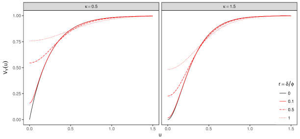
Figure 2.1: Departures (red lines) from the true variogram (solid black line) with $\sigma^{2}=1$ and $\tau^{2}=0$ for increasing values of $r=\delta/\phi$. Matérn correlation functions with two different shape parameters are used.

We now use (2.5) to develop a positional-error-corrected method of variogram-based n-weighted least squares covariance parameter estimation. We assume the positional error variance $\delta^{2}$ to be known, as this is a necessary requirement for identifiability of the model parameters.

Let $\theta$ denote the vector of covariance parameters to be estimated; typically, $\theta=(\tau^{2},\sigma^{2},\phi)$. Write $r_{i}=y_{i}-d(x_{i})^{\top}\tilde{\beta}$, where $\tilde{\beta}$ is a preliminary estimate of $\beta$, for example the ordinary least squares regression estimate, $v_{ij}=\frac{1}{2}(r_{i}-r_{j})^{2}$ and $u_{ij}=\|x_{i}-x_{j}\|$. Our objective function is

$${\cal F}_{n}(\theta)=\stackrel{{\scriptstyle[}}{{\scriptstyle k=1}}]{{\scriptstyle m}}{\sum}n_{k}\{v_{k}-V_{Y}(u_{k};\theta)\}^{2},$$ (2.7)

where: $v_{k}$ are the sample variogram ordinates, obtained by averaging all $v_{ij}$ such $(k-1)h<u_{ij}\leq kh$, where $h$ is the bin width; $u_{k}=(k-0.5)h$ is the mid-point of the corresponding bin interval; $n_{k}$ is the number of pairs $(i,j)$ points that contribute to $v_{k}$; and $V_{Y}(u_{k};\theta)$ is the corrected variogram as defined by (2.5).

3 Likelihood-based inference for the linear Gaussian model

To derive the likelihood function for the linear geostatistical model with positional error, we use the following notation: $Y=(Y_{1},\ldots,Y_{n})$ is the collection of all the random variables associated with our outcome of interest; $S=(S(x_{1}),\ldots,S(x_{n}))$ is the vector of the spatial random effects at the observed locations $x_{i}$ for $i=1,\ldots,n$; $X=\{X_{1},\ldots,X_{n}\}$ and $X^{*}=\{X_{1}^{*},\ldots,X_{n}^{*}\}$ are the perturbed and the true locations, respectively. We then factorize their joint distribution as

$$\left[Y,S,X,X^{*}\right] = \left[Y\mid S,X,X^{*}\right]\left[S,X,X^{*}\right]$$

$$= \left[Y\mid S,X^{*}\right]\left[S\mid X,X^{*}\right]\left[X,X^{*}\right]$$

$$= \left[Y\mid S,X^{*}\right]\left[S\mid X^{*}\right]\left[X^{*}\mid X\right]\left[X\right],$$

where: $\left[Y\mid S,X^{*}\right]=\prod_{i=1}^{n}\left[Y_{i}\mid S(X_{i}^{*})\right]$; $\left[Y_{i}\mid S(X_{i}^{*})\right]$ is Gaussian distribution with mean $S\left(X_{i}^{*}\right)$ and variance $\tau^{2}$; $\left[S\mid X^{*}\right]$ is multivariate Gaussian with mean zero and covariance matrix $\Sigma$ such that $[\Sigma]_{ij}=\sigma^{2}\rho(U^{*}_{ij};\phi,\kappa)$; and $\left[X_{i}^{*}\mid X_{i}\right]$ is a bivariate Gaussian distribution with mean $X_{i}$ and covariance matrix $\delta^{2}I_{2}$. Also, note that in the above equation $\left[Y\mid S,X,X^{*}\right]=\left[Y\mid S,X^{*}\right]$ because of the conditional independence between $Y$ and $X$ given $X^{*}$.

The likelihood function for the unknown vector of parameters $\psi=\left(\beta,\sigma^{2},\phi,\tau^{2}\right)$ is

$$L\left(\psi\right) = \left[Y,X;\psi\right]$$ (3.1)

$$= \int\int\left[Y,X,X^{*},S;\psi\right]dSdX^{*}$$

$$= \int\int\left[Y\mid X,X^{*},S;\psi\right]\left[S,X,X^{*};\psi\right]dSdX^{*}$$

$$= \int\int\left[Y\mid X^{*},S;\psi\right]\left[S\mid X^{*};\psi\right]\left[X^{*}\mid X,\right]\left[X\right]dSdX^{*}$$

$$\propto \int\int\left[Y\mid X^{*},S;\psi\right]\left[S\mid X^{*};\psi\right]\left[X^{*}\mid X\right]dSdX^{*},$$

After integrating out $S$ in (3.1), the final expression for the likelihood is

$$L(\psi)\propto\int\left[Y\mid X^{*}\right]\left[X^{*}\mid X\right]dX^{*},$$ (3.2)

where $\left[Y\mid X^{*},\psi\right]$ is a multivariate Gaussian distribution with mean $D^{*}\beta$ and covariance matrix $\Sigma+\tau^{2}I_{n}$; here, $D^{*}$ denotes the matrix of covariates at the true locations $X^{*}$.

Fanshawe and Diggle, (2011) propose to approximate (3.2) by Monte Carlo integration. Given $\psi$ and $\delta$, they draw $B$ independent samples from $\left[X^{*}\mid X;\psi\right]$. The resulting approximation to the likelihood is then obtained as

$$L(\psi)\approx\frac{1}{B}\left[Y\mid X_{(b)}^{*};\psi\right]$$

where $X_{(b)}^{*}$ is the $b$-th samples from $\left[X^{*}\mid X;\psi\right]$. Maximization of the above expression is computationally intensive since a single evaluation of the approximated likelihood has a computational burden of order $O\left(B\times n^{3}\right)$. For this reason, Fanshawe and Diggle conclude that reliable computation of the standard errors for the maximum likelihood estimates is infeasible.

3.1 Composite likelihood

We propose to approximate the likelihood in (3.2) using the composite likelihood method. The resulting estimating equation obtained from the derivative of the composite log-likelihood is an unbiased estimating equation (Varin et al.,, 2011). This approach has been applied to standard geostatistical models to make computations faster when the number of spatial locations is demanding (Vecchia, 1988; Hjort et al., 1994; Curriero and Lele, 1999; Stein et al., 2004; Caragea and Smith, 2006, 2007; Mateu et al., 2007; Bevilacqua et al., 2012; Bevilacqua and Gaetan, 2015).

The resulting approximation is obtained by treating as independent each of the pairs of bivariate densities, to give

$$\log L(\psi)\approx\log L_{CL}(\psi) = \stackrel{{\scriptstyle[}}{{\scriptscriptstyle i=1}}]{{\scriptscriptstyle n-1}}{\sum}\stackrel{{\scriptstyle[}}{{\scriptscriptstyle j=i+1}}]{{\scriptscriptstyle n}}{\sum}\log[Y_{i},Y_{j};\psi]$$ (3.3)

$$= \stackrel{{\scriptstyle[}}{{\scriptscriptstyle i=1}}]{{\scriptscriptstyle n-1}}{\sum}\stackrel{{\scriptstyle[}}{{\scriptscriptstyle j=i+1}}]{{\scriptscriptstyle n}}{\sum}\log\int_{0}^{\infty}\left[Y_{i},Y_{j}\mid U_{ij}^{*}\right]\left[U_{ij}^{*}\mid u_{ij}\right]dU_{ij}^{*}.$$

Hence, computation of the approximate likelihood requires the integration of $n\left(n-1\right)/2$ univariate integrals. Additionally, note that as the distance between a pair of observations increases, the density function of $[Y_{i},Y_{j}|U_{ij}^{*}]$ tends to

$$[Y_{i}][Y_{j}]=\frac{1}{2\pi\left(\sigma^{2}+\tau^{2}\right)}\exp\left\{-\frac{y_{i}^{2}+y_{j}^{2}}{2\left(\sigma^{2}+\tau^{2}\right)}\right\}.$$

We exploit this fact to further approximate the likelihood function as

$$[Y_{i},Y_{j}|U_{ij}^{*}]\approx[Y_{i},Y_{j}|U_{ij}^{*}]I\left(u_{ij}\leq t\right)+[Y_{i}][Y_{j}]I\left(u_{ij}>t\right),$$ (3.4)

where $I\left(\mathcal{P}\right)$ is an indicator function which takes the value 1 if property $\mathcal{P}$ is verified and 0 otherwise, whilst $t$ is a threshold such that all pairs of observations that are more than a distance $t$ apart are assumed to be independent. Let $U^{*}_{ij,(b)}=Q(s_{b};u_{ij},\delta)$ for $b=1,\ldots,B$, where $Q(\cdot;u_{ij},\delta)$ is the quantile function of a $Rice(u_{ij},\delta)$ and $s_{b}$ is the $b$-th term of a Halton, (1960) sequence.

For $u_{ij}\leq t$, we compute the univariate integral in (3.3) using quasi Monte Carlo methods, i.e.

$$\int_{0}^{\infty}\left[Y_{i},Y_{j}\mid U_{ij}^{*}\right]\left[U_{ij}^{*}\mid u_{ij}\right]dU_{ij}^{*}\approx\frac{1}{B}\sum_{b=1}^{B}[Y_{i},Y_{j}|U^{*}_{ij,(b)}].$$

If $u_{ij}>t$, the integral equals $[Y_{i}][Y_{j}].$

3.2 Uniform geomasking

A commonly used alternative to Gaussian geomasking is uniform geomasking.

Let $W=(W_{1},W_{2})$; we now define the positional error process as

$$\begin{cases}W_{1}=R\cos\Lambda\\ W_{2}=R\sin\Lambda\end{cases},$$ (3.5)

where $R$ and $\Lambda$ are two independent uniform random variables in $[0,\delta]$, with $\delta$ now denoting the maximum displacement distance, and $[0,2\pi]$, respectively. However, note that the resulting distribution of $W$ is not uniform within a disc of radius $\delta$ but has a higher probability density toward the center of the disc. Under uniform geomasking $[U_{ij}^{*}|u_{ij}]$ is an intractable distribution, making computation of the likelihood function in (3.3) cumbersome.

In the application of Section 5, we propose to approximate $[U_{ij}^{*}|u_{ij}]$ under uniform geomasking with a $Rice(u_{ij},\delta/\sqrt{6})$ since the variance for each of the components of $W$ in (3.5) is $\delta^{2}/6$.

We illustrate the quality of this approximation as follows. We first express $U_{ij}^{*}$ in terms of $R$, $\Lambda$ and $u_{ij}$ as

$$U_{ij}^{*}=\sqrt{u_{ij}^{2}+R^{2}-2u_{ij}R\sin\Lambda}.$$ (3.6)

We then simulate 100,000 samples from the uniform distribution on $[0,\delta]$ and 100,000 samples from the uniform distribution on $[0,2\pi]$. For a given value of $u_{ij}$, we then compute the empirical cumulative density function (CDF) of the corresponding 100,000 values generated from $[U_{ij}^{*}|u_{ij}]$, based on (3.6).

Figure 3.1 reports the result of the simulation. The discrepancies between the empirical CDF under uniform geomasking (black line) and the CDF of a $Rice(u_{ij},\delta/\sqrt{6})$ are small in all of the eight scenarios considered. We used values of $\delta=2$ and $\delta=5$ as these correspond to the forms of geomasking that were used in the application of Section 5.

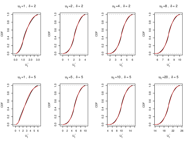
Figure 3.1: Each plot shows the empirical cumulative density function (CDF) based on $100,000$ samples generated from $[U_{ij}^{*}|u_{ij}]$ under uniform geomasking (black line) and the CDF of a $Rice(u_{ij},\delta/\sqrt{6})$ (red line). The corresponding values of $u_{ij}$ and $\delta$ are shown in the heading of each plot.

4 Simulation study

We conducted a simulation study to quantify the effects of positional errors on parameter estimation as follows.

1. Generate $n=1000$ locations $[X^{*}]$ as a homogeneous Poisson process over the square $[0,15]\times[0,15]$.

2. Simulate the outcome data from $[Y|X^{*}]$ as indicated in (2.1), setting $\beta=0$.

3. Simulate from $[X|X^{*}]$ using Gaussian geomasking to obtain $X$.

4. Estimate $\psi$ to obtain $\hat{\psi}_{i}$ for the $i$-th simulated data-set using:

   • variogNaive, a parametric fit to the variogram that ignores using weighted least squares (WLS);

   • variogAdj, a parametric fit to the variogram that corrects for positional error using WLS;

   • geoNaive, maximum likelihood estimation under a linear geostatistical model that ignores positional error;

   • CL, the composite likelihood method of Section 3.1;

   • ACL1, as CL but assuming pairs of observations $Y_{i}$ and $Y_{j}$ to be independent for values of the correlation between $Y_{i}$ and $Y_{j}$ below $0.05$;

   • ACL2, as CL but assuming pairs of observations $Y_{i}$ and $Y_{j}$ to be independent for values of the correlation between $Y_{i}$ and $Y_{j}$ below $0.000005$;

5. Repeat STEPS 1 to 4 $s=500$ times.

6. Calculate the bias,

   $$\frac{1}{s}\sum_{i=1}^{s}\hat{\psi}_{i}-\psi,$$

   and the root-mean-square-error (RMSE),

   $$\sqrt{\frac{1}{s}\sum_{i=1}^{s}\left(\hat{\psi}_{i}-\psi\right)^{2}}.$$

We define the following scenarios: (a) $\sigma^{2}=1$, $\tau^{2}=0$, $\kappa=0.5$ and $\phi=0.25$; (b) $\sigma^{2}=1$, $\tau^{2}=0$, $\kappa=1.5$ and $\phi=0.16$. In both scenarios, we let $r=\delta/\phi$ vary over the set $\{0.2,0.4,0.6,0.8,1\}$. We report the results in Table 1 and 2. As expected, BOTH variogNaive and geoNaive overestimate $\tau^{2}$ and $\phi$ but underestimate $\sigma^{2}$. However, the estimated total variance is not affected by geomasking. In both scenarios, CL shows the smallest RMSE than the other methods for all parameters. The ACL1 and ACL2 show a slight increase in bias and RMSE but with a considerable gain in computational speed. We also observe that the effects of ignoring positional error are less strong on parameter estimation for $\kappa=1.5$ than for $\kappa=0.5$, as the differences in bias and RMSE between the naive and corrected methods are smaller.

Table 1: Bias and root-mean-square-error (RMSE) of the parameter estimates from the naive methods (variogNaive and geoNaive) and those accounting for positional error (variogAdj, CL, ACL1 and ACL2). The true correlation function is Matérn with $\kappa=0.5$.

	$\sigma^{2}$		$\phi$		$\tau^{2}$		$r=\delta/\phi$
Method	Bias	RMSE	Bias	RMSE	Bias	RMSE
variogNaive	-0.106	0.111	0.026	0.036	0.101	0.104	0.2
variogAdj	-0.050	0.069	0.013	0.029	0.014	0.017	0.2
geoNaive	-0.166	0.196	0.037	0.039	0.149	0.179	0.2
CL	-0.053	0.069	-0.001	0.017	0.015	0.016	0.2
ACL2	-0.053	0.069	-0.001	0.017	0.015	0.016	0.2
ACL1	-0.052	0.068	0.005	0.021	0.015	0.016	0.2
variogNaive	-0.266	0.327	0.070	0.120	0.279	0.319	0.4
variogAdj	-0.053	0.072	0.013	0.035	0.002	0.002	0.4
geoNaive	-0.323	0.421	0.083	0.124	0.321	0.410	0.4
CL	-0.052	0.071	-0.002	0.018	0.002	0.002	0.4
ACL2	-0.052	0.071	-0.002	0.018	0.002	0.001	0.4
ACL1	-0.051	0.071	0.003	0.025	0.002	0.002	0.4
variogNaive	-0.410	0.412	0.158	0.160	0.444	0.453	0.6
variogAdj	-0.055	0.072	0.024	0.041	0.007	0.011	0.6
geoNaive	-0.458	0.466	0.138	0.142	0.456	0.458	0.6
CL	-0.057	0.071	0.000	0.022	0.009	0.010	0.6
ACL2	-0.057	0.071	0.000	0.022	0.009	0.010	0.6
ACL1	-0.057	0.072	0.010	0.028	0.009	0.011	0.6
variogNaive	-0.519	0.522	0.268	0.271	0.574	0.579	0.8
variogAdj	-0.067	0.092	0.037	0.049	0.030	0.041	0.8
geoNaive	-0.571	0.577	0.187	0.195	0.566	0.580	0.8
CL	-0.063	0.080	-0.004	0.025	0.038	0.039	0.8
ACL2	-0.063	0.080	-0.004	0.025	0.038	0.039	0.8
ACL1	-0.063	0.079	0.009	0.035	0.032	0.033	0.8
variogNaive	-0.587	0.603	0.437	0.444	0.667	0.675	1.0
variogAdj	-0.066	0.097	0.051	0.060	0.023	0.030	1.0
geoNaive	-0.655	0.663	0.243	0.251	0.653	0.660	1.0
CL	-0.071	0.088	-0.007	0.035	0.027	0.029	1.0
ACL2	-0.071	0.088	-0.008	0.031	0.025	0.028	1.0
ACL1	-0.071	0.088	0.009	0.044	0.023	0.027	1.0

Table 2: Bias and root-mean-square-error (RMSE) of the parameter estimates from the naive methods (variogNaive and geoNaive) and those accounting for positional error (variogAdj, CL, ACL1 and ACL2). The true correlation function is Matérn with $\kappa=1.5$.

	$\sigma^{2}$		$\phi$		$\tau^{2}$		$r=\delta/\phi$
Method	Bias	RMSE	Bias	RMSE	Bias	RMSE
variogNaive	-0.049	0.095	0.009	0.023	0.051	0.073	0.2
variogAdj	-0.033	0.086	0.007	0.022	0.034	0.059	0.2
geoNaive	-0.053	0.079	0.008	0.012	0.048	0.051	0.2
CL	-0.038	0.084	0.000	0.011	0.035	0.059	0.2
ACL2	-0.038	0.084	0.000	0.011	0.035	0.059	0.2
ACL1	-0.038	0.085	0.002	0.012	0.035	0.060	0.2
variogNaive	-0.124	0.154	0.018	0.030	0.124	0.141	0.4
variogAdj	-0.050	0.102	0.008	0.024	0.049	0.079	0.4
geoNaive	-0.147	0.160	0.020	0.024	0.141	0.145	0.4
CL	-0.052	0.099	0.001	0.011	0.049	0.078	0.4
ACL2	-0.052	0.099	0.001	0.011	0.049	0.078	0.4
ACL1	-0.053	0.101	0.002	0.014	0.050	0.081	0.4
variogNaive	-0.212	0.230	0.031	0.044	0.217	0.228	0.6
variogAdj	-0.048	0.105	0.009	0.030	0.050	0.092	0.6
geoNaive	-0.243	0.252	0.035	0.039	0.240	0.244	0.6
CL	-0.051	0.104	0.000	0.013	0.049	0.086	0.6
ACL2	-0.051	0.105	0.000	0.013	0.049	0.087	0.6
ACL1	-0.052	0.107	0.002	0.019	0.050	0.090	0.6
variogNaive	-0.312	0.324	0.051	0.061	0.325	0.332	0.8
variogAdj	-0.059	0.118	0.013	0.032	0.066	0.114	0.8
geoNaive	-0.345	0.352	0.054	0.058	0.345	0.349	0.8
CL	-0.063	0.119	0.001	0.014	0.063	0.106	0.8
ACL2	-0.063	0.119	0.001	0.014	0.063	0.106	0.8
ACL1	-0.065	0.125	0.004	0.020	0.065	0.112	0.8
variogNaive	-0.400	0.408	0.079	0.090	0.420	0.426	1.0
variogAdj	-0.076	0.146	0.022	0.042	0.088	0.145	1.0
geoNaive	-0.433	0.438	0.074	0.078	0.433	0.435	1.0
CL	-0.082	0.144	0.001	0.021	0.083	0.134	1.0
ACL2	-0.083	0.145	0.001	0.029	0.083	0.135	1.0
ACL1	-0.086	0.152	0.006	0.022	0.087	0.148	1.0

5 Application

We analyse data on children’s height-for-age Z-scores (HAZs) from a Demographic and Health Survey (Burgert et al.,, 2013) conducted in Senegal in 2011. HAZs are a measure of the deviation from standard growth as defined by the WHO Growth Standards (deOnis2007) and are comparable across age and gender. A value of HAZ below -2 indicates stunted growth.

In this survey, the sampling unit are clusters of households within a predefined geographic area known as a census enumeration area (EA). An EA typically corresponds to a single city block or apartment building in urban areas and to a village or group of villages in rural areas The estimated centre of each cluster is recorded as a latitude/longitude coordinate, obtained from a GPS receiver or derived from public online maps or gazetteers (Gething et al.,, 2015). To preserve the confidentiality of survey respondents, uniform geomasking was applied to the cluster centres. To take into account the different population density, different values for the maximum displacement distance were applied to urban and rural locations, specifically $\delta_{urbarn}=2$ km and $\delta_{rural}=5$ km.

The data consist of 384 clusters, of which 122 are urban, with 10 children per cluster on average. Our outcome of interest, $Y_{i}$, is the average HAZ for a cluster which we model as

$$Y_{i}=\mu+S(x_{i})+Z_{i}$$ (5.1)

where $Z_{i}\sim N(0,\tau^{2}/n_{i})$ and $n_{i}$ is the number of children at the $i$-th cluster. To account for positional error, we approximate uniform geomasking with its Gaussian counterpart as explained in Section 3.2.

Table 3 reports the parameter estimates from the naive geostatistical model (first row) and the proposed modelling approach (second row). We were not able to obtain reliable estimates from the variogram-based correction approach due to the relatively high noise to signal ratio. As in simulation study, the naive geostatistical model approach yields a larger point estimates for $\tau^{2}$ and $\phi$ but smaller for $\sigma^{2}$. The point estimates for the practical range as estimated from for the naive model and from the model that accounts for the geomasking are $133.81$ km and $77.47$ km, respectively.

We also note that accounting for positional error also leads to narrower confidence intervals for all the model parameters expect the mean $\mu$.

Table 3: Parameter estimates and corresponding 95$\%$ confidence intervals (CI) for the fitted linear geostatistical models to malnutrition data of Section 5. “geoNaive” is the naive approach which ignores positional error, while “CL” is the proposed approach based on the composite likelihood.

	geoNaive		CL
Parameter	Estimate	95$\%$ CI	Estimate	95$\%$ CI
$\mu$	-1.303	(-1.470, -1.137)	-1.159	(-1.562, -0.736)
$\sigma^{2}$	0.117	(0.045, 0.289)	0.197	(0.146, 0.257)
$\phi$	44.669	(9.184, 80.138)	25.860	(17.782, 37.614)
$\tau^{2}$	0.536	(0.081, 0.994)	0.464	(0.409, 0.521)

6 Discussion

We have developed a computationally efficient approximation for maximum likelihood estimation of the linear geostatistical model under geomasking using the composite likelihood (CL) method. We have compared the performance of this approach with standard geostatistical approaches that ignore positional error and with a corrected variogram-based parametric fit. The CL method outperformed both, leading to substantially smaller root-mean-square-errors for the parameter estimates. The CL method also provides a computationally more efficient alternative to Fanshawe and Diggle, (2011) by reducing the computational burden from $O\left(B\times n^{3}\right)$, where $B$ is the number of Monte Carlo simulations, to $O\left(n^{2}\right)$. Our results indicate that ignoring positional error due to geomasking can lead to an overestimation of the nugget effect variance and the scale of the spatial correlation, while underestimating the variance of the residual spatial random effects.

The effects of geomasking on parameter estimation are stronger for larger values in the ratio $r=\delta/\phi$, where $\delta$ is the standard deviation of the positional error process in the case of Gaussian geomasking or the maximum displacement distance under uniform geomasking, $\phi$ is the scale of the spatial correlation. For this reason, geomasking procedures should always use the smallest acceptable value for $r$. High values of $r$ weaken the structure of the spatial dependence in the data, thus leading to less accurate predictive inferences.

In the application of Section 5, we approximated uniform geomasking with its Gaussian counterpart. As shown in Section 3.2, the discrepancies between the true cumulative density function (CDF) of $[U_{ij}^{*}|u_{ij}]$ under uniform geomasking and the CDF of the Rice distribution that we used as an approximation are small in this case. Future research will investigate the robustness of this approach more generally under different scenarios.

Appendix A Appendix

A.1 Rice distribution

The random variable $U$ follows a $Rice(\nu,\sigma)$ if its density function is

$$f\left(u;\nu,\sigma\right)=\frac{u}{\sigma^{2}}\exp\left(-\frac{u^{2}+\nu^{2}}{2\sigma^{2}}\right)I_{0}\left(\frac{u\nu}{\sigma^{2}}\right),$$

with $I_{k}\left(\cdot\right)$ is the modified Bessel function of the first kind with order $k$.

The mean of $U$ is

$$E[U]=\sigma\sqrt{\frac{\pi}{2}}L(\nu^{2}/2\sigma^{2})$$

where

$$L(x)=e^{x/2}\left[(1-x)I_{0}(x/2)-xI_{1}(x/2)\right];$$

the variance is

$$\text{Var}[U]=2\sigma^{2}+\nu^{2}-\frac{\pi\sigma^{2}}{2}L^{2}(-\nu^{2}/2\sigma^{2}).$$

A Rice variable is also obtained as

$$U=\sqrt{X_{1}^{2}+X_{2}^{2}},$$

where $X_{1}$ and $X_{2}$ are independent Gaussian variables both with variance $\sigma^{2}$, and mean $\nu\cos\theta$ and $\nu\sin\theta$, respectively.

References

- Arbia et al., (2015) Arbia, G., Espa, G., and Giuliani, D. (2015). Dirty spatial econometrics. Ann. Reg. Sci., 56(1):177–189.
- Armstrong et al., (1999) Armstrong, M. P., Rushton, G., and Zimmerman, D. L. (1999). Geographically masking health data to preserve confidentiality. Stat. Med., 18(5):497–525.
- Bevilacqua and Gaetan, (2015) Bevilacqua, M. and Gaetan, C. (2015). Comparing composite likelihood methods based on pairs for spatial gaussian random fields. Stat. Comput., 25(5):877–892.
- Bevilacqua et al., (2012) Bevilacqua, M., Gaetan, C., Mateu, J., and Porcu, E. (2012). Estimating space and Space-Time covariance functions for large data sets: A weighted composite likelihood approach. J. Am. Stat. Assoc., 107(497):268–280.
- Bonner et al., (2003) Bonner, M. R., Han, D., Nie, J., Rogerson, P., Vena, J. E., and Freudenheim, J. L. (2003). Positional accuracy of geocoded addresses in epidemiologic research. Epidemiology, 14(4):408–412.
- Burgert et al., (2013) Burgert, C. R., Colston, J., Roy, T., and Zachary, B. (2013). Geographic displacement procedure and georeferenced data release policy for the demographic and health surveys.
- Caragea and Smith, (2006) Caragea, P. and Smith, R. L. (2006). Approximate likelihoods for spatial processes. Preprint.
- Caragea and Smith, (2007) Caragea, P. C. and Smith, R. L. (2007). Asymptotic properties of computationally efficient alternative estimators for a class of multivariate normal models. J. Multivar. Anal., 98(7):1417–1440.
- Cassa et al., (2006) Cassa, C. A., Grannis, S. J., Overhage, J. M., and Mandl, K. D. (2006). A context-sensitive approach to anonymizing spatial surveillance data: impact on outbreak detection. J. Am. Med. Inform. Assoc., 13(2):160–165.
- Cayo and Talbot, (2003) Cayo, M. R. and Talbot, T. O. (2003). Positional error in automated geocoding of residential addresses. Int. J. Health Geogr., 2(1):10.
- Cressie and Kornak, (2003) Cressie, N. and Kornak, J. (2003). Spatial statistics in the presence of location error with an application to remote sensing of the environment. Stat. Sci., pages 436–456.
- Curriero and Lele, (1999) Curriero, F. C. and Lele, S. (1999). A composite likelihood approach to semivariogram estimation. J. Agric. Biol. Environ. Stat., 4(1):9–28.
- Dearwent et al., (2001) Dearwent, S. M., Jacobs, R. R., and Halbert, J. B. (2001). Locational uncertainty in georeferencing public health datasets. J. Expo. Anal. Environ. Epidemiol., 11(4):329–334.
- Devillers and Jeansoulin, (2006) Devillers, R. and Jeansoulin, R. (2006). Fundamentals of spatial data quality. ISTE Publishing Company.
- Diggle and Ribeiro, (2007) Diggle, P. and Ribeiro, P. J. (2007). Model-based Geostatistics. Springer.