Nonlinear quantum Langevin equations for bosonic modes in solid-state systems

Abstract

Based on the experimental evidence that impurities contribute to the dissipation properties of solid-state open quantum systems, we provide here a description in terms of nonlinear quantum Langevin equations of the role played by two-level systems in the dynamics of a bosonic degree of freedom. Our starting point is represented by the description of the system/environment coupling in terms of coupling to two separate reservoirs, modelling the interaction with external bosonic modes and two level systems, respectively. Furthermore, we show how this model represents a specific example of a class of open quantum systems that can be described by nonlinear quantum Langevin equations. Our analysis offers a potential explanation of the parametric effects recently observed in circuit-QED cavity optomechanics experiments.

The dynamics of open quantum systems –i.e. quantum systems that can be described as separate entities from their surrounding environment while being somehow coupled to it– is arguably one of the most fundamental problems in quantum mechanics, encompassing concepts such as the measurement paradox Leggett (2005), and the boundary between quantum and classical physics Zurek (1991). On general grounds, the interaction between a quantum system and its environment represents an important aspect of the physics of condensed matter and complex systems, which has been the focus of extensive analysis Leggett et al. (1987); Breuer and Petruccione (2007); Breuer et al. (2016), with repercussions in contexts ranging from the energy transport in photosynthetic complexes Ishizaki et al. (2010) to the physics of ultracold gases Leskinen et al. (2010); Massel et al. (2013); Visuri et al. (2014).

In the description of these systems the inclusion of the role played by coupling to an external environment is necessary, if only because the system has to be coupled to an external measurement apparatus which, from the quantum-dynamical perspective of the system, represents a source of noise and dissipation. At the same time the manipulation of open quantum systems has recently led to the possibility of preparing and detecting quantum states of matter and radiation Ano (2012); Wiseman and Milburn (2010), paving the way for the definition of a new paradigm of quantum technology which represents an important field for applications ranging from secure (quantum) communication Nielsen and Chuang (2010) to sensing of electromagnetic fields Clerk et al. (2010) and to the detection of gravitational waves Abbott et al. (2016). This prospect of technological application of quantum mechanics is rooted in the relatively recent development of fabrication techniques at the nanoscale, in particular nanomechanical resonators, superconducting qubits and, more in general, circuit quantum electrodynamics (QED) setups Wallraff et al. (2004); Sillanpää et al. (2007); Majer et al. (2007); Schoelkopf and Girvin (2008) where the characteristic scales involved in the dynamics of these systems naturally lead to the study of the quantum properties in the presence of coupling to an environment.

Within this framework, it has recently been observed that this coupling can represent an important resource leading to the notion of reservoir engineering Poyatos et al. (1996). This concept corresponds to the idea that, by manipulating the properties of the environment coupled to a given quantum system or even the nature of the system environment coupling itself, it is possible to generate specific (quantum) states for the system. Prominent examples are represented by the recent achievements in the field of cavity optomechanics, where ground state cooling Teufel et al. (2011) and squeezing below the standard quantum limit (SQL) Wollman et al. (2015); Pirkkalainen et al. (2015); Lecocq et al. (2015), along with nearly quantum limited amplification Massel et al. (2011); Ockeloen-Korppi et al. (2016) and nonreciprocal photon transmission Metelmann and Clerk (2015) have been achieved by introducing a specific (Gaussian) state for the reservoir. While these examples correspond to inducing a specific state for the system by manipulating the state of the reservoir, in Refs. Mirrahimi et al. (2014); Leghtas et al. (2015) it is shown that, by designing a specific nonlinear coupling between system and environment: it is possible to protect certain quantum states (cat states) against decoherence.

If the coupling between the system and the environment is described by a linear Hamiltonian, the effects of noise and dissipation on the dynamics of the system can be described in terms of linear quantum Langevin equations (QLEs) Wiseman and Milburn (2010). These equations represent an extension to the quantum regime of the classical Langevin equations and, in analogy to their classical counterpart, include in the description of the dynamics of the system the role played by the environment, including dissipative and noise effects. However the case of a linear system/environment coupling is not the most general situation that can arise: for instance, for nanomechanical resonators Zolfagharkhani et al. (2005); Arcizet et al. (2009); Eichler et al. (2011); Suh et al. (2012); Singh et al. (2016) and for circuit QED setups Simmonds et al. (2004); Martinis et al. (2005); Ashhab et al. (2006); O’Connell et al. (2008); Gao et al. (2008); Neill et al. (2013), the experimental evidence of nonlinear phenomena related to the coupling between system and environment has emerged and, more importantly for our analysis, the relevance of impurities in this phenomenon has been discussed. In both setups, it has been shown that the impurities, naturally arising in the material composing the devices, its supports and/or substrate, represent a source of dissipation. These defects can be modelled in terms of TLSs. The reason behind the possibility of modelling impurities in these terms is represented by the fact that each impurity can be construed as quantum systems which exhibit two local energy minima. For instance as a charged impurity that can hop between two defects in the crystal structure, or a dangling bond with two possible configurations.

More specifically, these TLSs exist primarily due to the disordered potential landscape of amorphous materials – e.g. in surface oxides of thin-film circuit electrodes Gao et al. (2008), in the tunnel barrier of Josephson junctions Simmonds et al. (2004), and at disordered interfaces Phillips (1987); Quintana et al. (2014) – coupling with the bosonic degrees of freedom of the system, either through a purely electromagnetic interaction (optical and circuit QED setups) or a phononic one in the context of nanomechanical systems Kleiman et al. (1987).

In this Letter we show under what conditions, considering a nonlinear coupling between system and a bath of TLSs, it is possible to derive a nonlinear a QLE for the dynamics of the degrees of freedom of the system, having in mind a circuit QED setup. In addition, we show how the nonlinear QLEs derived here can represent an explanation to some of the phenomena recently observed in the context of microwave quantum optomechanics Pirkkalainen et al. (2015).

The starting point for our analysis is represented by a bosonic system $(\mathcal{S})$ coupled to an environment $(\mathcal{E})$ . The total Hamiltonian of the bipartite system $(\mathcal{S}+\mathcal{E})$ is given by

$$H=H_{\mathcal{S}}+H_{\mathcal{E}}+H_{\mathcal{S}-\mathcal{E}},$$ (1)

where $H_{\mathcal{S}}=H_{\mathcal{S}}(c,c^{\dagger})$ is the Hamiltonian of the isolated system, exhibiting a generic dependence on the annihilation (creation) operators $c$ $(c^{\dagger})$ associated with the system, and $H_{\mathcal{E}}$ is the Hamiltonian for the bath.

We assume here that the environment Hamiltonian can be decomposed into two terms, $H_{\mathcal{E}}^{\mathrm{B}}=\sum_{\mathrm{k}}\omega_{\mathrm{k}}b^{\dagger}_{\mathrm{k}}b_{\mathrm{k}}$ and $H_{\mathcal{E}}^{\mathrm{TLS}}$, corresponding to a bath of free bosonic modes, and to a bath of TLSs, respectively. The bosonic bath describes, for instance, the modes of the electromagnetic field of the environment. In our analysis we assume that these modes, while being associated with the noise properties and dissipation of the system, encompass also the external coherent fields driving the system whose properties are encoded in the state of the bath for the modes $b_{\mathrm{k}}$. Our choice is equivalent to considering a coherent driving term for the system Hamiltonian and a purely thermal bath.

In this scenario, we describe the coupling between these modes and the degrees of freedom of the system by the following Hamiltonian

$$H_{\mathcal{\mathcal{S}-\mathrm{B}}}=\sum g_{\mathrm{k}}^{\mathrm{B}}\left(c^{\dagger}b_{\mathrm{k}}+cb^{\dagger}_{\mathrm{k}}\right).$$ (2)

In addition, we model the bath of TLSs as a collection of spins $\mathbf{J}_{\mathrm{k}}$. In this scenario we have that $H_{\mathcal{E}}^{\mathrm{TLS}}=\sum\Omega_{\mathrm{k}}J_{z}^{\mathrm{k}}$. This choice for the modeling of TLSs corresponds to the idea that, for each $\Omega_{\mathrm{k}}$ multiple TLSs are present that collectively couple with the system $\mathcal{S}$. While for $\Omega_{\mathrm{k}}\simeq\omega_{\mathrm{S}}$ –where $\omega_{\mathrm{S}}$ corresponds to a characteristic frequency for the system– the presence of impurities leads to a renormalization of the linewidth associated with the linear response of the system induced by the coupling given in Eq. (2) (see Appendix D); for $\Omega_{\mathrm{k}}\simeq n\,\omega_{\mathrm{S}}$, nonlinear contributions appear. In our analysis, also in light of the recent investigations concerning the relevance of two-photon emission processes by TLSs Lindkvist and Johansson (2014); Fischer et al. (2017) when coupled to bosonic modes, we consider the case $n=2$, representing the lowest-order approximation beyond linear coupling.

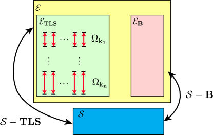
Figure 1: Cartoon picture of the setup. The system $\mathcal{S}$ is coupled to an environment $\mathcal{E}$, which is constituted by a bosonic bath $\mathcal{E}_{\mathrm{B}}$ and a bath of TLSs $\mathcal{E}_{\mathrm{TLS}}$. The coupling between the two baths and the system is mediated by the Hamiltonians $H_{\mathcal{S}-\mathrm{B}}$ and $H_{\mathcal{S}-\mathrm{TLS}}$,respectively.

This assumption appears to be compatible with the usual experimental conditions encountered in the context of circuit QED where microwave cavities operate at frequencies corresponding to few GHz Wallraff et al. (2004); Sillanpää et al. (2007); Grabovskij et al. (2012) while the energy separation of a TLS relevant for the physics of either of these systems is of the order of $10\,$GHz Grabovskij et al. (2012); Holder et al. (2013). In this case, it is possible to write the system-TLS coupling Hamiltonian as

$$H_{\mathcal{S}-\mathrm{TLS}} =\sum_{\mathrm{k}}g^{\mathrm{TLS}}_{\mathrm{k}}\left(J^{\mathrm{k}}_{+}c^{2}+J^{\mathrm{k}}_{-}{c^{\dagger}}^{2}\right).$$ (3)

If we assume that $\left|\mathbf{J}_{\mathrm{k}}\right|\gg 1$, corresponding to the idea that, for each value of $\mathrm{k}$ multiple TLSs couple to the system $\mathcal{S}$, by resorting to the Holstein-Primakoff (HP) realization of spin operators in terms of bosonic modes, we can replace the spin operators with bosonic ones. This mapping can be performed in two different ways, corresponding to complementary experimental conditions (see Appendix A) . If it is assumed that the TLSs mostly reside in their ground state, we have that $J^{\mathrm{k}}_{3}\simeq-j_{\mathrm{k}}$ – where $j_{\mathrm{k}}$ is the index of the representation associated with the spin $\mathbf{J}_{\mathrm{k}}$– and the HP mapping reads $J^{\mathrm{k}}_{3}\to d^{\dagger}_{\mathrm{k}}d_{\mathrm{k}}-j_{\mathrm{k}}$, $J^{\mathrm{k}}_{-}\to d_{\mathrm{k}}$, $J^{\mathrm{k}}_{+}\to d_{\mathrm{k}}^{\dagger}$. In this case, the coupling between the system and the TLS bath can be approximated by

$$H_{\mathcal{S}-\mathrm{HP}_{-}} =\sum_{\mathrm{k}}g^{\mathrm{HP}}_{\mathrm{k}}\left(d_{\mathrm{k}}^{\dagger}c^{2}+d_{\mathrm{k}}{c^{\dagger}}^{2}\right).$$ (4)

with $g^{\mathrm{HP}}_{\mathrm{k}}=\sqrt{2j_{\mathrm{k}}}g^{\mathrm{TLS}}_{\mathrm{k}}$ On the other hand, if the TLSs mainly reside in their excited state ($J^{\mathrm{k}}_{3}\simeq+j$) the mapping can be written as $J^{\mathrm{k}}_{3}\to j_{\mathrm{k}}-d^{\dagger}_{\mathrm{k}}d_{\mathrm{k}}$, $J^{\mathrm{k}}_{-}\to d^{\dagger}_{\mathrm{k}}$, $J^{\mathrm{k}}_{+}\to d_{\mathrm{k}}$, leading to the following approximation for $H_{\mathcal{S}-\mathrm{TLS}}$

$$H_{\mathcal{S}-\mathrm{HP}_{+}} =\sum_{\mathrm{k}}g^{\mathrm{TLS}}_{\mathrm{k}}\left(d_{\mathrm{k}}c^{2}+d_{\mathrm{k}}^{\dagger}{c^{\dagger}}^{2}\right).$$ (5)

These two different forms of the HP mapping correspond to two different physical situations: in the former case, the TLSs prevalently reside in their ground state corresponding to the idea that the impurities mainly reside in their ground state, implying a low-temperature regime. In this case, the bosonic excitations described by the operators $d_{\mathrm{k}}$, represent (weak) excitations around the ground state. On the other hand, the latter case corresponds to the situation in which the highest-excited (metastable) state of the TLSs is weakly (de-)excited: corresponding, for instance, to the case in which an external drive induces excitations in the TLSs bath, leading to a possible interpretation of the linewidth narrowing observed in circuit QED setups under strong driving conditions Martinis et al. (2005) in terms of nonlinear QLEs associated with the saturation of the TLSs. In this picture, the external drive effectively heats the impurities to their excited state, inducing the population inversion for the ensemble of TLSs and a consequent saturation, justifying the $HP_{+}$ transformation in terms of (weak) de-excitations of the highest-excited state.

As we show in Appendix B, it is possible to derive QLEs for the system, provided that the environment Hamiltonian is described by a set of bosonic operators, coupled linearly to the system degrees of freedom. It is important to note that the requirement of linearity concerning the system/environment Hamiltonian is limited to the bath degrees of freedom, meaning that its most general form can be expressed as

$$H_{\mathcal{S}-\mathcal{E}}=\sum_{\mathrm{k}}g_{\mathrm{k}}\left[F^{\dagger}\left(c,c^{\dagger}\right)e_{\mathrm{k}}+F\left(c,c^{\dagger}\right)e_{\mathrm{k}}^{\dagger}\right],$$ (6)

where $e_{\mathrm{k}}$ and $e^{\dagger}_{\mathrm{k}}$ represent generic bosonic operators associated with the environment degrees of freedom. The form the system/environment coupling represents a sufficient condition for the derivation of a nonlinear QLE, along with the assumption that the modes of the bath are noninteracting. In other terms, it is necessary to assume a linear dependence of the coupling Hamiltonian on the environment degrees of freedom since, in order to derive the QLEs for the system, the solution of the Heisenberg equation of motion for the environment degrees of freedom has to assume a specific form, in which the contribution of the system and the environment operators can be represented as two separate additive terms (see Appendix B) .

It is therefore clear that, since the form of $H_{\mathcal{S}-\mathrm{B}}$ and $H_{\mathcal{S}-\mathrm{HP}_{\pm}}$ can be expressed in the form given by Eq. (6), with $F\left(c,c^{\dagger}\right)$ given by $c$, $c^{2}$ and ${c^{\dagger}}^{2}$, and with $e_{\mathrm{k}}=b_{\mathrm{k}}$ and $e_{\mathrm{k}}=d_{\mathrm{k}}$ for $\mathcal{S}-\mathrm{B}$, $\mathcal{S}-\mathrm{HP}_{-}$,$\mathcal{S}-\mathrm{HP}_{+}$ respectively, we can write the dynamics of the system in terms of a (nonlinear) QLE as

$$\dot{c}=-i\left[c,H_{\mathcal{S}}\right] -\left(\frac{\kappa}{2}+\kappa_{N}c^{\dagger}c\right)c$$

$$+\sqrt{\kappa}c_{\mathrm{in}}+2\sqrt{\kappa_{N}}c^{\dagger}c^{\mathrm{TLS}}_{\mathrm{in}}$$ (7a)

$$\dot{c}=-i\left[c,H_{\mathcal{S}}\right] -\left(\frac{\kappa}{2}-\kappa_{N}c^{\dagger}c\right)c$$

$$+\sqrt{\kappa}c_{\mathrm{in}}+2\sqrt{\kappa_{N}}c^{\dagger}{c_{\mathrm{in}}^{\mathrm{TLS}}}^{\dagger}.$$ (7b)

Eqs. (7a,7b), obtained considering the system/environment coupling given by $H_{\mathcal{S}-\mathrm{HP}_{-}}$ and $H_{\mathcal{S}-\mathrm{HP}_{+}}$ respectively, are the main result of our analysis: the presence of a TLS bath leads to the appearance of nonlinear dissipative terms ($\pm\kappa_{\mathrm{N}}c^{\dagger}c\,c$), and to purely imaginary parametric noise terms ($2\sqrt{\kappa_{\rm N}}c^{\dagger}{c_{\rm in}^{\rm TLS}}^{(\dagger)}$). We stress here that these terms are the direct result of the modelling of the bath in terms of two-separate environments ($H_{\mathcal{S}-\mathrm{B}}$ and $H_{\mathcal{S}}-\mathrm{HP_{\pm}}$), and do not represent an ad-hoc modification of the linear QLEs that can be derived in the absence of coupling to TLSs. In particular, while the nonlinear dissipation term possibly represents a natural extension to the nonlinear regime of linear QLEs, the parametric noise term is a nontrivial contribution associated with the presence of the TLS bath.

In addition we observe here that, analogously to their linear counterpart, Eqs. (7b) are time-local, i.e. the dynamics is Markovian. As detailed in Appendix B, this property is related to the assumption that, within the range of frequencies of interest, the coupling strength between system and environment is independent of the mode considered (wide band limit approximation) Stefanucci and van Leeuwen (2014).

If we further consider a pump-probe representative of a circuit QED setup (e.g. a circuit optomechanical experiment), we can assume that the dynamics given by Eq. (8b) is linearized around a strong coherent tone

$$\alpha_{\mathrm{p}}=\alpha_{\mathrm{in}}\exp\left[-i\omega_{\mathrm{p}}t\right].$$

The frequency $\omega_{\mathrm{p}}$ is detuned by $\Delta=\omega_{\mathrm{p}}-\omega_{\mathrm{c}}$ from the cavity resonant frequency. As a result of the linearization scheme, we have that the amplitude of the cavity field oscillating at $\omega_{\mathrm{p}}$ is given by the solution of a nonlinear algebraic equation. In Fig. 2 we have plotted the stationary value of the cavity field for the two choices of the HP mapping ($\mathrm{HP}_{\pm}$). As expected, for small values of the driving field $\alpha_{\mathrm{in}}$, the stationary solution corresponds to the solution in the absence of nonlinear dissipation. However, for larger values of $\alpha_{\mathrm{in}}$ the stationary solution substantially deviates from the solution of the linear system, with, for the parameters discussed here, a negligible difference between $\mathrm{HP}_{\pm}$ cases.

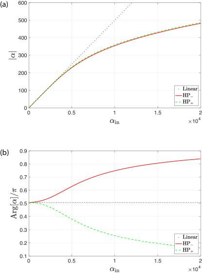
Figure 2: Amplitude (a) and phase (b), for the stationary value (in a frame rotating at $\omega_{\mathrm{p}}$, see text) of the cavity field $\alpha$ in the presence of a driving $\alpha_{\mathrm{in}}$. Parameters: $\kappa_{\mathrm{N}}=1.5\times 10^{-4}$, $\Delta=20$ (all quantities are expressed in units of $\kappa$).

Furthermore, the (first-order) dynamics of the fluctuations $c=\alpha+a$ around the stationary value induced by the pump (in a frame rotating at $\omega_{\mathrm{p}}$) is given by

$$\dot{a}= \left[i\Delta-\left(\frac{\kappa}{2}+2\kappa_{N}\left|\alpha\right|^{2}\right)\right]a-\kappa_{N}\alpha^{2}a^{\dagger}$$

$$+\sqrt{\kappa}a_{\mathrm{in}}+2\sqrt{\kappa_{N}}\alpha^{*}a^{\mathrm{TLS}}_{\mathrm{in}}$$ (8a)

$$\dot{a}= \left[i\Delta-\left(\frac{\kappa}{2}-2\kappa_{N}\left|\alpha\right|^{2}\right)\right]a+\kappa_{N}\alpha^{2}a^{\dagger}$$

$$+\sqrt{\kappa}a_{\mathrm{in}}+2\sqrt{\kappa_{N}}\alpha^{*}{a_{\mathrm{in}}^{\mathrm{TLS}}}^{\dagger}$$ (8b)

$\mathrm{HP}_{-}$ and $\mathrm{HP}_{+}$ case respectively (see Appendix C). It is possible to see that Eqs. (8a,8b) include a purely imaginary parametric term, on top of a nonlinear dissipation term implying linewidth broadening or narrowing, depending on the state of the TLSs bath. Recently, in Ref. Pirkkalainen et al. (2015) a term of the same form was introduced as an ad-hoc parameter, in order to match the experimental results of a cavity optomechanical experiment aimed at establishing squeezing below the SQL of a nanomechanical resonator.

Our description, therefore provides a potential explanation of such parametric effects in terms of nonlinear dissipation phenomena associated with the nonlinear coupling to a bath of TLSs. In order to characterize the effect induced by the presence of the nonlinear coupling to TLSs, we evaluate the fluctuation spectrum of the cavity field $S_{\omega}^{\theta}=1/2\langle\left\{X^{\theta}_{\omega},X^{\theta}_{-\omega}\right\}\rangle$ – with $X_{\omega}^{\theta}=1/\sqrt{2}\left(a_{-\omega}^{\dagger}e^{i\theta}+a_{\omega}e^{-i\theta}\right)$ – assuming thermal fluctuations both for the bosonic and the TLS bath. As hinted by the structure of Eqs. (8a,8b), the presence of a parametric term induces squeezing, which can be experimentally observed by homodyne detection of the output field, in the cavity spectrum for both cases, as it is possible to see from Fig. 3 where it is possible to see how the cavity fluctuation spectrum exhibits a clear dependence on the phase $\theta$.

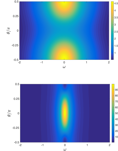
Figure 3: Noise spectrum for the cavity field in the presence of an external drive $\alpha_{\mathrm{in}}=700$, for (a) $\mathrm{HP}_{-}$ and (b) $\mathrm{HP}_{+}$ for $\langle a^{\dagger}_{\mathrm{in}}a_{\mathrm{in}}\rangle=\langle{a_{\mathrm{in}}^{\mathrm{TLS}}}^{\dagger}a^{\mathrm{TLS}}_{\mathrm{in}}\rangle=1$ (all other parameters as in Fig. 2).

We have reported here how it is possible to deduce nonlinear QLEs for the dynamics of an open quantum system from a nonlinear system/environment coupling Hamiltonian. Moreover, we have discussed how an effective nonlinear system/environment coupling can emerge in the presence of impurities modeled as TLSs. Ultimately, we have shown that the TLS-induced nonlinearities can represent a potential explanation for the imaginary parametric terms reported in Ref. Pirkkalainen et al. (2015).

This work was supported by the Academy of Finland (Contract No. 275245).

Appendix A Holstein-Primakoff transformation

We discuss here the Holstein-Primakoff realization allowing us to replace the spin operators $J_{z}$, $J_{\pm}$ obeying the usual SU(2) commutation relations

$$\left[J_{z}^{\mathrm{k}},J_{\pm}^{\mathrm{k}}\right]=\pm J_{\pm}^{\mathrm{k}},\qquad\left[J_{+}^{\mathrm{k}},J_{-}^{\mathrm{k}}\right]=2J_{z}^{\mathrm{k}},$$ (9)

with bosonic operators $d_{\mathrm{k}}$, $d_{\mathrm{k}}^{\dagger}$, for which

$$\left[d_{\mathrm{k}},d_{\mathrm{k}}^{\dagger}\right]=1.$$ (10)

As discussed in the main text, in order to map the spin operators obeying Eq. (9) with the bosonic operators $d_{\mathrm{k}}$, $d_{\mathrm{k}}^{\dagger}$, we have two possibilities, depending on the physical situation we want to describe. If we assume that $J_{z}^{\mathrm{k}}\simeq-j_{\rm k}$ –this choice is indicated in the main text as $\mathrm{HP}_{-}$–, we can consider the following transformation

$$J_{z}^{\mathrm{k}}=\hat{n}_{\rm k}-j_{\mathrm{k}},\qquad J_{+}^{\mathrm{k}}=d_{\mathrm{k}}^{\dagger}\sqrt{2j_{\mathrm{k}}-\hat{n}_{\rm k}},\qquad J_{-}^{\mathrm{k}}=\sqrt{2j_{\mathrm{k}}-\hat{n}_{\rm k}}\,d_{\mathrm{k}},$$ (11)

where $\hat{n}_{\rm k}=d_{\mathrm{k}}^{\dagger}d_{\mathrm{k}}$. The operators $J_{z}^{\mathrm{k}}$, $J_{\pm}^{\mathrm{k}}$ can be shown to fulfill the SU(2) commutation relations

$$\left[J_{z}^{\mathrm{k}},J_{+}^{\mathrm{k}}\right]=\left[\hat{n}_{\rm k},d_{\mathrm{k}}^{\dagger}\right]\sqrt{2j_{\mathrm{k}}-\hat{n}_{\rm k}}=J_{+}^{\mathrm{k}},\qquad\left[J_{z}^{\mathrm{k}},J_{-}^{\mathrm{k}}\right]=\sqrt{2j_{\mathrm{k}}-\hat{n}_{\rm k}}\left[\hat{n}_{\rm k},d_{\mathrm{k}}\right]=-J_{-}^{\mathrm{k}},$$ (12a)

$$\left[J_{+}^{\mathrm{k}},J_{-}^{\mathrm{k}}\right]=d_{\mathrm{k}}^{\dagger}\left(\sqrt{2j_{\mathrm{k}}-\hat{n}_{\rm k}}\right)^{2}d_{\mathrm{k}}-\sqrt{2j_{\mathrm{k}}-\hat{n}_{\rm k}}\,\hat{n}_{\rm k}\,\sqrt{2j_{\mathrm{k}}-\hat{n}_{\rm k}}=\hat{n}_{\rm k}\left(2j_{\mathrm{k}}-\hat{n}_{\rm k}+1\right)-2j_{\mathrm{k}}+\hat{n}_{\rm k}-\hat{n}_{\rm k}\left(2j_{\mathrm{k}}-\hat{n}_{\rm k}\right)=2J_{z}^{\mathrm{k}}.$$ (12b)

In the limit $j_{\mathrm{k}}\to\infty$, we have that

$$\frac{J_{+}^{\mathrm{k}}}{\sqrt{2j}}=d_{\mathrm{k}}^{\dagger}\sqrt{\frac{2j-\hat{n}_{\rm k}}{2j_{\mathrm{k}}}}=d_{\mathrm{k}}^{\dagger}\left(1-\frac{\hat{n}_{\rm k}}{4j_{\mathrm{k}}}+\ldots\right)\simeq d_{\mathrm{k}}^{\dagger},\qquad\frac{J_{-}^{\mathrm{k}}}{\sqrt{2j}}\simeq d_{\mathrm{k}},\qquad\frac{J_{z}^{\mathrm{k}}}{j}=\frac{\hat{n}_{\rm k}}{j_{\mathrm{k}}}-1\simeq-1.$$ (13)

Therefore the bosonic excitations described by $d_{\mathrm{k}}$ and $d_{\mathrm{k}}^{\dagger}$ correspond to (small) excitations around the $J_{z}^{\mathrm{k}}=-j_{\mathrm{k}}$ state. Conversely we can write

$$J_{z}^{\mathrm{k}}=j_{\mathrm{k}}-\hat{n}_{\rm k},\qquad J_{-}^{\mathrm{k}}=d_{\mathrm{k}}^{\dagger}\sqrt{2j_{\mathrm{k}}-\hat{n}_{\rm k}},\qquad J_{+}^{\mathrm{k}}=\sqrt{2j_{\mathrm{k}}-\hat{n}_{\rm k}}\,d_{\mathrm{k}}.$$ (14)

so that when $j_{\mathrm{k}}\to\infty$

$$\frac{J_{+}^{\mathrm{k}}}{\sqrt{2j_{\mathrm{k}}}}\simeq d_{\mathrm{k}},\qquad\sqrt{\frac{2}{j_{\mathrm{k}}}}J_{-}^{\mathrm{k}}\simeq d_{\mathrm{k}}^{\dagger},\qquad\frac{J_{z}^{\mathrm{k}}}{j_{\mathrm{k}}}=1-\frac{\hat{n}_{\rm k}}{j_{\mathrm{k}}}\simeq 1,$$ (15)

which correspond to the description of small fluctuations around the $J_{z}^{\mathrm{k}}=j$ state, indicated as $\mathrm{HP}_{+}$ in main text.

Appendix B QLE for $F(c,c^{\dagger})$

We discuss here the form of the QLEs generated by a model for which, following the notation introduced in Eq. (1) of the main text, $H_{\mathcal{S}}$ is left unspecified, the environment is given by a set of noninteracting bosonic modes described by $H_{\mathcal{E}}=\sum_{\mathrm{k}}\omega_{\mathrm{k}}e_{\mathrm{k}}^{\dagger}e_{\mathrm{k}}$, where $e_{\mathrm{k}}$ $(e_{\mathrm{k}}^{\dagger})$ are the annihilation (creation) operators associated with mode k and the system/environment coupling is given by the following Hamiltonian

$$H_{\mathcal{S}-\mathcal{E}}=\sum_{\mathrm{k}}g_{\mathrm{k}}\left[F(c,c^{\dagger})e^{\dagger}_{\mathrm{k}}+F^{\dagger}(c,c^{\dagger})e_{\mathrm{k}}\right],$$ (16)

where $F(c,c^{\dagger})$ is a generic function of the creation and annihilation operators of the system. Since $H_{\mathcal{S}-\mathcal{E}}$ is a linear operator with respect to the degrees of freedom of the bath, and $e_{\mathrm{k}}^{(\dagger)}$ commutes with $H_{\mathcal{S}}$, we can follow the same strategy employed for the derivation of the linear QLEs Wiseman and Milburn (2010) and write the equations of motion (EOM) for the bath field operators in the Heisenberg picture as

$$\dot{e}_{\mathrm{k}}(t)=-i\omega_{\mathrm{k}}e_{\mathrm{k}}(t)-ig_{\mathrm{k}}F(c,c^{\dagger}).$$ (17)

Similarly, the EOM for the system can be written as

$$\dot{c}(t)=i[H_{\mathcal{S}},c(t)]+i\sum_{\mathrm{k}}g_{\mathrm{k}}\left([F,c]e^{\dagger}_{\mathrm{k}}+[F^{\dagger},c]e_{\mathrm{k}}\right).$$ (18)

Equation (17) can be solved in terms of an initial condition $t_{0}$, yielding

$$e_{\mathrm{k}}(t)=e^{-i\omega_{\mathrm{k}}(t-t_{0})}e_{\mathrm{k}}(t_{0})-ig_{\mathrm{k}}\int_{t_{0}}^{t}e^{-i\omega_{\mathrm{k}}(t-t^{\prime})}F\left(c(t^{\prime}),c^{\dagger}(t^{\prime})\right)\,\mathrm{d}t^{\prime}.$$ (19)

By substituting Eq. (19) and its Hermitian conjugate into Eq. (18) we obtain

$$\begin{split}\dot{c}(t)=i[H_{\mathcal{S}},c(t)]+i&\sum_{\mathrm{k}}g_{\mathrm{k}}\bigg{\{}[F,c]\bigg{[}e^{i\omega_{\mathrm{k}}(t-t_{0})}e_{\mathrm{k}}^{\dagger}(t_{0})+ig_{\mathrm{k}}\int_{t_{0}}^{t}e^{i\omega_{\mathrm{k}}(t-t^{\prime})}F^{\dagger}(t^{\prime})\,\mathrm{d}t^{\prime}\bigg{]}\\ &+[F^{\dagger},c]\bigg{[}e^{-i\omega_{\mathrm{k}}(t-t_{0})}e_{\mathrm{k}}(t_{0})-ig_{\mathrm{k}}\int_{t_{0}}^{t}e^{-i\omega_{\mathrm{k}}(t-t^{\prime})}F(t^{\prime})\,\mathrm{d}t^{\prime}\bigg{]}\bigg{\}}.\end{split}$$ (20)

Like for the purely linear case, we introduce the density of states $D=\partial\mathrm{k}/\partial\omega_{\mathrm{k}}$ (supposing a continuum of states for the bath) and assume that, in the relevant frequency regime, $g_{\mathrm{k}}$ does not depend on the mode index k. If we define

$$g_{\mathrm{k}}=\sqrt{\frac{\kappa}{2\pi D}},$$ (21)

where $\kappa$ a the mode-independent constant, we can write Eq. (20) as

$$\begin{split}\dot{c}(t)&=i[H_{\mathcal{S}},c(t)]+i\sum_{\mathrm{k}}\sqrt{\frac{\kappa}{2\pi D}}\bigg{\{}[F,c]\bigg{(}e^{i\omega_{\mathrm{k}}(t-t_{0})}e_{\mathrm{k}}^{\dagger}(t_{0})+i\sqrt{\frac{\kappa}{2\pi D}}\int_{t_{0}}^{t}e^{i\omega_{\mathrm{k}}(t-t^{\prime})}F^{\dagger}(t^{\prime})\,\mathrm{d}t^{\prime}\bigg{)}\\ &\qquad\qquad\qquad\qquad+[F^{\dagger},c]\bigg{(}e^{-i\omega_{\mathrm{k}}(t-t_{0})}e_{\mathrm{k}}(t_{0})-i\sqrt{\frac{\kappa}{2\pi D}}\int_{t_{0}}^{t}e^{-i\omega_{\mathrm{k}}(t-t^{\prime})}F(t^{\prime})\,\mathrm{d}t^{\prime}\bigg{)}\bigg{\}}\\ &=i[H_{\mathcal{S}},c(t)]+\sqrt{\kappa}\bigg{\{}[F,c]\bigg{(}-c_{\mathrm{in}}^{\dagger}(t)-\frac{\sqrt{\kappa}}{2}F^{\dagger}(t)\bigg{)}+[F^{\dagger},c]\bigg{(}-c_{\mathrm{in}}(t)+\frac{\sqrt{\kappa}}{2}F(t)\bigg{)}\bigg{\}},\end{split}$$ (22)

where we have defined $c_{\mathrm{in}}(t)$ as

$$c_{\mathrm{in}}(t)=-\frac{i}{\sqrt{2\pi D}}\sum_{k}e^{-i\omega_{k}\left(t-t_{0}\right)}e_{k}\left(t_{0}\right).$$ (23)

The definition introduced in Eq. (21) corresponds to what, in the context of electronic transport is defined as “wide band limit approximation” and, allowing us to write the QLE given in Eq. (22) in time-local form, can be considered equivalent to the Markov approximation Stefanucci and van Leeuwen (2014).

Let us focus on the case, discussed in the text, of two separate baths: a bosonic bath with operators $b_{\mathrm{k}}$ and a bath of TLSs with HP-transformed modes $d_{\mathrm{k}}$. We define two functions $F_{\mathrm{b}}$ and $F_{\mathrm{TLS}}$ of the system operators that couple to the bosonic and TLS baths, respectively. The QLE (22) then reads

$$\begin{split}\dot{c}(t)=i[H_{\mathcal{S}},c(t)]&+\sqrt{\kappa}\bigg{\{}[F_{\mathrm{b}},c]\bigg{(}-c_{\mathrm{in}}^{\dagger}-\frac{\sqrt{\kappa}}{2}F_{\mathrm{b}}^{\dagger}\bigg{)}+[F_{\mathrm{b}}^{\dagger},c]\bigg{(}-c_{\mathrm{in}}+\frac{\sqrt{\kappa}}{2}F_{\mathrm{b}}\bigg{)}\bigg{\}}\\ &+\sqrt{\kappa_{\mathrm{N}}}\bigg{\{}[F_{\mathrm{TLS}},c]\bigg{(}-c_{\mathrm{in}}^{\mathrm{TLS}\dagger}-\frac{\sqrt{\kappa_{\mathrm{N}}}}{2}F_{\mathrm{TLS}}^{\dagger}\bigg{)}+[F_{\mathrm{TLS}}^{\dagger},c]\bigg{(}-c_{\mathrm{in}}^{\mathrm{TLS}}+\frac{\sqrt{\kappa_{\mathrm{N}}}}{2}F_{\mathrm{TLS}}\bigg{)}\bigg{\}}.\end{split}$$ (24)

Assuming a linear coupling between the system and the bosonic bath and choosing the $\mathrm{HP}_{-}$ mapping for the TLSs, one obtains $F_{\mathrm{b}}=c$ and $F_{\mathrm{TLS}}=c^{2}$. Substituting these into Eq. (24) gives

$$\dot{c}=i[H_{\mathcal{S}},c(t)]-\left(\frac{\kappa}{2}+\kappa_{\mathrm{N}}c^{\dagger}c\right)c+\sqrt{\kappa}c_{\mathrm{in}}+2\sqrt{\kappa_{\mathrm{N}}}c^{\dagger}c_{\mathrm{in}}^{\mathrm{TLS}}.$$ (25)

which corresponds to Eq. (7a) of the main text. On the contrary, if the $\mathrm{HP}_{+}$ mapping is chosen, one obtains Eq. (7b) with $F_{\mathrm{TLS}}=c^{\dagger 2}$.

Appendix C Linearization of the quantum Langevin equations

Here we outline the linearization strategy that allows us, in the presence of a strong coherent tone $\alpha_{\mathrm{p}}=\alpha_{\mathrm{in}}e^{-i\omega_{\mathrm{p}}t}$, to recast Eqs. (7a,7b) of the main text in terms of equations describing the stationary state (in a frame rotating at $\omega_{\mathrm{p}}$) and the fluctuations around this stationary state, given by Eqs. (8a,8b) of the main text.

Focusing on Eq. (7a)

$$\dot{c}=-i\left[c,H_{\mathcal{S}}\right]-\left(\frac{\kappa}{2}+\kappa_{N}c^{\dagger}c\right)c+\sqrt{\kappa}c_{\mathrm{in}}+2\sqrt{\kappa_{N}}c^{\dagger}c^{\mathrm{TLS}}_{\mathrm{in}}$$ (26)

in the presence of a strong coherent pump $\alpha_{\mathrm{p}}=\alpha_{\mathrm{in}}e^{-i\omega_{\mathrm{p}}t}$, we seek a solution of the form $c=\alpha+a$

$$-i\omega_{\mathrm{p}}\alpha+\dot{a}=-i\omega_{\mathrm{c}}\left(\alpha+a\right)-\left[\frac{\kappa}{2}+\kappa_{N}\left(\alpha^{*}+a^{\dagger}\right)\left(\alpha+a\right)\right]\left(\alpha+a\right)+\sqrt{\kappa}\left(\alpha_{\mathrm{in}}+a_{\mathrm{in}}\right)+2\sqrt{\kappa_{N}}\left(\alpha^{*}+a^{\dagger}\right)a^{\mathrm{TLS}}_{\mathrm{in}},$$ (27)

where without loss of generality, we have assumed that $H_{\mathcal{S}}=\omega_{\mathrm{c}}c^{\dagger}c$.

Neglecting the fluctuation terms, we obtain the equation for the steady-state solution

$$0=i\Delta\alpha-\frac{\kappa}{2}\alpha-\kappa_{N}\alpha\left|\alpha\right|^{2}+\sqrt{\kappa}\alpha_{\mathrm{in}},$$ (28)

where $\Delta=\omega_{\mathrm{p}}-\omega_{\mathrm{c}}$. From Eq. (27) the equation for the fluctuation around the steady-state solution value of $\alpha$ given above is thus expressed as

$$\dot{a}=\left[i\Delta-\left(\frac{\kappa}{2}+2\kappa_{N}\left|\alpha\right|^{2}\right)\right]a-\kappa_{N}\alpha^{2}a^{\dagger}+\sqrt{\kappa}a_{\mathrm{in}}+2\sqrt{\kappa_{N}}\alpha^{*}a^{\mathrm{TLS}}_{\mathrm{in}}.$$ (29)

With a similar procedure one can also show that Eq. (7b) leads to Eq. (8b). Notice that the nonlinear dissipative terms $\mp 2\kappa_{N}\left|\alpha\right|^{2}a$ in Eqs. (8a,8b) lead to the broadening/narrowing of the linewidth associated with the linearized response of the cavity field fluctuations, respectively.

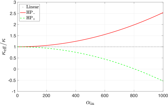
Figure 4: The total effective dissipation of the linearized models Eq. (8a) (red) and Eq. (8b) (dashed green) that correspond to the cases, where the majority of the TLSs are in the ground state/excited state, respectively. They are compared to the case of pure linear dissipation (black dots). Here we assume the system to be a simple cavity with $H_{\mathcal{S}}=\omega_{\mathrm{c}}c^{\dagger}c$. In the units of $\kappa$, the parameters are $\Delta=\omega_{\mathrm{p}}-\omega_{\mathrm{c}}=20$ and $\kappa_{N}=1.5\times 10^{-4}$.

Appendix D Fluctuation spectrum of the nonlinear model

Assuming that, in addition to the strong coherent tone, the dynamics of the system is affected by thermal fluctuations of both the bosonic and the TLS baths degrees of freedom, we evaluate here the spectrum of these fluctuations focusing on the $\mathrm{HP}_{-}$ case (an analogous derivation holds for the $\mathrm{HP}_{+}$ mapping). The fluctuation spectrum

$$S_{\omega}^{\theta}=\frac{1}{2}\Braket{\left\{X_{\omega}^{\theta},X_{-\omega}^{\theta}\right\}},$$ (30)

with $X_{\omega}^{\theta}=1/\sqrt{2}\left(a_{-\omega}^{\dagger}e^{i\theta}+a_{\omega}e^{-i\theta}\right)$, can be obtained by Fourier transforming the QLE given by Eq. (8a) and its Hermitian conjugate

$$\left[-i\left(\omega+\Delta\right)+\frac{\kappa}{2}+2\kappa_{N}\left|\alpha\right|^{2}\right]a_{\omega}+\kappa_{N}\alpha^{2}a_{-\omega}^{\dagger}=\sqrt{\kappa}a_{\mathrm{in},\omega}+2\sqrt{\kappa_{N}}\alpha^{*}a_{\mathrm{in},\omega}^{\mathrm{TLS}}$$ (31a)

$$\left[-i\left(\omega-\Delta\right)+\frac{\kappa}{2}+2\kappa_{N}\left|\alpha\right|^{2}\right]a_{-\omega}^{\dagger}+\kappa_{N}\alpha^{*2}a_{\omega}=\sqrt{\kappa}a_{\mathrm{in},-\omega}^{\dagger}+2\sqrt{\kappa_{N}}\alpha a_{\mathrm{in},-\omega}^{\mathrm{TLS}\dagger}$$ (31b)

with the usual convention for the Fourier transform, according to which $a_{t}\xmapsto{\mathrm{FT}}a_{\omega}$ and $a_{t}^{\dagger}\xmapsto{\mathrm{FT}}a^{\dagger}_{-\omega}$.

Defining

$$A =-i\left(\omega+\Delta\right)+\frac{\kappa}{2}+2\kappa_{N}\left|\alpha\right|^{2},$$ (32a)

$$B =\kappa_{N}\alpha^{2},$$ (32b)

$$C =-i\left(\omega-\Delta\right)+\frac{\kappa}{2}+2\kappa_{N}\left|\alpha\right|^{2},$$ (32c)

the QLE for the system can be expressed as

$$\begin{pmatrix}a_{\omega}\\ a_{-\omega}^{\dagger}\end{pmatrix}=\frac{1}{AC-\left|B\right|^{2}}\begin{pmatrix}C&-B\\ -B^{*}&A\end{pmatrix}\begin{pmatrix}\sqrt{\kappa}a_{\mathrm{in},\omega}+2\sqrt{\kappa_{N}}\alpha^{*}a_{\mathrm{in},\omega}^{\mathrm{TLS}}\\ \sqrt{\kappa}a_{\mathrm{in},-\omega}^{\dagger}+2\sqrt{\kappa_{N}}\alpha a_{\mathrm{in},-\omega}^{\mathrm{TLS}\dagger}\end{pmatrix}$$ (33)

and

$$a_{\omega} =\chi_{\mathrm{d}}\left(\omega\right)a_{\mathrm{in},\omega}+\chi_{\mathrm{x}}\left(\omega\right)a_{\mathrm{in},-\omega}^{\dagger}+\chi_{\mathrm{d}}^{\mathrm{TLS}}\left(\omega\right)a_{\mathrm{in},\omega}^{\mathrm{TLS}}+\chi_{\mathrm{x}}^{\mathrm{TLS}}\left(\omega\right)a_{\mathrm{in},-\omega}^{\mathrm{TLS}\dagger},$$ (34a)

$$a_{-\omega}^{\dagger} =\chi_{\mathrm{x}}^{*}\left(-\omega\right)a_{\mathrm{in},\omega}+\chi_{\mathrm{d}}^{*}\left(-\omega\right)a_{\mathrm{in},-\omega}^{\dagger}+\chi_{\mathrm{x}}^{\mathrm{TLS*}}\left(-\omega\right)a_{\mathrm{in},\omega}^{\mathrm{TLS}}+\chi_{\mathrm{d}}^{\mathrm{TLS*}}\left(-\omega\right)a_{\mathrm{in},-\omega}^{\mathrm{TLS}\dagger},$$ (34b)

where

$$\chi_{\mathrm{d}}\left(\omega\right) =\sqrt{\kappa}C(AC-\left|B\right|^{2})^{-1},$$ (35a)

$$\chi_{\mathrm{x}}\left(\omega\right) =-\sqrt{\kappa}B(AC-\left|B\right|^{2})^{-1},$$ (35b)

$$\chi_{\mathrm{d}}^{\mathrm{TLS}}\left(\omega\right) =2\sqrt{\kappa_{N}}\alpha^{*}C(AC-\left|B\right|^{2})^{-1},$$ (35c)

$$\chi_{\mathrm{x}}^{\mathrm{TLS}}\left(\omega\right) =-2\sqrt{\kappa_{N}}\alpha B(AC-\left|B\right|^{2})^{-1}.$$ (35d)

If we assume that the thermal populations of the baths are given by $\Braket{a_{\mathrm{in},\omega}a_{\mathrm{in},\omega^{\prime}}^{\dagger}}=\left(n_{\mathrm{th}}+1\right)\delta\left(\omega-\omega^{\prime}\right)$ and $\Braket{a_{\mathrm{in},\omega}^{\mathrm{TLS}}a_{\mathrm{in},\omega^{\prime}}^{\mathrm{TLS}\dagger}}=\left(n_{\mathrm{th}}^{\mathrm{TLS}}+1\right)\delta\left(\omega-\omega^{\prime}\right)$, the cavity spectrum can be written as

$$\begin{split}S_{\omega}^{\theta}=&\,\frac{1}{4}\left[\left(\left|\chi_{\mathrm{d}}\left(\omega\right)\right|^{2}+\left|\chi_{\mathrm{x}}\left(-\omega\right)\right|^{2}\right)\Braket{\left\{a_{\mathrm{in},\omega},a_{\mathrm{in},\omega}^{\dagger}\right\}}+\left(\left|\chi_{\mathrm{d}}\left(-\omega\right)\right|^{2}+\left|\chi_{\mathrm{x}}\left(\omega\right)\right|^{2}\right)\Braket{\left\{a_{\mathrm{in},-\omega}^{\dagger},a_{\mathrm{in},-\omega}\right\}}\right]\\ &+\frac{1}{4}\Big{[}\left(\chi_{\mathrm{d}}\left(\omega\right)\chi_{\mathrm{x}}\left(-\omega\right)e^{-i2\theta}+\chi_{\mathrm{d}}^{*}\left(\omega\right)\chi_{\mathrm{x}}^{*}\left(-\omega\right)e^{i2\theta}\right)\Braket{\left\{a_{\mathrm{in},\omega},a_{\mathrm{in},\omega}^{\dagger}\right\}}\\ &\qquad+\left(\chi_{\mathrm{d}}\left(-\omega\right)\chi_{\mathrm{x}}\left(\omega\right)e^{-i2\theta}+\chi_{\mathrm{d}}^{*}\left(-\omega\right)\chi_{\mathrm{x}}^{*}\left(\omega\right)e^{i2\theta}\right)\Braket{\left\{a_{\mathrm{in},-\omega}^{\dagger},a_{\mathrm{in},-\omega}\right\}}\Big{]}\\ &+\frac{1}{4}\Big{[}\left(\left|\chi_{\mathrm{d}}^{\mathrm{TLS}}\left(\omega\right)\right|^{2}+\left|\chi_{\mathrm{x}}^{\mathrm{TLS}}\left(-\omega\right)\right|^{2}\right)\Braket{\left\{a_{\mathrm{in},\omega}^{\mathrm{TLS}},a_{\mathrm{in},\omega}^{\mathrm{TLS}\dagger}\right\}}\\ &\qquad+\left(\left|\chi_{\mathrm{d}}^{\mathrm{TLS}}\left(-\omega\right)\right|^{2}+\left|\chi_{\mathrm{x}}^{\mathrm{TLS}}\left(\omega\right)\right|^{2}\right)\Braket{\left\{a_{\mathrm{in},-\omega}^{\mathrm{TLS}\dagger},a_{\mathrm{in},-\omega}^{\mathrm{TLS}}\right\}}\Big{]}\\ &+\frac{1}{4}\Big{[}\left(\chi_{\mathrm{d}}^{\mathrm{TLS}}\left(\omega\right)\chi_{\mathrm{x}}^{\mathrm{TLS}}\left(-\omega\right)e^{-i2\theta}+\chi_{\mathrm{d}}^{\mathrm{TLS}*}\left(\omega\right)\chi_{\mathrm{x}}^{\mathrm{TLS}*}\left(-\omega\right)e^{i2\theta}\right)\Braket{\left\{a_{\mathrm{in},\omega}^{\mathrm{TLS}},a_{\mathrm{in},\omega}^{\mathrm{TLS}\dagger}\right\}}\\ &\qquad+\left(\chi_{\mathrm{d}}^{\mathrm{TLS}}\left(-\omega\right)\chi_{\mathrm{x}}^{\mathrm{TLS}}\left(\omega\right)e^{-i2\theta}+\chi_{\mathrm{d}}^{\mathrm{TLS}*}\left(-\omega\right)\chi_{\mathrm{x}}^{\mathrm{TLS}*}\left(\omega\right)e^{i2\theta}\right)\Braket{\left\{a_{\mathrm{in},-\omega}^{\mathrm{TLS}\dagger},a_{\mathrm{in},-\omega}^{\mathrm{TLS}}\right\}}\Big{]}\\ =&\,\frac{1}{2}\Big{[}\left|\chi_{\mathrm{d}}\left(\omega\right)\right|^{2}+\left|\chi_{\mathrm{d}}\left(-\omega\right)\right|^{2}+\left|\chi_{\mathrm{x}}\left(\omega\right)\right|^{2}+\left|\chi_{\mathrm{x}}\left(-\omega\right)\right|^{2}\\ &\qquad+2\cos\left(\theta+\phi\right)\left|\chi_{\mathrm{d}}\left(\omega\right)\chi_{\mathrm{x}}\left(-\omega\right)+\chi_{\mathrm{d}}\left(-\omega\right)\chi_{\mathrm{x}}\left(\omega\right)\right|\Big{]}\left(n_{\mathrm{th}}+\frac{1}{2}\right)\\ &+\frac{1}{2}\Big{[}\left|\chi_{\mathrm{d}}^{\mathrm{TLS}}\left(\omega\right)\right|^{2}+\left|\chi_{\mathrm{d}}^{\mathrm{TLS}}\left(-\omega\right)\right|^{2}+\left|\chi_{\mathrm{x}}^{\mathrm{TLS}}\left(\omega\right)\right|^{2}+\left|\chi_{\mathrm{x}}^{\mathrm{TLS}}\left(-\omega\right)\right|^{2}\\ &\qquad+2\cos\left(\theta+\phi^{\mathrm{TLS}}\right)\left|\chi_{\mathrm{d}}^{\mathrm{TLS}}\left(\omega\right)\chi_{\mathrm{x}}^{\mathrm{TLS}}\left(-\omega\right)+\chi_{\mathrm{d}}^{\mathrm{TLS}}\left(-\omega\right)\chi_{\mathrm{x}}^{\mathrm{TLS}}\left(\omega\right)\right|\Big{]}\left(n_{\mathrm{th}}^{\mathrm{TLS}}+\frac{1}{2}\right),\\ \end{split}$$ (36)

where $\phi^{(\mathrm{TLS})}=\mathrm{Arg}\left[\chi_{\mathrm{d}}^{(\mathrm{TLS})}\left(\omega\right)\chi_{\mathrm{x}}^{(\mathrm{TLS})}\left(-\omega\right)+\chi_{\mathrm{d}}^{(\mathrm{TLS})}\left(-\omega\right)\chi_{\mathrm{x}}^{(\mathrm{TLS})}\left(\omega\right)\right]$. In Fig. 5(a) we have plotted the cavity spectrum for the HP_-, and the spectrum related to HP₊ coupling derived from Eq. (8b) is presented in Fig. 5(b).

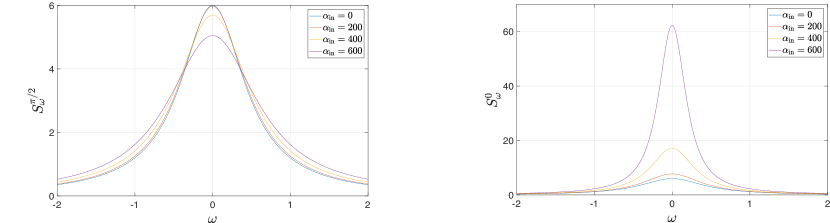
Figure 5: The cavity spectra related to the Holstein-Primakoff couplings (a) HP_- and (b) HP₊ for the largest uncertainty quadrature ($\theta=\pi/2$ and $\theta=0$, respectively). In (a) the linewidth widens as $\alpha_{\mathrm{in}}$ becomes larger, whereas in (b) the linewidth becomes narrower. Here the thermal populations of the bosonic and TLS baths are $n_{\mathrm{th}}=n_{\mathrm{th}}^{\mathrm{TLS}}=1$, and in the units of $\kappa$, the other parameters are $\Delta=20$ and $\kappa_{N}=1.5\times 10^{-4}$.

References

• Leggett (2005) A. J. Leggett, Science 307, 871 (2005).
• Zurek (1991) W. H. Zurek, Phys Today 44, 36 (1991).
• Leggett et al. (1987) A. J. Leggett, et al., Rev. Mod. Phys. 59, 1 (1987).
• Breuer and Petruccione (2007) H.-P. Breuer and F. Petruccione, The Theory of Open Quantum Systems (OUP Oxford, 2007).
• Breuer et al. (2016) H.-P. Breuer, et al., Rev. Mod. Phys. 88, 1021 (2016).
• Ishizaki et al. (2010) A. Ishizaki, et al., Phys. Chem. Chem. Phys. 12, 7319 (2010).
• Leskinen et al. (2010) M. J. Leskinen, et al., New J Phys 12 (2010).
• Massel et al. (2013) F. Massel, et al., New J Phys 15, 045018 (2013).
• Visuri et al. (2014) A. M. Visuri, et al., PRA 90, 051603 (2014).
• Ano (2012) The Nobel Prize in Physics 2012 (2012), URL https://www.nobelprize.org/nobel_prizes/physics/laureates/2012/press.html.
• Wiseman and Milburn (2010) H. M. Wiseman and G. J. Milburn, Quantum Measurement and Control (Cambridge University Press, 2010).
• Nielsen and Chuang (2010) M. A. Nielsen and I. L. Chuang, Quantum Computation and Quantum Information, 10th Anniversary Edition (Cambridge University Press, 2010).
• Clerk et al. (2010) A. A. Clerk, et al., Rev. Mod. Phys. 82, 1155 (2010).
• Abbott et al. (2016) B. P. Abbott, et al., Phys. Rev. Lett. 116, 061102 (2016).
• Wallraff et al. (2004) A. Wallraff, et al., Nature 431, 162 (2004).
• Sillanpää et al. (2007) M. A. Sillanpää, J. I. Park, and R. W. Simmonds, Nature 449, 438 (2007).
• Majer et al. (2007) J. Majer, et al., Nature 449, 443 (2007).
• Schoelkopf and Girvin (2008) R. J. Schoelkopf and S. M. Girvin, Nature 451, 664 (2008).
• Poyatos et al. (1996) J. F. Poyatos, J. I. Cirac, and P. Zoller, Phys. Rev. Lett. 77, 4728 (1996).
• Teufel et al. (2011) J. D. Teufel, et al., Nature 475, 359 (2011).
• Wollman et al. (2015) E. E. Wollman, et al., Science 349, 952 (2015).
• Pirkkalainen et al. (2015) J. M. Pirkkalainen, et al., Phys. Rev. Lett. 115, 243601 (2015).
• Lecocq et al. (2015) F. Lecocq, et al., Phys. Rev. X 5, 041037 (2015).
• Massel et al. (2011) F. Massel, et al., Nature 480, 351 (2011).
• Ockeloen-Korppi et al. (2016) C. F. Ockeloen-Korppi, et al., Phys. Rev. X 6, 041024 (2016).
• Metelmann and Clerk (2015) A. Metelmann and A. A. Clerk, Phys. Rev. X 5, 021025 (2015).
• Mirrahimi et al. (2014) M. Mirrahimi, et al., New J Phys 16, 045014 (2014).
• Leghtas et al. (2015) Z. Leghtas, et al., Science 347, 853 (2015).
• Zolfagharkhani et al. (2005) G. Zolfagharkhani, et al., Phys. Rev. B 72, 224101 (2005).
• Arcizet et al. (2009) O. Arcizet, et al., Phys. Rev. A 80, 021803 (2009).
• Eichler et al. (2011) A. Eichler, et al., Nature Nanotech 6, 339 (2011).
• Suh et al. (2012) J. Suh, et al., Nano Lett. 12, 6260 (2012).
• Singh et al. (2016) V. Singh, et al., Phys. Rev. B 93, 245407 (2016).
• Simmonds et al. (2004) R. W. Simmonds, et al., Phys. Rev. Lett. 93, 077003 (2004).
• Martinis et al. (2005) J. M. Martinis, et al., Phys. Rev. Lett. 95, 210503 (2005).
• Ashhab et al. (2006) S. Ashhab, J. R. Johansson, and F. Nori, New J Phys 8, 103 (2006).
• O’Connell et al. (2008) A. D. O’Connell, et al., Appl. Phys. Lett. 92, 112903 (2008).
• Gao et al. (2008) J. Gao, et al., Appl. Phys. Lett. 92, 212504 (2008).
• Neill et al. (2013) C. Neill, et al., Appl. Phys. Lett. 103, 072601 (2013).
• Phillips (1987) W. A. Phillips, Reports on Progress in Physics 50, 1657 (1987).
• Quintana et al. (2014) C. M. Quintana, et al., Appl. Phys. Lett. 105, 062601 (2014).
• Kleiman et al. (1987) R. N. Kleiman, G. Agnolet, and D. J. Bishop, Phys. Rev. Lett. 59, 2079 (1987).
• Lindkvist and Johansson (2014) J. Lindkvist and G. Johansson, New J Phys 16, 055018 (2014).
• Fischer et al. (2017) K. A. Fischer, et al., Nat. Phys. 13, 649 (2017).
• Grabovskij et al. (2012) G. J. Grabovskij, et al., Science 338, 232 (2012).
• Holder et al. (2013) A. M. Holder, et al., Phys. Rev. Lett. 111, 065901 (2013).
• Stefanucci and van Leeuwen (2014) G. Stefanucci and R. van Leeuwen, Nonequilibrium Many-Body Theory of Quantum Systems (Cambridge University Press, 2014).