Competition and Complexity in Amphiphilic Polymer Morphology

Abstract

The strong Functionalized Cahn Hilliard equation models self assembly of amphiphilic polymers in solvent. It supports codimension one and two structures that each admit two classes of bifurcations: pearling, a short-wavelength in-plane modulation of interfacial width, and meandering, a long-wavelength instability that induces a transition to curve-lengthening flow. These two potential instabilities afford distinctive routes to changes in codimension and creation of non-codimensional defects such as end caps and $Y$-junctions. Prior work has characterized the onset of pearling, showing that it couples strongly to the spatially constant, temporally dynamic, bulk value of the chemical potential. We present a multiscale analysis of the competitive evolution of codimension one and two structures of amphiphilic polymers within the $H^{-1}$ gradient flow of the strong Functionalized Cahn Hilliard equation. Specifically we show that structures of each codimension transition from a curve lengthening to a curve shortening flow as the chemical potential falls through a corresponding critical value. The differences in these critical values quantify the competition between the morphologies of differing codimension for the amphiphilic polymer mass. We present a bifurcation diagram for the morphological competition and compare our results quantitatively to simulations of the full system and qualitatively to simulations of self-consistent mean field models and laboratory experiments. In particular we propose that the experimentally observed onset of morphological complexity arises from a transient passage through pearling instability while the associated flow is in the curve lengthening regime.

toltxlabel *[BilayerPearl-]../../BilayerPearling/PearlingBilayerV35/PearlingforBilayerV35

1 Introduction

Amphiphilic molecules are increasingly important in synthetic chemistry where they permit molecular level control of the self assembly of materials with desirable ionic and electronic conduction properties, [4]. A molecule is amphiphilic with respect to a solvent if it is comprised of two components, one of which has an energetically favorable or hydrophilic interaction with the solvent and the other with an energetically unfavorable or hydrophobic interaction. There is a growing literature for the construction and characterization of amphiphilic diblock polymers comprised of polymer chains formed from adjustable lengths of hydrophilic and hydrophobic polymers covalently bonded together. Amphiphilic molecules are typically characterized by the Flory-Huggins parameters indicating the strength of the hydrophobic/hydrophilic interactions and by the aspect ratio of the two components, [13].

When immersed in solvent, amphiphilic polymers self assemble into a wide variety of structures with diverse morphologies that include codimension one bilayers (hollow vesicles), codimension two filaments (solid rods or cylinders), codimension three micelles (solid spheres), and various defect structures with no well defined codimension such as end-caps, “Y” junctions, and mixed morphologies. The bifurcation structure of these mixtures has been experimentally investigated for a variety of different diblock structures. Two seminal experiments, presented in Figure 1, have partially unfolded this bifurcation structure by studying the impact of varying the solvent blend to modify strength of the amphiphilic interaction, [10], and of varying the aspect ratio of amphiphilic polymer, [16]. Increasing the strength of the amphiphilic interaction and decreasing the aspect ratio of the minority phase produce similar results: a sequence of bifurcations in which codimension-one bilayers yield to codimension-two filaments which yield in turn to codimension-three micelles. In some experiments these codimensional structures are reported to coexist for a range of parameter values while others show regions of “morphological complexity” characterized by an abundance of defects.

In this paper we analyze the coexistence, bifurcation, and longtime evolution of well-separated, defect free, codimension one and two structures within the context of the $H^{-1}$ gradient flows of the strong scaling of the Functionalized Cahn Hilliard free energy. We use multiscale analysis to derive the curvature driven evolution of codimension one and codimension two structures that are sufficiently far from self intersection. We show that the evolution of morphologies of distinct codimension couples through their exchange of amphiphilic molecules with the bulk. The bulk chemical potential is spatially constant and varies temporally on a slow time scale. Most significantly, codimension one and two structures switch between a regularized curve lengthening and a curve shortening evolution as the bulk chemical potential passes through critical values. This dichotomy presents a mechanism for morphological competition in which structures of one codimension grow at the expense of the other. This suggests that, in the absence of defects, the coexistence of structures with distinct codimensions is not generic however the resolution into structures of homogeneous codimension may require a substantial transient. This finding is supported by experimental results, see [17], which report that transient structures can persist for months.

There are two mechanisms for a codimension one or two structure to develop an initial defect: self intersection and pearling. Pearling bifurcations are high-frequency tangential modulations of the width of the codimensional structure. In a companion paper, [18], we characterized the onset of the pearling bifurcation, showing that within the strong scaling of the functionalized Cahn Hilliard free energy the onset of pearling is independent of the shape of the codimension one or two structure, but couples to the transient value of the bulk chemical potential. Self intersections can be non-local, arising when the initial intersection points are well separated in distance measured along the curve, as in a figure-8 intersection. They can also be local, as arises when a surface develops large curvatures, such as when the radius of a sphere tends to zero. In both cases the self intersections arise from the evolution of the underlying manifold that characterizes the structure. Curve-shortening flows render the manifold smaller and drive their curvatures towards constant values. Conversely, curve lengthening flows act like backward heat equations for the interfacial curvature and are well known to be locally ill-posed. We derive a regularized curve lengthening flow that includes a higher-order surface diffusion. The regularized curve lengthening is locally well posed evolution, but causes the underlying curve to grow and “meander” or buckle, and typically leads to finite-time non-local self intersections. In both cases the finite-time singularities can be arrested by the quenching element of the flow which slows the normal velocity as the far-field chemical potential approaches an equilibrium value. Depending upon initial conditions, our results can predict either a relaxation to an equilibrium state or provide the mechanisms for the generation of defect states.

Our analysis is particularly relevant to the study of morphologies derived from casting processes in which an initial suspension of amphiphilic molecules, reflecting a high bulk chemical potential, nucleates out structures of various codimension which initially grow, absorbing the amphiphilic molecules from the bulk suspension and lowering the bulk chemical potential. As the chemical potential falls it may trigger or inhibit pearling bifurcations in one or both codimensions, or trigger transitions from the regularized curve lengthening to curve shortening. We compare our asymptotic results to simulations of the full system, to simulations of self-consistent mean-field density functional models of amphiphilic polymer melts, and to experimental bifurcation diagrams.

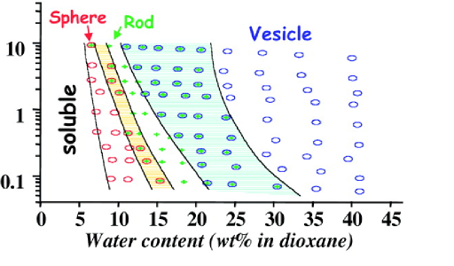
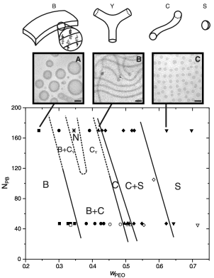
Figure 1: Morphological bifurcation diagrams for two classes of amphiphilic polymers in solvent. (left) Morphology of Polystyrene (PS) - Polyacrylic acid (PAA) diblocks as function of increasing water content in water-dioxane solvent blend (horizontal axis) and polymer %-weight fraction of the overall mixture (vertical axis). Increased water volume fraction drives bifurcation to lower codimensional morphologies without inducing pearling. From [10]. Reprinted with permission from AAAS. (right) Morphology of amphiphilic Polyethylene oxide (PEO) - Polybutadiene (PB) diblock suspension as function of the PEO weight fraction, $w_{\rm PEO}$ (horizontal axis) for molecular weights of PB fixed at $N_{\rm PB}=45$ and $170$ (vertical axis). Defect loaded phases are observed for the higher value of $N_{\rm PB}$. Images of polymer morphologies are included inset, as well as schematic representations of codimension one, two, and three morphologies and ‘Y’ junctions. From [16]. Reprinted with permission from AAAS.

1.1 The Functionalized Cahn Hilliard free energy

The Functionalized Cahn Hilliard (FCH) free energy models the free energy of a binary mixture of an amphiphilic molecule and a solvent. It supports stable network morphologies including codimension one bilayers and codimension two filaments as well as pearled morphologies and the defects such as end-caps and $Y$-junctions, [21, 14, 7, 11, 22]. The FCH free energy takes the form

$${\cal F}(u):=\int\limits_{\Omega}\frac{1}{2}\left(\varepsilon^{2}\Delta u-W^{\prime}(u)\right)^{2}-\varepsilon^{p}\left(\frac{\varepsilon^{2}\eta_{1}}{2}|\nabla u|^{2}+\eta_{2}W(u)\right)\,dx,$$ (1.1)

where $W$ is a smooth double-well potential with local minima at $u=b_{\pm}$ with $b_{-}<b_{+}$. The two wells have unequal depths that are normalized so that $W(b_{-})=0>W(b_{+})$ and the left well is non-degenerate in the sense that $\alpha_{-}:=W^{\prime\prime}(b_{-})>0$. The value of $\alpha_{-}$ is a key parameter that controls the rate of exchange of amphiphilic molecules between the bulk and the various morphologies. Here $\varepsilon\ll 1$ is small parameter corresponding to the ratio of length of the amphiphilic molecule to the domain size, $u=b_{-}$ is associated to a bulk solvent phase, while the quantity $u-b_{-}>0$ is proportional to the density of the amphiphilic phase. The first term in the integrand of (1.1) is called the Willmore or the quadratic term, as it denotes the square of a variational derivative of a Cahn Hilliard type free energy. The quadratic term is positive, and we refer to the class of $u\in H^{2}(\Omega)$ for which the residual of the quadratic term is small compared to $\varepsilon$ as morphologies. The second grouping of terms in the integrand, multiplied by $\varepsilon^{p}$, are called the functionalization terms. The strong and weak scalings of the FCH free energy correspond to the choice $p=1$ and $p=2$, respectively in (1.1) and represent two natural choices of distinguished limits between the residual of the quadratic term and the typical scaling of the functionalization terms. In the strong scaling of the FCH, the $O(\varepsilon)$ functionalization terms typically dominate the generically $O(\varepsilon^{2})$ residuals from the quadratic terms, in the weak scaling both terms balance at $O(\varepsilon^{2})$. The analysis of this paper focuses on the strong scaling of the FCH free energy for which the bifurcation analysis is more accessible.

The functionalization parameters $\eta_{1}$ and $\eta_{2}$ characterize key properties of the amphiphilic molecules. Specifically $\eta_{1}>0$ models the strength of the hydrophilic interaction, modeling the propensity of amphiphilic molecules to form monolayers by rewarding increases in interfacial area or curve length with a decrease in free energy. The parameter $\eta_{2}\in\mathbb{R}$ encodes the aspect ratio of the amphiphilic molecule, as discussed in section 4.3. Equivalently these parameters are analogous to the surface and volume energies typical of models of charged solutes in confined domains, see [24] and particularly equation (67) of [3]. With these parameter choices the minus sign in front of the functionalization terms has great significance – it incorporates the propensity of the amphiphilic surfactant phase to drive the creation of interface. Indeed, experimental tuning of solvent quality identifies molecular level phase separation and self assembly in amphiphilic mixtures with the onset of negative values of surface tension in mesoscale agglomerates, [25] and [26].

Prior work on FCH gradient flows has focused on the weak scaling, corresponding to $p=2$ in (1.1). In [7] the authors derived the geometric evolution of bilayers at the quenched mean-curvature flow on the $O(\varepsilon^{-1})$ time scale and as a surface area preserving Willmore flow on the $O(\varepsilon^{-2})$ time scale. The geometric evolution of codimension two structures was derived in [8], obtaining a curvature driven competitive geometric evolution of the filament curve on the $O(\varepsilon^{-1})$ time scale and a length-preserving Willmore type flow on the $O(\varepsilon^{-2})$ time scale. Moreover, it was found that the codimension one and two structures can co-exist on the faster $O(\varepsilon^{-1})$ time scale in the weak FCH, but compete on the longer $O(\varepsilon^{-2})$ time scale. However, rigorous investigation of the pearling bifurcation in the weak FCH is complicated by its leading order coupling to the curvature of the underlying curves. Conversely in the strong scaling of the FCH, the pearling bifurcation is independent of morphology and was rigorously characterized in [18] for a wide class of codimension one and two structures.

In the remainder of this paper we consider the strong scaling of the FCH free energy. Fixing $\Omega=[0,L]^{d}\subset{\mathbb{R}}^{d}$ for $d=2,3,\ldots$ and applying periodic boundary conditions to $H^{4}(\Omega)$, the first variation of ${\cal F}$, also called the chemical potential $\mu,$ associated to a spatial distribution $u\in H^{4}(\Omega)$ takes the form

$$\mu:=\frac{\delta{\cal F}}{\delta u}(u) =(\varepsilon^{2}\Delta-W^{\prime\prime}(u)+\varepsilon\eta_{1})(\varepsilon^{2}\Delta u-W^{\prime}(u))+\varepsilon\eta_{d}W^{\prime}(u),$$ (1.2)

where $\eta_{d}:=\eta_{1}-\eta_{2}$. The Functionalized Cahn Hilliard equation is the associated $H^{-1}$ gradient flow,

$$u_{t}=\Delta\mu(u),$$ (1.3)

supplemented with periodic boundary conditions on $\Omega$. The choice of the $H^{-1}$ gradient is a reflection of its status as the simplest local gradient that preserves mass. The mathematical focus of the paper is on the multiscale analysis of the evolution codimension one and two structures. On the $O(\varepsilon^{-1})$ time scale we find that the $H^{-1}$ gradient flow drives well separated filament and bilayer structures through a competitive, mean-curvature driven flow mediated through the common value of the spatially constant far-field chemical potential, $\mu_{1}$ defined in (2.17). We show in section 2 that the nonlocal Mullins-Sekerka problem familiar to Cahn Hilliard evolution is present but is unforced, and on the long time scales we consider the far-field chemical potential relaxes to a trivial, spatially-constant for both codimension one bilayer and codimension two filament morphologies. As a consequence, the geometric evolution is local.

While spatially constant, the far-field chemical potential $\mu_{1}=\mu_{1}(t)$, is temporally dynamic and is linearly proportional to the density of free amphiphilic molecules in the bulk. It serves as a key bifurcation parameter, triggering two potential types of instability for each codimension of morphology. Indeed, in [15] it is shown for the FCH free energy that the pearling and self intersection via geometric motion are the only possible mechanisms to generate defects in bilayers. In the companion paper, [18], a sharp condition for pearling stability is derived that relates the chemical potential to the parameter $\eta_{d}$ and constants that depend implicitly on the form of the double-well $W$. Specifically the bilayers are stable with respect to the pearling bifurcation if and only if

$$\mu_{1}S_{b}+\eta_{d}\lambda_{b,0}\left\lVert\psi_{b,0}\right\rVert_{2}^{2}<0,$$ (1.4)

and similarly filaments are pearling stable if and only if

$$\mu_{1}S_{{\it f}}+\eta_{d}\left(\left\lVert\psi_{{{\it f}},0,0}^{\prime}\right\rVert_{L_{R}}^{2}+\lambda_{{{\it f}},0,0}\left\lVert\psi_{{{\it f}},0,0}\right\rVert_{L_{R}}^{2}\right)<0,$$ (1.5)

where $\lambda_{b,0}$ is the ground-state eigenvalue of the linear operator $L_{b,0}$ , defined in (2.7), with eigenfunction $\psi_{b,0}$, and $\lambda_{{{\it f}},0,0}$ is the ground state eigenvalue of the linear operator $L_{{{\it f}},0,0}$, defined in (3.16), with the corresponding eigenfunction $\psi_{{{\it f}},0,0}$. The constants $S_{b},S_{{\it f}}$ are the shape factors of the bilayers and the filaments, respectively, defined by the relations

$$S_{b}:=\int_{\mathbb{R}}\Phi_{b,1}W^{\prime\prime\prime}(\phi_{b})\psi_{b,0}^{2}\,dz,\quad S_{{\it f}}:=2\pi\int_{0}^{\infty}\Phi_{{{\it f}},1}W^{\prime\prime\prime}(\phi_{{\it f}})\psi_{{{\it f}},0,0}^{2}\,RdR.$$ (1.6)

Here $\phi_{b}$ and $\phi_{{\it f}}$ are the bilayer and filament profiles, defined in (2.6) and (3.10), while $\Phi_{b,1}$ and $\Phi_{{{\it f}},1}$, defined in (2.8) and (3.17), encode the impact of a change in chemical potential on the shape of the bilayer and filament, respectively. For each codimension, if the shape factor is negative then pearling stability is favored by large (positive) values of $\mu_{1}$, while if it is positive then pearling stability is favored for small (negative) values of $\mu_{1}$. In [22] the existence of pearled codimension one circular and flat equilibrium was demonstrated in $\mathbb{R}^{2}$ for the strong FCH.

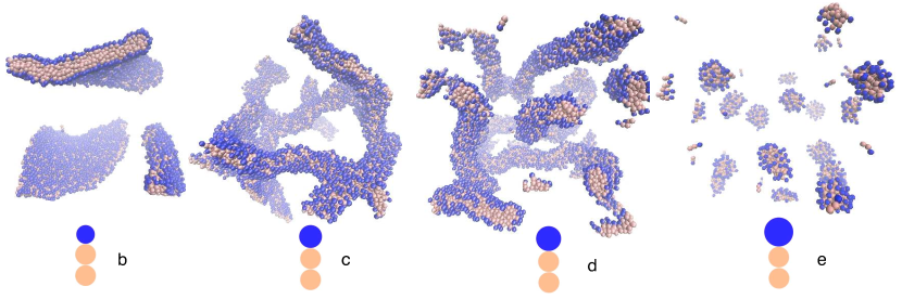
Figure 2: Molecular dynamics simulations of amphiphilic molecules with distinct aspect ratios. Increasing the size of the hydrophilic head group, relative to a fixed tail leads to a preference for morphologies with increasing codimensions: (b) bilayers with edge caps (codim 1), (c) branched filaments (codim 2), (d) unbranched filaments (codim 2), and (e) micelles (codim 3). Morphologies with higher codimension have a higher density of free-floating amphiphilic molecules in the far-field (bulk), corresponding to a higher critical value of $\mu_{1}$. Reprinted from [6], with permission from Elsevier.

1.2 Summary of Analytical Results

Our main analytical result is the derivation of curvature driven flow laws valid on slow time $\tau=\varepsilon t$ for codimension one and two structures embedded in $\Omega\subset\mathbb{R}^{3}$ via a multiscale analysis. Bilayer and filament morphologies are defined as dressings of collections of admissible interfaces and curves, respectively. We consider an admissible codimension one interface $\Gamma_{b}$, see Definition 2.1, with $O(1)$ area and codimension two curve $\Gamma_{{\it f}}$, see Definition 3.1, with $O(\varepsilon^{-1})$ length. We assume the reaches of these two classes of surfaces, as defined in (2.2) and (3.4) respectively, are all disjoint and introduce the composite solution defined in (4.2). The evolution of these composite solutions under the gradient flow (1.3) is parameterized at leading order by the triple $(\Gamma_{b},\Gamma_{{\it f}},\mu_{1})$ according to their $\varepsilon$-scaled normal velocities

$$V_{b} =\nu_{b}(\mu_{1}-\mu_{b}^{*})H_{0}+\varepsilon k_{b}\Delta_{s}H_{0},$$ (1.7)

$${\bf V}_{{\it f}} =-\left[\nu_{{\it f}}(\mu_{1}-\mu_{{\it f}}^{*})\vec{\kappa}+\varepsilon k_{f}\partial_{s}^{2}\vec{\kappa}\right].$$ (1.8)

Here we have introduced the mean curvature $H_{0}$ and Laplace-Beltrami operator $\Delta_{s}$ of $\Gamma_{b}$ and vector curvature $\vec{\kappa}=(\kappa_{1},\kappa_{2})$ and surface diffusion $\partial_{s}^{2}$ of $\Gamma_{{\it f}}$. On this slow time $\tau=\varepsilon t$, the chemical potential satisfies

$$\frac{d\mu_{1}}{d\tau}=-\frac{\alpha_{-}^{2}}{|\Omega|}\Bigg{[} m_{b}\int_{\Gamma_{b}}\nu_{b}\left({\mu_{1}}-\mu_{b}^{*}\right)H_{0}^{2}-\varepsilon k_{b}|\nabla_{s}H_{0}|^{2}\,ds$$ (1.9)

$$+2\pi m_{{\it f}}\varepsilon\int_{\Gamma_{{\it f}}}\nu_{{\it f}}\left({\mu_{1}}-\mu_{{\it f}}^{*}\right)|\vec{\kappa}|^{2}-\varepsilon|\partial_{s}\vec{\kappa}_{{\it f}}|^{2}\,ds\Bigg{]}+O(\varepsilon^{2}),$$

where the constants $\nu_{b}>0$, $k_{b}>0$, and $m_{b}>0$, are defined in (2.51) while $\nu_{{\it f}}>0$, $k_{{\it f}}>0$, and $m_{{\it f}}>0$ defined in (3.77). While the surface diffusion terms are formally lower order, they are leading order singular perturbations that keep the resulting flow locally well-posed.

The system (1.7)-(1.9) describes the competitive dynamics between codimension one and two morphologies. The key critical values

$$\mu_{b}^{*} =-\frac{k_{b}}{2\nu_{b}}(\eta_{1}+\eta_{2}),$$ (1.10)

$$\mu_{{\it f}}^{*} =\frac{k_{{\it f}}}{\nu_{f}}\eta_{1},$$ (1.11)

indicate the value of $\mu_{1}$ at which the rates of amphiphilic molecule insertion and ejection are balanced for bilayers and filaments, respectively. Specifically, if the far-field chemical potential lies above this number, then structures of the corresponding codimension will grow. Indeed, the rate of change of the area of bilayers is given by

$$\partial_{\tau}|\Gamma_{b}|=\int_{\Gamma_{b}}V_{b}H_{0}\,ds=\int_{\Gamma_{b}}\nu_{b}(\mu_{1}-\mu_{b}^{*})H_{0}^{2}-\varepsilon k_{b}|\nabla_{s}H_{0}|^{2}\,ds,$$ (1.12)

with the corresponding expression

$$\partial_{\tau}|\Gamma_{{\it f}}|=\int_{\Gamma_{{\it f}}}{\bf V}_{{\it f}}\cdot\vec{\kappa}\,ds=\int_{\Gamma_{{\it f}}}\nu_{b}(\mu_{1}-\mu_{{\it f}}^{*})|\vec{\kappa}|^{2}-\varepsilon k_{{\it f}}|\partial_{s}\vec{\kappa}|^{2}\,ds,$$ (1.13)

for the length of the filaments. The competitive dynamics system provides the leading order evolution so long as the interfaces remain admissible with disjoint reaches and the $\mu_{1}$-dependent pearling conditions (1.4)-(1.5) hold. The surface diffusion terms in (1.7)-(1.8) are relevant to mass balance only if the gradients of the curvatures become asymptotically large or if $\mu_{1}$ becomes asymptotically close to one of the critical values $\mu_{b}^{*}$ or $\mu_{{\it f}}^{*}$. In particular, it follows from (1.9) that net growth of bilayers and filaments corresponds to a decrease in $\mu_{1}$, while large curvature gradients enhance the ejection rates and increase the value of $\mu_{1}$.

Remark: For the codimension two filament term to contribute to the evolution of the chemical potential, $\mu_{1}$, at leading order, we assume that their collective length $|\Gamma_{{\it f}}|$ is $O(\varepsilon^{-1})$. Our generic assumption on the codimension one phase is the surface area $|\Gamma_{b}|=O(1)$, so that both bilayers and filaments occupy an $O(\varepsilon)$ volume fraction. This limits the applicability of the asymptotic results as the assumption of disjoint reaches becomes non-generic, and represents a significant caveat in the application of our analytical results. Since the geometric flow reduction does not apply to morphologies with defects, both a large number of short filaments or a small number of long filaments complicate the non-self intersection assumption. Our analysis applies to each disjoint component of filament morphology separately, and while $\varepsilon\ll 1$ is small, it is viewed as fixed within the model and need not be vanishingly small. A more detailed analysis of mass scaling in the $\varepsilon\to 0$ convergence issues for FCH models can be found in [9].

For $\mu_{1}>\mu_{b}^{*}$ we call the normal velocity (1.7) a regularized (codimension one) curve lengthening flow and a (codimension one) curve shortening flow if $\mu_{1}<\mu_{b}^{*}$, with similar terminology for the codimension two flow based upon the sign of $\mu_{1}-\mu_{{\it f}}^{*}.$ When the structures have a homogeneous codimension, then in the absence of singularities in the curvature flow, equation (1.9) drives the chemical potential $\mu_{1}$ to the corresponding critical value, $\mu_{b}^{*}$ or $\mu_{{\it f}}^{*}$, and the leading-order term in the geometric flow goes to zero, and the system is said to be “quenched”. To illustrate the nature of the geometric flow, it is instructive to rewrite it as a corresponding evolution equation for the curvatures. For codimension one structures in two space dimensions, up to tangential reparameterization it takes the simple form

$$\partial_{\tau}H_{0}=-(\Delta_{s}+H_{0}^{2})V_{b}=-(\Delta_{s}+H_{0}^{2})\left(\nu_{b}(\mu_{1}-\mu_{b}^{*})H_{0}+\varepsilon k_{b}\Delta_{s}H_{0}\right).$$ (1.14)

For the curve lengthening regime, the dominant term is a backward heat equation, with a fourth-order regularization and a $H_{0}^{3}$ nonlinearity with a negative (stable) coefficient. For the curve shortening regime, both differential terms are stabilizing, but the cubic nonlinearity has a positive coefficient that supports finite time singularity which may be arrested by the fourth order regularization.

In numerical simulations the curve lengthening flows, with $\mu_{1}>\mu^{*}_{b,{{\it f}}}$ show distinct regimes. For positive but $O(\varepsilon)$ values of $\mu_{1}-\mu^{*}_{b}$ the bilayer interfaces will bend and buckle at $O(1)$ length scales, leading to shapes reminiscent of a meandering river. This regime is called a “meandering flow”, and is studied rigorously in [5]. For $O(1)$ positive values of $\mu_{1}-\mu_{b}^{*}$ the curve lengthening flows can lead to growth of high-curvature regions which self intersect on a $\tau=O(1)$ length scale. For filaments this can lead to the formation of many closed loops, see Figures 2 and 3 of [16] for experimental examples or Figure 5 of this article for an example of meandering motion within the FCH gradient flow.

1.3 Competition and Morphological Complexity

Our main scientific results are the conjectured mechanisms for the morphological bifurcations observed in the casting of amphiphilic suspensions. In particular we propose a mechanism for the onset of the so-called “morphological complexity” observed in the experimental casting processes presented in Figure 1 (right). In a casting process amphiphilic molecules are dispersed (mixed) in a solvent and the mixture is allowed to relax, generically leading to self-assembly of structures with distinct codimension. For the shorter chains, $N_{PB}=45$ corresponding to the lower horizontal row of symbols, casts from molecules with increasing weight fraction of the amphiphilic PEO component ($w_{\rm PEO}$ – horizontal axis) lead to a series of codimensional bifurcations in which the self-assembly prefers structures with increasing codimension. Indeed experiments produce first bilayers (codimension one) marked (B), then bilayers coexisting with cylinders (codimension two) marked (B+C), then cylinders, then cylinders coexisting with spheres (codimension three) marked (S), and finally spheres. A similar series of codimensional bifurcations are presented in Figure 1(left) and Figure 2. In the former the bifurcations are induced by lowering the percentage of water in the water-dioxane solvent which forms the basis for the casting. In the latter they are realized within coarse-grained molecular dynamics simulations of casting processes by increasing the size of the hydrophilic head group, and hence the aspect ratio, of a simple three-group amphiphilic molecule.

We conjecture that the competitive dynamics implicit in the system (1.7)-(1.9) forms the basis for these codimensional bifurcations. In a casting process there is initially a relatively large density of dispersed amphiphilic molecules, corresponding to a high value of the far-field chemical potential $\mu_{1}$. As various structures self-organize, amphiphilic molecules are removed from the far-field and the scalar value of $\mu_{1}$ falls. The critical values $\mu_{b}^{*}$ and $\mu_{{\it f}}^{*}$, given in (1.10)-(1.11), guage the relative ability of the corresponding bilayer and filament morphologies to absorb and retain amphiphilic molecules from the far-field (bulk) environment. The morphology with the lowest corresponding critical value will, in the absence of defects, lower the value of $\mu_{1}$ and drain the mass of the morphologies with higher critical values of $\mu_{1}$. Increasing values of either $\eta_{1}$ or $\eta_{2}$ will drive $\mu_{b}$ greater than $\mu_{{\it f}}$ and trigger a competitive imbalance that favors codimension two filaments over codimension one bilayers. We argue in Section 4 that increasing the aspect ratio of the amphiphilic molecule corresponds to an increase in the value of $\eta_{2}$, while decreasing the percentage of water within the water-dioxane solvent blend corresponds to an increase in the value of $\eta_{1}$. These produce shifts in $\mu_{b,{{\it f}}}^{*}$ in agreement with bifurcation from codimension one to codimension two. The coexistence of codimension one and two structures for large parameter ranges are not supported by the analysis. However the time scale to reach equilibrium can be quite long, [17] suggest times on the order of months, and we propose that longer experimental trials may decrease the size of the regions of coexistence. We do not present an analysis of codimension three micelles within this work as they do not have a spatially extended direction that can accommodate incremental growth, rather simulations suggest that they swell, form dumbbell shapes, and then break into distinct micelles. This behavior is outside the scope of our analysis.

For the longer $N_{PB}=170$ chains in Figure 1(right), increasing $w_{\rm PEO}$ one finds that the codimensional bifurcation structure is interrupted by the onset of so-called “morphological complexity”. Specifically, the casting sequences yield bilayers, bilayers coexisting with branched filaments, strongly connected network morphologies, and $Y$-junction dominated filaments, before reverting to the familiar codimension two and codimension three structures. The term morphological complexity refers not only to the wide variety of possible outcomes, but also to the difficulty in controlling the outcomes, see [16] and [17]. Our second conjecture is that morphological complexity arises from the interplay between the pearling bifurcation, the competitive dynamics, and the evolving value of $\mu_{1}$. Indeed, the criteria for pearling stability depends upon the value of $\mu_{1}$, see (1.4) and (1.5), and as $\mu_{1}$ deceases during the casting it may trigger or inhibit pearling stability. In particular, in section 4.4.2 we present regimes in which bilayers have a competitive advantage over filaments, but are transiently pearling unstable, while filaments are globally pearling stable. This cascade of bifurcations provides mechanisms to produce complex blends of defects and morphologies and affords a clear mechanism for hysteresis. In such an environment the ultimate outcome of a given casting process could depend sensitively on secondary effects such as the rate at which amphiphilic molecules are initially added to the dispersion or upon spatial inhomogeneities. The spatial complexity of the end states in this regime is born out both by experiments and by simulations of the FCH free energy, see Figure 10(center and right).

We emphasize that the morphological complexity conjecture encompasses structures with codimensional defects that are outside of our analysis. Moreover, the pearling bifurcation cannot be robustly suppressed within the FCH gradient flows. The experiments and simulations exhibiting the simple codimensional bifurcation route do not display signs of pearling bifurcation. In particular there is no mechanism within the FCH energy to explain why pearling would be expressed in longer polymers and inhibited in shorter but otherwise identical polymers. These limitations of the model are expanded upon in the discussion of Section 5. In [23] and [12] two-component extensions of the FCH are proposed which posses more detailed internal layer structure and afford precise mechanisms to robustly inhibit pearling bifurcations.

In Sections 2 and 3, respectively, we apply a multiscale analysis to derive the long time-scale evolution of admissible codimension one and two structures under the FCH equation. In particular we extract the coupling of the bulk chemical potential on the curvature driven flow. In section 4 we extend these results to composite morphologies, deriving the laws governing their competitive evolution. We present bifurcation diagrams that show the regions of pearling stability and curve shortening of each morphology, and compare them to simulations of the FCH equation, to self consistent mean field density functional theory simulations, and to the experimental bifurcation diagrams presented in Figure  1. These are the first results that explicitly quantify the complexity of the transients associated to amphiphilic polymer blends and identify the role of the pearling bifurcation in the generation of complex network morphologies.

2 Geometric Evolution of Codimension One Structures

In this section we derive the geometric evolution of admissible codimension one interfaces, which we refer to as bilayers. These calculations are carried out in $\mathbb{R}^{d}$ for $d\geq 2$ but we will restrict our attention to $\mathbb{R}^{3}$ for the analysis of filaments. We consider the local, mass-preserving $H^{-1}$ gradient flow of the strong FCH given in (1.3). The multiscale analysis of this section follows closely from the calculations of [8], which considered the weak scaling of the FCH gradient flow. For brevity we present only the main calculations.

It is well known that for the single-layer interfaces supported in Cahn-Hilliard type models, that is codimension one interfaces which separate distinct phases, the $O(1)$ and $O(\varepsilon^{-1})$ time scales yield Stefan and Mullins-Sekerka problems for the interfacial motion [20, 1, 2]. For single layers motion of the interface requires transport of materials on either side. For bilayers we derive theses reduced flows, but they have trivial solutions, as the interfacial motion of an interface with the same material on either side does not require long-range transport but is facilitated by permeation. The result is a local geometric flow, driven by membrane curvatures and coupled to the bulk value of the chemical potential.

2.1 Admissible codimension one manifold and their dressings

Given a smooth, closed $(d-1)$–dimensional manifold $\Gamma_{b}$ immersed in $\Omega\subset\mathbb{R}^{d}$, we define the local “whiskered” coordinates system in a neighborhood of $\Gamma_{b}$ via the mapping

$$x=\rho(s,z):=\zeta_{b}(s)+\varepsilon\nu(s)z,$$ (2.1)

where $\zeta_{b}:{\cal S}\mapsto\mathbb{R}^{d}$ is a local parameterization of $\Gamma_{b}$ and $\nu(s)$ is the outward unit normal to $\Gamma_{b}.$ The variable $z$ is often called the $\varepsilon$-scaled, signed distance to $\Gamma_{b}$, while the variables $s=(s_{1},...,s_{d-1})$ parameterize the tangential directions of $\Gamma_{b}$.

Definition 2.1.

For any $K,\ell>0$ the family, ${\cal G}_{K,\ell}^{b}$, of admissible interfaces is comprised of closed (compact and without boundary), oriented $d-1$ dimensional manifolds $\Gamma_{b}$ embedded in $\mathbb{R}^{d}$, which are far from self-intersection and with a smooth second fundamental form. More precisely, (i) The $W^{4,\infty}({\cal S})$ norm of the 2nd Fundamental form of $\Gamma_{b}$ and its principal curvatures are bounded by $K$. (ii) The whiskers of length $3\ell<1/K$, in the unscaled distance, defined for each $s_{0}\in{\cal S}$ by, $w_{s_{0}}:=\{x:s(x)=s_{0},|z(x)|<3\ell/\varepsilon\}$, neither intersect each-other nor $\partial\Omega$ (except when considering periodic boundary conditions). (iii) The surface area, $|\Gamma_{b}|$, of $\Gamma_{b}$ is bounded by $K$.

For an admissible codimension one interface $\Gamma_{b}$ the change of variables $x\rightarrow\rho(s,z)$ given by (2.1) is a $C^{4}$ diffeomorphism on the reach of $\Gamma_{b}$, defined as the set

$$\Gamma_{b,\ell}:=\left\{\rho(s,z)\in\mathbb{R}^{d}\Bigl{|}s\in{\cal S},-\ell/\varepsilon\leq z\leq\ell/\varepsilon\right\}\subset\Omega,$$ (2.2)

with complement $\tilde{\Gamma}_{b,\ell}:=\Omega\backslash\Gamma_{b,\ell}.$ On the reach we may expand the Cartesian Laplacian in terms of the Laplace-Beltrami operator $\Delta_{s}$ and the curvatures,

$$\varepsilon^{2}\Delta_{x}=\partial_{z}^{2}+\varepsilon H_{0}(s)\partial_{z}+\varepsilon^{2}(zH_{1}\partial_{z}+\Delta_{s})+O(\varepsilon^{3}),$$ (2.3)

where $H_{i}(s)$ is related to the $\text{i}^{\text{th}}$ powers of the curvatures

$$H_{i}=(-1)^{i}\sum_{j=1}^{d-1}k_{j}^{i+1},$$ (2.4)

and, in particular, $H_{0}$ is the mean curvature of $\Gamma_{b}$. See [7] for more details.

Definition 2.2.

Given an admissible codimension one interface $\Gamma_{b}\in{\cal G}_{K,\ell}^{b}$ and $f:\mathbb{R}\rightarrow\mathbb{R}$ which tends to constant value $f_{\infty}$ at an exponential rate as $z\rightarrow\pm\infty$, then we define the $H^{2}(\Omega)$ function

$$f_{\Gamma_{b}}(x):=f(z(x))\chi(|z(x)|/\ell)+f_{\infty}(1-\chi(|z(x)|/\ell)),$$ (2.5)

where $\chi:\mathbb{R}\rightarrow\mathbb{R}$ is a fixed, smooth cut-off function which takes values one on $[0,1]$ and $0$ on $[2,\infty)$. We call $f_{\Gamma_{b}}\in L^{2}(\Omega)$ the dressing of $\Gamma_{b}$ with $f\in L^{2}(\mathbb{R})$, and by abuse of notation will drop the $\Gamma_{b}$ subscript when doing so creates no confusion.

Within the reach $\Gamma_{b,\ell}$ of an admissible $\Gamma_{b}$ the quadratic term within the FCH, (1.1), can be re-written in the codimension one whiskered coordinates system (2.1). Setting the quadratic term equal to zero, and formally taking the leading order terms in $\varepsilon$ leads to a second-order ODE in $z$. The bilayer profile $\phi_{b}$, is defined to be the solution of this equation

$$\partial_{z}^{2}\phi_{b}=W^{\prime}(\phi_{b}),$$ (2.6)

which is homoclinic to the left well $b_{-}$ of $W$. We denote by $U_{b}\in L^{2}(\Omega)$ the dressing of $\Gamma_{b}$ by $\phi_{b}\in L^{2}(\mathbb{R})$, and introduce the associated linear operator

$$L_{b,0}:=\partial_{z}^{2}-W^{\prime\prime}(\phi_{b}).$$ (2.7)

This is a Sturm-Liouville operator on $L^{2}(\mathbb{R})$ and has a positive ground-state eigenvalue $\lambda_{b,0}>0$ with eigenfunction $\psi_{b,0}\geq 0$ and a translational eigenvalue $\lambda_{b,1}=0$ associated to the eigenfunction $\psi_{b,1}=\phi_{b}^{\prime}$. In addition, we define the functions

$$\Phi_{b,j}:=L_{b,0}^{-j}1,$$ (2.8)

for $j=1,2$ which converge to a non-zero value at $z=\pm\infty$. We also define their $\Gamma_{b}$ dressings, which are denoted by $\Phi_{b,1}$ and $\Phi_{b,2}$ by the abuse of notation mentioned above.

2.2 Inner and outer expansions

Assuming initial data arising from the dressing of an admissible initial codimension one interface $\Gamma_{b}(t_{0})\in{\cal G}_{K,\ell}^{b}$, we describe the coupled geometric evolution of the interface and the far-field chemical potential as a flow in time $t$. We consider formal, multi-scale analysis of the density $u$ and the chemical potential $\mu$. In the far-field or bulk region,  $\tilde{\Gamma}_{b,\ell}:=\Omega\backslash\Gamma_{b,\ell}$, the outer solution $u$ has the expansion

$$u(x,t) =u_{0}(x,t)+\varepsilon u_{1}(x,t)+O(\varepsilon^{2}).$$ (2.9)

Within the reach or inner region, $\Gamma_{b,\ell}$, we use the whiskered coordinates with the $\varepsilon$-scaled distance $z$ to the interface. The standard assumption is that the inner solution $\tilde{u}$ is smooth in the tangental $s$-variables. However the leading order result is a curvature driven flow whose coefficient may switch sign. Flow against curvature is not locally well posed due to uncontrollable growth in high-frequency growth terms. To regularize this, we incorporate a two-scale tangential expansion, introducing the fast tangential variable $S:=s/\sqrt{\varepsilon}$, so that the inner variable admits the expansion.

$$u(x,t) =\tilde{u}(s,S,z,\tau)=\tilde{u}_{0}(s,S,z,\tau)+\varepsilon\tilde{u}_{1}(s,S,z,\tau)+O(\varepsilon^{2}).$$ (2.10)

The inclusion of the fast tangential variable promotes a formally lower order surface diffusion term to the leading order, where it regularizes the curve lengthening flow. The normal velocity $V=V(s,S,t)$ of $\Gamma_{b}$ is denoted by

$$V(s,S,t):=-\varepsilon\frac{\partial z}{\partial t}.$$ (2.11)

On the slow time $\tau=\varepsilon t$, the time derivative of the inner density function $\tilde{u}$, defined in (2.10), combined with the normal velocity, (2.11), takes the form

$$\frac{\partial\tilde{u}}{\partial t}=-\varepsilon^{-1}V(s)\frac{\partial\tilde{u}}{\partial z}+\frac{\partial\tilde{u}}{\partial\tau}\frac{\partial\tau}{\partial t}.$$ (2.12)

At the interface we have the standard matching conditions

$$\lim_{h\rightarrow 0^{\pm}}u(x+h\nu,\tau)=\lim_{z\rightarrow\pm\infty}\tilde{u}(s,S,z,\tau).$$ (2.13)

which reduce to the relations

$$u_{0}^{\pm}(x,\tau) =\lim_{z\rightarrow\pm\infty}\tilde{u}_{0}(s,S,z,\tau),$$ (2.14)

$$u_{1}^{\pm}(x,\tau)+z\partial_{\nu}u_{0}^{\pm}(x,\tau) =\lim_{z\rightarrow\pm\infty}\tilde{u}_{1}(s,S,z,\tau).$$ (2.15)

where $\partial_{\nu}$ is the derivative in the normal direction of $\Gamma_{b}$, and $u_{i}^{\pm}$ denote the values of the limits of the left-hand side of (2.13) as $h\to 0^{\pm}$ respectively.

The chemical potential, $\mu$, defined in (1.2), admits similar outer and inner expansions. The terms of its outer expansion are slaved to the density $u$ through the outer relations,

$$\mu_{0}= W^{\prime\prime}(u_{0})W^{\prime}(u_{0}),$$ (2.16)

$$\mu_{1}= (W^{\prime\prime\prime}(u_{0})u_{1}-\eta_{1})W^{\prime}(u_{0})+(W^{\prime\prime}(u_{0}))^{2}u_{1}+\eta_{d}W^{\prime}(u_{0}).$$ (2.17)

For the inner expansion we introduce the nonlinear operators $P$ and $Q$ to rewrite the chemical potential (1.2) as

$$\tilde{\mu}=P(\tilde{u})Q(\tilde{u})+\varepsilon\eta_{d}W^{\prime}(\tilde{u}).$$ (2.18)

In the multiscale tangential variables the Laplacian expansion (2.3) takes the form

$$\varepsilon^{2}\Delta_{x}=\partial_{z}^{2}+\varepsilon\left(H_{0}(s,S)\partial_{z}+\Delta_{S}\right)+\varepsilon^{2}(zH_{1}(s,S)\partial_{z}+zD_{2,S}+\Delta_{s})+O(\varepsilon^{3}),$$ (2.19)

where $\Delta_{S}$ is the scaled Laplace-Beltrami operator and $D_{2,S}$ denotes a higher order elliptic term in $S$. Details on the $D_{2,S}$ term can be found in section 6 of [15] however its precise form is immaterial to our presentation. We combine the expansion of the Laplacian and the inner solution to obtain an expansion for $P=P_{0}+\varepsilon P_{1}+\varepsilon^{2}P_{2}+\ldots$, where

$$P_{0}= \partial_{z}^{2}-W^{\prime\prime}(\tilde{u}_{0}),$$ (2.20)

$$P_{1}= H_{0}(s,S)\partial_{z}+\Delta_{S}-W^{\prime\prime\prime}(\tilde{u}_{0})\tilde{u}_{1}+\eta_{1},$$ (2.21)

$$P_{2}= zH_{1}(s,S)\partial_{z}+D_{2,S}+\Delta_{s}-W^{\prime\prime\prime}(\tilde{u}_{0})\tilde{u}_{2}+\frac{1}{2}W^{(4)}(\tilde{u}_{0})\tilde{u}_{1}^{2},$$ (2.22)

and for $Q=Q_{0}+\varepsilon Q_{1}+\varepsilon^{2}Q_{2}+\ldots$

$$Q_{0}= \partial_{z}^{2}\tilde{u}_{0}-W^{\prime}(\tilde{u}_{0}),$$ (2.23)

$$Q_{1}= H_{0}\partial_{z}\tilde{u}_{0}+\Delta_{S}\tilde{u}_{0}+(\partial_{z}^{2}-W^{\prime\prime}(\tilde{u}_{0}))\tilde{u}_{1},$$ (2.24)

$$Q_{2}= zH_{1}\partial_{z}\tilde{u}_{0}+D_{2,S}\tilde{u}_{0}+\Delta_{s}\tilde{u}_{0}+(H_{0}\partial_{z}+\Delta_{S})\tilde{u}_{1}+(\partial_{z}^{2}-W^{\prime\prime}(\tilde{u}_{0}))\tilde{u}_{2}-\frac{1}{2}W^{\prime\prime\prime}(\tilde{u}_{0})\tilde{u}_{1}^{2}.$$ (2.25)

With these reductions we expand the inner chemical potential as

$$\tilde{\mu}_{0}= P_{0}Q_{0}$$ (2.26)

$$\tilde{\mu}_{1}= P_{1}Q_{0}+P_{0}Q_{1}+\eta_{d}W^{\prime}(\tilde{u}_{0}),$$ (2.27)

$$\tilde{\mu}_{2}= P_{0}Q_{2}+P_{1}Q_{1}+P_{2}Q_{0}+\eta_{d}W^{\prime\prime}(\tilde{u}_{0})\tilde{u}_{1}.$$ (2.28)

The second order form of the $H^{-1}$ gradient induces inner-outer matching conditions for the chemical potential,

$$\mu_{0}^{\pm}(x,t) =\lim_{z\rightarrow\pm\infty}\tilde{\mu}_{0}(z,s,S,t),$$ (2.29)

$$\mu_{1}^{\pm}(x,t)+z\partial_{\nu}\mu_{0}^{\pm}(x,t) =\lim_{z\rightarrow\pm\infty}\tilde{\mu}_{1}(s,S,z,t)$$ (2.30)

$$\mu_{2}^{\pm}(x,t)+z\partial_{\nu}\mu_{1}^{\pm}(x,t)+\frac{1}{2}z^{2}\partial_{\nu}^{2}\mu_{0}^{\pm}(x,t) =\lim_{z\rightarrow\pm\infty}\tilde{\mu}_{2}(s,S,z,t).$$ (2.31)

2.3 Time scale $\tau=\varepsilon t$: quenched curvature driven flow

We focus on the first relevant slow time-scale, $\tau=\varepsilon t$, inserting the time derivative and chemical potential expansions into the FCH gradient flow, (1.3). As the interface $\Gamma_{b}$ is codimension one, it separates the region $\Omega$ into two disjoint sets, $\Omega\backslash\Gamma_{b}=\Omega_{+}\cup\Omega_{-}$ with the normal to $\Gamma_{b}$ pointing towards $\Omega_{+}$. In this bulk region we obtain the relations

$$O(1): \hskip 7.22743pt0=\Delta\left(W^{\prime\prime}(u_{0})W^{\prime}(u_{0})\right), \text{in }\Omega_{-}\cup\Omega_{+},$$ (2.32)

$$O(\varepsilon): \hskip 7.22743ptu_{0,\tau}=\Delta\left((W^{\prime\prime\prime}(u_{0})u_{1}-\eta_{1})W^{\prime}(u_{0})+(W^{\prime\prime}(u_{0}))^{2}u_{1}+\eta_{d}W^{\prime}(u_{0})\right), \text{in }\Omega_{-}\cup\Omega_{+}.$$ (2.33)

The relevant solution to the $O(1)$ relation is the spatially constant density, $u_{0}=b_{-}$ for which $\mu_{0}=0.$ With this reduction and the fact that $W^{\prime}(b_{-})=0$ and $W^{\prime\prime}(b_{-}):=\alpha_{-}>0$, the $O(\varepsilon)$ relation reduces to

$$0=\Delta u_{1}\quad\text{in }\Omega_{-}\cup\Omega_{+},$$ (2.34)

which is subject to interior layer matching and exterior boundary conditions derived in the sequel.

In the inner region we supplement the expansion (2.10) with the form of the Laplacian in inner variables, given in (2.3). Collecting orders of $\varepsilon$ we find

$$O(\varepsilon^{-2}): \quad 0=\partial_{z}^{2}\tilde{\mu}_{0}, \text{in }\Gamma_{b,\ell},$$ (2.35)

where $\tilde{\mu}_{0}$ is defined in (2.26). This relation is satisfied by $\tilde{u}_{0}=U_{b}$, which is consistent with our choice of initial data corresponding to the dressing of an admissible bilayer with the bilayer profile. Modulo this form the next orders in the expansion take the form,

$$O(\varepsilon^{-1}): \quad 0=\partial_{z}^{2}\tilde{\mu}_{1}, \text{in }\Gamma_{b,\ell},$$ (2.36)

$$O(1): \quad-V(s,S)\partial_{z}\tilde{u}_{0}=\partial_{z}^{2}\tilde{\mu}_{2}+(H_{0}\partial_{z}+\Delta_{S})\tilde{\mu}_{1}, \text{in }\Gamma_{b,\ell},$$ (2.37)

where $\tilde{\mu}_{1}$ and $\tilde{\mu}_{2}$ are defined in (2.27) and (2.28) respectively. With the reduction $\tilde{u}_{0}=U_{b}$, the matching condition (2.30) reduces to the relations $\partial_{z}\tilde{\mu}_{1}\approx\partial_{\nu}\mu_{0}=0$ as $z\longrightarrow\pm\infty$. Applying these to (2.36) we find that $\tilde{\mu}_{1}$ is independent of $z$, i.e., $\tilde{\mu}_{1}=\tilde{\mu}_{1}(s,S,\tau)$. Similarly, we simplify the inner expression for $\tilde{\mu}_{1}$ in (2.27) which yields the expression

$$\tilde{u}_{1}=\tilde{\mu}_{1}\Phi_{b,2}-\eta_{d}L_{b,0}^{-2}W^{\prime}(U_{b}),$$ (2.38)

where $\Phi_{b,2}$ is defined in (2.8). Since $\tilde{\mu}_{1}$ is independent of $z$, the relation (2.37) reduces to

$$O(1): \quad-V(s,S)\partial_{z}U_{b}=\partial_{z}^{2}\tilde{\mu}_{2}+\Delta_{S}\tilde{\mu}_{1}, \text{in }\Gamma_{b,\ell}.$$ (2.39)

To obtain interfacial jump conditions for $\mu_{1}$ we introduce $\hat{U}_{b}:=U_{b}-b_{-}>0$, and integrate (2.39) twice from $0$ to $z$ we obtain the relation

$$\tilde{\mu}_{2}(z)=\tilde{\mu}_{2}(0)-V(s,S)\int_{0}^{z}\hat{U}_{b}(t)\,dt+z\left(\partial_{z}\tilde{\mu}_{2}(0)+{V(s,S)\hat{U}_{b}(0)}\right)+\frac{z^{2}}{2}\Delta_{S}\tilde{\mu}_{1}(s,S).$$ (2.40)

Comparing to the jump condition (2.31), and recalling that $\mu_{0}=0$, we deduce that $\Delta_{s}\tilde{\mu}_{1}=0$. Since $\Gamma_{b}$ is closed, this implies that $\tilde{\mu}_{1}=\tilde{\mu}_{1}(s,\tau)$ is constant in $S$. Using this information, we integrate (2.39) with respect to $z$ over $\mathbb{R}$. As $U_{b}$ is homoclinic we obtain the relationship

$$\lim_{z\rightarrow\infty}\partial_{z}\tilde{\mu}_{2}(z)-\lim_{z\rightarrow-\infty}\partial_{z}\tilde{\mu}_{2}(z)=0,$$ (2.41)

which when reported to the matching condition (2.31) yields the key outer interfacial jump relations

$$\llbracket\mu_{2}\rrbracket=0,\quad\llbracket\partial_{\nu}\mu_{1}\rrbracket=0.$$ (2.42)

Coupling these boundary conditions with the elliptic problem (2.34) typically yields a Mullins-Sekerka problem for the long-range transport of material; however the homogeneous jump conditions imply that $\Delta\mu_{1}=0$ in all of $\Omega$, which subject to the exterior boundary conditions implies that the far-field chemical potential, $\mu_{1}$, is spatially constant; however it remains a function of time.

To extract the normal velocity we return the reduction $\tilde{u}_{0}=U_{b}$ to (2.28), so that $P_{0}$ reduces to $L_{b,0}$ and the chemical potential takes the form

$$\tilde{\mu}_{2}= L_{b,0}^{2}\tilde{u}_{2}-L_{b,0}\tilde{Q}_{2}+(H_{0}(s,S)\partial_{z}+\Delta_{S}-W^{\prime\prime\prime}(U_{b})\tilde{u}_{1}+\eta_{1})(L_{b,0}\tilde{u}_{1}+H_{0}(s,S)U_{b}^{\prime})$$ (2.43)

$$+\eta_{d}W^{\prime\prime}(U_{b})\tilde{u}_{1},$$

where we have introduced the quantity $\tilde{Q}_{2}:=Q_{2}-L_{b,0}\tilde{u}_{2}.$ Integrating (2.39) from $z=-\infty$ to $z=0$, using the matching condition (2.31), and recalling that $\mu_{1}$ is constant, $\Delta_{S}\tilde{\mu}_{1}=0$, and $\hat{U}_{b}\rightarrow 0$ as $z\rightarrow\pm\infty$ yields the expression

$${V(s,S)\hat{U}_{b}(0)}=\lim_{z\rightarrow-\infty}\partial_{z}\tilde{\mu}_{2}-\partial_{z}\tilde{\mu}_{2}(0)=\partial_{\nu}\mu_{1}-\partial_{z}\tilde{\mu}_{2}(0)=-\partial_{z}\mu_{2}(0).$$ (2.44)

Using (2.44) to replace $V(s)\hat{U}_{b}(0)$ in equation (2.40) yields

$$\tilde{\mu}_{2}(z)=\tilde{\mu}_{2}(0)-V(s,S)\int_{0}^{z}\hat{U}_{b}(t)\,dt.$$ (2.45)

Replacing $\tilde{\mu}_{2}$ in (2.45) with its expression from (2.43) and solving for $L_{b,0}^{2}\tilde{u}_{2}$ yields an expression for $\tilde{u}_{2}$

$$L_{b,0}^{2}\tilde{u}_{2}= L_{b,0}\tilde{Q}_{1}-\left(H_{0}\partial_{z}-W^{\prime\prime\prime}(U_{b})\tilde{u}_{1}+\eta_{1}\right)\left(L_{b,0}\tilde{u}_{1}+H_{0}\partial_{z}U_{b}\right)+$$

$$-\Delta_{S}H_{0}(s,S)\partial_{z}U_{b}-\eta_{d}W^{\prime\prime}(U_{b})\tilde{u}_{1}+\tilde{\mu}_{2}(0)-V(s,S)\int_{0}^{z}\hat{U}_{b}(t)\,dt.$$ (2.46)

Fixing the values of $s$ and $S$, this equation has a solution $\tilde{u}_{2}(s,S,\cdot)\in L^{2}(\mathbb{R})$ if and only if the right-hand side is perpendicular to $\ker L_{b,0}$, which is spanned by $\partial_{z}\phi_{b}.$ This solvability condition is enforced by selecting the value of $V(s,S)$. Since the terms in (2.3) are either functions of $z$ or of $s$ and $S$, we factor out the functions of $s$ and $S$, replace $U_{b}$ with $\phi_{b}$, and take the inner product of (2.3) with $\partial_{z}\phi_{b}$ in $L^{2}(\mathbb{R}).$ Recalling that $\tilde{u}_{1}$, defined in (2.38), is even in $z$ and the operator $L_{b,0}$ preserves symmetry, parity considerations reduce the solvability condition to

$$H_{0}\Bigl{(}(L_{b,0}\tilde{u}_{1},\partial_{z}^{2}\phi_{b})_{L^{2}(\mathbb{R})}+(W^{\prime\prime\prime}(\phi_{b})\tilde{u}_{1},\partial_{z}\phi_{b})-\eta_{1}\|\phi_{b}^{\prime}\|_{L^{2}}^{2}\Bigr{)}+V\|\hat{\phi}_{b}\|_{L^{2}}^{2}-\Delta_{S}H_{0}\|\phi_{b}^{\prime}\|_{L^{2}}^{2}=0.$$ (2.47)

From (2.6) it is easy to verify that

$$L_{b,0}\left(\frac{z}{2}\phi_{b}^{\prime}\right)=\phi_{b}^{\prime\prime},$$ (2.48)

$$L_{b,0}\phi_{b}^{\prime\prime}=W^{\prime\prime\prime}(\phi_{b})(\phi_{b}^{\prime})^{2}.$$ (2.49)

Using these relations and the form (2.38) of $\tilde{u}_{1}$, the coefficient of $H_{0}$ in (2.47) reduces to

$$(L_{b,0}\tilde{u}_{1},\partial_{z}^{2}\phi_{b})_{L^{2}(\mathbb{R})}+(W^{\prime\prime\prime}(\phi_{b})\tilde{u}_{1},\partial_{z}\phi_{b})-\eta_{1}\|\phi_{b}^{\prime}\|_{L^{2}}^{2} =(L_{b,0}^{2}\tilde{u}_{1},\frac{z}{2}\phi_{b}^{\prime})_{L^{2}}-\eta_{1}\|\phi_{b}^{\prime}\|_{L^{2}}^{2},$$

$$=\mu_{1}m_{b}+\frac{1}{2}\left(\eta_{1}+\eta_{2}\right)\sigma_{b}.$$

Returning this reduction to (2.47) and solving for the normal velocity we find

$$V(s,S)=\frac{\mu_{1}m_{b}+\frac{1}{2}(\eta_{1}+\eta_{2})\sigma_{b}}{B_{1}}H_{0}+\frac{\sigma_{b}}{B_{1}}\Delta_{S}H_{0},$$ (2.50)

where here and above we have introduced the positive constants

$$m_{b}:=\int_{\mathbb{R}}\hat{\phi}_{b}\,dz>0,\quad B_{1}:=\left\lVert\hat{\phi}_{b}\right\rVert_{L^{2}(\mathbb{R})}^{2},\quad\sigma_{b}:=\left\lVert\phi_{b}^{\prime}\right\rVert_{L^{2}(\mathbb{R})}^{2}.$$ (2.51)

The sign of the coefficient of $H_{0}$ is indeterminate, as $\eta_{2}$ can be negative and moreover the bulk chemical potential $\mu_{1}$ varies temporally. To emphasize this fact we introducing the constants

$$\mu_{b}^{*}=-\frac{1}{2}\left(\eta_{1}+\eta_{2}\right)\frac{\sigma_{b}}{m_{b}},\hskip 36.135pt\nu_{b}:=\frac{m_{b}}{B_{1}},\hskip 28.90755ptk_{b}:=\frac{\sigma_{b}}{B_{1}},$$ (2.52)

and return the $S$ variable to its original scaling, obtaining the regularized curvature driven flow

$$V(s)=\nu_{b}\left(\mu_{1}-\mu_{b}^{*}\right)H_{0}+\varepsilon k_{b}\Delta_{s}H_{0}.$$ (2.53)

To close the system and fully determine the normal velocity we evoke conservation of mass to specify the temporally varying value of the bulk external chemical potential, $\mu_{1}$. The mass balance is determined by the interplay between the length of the interface $\Gamma_{b}$ and the total mass of amphiphilic material. From the form of $\tilde{u}_{0}$ and $\tilde{u}_{1}$ in (2.38), we have the composite formulation

$$u(x,t)=U_{b}+\varepsilon(\mu_{1}\Phi_{b,2}-\eta_{d}L_{b,0}^{-2}W^{\prime}(U_{b}))+O(\varepsilon^{2}),$$ (2.54)

which has the spatially constant far-field asymptotic value

$$u(x,t)=b_{-}+\varepsilon\frac{\mu_{1}}{\alpha_{-}^{2}}+O(\varepsilon^{2})\quad\text{in }\Omega\backslash\Gamma_{b,\ell},$$ (2.55)

where $\alpha_{-}:=W^{\prime\prime}(b_{-})>0$. The gradient flow (1.3) conserves the total mass,

$$M:=\int_{\Omega}u(x,t)-b_{-}\,dx=\int_{\Omega}u(x,0)-b_{-}\,dx.$$ (2.56)

Using the form of the composite solution, (2.54), we evaluate the integral over the reach and its complement,

$$M=\varepsilon\int_{\tilde{\Gamma}_{b,\ell}}\frac{\mu_{1}}{\alpha_{-}^{2}}\,dx+\int_{\Gamma_{b,\ell}}\hat{U}_{b}+\varepsilon(\mu_{1}\Phi_{b,2}-\eta_{d}L_{b,0}^{-2}W^{\prime}(U_{b}))\,dx+O(\varepsilon^{2}).$$ (2.57)

Since $\Gamma_{b}$ is admissible, its area $|\Gamma_{b}|\sim O(1)$. Changing to whiskered coordinates in the localized integral yields

$$M=\varepsilon\left(|\Omega|\frac{\mu_{1}}{\alpha_{-}^{2}}+\int_{\Gamma_{b}}\int_{-{\sc l}/\varepsilon}^{{\sc l}/\varepsilon}\hat{\phi}_{b}\,dz\,ds\right)+O(\varepsilon^{2}).$$ (2.58)

Our choice of initial data implies that the mass can be rescaled as $M=\varepsilon\hat{M}+O(\varepsilon^{2})$. We also expand the surface area

$$|\Gamma_{b}|=\gamma_{b,0}+\varepsilon\gamma_{b,1}+O(\varepsilon^{2}).$$ (2.59)

Evaluating the integrals in equation (2.58) and solving for $\mu_{1}$ yields the expression

$$\mu_{1}=\frac{\alpha_{-}^{2}}{|\Omega|}\left(\hat{M}-\gamma_{b,0}m_{b}\right)+O(\varepsilon),$$ (2.60)

where $m_{b}$ is defined in (2.51). On the other hand, the area of a smooth curve subject to normal velocity $V$ evolves according to

$$\frac{\partial|\Gamma_{b}|}{\partial\tau}=\int_{\Gamma_{b}}V(s)H_{0}(s)\,ds,$$ (2.61)

and for the normal velocity (2.53) this reduces to the result presented in (1.12). Taking the time derivative of (2.60), using (2.61) to eliminate $\frac{d}{d\tau}\gamma_{b,0}$, the normal velocity (2.53) drives the bulk chemical potential according to

$$\frac{d\mu_{1}}{d\tau}=-\frac{\alpha_{-}^{2}m_{b}}{|\Omega|}\left(\nu_{b}(\mu_{1}-\mu_{b}^{*})\int_{\Gamma_{b}}H_{0}^{2}(s)\,ds-\varepsilon k_{b}\int_{\Gamma_{b}}|\nabla_{s}H_{0}|^{2}\,ds\right)+O(\varepsilon^{2}).$$ (2.62)

The coupled system (2.53) and (2.62) prescribes the interfacial evolution for the dressing of an admissible codimension one interface with a shifted bulk value of $u$ given by (2.55).

3 Geometric evolution of codimension two structures

In this section we derive the geometric evolution of admissible codimension two curves, called filaments, in $\mathbb{R}^{3}$ under the $H^{-1}$ gradient flow (1.3). As remarked in the introduction, we make the assumption that the combined length of all the filament curves scales as $O(\varepsilon^{-1})$ so that the combined mass of the codimension two structures is $O(\varepsilon)$. This gives a comparable masses to filament and bilayer structures, so they may contribute to the mass balance at the same order of magnitude. Codimension two structures are much less studied than codimension one structures, however our analysis leads to a qualitatively similar result: a surface diffusion regularized curvature-vector driven normal flow that may be curve lengthening or curve shortening depending upon the value of the spatially constant far-field chemical potential.

3.1 Admissible codimension two curves and their dressings

Given a smooth, closed, non-self intersecting one-dimensional manifold $\Gamma_{{\it f}}$ immersed in $\Omega\subset\mathbb{R}^{3}$, and parameterized by the map $s\in{\cal S}_{{\it f}}\mapsto\zeta_{{\it f}}(s)\in\Omega$, we may uniquely decompose points $x$ near $\Gamma_{{\it f}}$ as

$$x=\rho_{{\it f}}(s,z_{1},z_{2})=\zeta_{{\it f}}(s)+\varepsilon\left(z_{1}N_{1}(s)+z_{2}N_{2}(s)\right),$$ (3.1)

where $N_{1}(s)$ and $N_{2}(s)$ are orthogonal unit vectors which are also orthogonal to the tangent vector $\zeta_{{\it f}}^{\prime}(s)$, defined by

$$\frac{\partial{\bf N}^{i}}{\partial s}=-\kappa_{i}{\bf T},\quad i=1,2,$$ (3.2)

where

$$\vec{\kappa}(s,t):=(\kappa_{1},\kappa_{2})^{t},$$ (3.3)

is the normal curvature vector with respect to $\{{\bf N}^{1},{\bf N}^{2}\}$.

Definition 3.1.

For any $K,\ell>0$ the family, ${\cal G}^{{\it f}}_{K,\ell}$, of admissible curves is comprised of closed (compact and without boundary), oriented 1 dimensional curves $\Gamma_{{\it f}}$ embedded in $\mathbb{R}^{3}$, which are far from self intersection and with a smooth second fundamental form. More precisely, (i) The $W^{4,\infty}({\cal S}_{{\it f}})$ norm of the 2nd Fundamental form of $\Gamma_{{\it f}}$ and its principal curvatures are bounded by $K$. (ii) The whiskers of length $3\ell<1/K$, in the unscaled distance, defined for each $s_{0}\in{\cal S}_{{\it f}}$ by, $w_{s_{0}}:=\{x:s(x)=s_{0},~{}|{\bf z}(x)|<3\ell/\varepsilon\}$, neither intersect each-other nor $\partial\Omega$ (except when considering periodic boundary conditions). (iii) The length, $|\Gamma_{{\it f}}|$, of $\Gamma_{{\it f}}$ is bounded by $K/\varepsilon$.

For an admissible codimension two curve $\Gamma_{{\it f}}$ the change of variables $x\rightarrow\rho(s,{\bf z})$ given by (3.1) is a $C^{4}$ diffeomorphism on the reach of $\Gamma_{{\it f}}$, defined as the set

$$\Gamma_{{{\it f}},\ell}:=\left\{\rho(s,{\bf z})\in\mathbb{R}^{3}\Bigl{|}s\in{\cal S},-\ell/\varepsilon\leq|{\bf z}|\leq\ell/\varepsilon\right\}\subset\Omega.$$ (3.4)

where ${\bf z}:=(z_{1},z_{2})$. We introduce $R(x)=|{\bf z}(x)|$ which denotes the scaled distance of $x$ to $\Gamma_{{\it f}}.$ Within the reach the cartesian Laplacian admits the local form

$$\varepsilon^{2}\Delta_{x}=\Delta_{{\bf z}}-\varepsilon\vec{\kappa}\cdot\nabla_{{\bf z}}+\varepsilon^{2}(\partial_{s}^{2}-({\bf z}\cdot\vec{\kappa})\vec{\kappa}\cdot\nabla_{{\bf z}})+O(\varepsilon^{3}),$$ (3.5)

where the lower order terms are immaterial for the analysis. The Jacobian of the change of variables (3.1) takes the form

$$J=\varepsilon^{2}-\varepsilon^{2}{\bf z}\cdot\vec{\kappa}.$$ (3.6)

If the underlying curve $\Gamma_{{\it f}}$ evolves in time, then its normal velocity vector ${\bf V}=(V_{1},V_{2})$ of $\Gamma_{{\it f}}$ at a point $s(t)$ takes the form

$$V_{1}:=-\varepsilon\frac{\partial z_{1}}{\partial t}+\varepsilon z_{2}N^{2}\cdot\frac{\partial N^{1}}{\partial t},$$ (3.7)

$$V_{2}:=-\varepsilon\frac{\partial z_{2}}{\partial t}+\varepsilon z_{1}N^{1}\cdot\frac{\partial N^{2}}{\partial t}.$$ (3.8)

The terms $z_{2}N^{2}\cdot\frac{\partial N^{1}}{\partial t}$ and $z_{1}N^{1}\cdot\frac{\partial N^{2}}{\partial t}$ reflect lower-order contributions to the normal velocity induced by the rotational motion of the normal vectors to $\Gamma_{{\it f}}(t)$. See [8] for further details.

Definition 3.2.

Given an admissible codimension two curve $\Gamma_{{\it f}}\in{\cal G}_{K,\ell}^{{\it f}}$ and a smooth function $f:\mathbb{R}_{+}\rightarrow\mathbb{R}$ which tends to a constant value $f_{\infty}$ at an $O(1)$ exponential rate as $R\rightarrow\infty$, we define $f_{\Gamma_{{\it f}}}\in H^{2}(\Omega)$, called the dressing of $\Gamma_{{\it f}}$ with $f$, according to the rule

$$f_{\Gamma_{{\it f}}}(x):=f(R(x))\chi(R(x)/\ell)+f_{\infty}(1-\chi(R(x)/\ell)),$$ (3.9)

where $\chi:\mathbb{R}\rightarrow\mathbb{R}$ is a fixed, smooth cut-off function taking values one on $[0,1]$, and zero on $[2,\infty)$. By abuse of notation we will drop the $\Gamma_{{\it f}}$ subscript when doing so creates no confusion.

Within the reach $\Gamma_{{{\it f}},\ell}$ the Cartesian Laplacian reduces formally at leading order to the two-dimensional Laplacian in ${\bf z}$, which may be written in turn in polar coordinates in $R$. We may eliminate the dominant terms in quadratic component of the (1.1) by taking $u$ at leading order to be the dressing of the codimension two profile $\phi_{{\it f}}(R)$, defined as the solution of

$$\partial_{R}^{2}\phi_{{\it f}}+\frac{1}{R}\partial_{R}\phi_{{\it f}}-W^{\prime}(\phi_{{\it f}})=0,$$ (3.10)

subject to the boundary conditions $\partial_{R}\phi_{{\it f}}(0)=0$ and $\phi_{{\it f}}\to b_{-}$ as $R\to\infty$. We denote the dressing of $\Gamma_{{\it f}}$ with $\phi_{{\it f}}$ by $U_{{\it f}}$. As in the codimension one case, we introduce the operator

$$L_{{{\it f}},0}:=\partial_{R}^{2}+\frac{1}{R}\partial_{R}-W^{\prime\prime}(\phi_{{\it f}}),$$ (3.11)

corresponding to the linearization of (3.10) about $\phi_{{{\it f}}}$. The operator $L_{{{\it f}},0}$ is the radially symmetric reduction of the associated cylindrical Laplacian,

$$L_{{\it f}}:=\partial_{R}^{2}+\frac{1}{R}\partial_{R}+\frac{1}{R^{2}}\partial_{\theta}^{2}-W^{\prime\prime}(U_{{\it f}}).$$ (3.12)

This operator is self-adjoint in the usual $R$-weighted $L^{2}(\mathbb{R}_{+})$ inner product,

$$\langle f,g\rangle_{R}:=\int_{0}^{\infty}f(R)g(R)R\,dR.$$ (3.13)

Moreover, the translational eigenfunctions $\{\phi_{{\it f}}^{\prime}(R)\cos(\theta),\phi_{{\it f}}^{\prime}(R)\sin(\theta)\}$ lie in the kernel of $L_{{\it f}}$ and their associated dressings of $\Gamma_{{\it f}}$ agree with $\{\partial_{z_{1}}U_{{\it f}},\partial_{z_{2}}U_{{\it f}}\}$ respectively, up to exponentially small terms. For each $m\in\mathbb{N}$, we define the spaces

$${\cal Z}_{m}:=\{f(R)\cos(m\theta)+g(R)\sin(m\theta)~{}\big{|}~{}f,g\in C^{\infty}(0,\infty),m\in\mathbb{N}\}.$$ (3.14)

These spaces are invariant under the operator $L_{{\it f}}$, and mutually orthogonal in $L^{2}(\Omega)$. Moreover, on these spaces $L_{{\it f}}$ reduces to

$$L_{{\it f}}(f(R)\cos(m\theta)+g(R)\sin(m\theta))=\cos(m\theta)L_{{{\it f}},m}f+\sin(m\theta)L_{{{\it f}},m}g,$$ (3.15)

where

$$L_{{{\it f}},m}:=\frac{\partial^{2}}{\partial R^{2}}+\frac{1}{R}\frac{\partial}{\partial R}-\frac{m^{2}}{R^{2}}-W^{\prime\prime}(U_{{\it f}}).$$ (3.16)

Each operator $L_{{{\it f}},m}$ is self-adjoint in the $R$-weighted inner product, and the operator $L_{{{\it f}},1}$ has a 1-dimensional kernel spanned by its ground state $\partial_{R}\phi_{{\it f}}>0$. For $m>1$ we observe that $\langle L_{{{\it f}},m}f,f\rangle_{R}<\langle L_{{{\it f}},1}f,f\rangle_{R}$ and since $L_{{{\it f}},1}\leq 0$ we deduce that $L_{{{\it f}},m}<0$ for $m>1$, and is boundedly invertible. We denote the eigenfunctions and eigenvalues of $L_{{{\it f}},m}$ by $\{\psi_{{{\it f}},m,j}\}_{j=0}^{\infty}$ and $\{\lambda_{{{\it f}},m,j}\}_{j=0}^{\infty}$, respectively. We address the kernel of $L_{{{\it f}},0}$ with the following assumption.

Assumption 1.

We assume that the operator $L_{{{\it f}},0}$ has no kernel and a one-dimensional positive eigenspace spanned by $\psi_{{{\it f}},0,0}$.

With this assumption we may define the functions

$$\Phi_{{{\it f}},j}:=L_{{{\it f}},0}^{-j}1,$$ (3.17)

for $j=1,2$ and their $\Gamma_{{{\it f}}}$ dressings, also denoted $\Phi_{{{\it f}},1}$ and $\Phi_{{{\it f}},2}$.

3.2 Inner and outer expansions

Considering initial data that is close to a filament dressing of an admissible curve, $\Gamma_{{\it f}}(0)\in{\cal G}_{K,\ell}^{{\it f}}$, embedded in $\Omega\subset\mathbb{R}^{3}$. In the far-field, $\tilde{\Gamma}_{{{\it f}},\ell}$, the outer solution $u$ has the expansion

$$u(x,t) =u_{0}(x,t)+\varepsilon u_{1}(x,t)+\varepsilon^{2}u_{2}(x,t)+O(\varepsilon^{3}),$$ (3.18)

and within the reach $\Gamma_{{{\it f}},\ell}$, we incorporate a two-scale tangential expansion, introducing the variable $S=\frac{s}{\sqrt{\varepsilon}}$, and the inner spatial expansion takes the form

$$u(x,t) =\tilde{u}(s,S,{\bf z},\tau)=\tilde{u}_{0}(s,S,{\bf z},\tau)+\varepsilon\tilde{u}_{1}(s,S,{\bf z},\tau)+\varepsilon^{2}\tilde{u}_{2}(s,S,{\bf z},\tau)+O(\varepsilon^{3}).\$$ (3.19)

The time derivative of the inner density function $\tilde{u}$, defined in (3.18), combined with the normal velocity, (3.7), takes the form

$$\frac{\partial\tilde{u}}{\partial t}=-\varepsilon^{-1}{\bf V}\cdot\nabla_{\bf z}\tilde{u}+\frac{\partial\tilde{u}}{\partial\tau}\frac{\partial\tau}{\partial t}.$$ (3.20)

For a whisker identified by $s\in{\cal S}_{{\it f}}$, with base point $x=\rho_{{\it f}}(s,0)\in\Gamma_{{\it f}}$ we choose vectors ${\bf n},{\bf m}\in\text{span}\{{\bf N}^{1},{\bf N}^{2}\}$ in the normal plane of $\Gamma_{{\it f}}$ at $x$, and choose $\theta$ so that

$${\bf n}=\cos(\theta){\bf N}^{1}+\sin(\theta){\bf N}^{2}.$$ (3.21)

The usual directional derivative along ${\bf n}$ is denoted

$$\partial_{\bf n}:={\bf n}\cdot\nabla_{x}=\cos(\theta){\bf N}^{1}\cdot\nabla_{x}+\sin(\theta){\bf N}^{2}\cdot\nabla_{x},$$ (3.22)

and for $f\in C^{\infty}(\Omega/\Gamma_{{\it f}})$ we introduce the ${\bf n},{\bf m}$ limit

$$\partial_{\bf n}^{j}f^{\bf m}(x):=\lim_{h\rightarrow 0^{+}}({\bf n}\cdot\nabla_{x})^{j}f(x+h{\bf m},t)\quad\text{for all }j\geq 0,$$ (3.23)

and the limit of the gradient

$$\nabla_{x}f^{\bf m}(x):=\lim_{h\rightarrow 0^{+}}\nabla_{x}f(x+h{\bf m},t),$$ (3.24)

where the limit exists. If $f\in C^{1}(\Omega)$ then the normal derivative of $f$ will satisfy

$$\partial_{\bf n}f^{-{\bf m}}=\partial_{\bf n}f^{{\bf m}}.$$ (3.25)

This motivates the following definition of the jump condition.

Definition 3.3.

Given a radial function $f:=f(R)$ localized on $\Gamma_{{\it f}}$, we define the jump of $f$ across a given whisker by

$$\llbracket\partial_{\bf n}f^{{\bf m}}\rrbracket_{\Gamma_{{\it f}}}(x):=\partial_{\bf n}f^{{\bf m}}(x)-\partial_{\bf n}f^{-{\bf m}}(x)$$ (3.26)

which is zero when $f$ has a smooth extension through $\Gamma_{{\it f}}$.

With this notation we develop matching conditions

$$\lim\limits_{R\to 0^{+}}u(x+\varepsilon R{\bf n},t)=\lim\limits_{R\to\infty}\tilde{u}(s,S,R,\theta,t).$$ (3.27)

Expanding the left-hand side yields the following expression

$$u(x+\varepsilon R{\bf n})= u_{0}^{{\bf n}}(x,t)+\varepsilon\left(u_{1}^{{\bf n}}(x,t)+R\partial_{\bf n}u_{0}^{{\bf n}}(x,t)\right)$$ (3.28)

$$+\varepsilon^{2}\left(u_{2}^{{\bf n}}(x,t)+R\partial_{\bf n}u_{1}^{{\bf n}}(x,t)+\frac{1}{2}R^{2}\partial_{\bf n}^{2}u_{0}^{{\bf n}}(x,t)\right)+O(\varepsilon^{3}),$$

where $u_{i}^{{\bf n}}$ denotes the limit of the left-hand side of (3.27) as $\varepsilon R\to 0^{+}$. Equating orders of $\varepsilon$ for the matching condition (3.27) yields

$$u_{0}^{{\bf n}} =\lim_{R\rightarrow\infty}\tilde{u}_{0}(s,S,R,\theta,\tau),$$ (3.29)

$$u_{1}^{{\bf n}}+R\partial_{\bf n}u_{0}^{{\bf n}} =\lim_{R\rightarrow\infty}\tilde{u}_{1}(s,S,R,\theta,\tau).$$ (3.30)

The chemical potential, defined in (1.2) admits similar inner and outer expansions. The outer expansion is identical to that for the codimension one case, see (2.16) and (2.17). To obtain the inner expression for the chemical potential we first note that in the multiscale tangential variables the Laplacian expression (3.5) takes the form

$$\varepsilon^{2}\Delta_{x}=\Delta_{{\bf z}}-\varepsilon\left(\vec{\kappa}\cdot\nabla_{{\bf z}}+\partial_{S}^{2}\right)+\varepsilon^{2}(\partial_{s}^{2}-({\bf z}\cdot\vec{\kappa})\vec{\kappa}\cdot\nabla_{{\bf z}}+{2{\bf z}\cdot\vec{\kappa}\partial_{S}^{2}})+O(\varepsilon^{3}),$$ (3.31)

Introducing the nonlinear opeartors $P$ and $Q$, the inner chemical potential is written as

$$\tilde{\mu}(x,t)=P(\tilde{u})Q(\tilde{u})+\varepsilon\eta_{d}W^{\prime}(\tilde{u}_{0})$$ (3.32)

where $P$ admits the expansion $P=P_{0}+\varepsilon P_{1}+\varepsilon^{2}P_{2}+\ldots$, with

$$P_{0}= -\Delta_{\bf z}+W^{\prime\prime}(\tilde{u}_{0}),$$ (3.33)

$$P_{1}= \vec{\kappa}\cdot\nabla_{\bf z}+\partial_{S}^{2}+W^{\prime\prime\prime}(\tilde{u}_{0})\tilde{u}_{1}-\eta_{1},$$ (3.34)

$$P_{2}= -({\bf z}\cdot\vec{\kappa})\vec{\kappa}\cdot\nabla_{\bf z}+{2{\bf z}\cdot\vec{\kappa}\partial_{S}^{2}}-\partial^{2}_{s}+W^{\prime\prime\prime}(\tilde{u}_{0})\tilde{u}_{2}+\frac{1}{2}W^{(4)}(\tilde{u}_{0})\tilde{u}_{1}^{2},$$ (3.35)

and simliarly $Q=Q_{0}+\varepsilon Q_{1}+\varepsilon^{2}Q_{2}+\ldots$, where

$$Q_{0}= -\Delta_{\bf z}\tilde{u}_{0}+W^{\prime}(\tilde{u}_{0}),$$ (3.36)

$$Q_{1}= \vec{\kappa}\cdot\nabla_{\bf z}\tilde{u}_{0}+\partial_{S}^{2}\tilde{u}_{0}+\left(-\Delta_{\bf z}+W^{\prime\prime}(\tilde{u}_{0})\right)\tilde{u}_{1},$$ (3.37)

$$Q_{2}= -({\bf z}\cdot\vec{\kappa})\vec{\kappa}\cdot\nabla_{\bf z}\tilde{u}_{0}-{2{\bf z}\cdot\vec{\kappa}\partial_{S}^{2}}\tilde{u}_{0}-\partial^{2}_{s}\tilde{u}_{0}+(\vec{\kappa}\cdot\nabla_{\bf z}+\partial^{2}_{S})\tilde{u}_{1}+(-\Delta_{\bf z}+W^{\prime\prime}(\tilde{u}_{0}))\tilde{u}_{2}$$ (3.38)

$$-\frac{1}{2}W^{\prime\prime\prime}(\tilde{u}_{0})\tilde{u}_{1}^{2}.$$

With these reductions we expand the inner chemical potential as

$$\tilde{\mu}_{0}= P_{0}Q_{0}$$ (3.39)

$$\tilde{\mu}_{1}= P_{1}Q_{0}+P_{0}Q_{1}+\eta_{d}W^{\prime}(\tilde{u}_{0}),$$ (3.40)

$$\tilde{\mu}_{2}= P_{0}Q_{2}+P_{1}Q_{1}+P_{2}Q_{0}+\eta_{d}W^{\prime\prime}(\tilde{u}_{0})\tilde{u}_{1}.$$ (3.41)

The relevant matching conditions for the chemical potential extend to second order in $\varepsilon$:

$$\mu_{0}^{{\bf n}}(x,t) =\lim_{R\rightarrow\infty}\tilde{\mu}_{0}(s,S,R,\theta,t),$$ (3.42)

$$\mu_{1}^{{\bf n}}(x,t)+R\partial_{\bf n}\mu_{0}^{\pm}(x,t) =\lim_{R\rightarrow\infty}\tilde{\mu}_{1}(s,S,R,\theta,t),$$ (3.43)

$$\mu_{2}^{{\bf n}}(x,t)+R\partial_{\bf n}\mu_{1}^{{\bf n}}(x,t)+\frac{1}{2}R^{2}\partial_{\bf n}^{2}\mu_{0}^{\bf n}(x,t) =\lim_{R\rightarrow\infty}\tilde{\mu}_{2}(s,S,R,\theta,t),$$ (3.44)

3.3 Time scale $\tau=\varepsilon t$ : quenched vector-curvature driven flow

The analysis of the outer expansion of the chemical potential is identical to the codimension one case, and we find at leading order that $u_{0}=b_{-}$, $\mu_{0}=0$, while at $O(\varepsilon)$ we obtain

$$\Delta_{x}\mu_{1}=0\quad\text{in }\Omega\backslash\Gamma_{{{\it f}}}.$$ (3.45)

In the inner region we supplement the inner expansions (3.19) and (3.32) with the inner expression of the Laplacian (3.5). At leading order in $\varepsilon$ we find

$$O(\varepsilon^{-2}): \quad 0=\Delta_{\bf z}\tilde{\mu}_{0},\quad\text{in }\Gamma_{{{\it f}},\ell},$$ (3.46)

where $\tilde{\mu}_{0}$ is defined in (3.39). This equation is consistent with the choice of initial data $\tilde{u}_{0}=\phi_{{\it f}}$ which implies that $\tilde{\mu}_{0}=0$ via the matching conditions. With this reduction the subsequent orders become

$$O(\varepsilon^{-1}): \quad 0=\Delta_{\bf z}\tilde{\mu}_{1}, \text{in }\Gamma_{{{\it f}},\ell},$$ (3.47)

$$O(1): \quad-{\bf V}\cdot\nabla_{\bf z}\tilde{u}_{0}=\Delta_{\bf z}\tilde{\mu}_{2}-\left(\vec{\kappa}\cdot\nabla_{\bf z}+\partial_{S}^{2}\right)\tilde{\mu}_{1}, \text{in }\Gamma_{{{\it f}},\ell}.$$ (3.48)

where $\tilde{\mu}_{1}$ and $\tilde{\mu}_{2}$ are defined in equations (3.40) and (3.41), respectively. The combined system (3.45) and (3.47) couples through the matching condition (3.43). Since $\mu_{0}=0$ we deduce from (3.43) that $\tilde{\mu}_{1}$ is bounded as $R\to\infty$, and hence from (3.47) that $\tilde{\mu}_{1}$ is constant in ${\bf z}$. In particular $\tilde{\mu}_{1}=\tilde{\mu}_{1}(s,S,\tau)\approx\mu_{1}$. Since $\tilde{u}_{0}=U_{{\it f}}$, equation (3.40) for $\tilde{\mu}_{1}$ reduces to a linear equation for $\tilde{u}_{1}$,

$$L_{{\it f}}^{2}\tilde{u}_{1}=\tilde{\mu}_{1}-\eta_{d}W^{\prime}(U_{{\it f}}).$$ (3.49)

By Assumption 1 we know that $\ker L_{{\it f}}\subset\ker L_{{{\it f}},1}\subset{\cal Z}_{1}$, defined in (3.14), while the right-hand side of (3.49) lies in ${\cal Z}_{0}$. Since the spaces ${\cal Z}_{m}$ are mutually orthogonal, we may solve for $\tilde{u}_{1}$,

$$\tilde{u}_{1}=\mu_{1}\Phi_{{{\it f}},2}-\eta_{d}L_{{\it f}}^{-2}W^{\prime}(U_{{\it f}}),$$ (3.50)

where $\mu_{1}$ is a spatial constant and $\Phi_{{{\it f}},2}$ is defined in (3.17). With this simplification equation (3.48) becomes

$$O(1):-{\bf V}\cdot\nabla_{\bf z}U_{{\it f}}=\Delta_{\bf z}\tilde{\mu}_{2}-\partial_{S}^{2}\tilde{\mu}_{1}.$$ (3.51)

To impose interfacial matching conditions for $\tilde{\mu}_{2}$ we solve (3.51) by expanding $\tilde{\mu}_{2}$ in $(R,\theta)$ inner-polar coordinates associated to the spaces $\{{\cal Z}_{m}\}_{m=0}^{\infty}$ as

$$\tilde{\mu}_{2}=A_{1}(s,S,R)\cos\theta+B_{1}(s,S,R)\sin\theta+\bar{C}(s,S,R)+\xi(s,S,R,\theta),$$ (3.52)

where

$$\xi(s,S,R,\theta):=\sum_{m=2}^{\infty}\left(A_{m}(s,S,R)\cos(m\theta)+B_{m}(s,S,R)\sin(m\theta)\right).$$ (3.53)

We observe that

$${\bf V}\cdot\nabla_{\bf z}U_{{\it f}}=\partial_{R}U_{{\it f}}(R)\left(V_{1}\cos\theta+V_{2}\sin\theta\right)\in{\cal Z}_{1},$$ (3.54)

while $\partial_{S}^{2}\tilde{\mu}_{1}\in{\cal Z}_{0}.$ We project (3.51) onto ${\cal Z}_{m}$ where $\Delta_{\bf z}=\partial_{R}^{2}+\frac{1}{R}\partial_{R}-\frac{m^{2}}{R^{2}}$ and arrive at the system

$$\partial_{R}^{2}C+\frac{1}{R}\partial_{R}C =\partial_{S}^{2}\tilde{\mu}_{1}(s,S),$$ (3.55)

$$\partial_{R}^{2}A_{1}+\frac{1}{R}\partial_{R}A_{1}+\frac{1}{R^{2}}A_{1} =V_{1}(s,S)\partial_{R}U_{{\it f}}(R),$$ (3.56)

$$\partial_{R}^{2}B_{1}+\frac{1}{R}\partial_{R}B_{1}+\frac{1}{R^{2}}B_{1} =V_{2}(s,S)\partial_{R}U_{{\it f}}(R),$$ (3.57)

plus homogeneous equations for $\{A_{m},B_{m}\}_{m=2}^{\infty}$ that have non-singular solutions $A_{m}=a_{m}(s,S)R^{m}$ and $B_{m}=b_{m}(s,S)R^{m}$. The ${\cal Z}_{0}$ equation has solution

$$C(s,S,R)=C_{0}(s,S)+\frac{R^{2}}{4}\partial_{S}^{2}\tilde{\mu}_{1}(s,S),$$ (3.58)

while the non-homogeneous equations, (3.56) and (3.57), have the solutions

$$A_{1}(s,S,R) =a_{1}(s,S)R-a(R)V_{1}(s,S),$$ (3.59)

$$B_{1}(s,S,R) =b_{1}(s,S)R-a(R)V_{2}(s,S),$$ (3.60)

where $a(R)$ is the solution of the non-homogeneous ordinary differential equation

$$a^{\prime\prime}+\frac{1}{R}a^{\prime}-\frac{1}{R^{2}}a=\partial_{R}U_{{\it f}}(R),$$ (3.61)

which enjoys the explicit formula

$$a(R)=\frac{1}{R}\int_{0}^{R}r\hat{U}_{{\it f}}(r)\,dr,$$ (3.62)

where we have introduced $\hat{U}_{{\it f}}:=U_{{\it f}}-b_{-}.$ In particular, $a(R)\to 0$ as $R\to\infty.$

From the matching condition (3.44) we see that $\tilde{\mu}_{2}$ grows at most linearly as $R\rightarrow\infty$ and

$$\lim_{R\rightarrow\infty}\frac{\partial\tilde{\mu}_{2}}{\partial R}=\partial_{\bf n}\mu_{1}^{{\bf n}}=\cos\theta{\bf N}^{1}\cdot\nabla_{x}\mu_{1}^{{\bf n}}+\sin\theta{\bf N}^{2}\cdot\nabla_{x}\mu_{1}^{{\bf n}},$$ (3.63)

where the second equality follows from the definition of the directional derivative along ${\bf n}$, given in (3.22). Taking the $R$ derivative of (3.52) and using the results above yields

$$\frac{\partial\tilde{\mu}_{2}}{\partial R}=\frac{R}{2}\partial_{S}^{2}\tilde{\mu}_{1}+(a_{1}-a^{\prime}(R)V_{1})\cos\theta+(a_{2}-a^{\prime}(R)V_{2})\sin\theta+\frac{\partial\xi}{\partial R}.$$ (3.64)

Projecting each of (3.64) and (3.63) onto ${\cal Z}_{m}$ and matching terms, we conclude that $\xi=0$ and $\partial_{S}^{2}\tilde{\mu}_{1}=0$, and in particular

$$\frac{\partial\tilde{\mu}_{2}}{\partial R}(s,S,R,\theta,\tau)=-\frac{\partial\tilde{\mu}_{2}}{\partial R}(s,S,R,\theta+\pi,\tau).$$ (3.65)

This latter result, substituted into (3.63) yields the no-jump condition across the curve $\Gamma_{{\it f}}$

$$\llbracket\partial_{\bf n}\mu_{1}^{{\bf n}}\rrbracket_{\Gamma_{{\it f}}}=0,$$ (3.66)

for any choice of normal vector ${\bf n}$. As the codimension two curve $\Gamma_{{\it f}}$ has zero capacity, it follows from the zero-jump condition and (3.45) that $\mu_{1}$ has a harmonic extension to all of $\Omega$, and hence is spatially constant. In particular $\nabla_{x}\mu_{1}^{{\bf n}}=0$ for all choices of direction ${\bf n}.$ With these reductions $\tilde{\mu}_{2}$ takes the form

$$\tilde{\mu}_{2}=C_{0}(s,S)-a(R)\left(V_{1}(s,S)\cos\theta+V_{2}(s,S)\sin\theta\right).$$ (3.67)

To determine the normal velocity we substitute $\tilde{u}_{0}=U_{{\it f}}$ into the expression (3.41) for $\tilde{\mu}_{2}$, so that $P_{0}$ reduces to $L_{{\it f}}$ and the chemical potential takes the form

$$\tilde{\mu}_{2}= L_{{\it f}}^{2}\tilde{u}_{2}-L_{{\it f}}\tilde{Q}_{2}+(\vec{\kappa}\cdot\nabla_{\bf z}+\partial_{S}^{2}+W^{\prime\prime\prime}(\tilde{u}_{0})\tilde{u}_{1}-\eta_{1})(-L_{{\it f}}\tilde{u}_{1}+\vec{\kappa}\cdot\nabla_{\bf z}U_{{\it f}})$$ (3.68)

$$+\eta_{d}W^{\prime\prime}(U_{{\it f}})\tilde{u}_{1},$$

where we have introduced $\tilde{Q}_{2}:=Q_{2}-L_{{\it f}}\tilde{u}_{2}$. To solve equation (3.68) for $\tilde{u}_{2}$ we rewrite it in the form

$$L_{{\it f}}^{2}\tilde{u}_{2}=\tilde{\mu}_{2}-{\cal Q}+L_{{\it f}}\tilde{Q}_{2},$$ (3.69)

where

$${\cal Q}:=(\vec{\kappa}\cdot\nabla_{\bf z}+\partial_{S}^{2}+W^{\prime\prime\prime}(\tilde{u}_{0})\tilde{u}_{1}-\eta_{1})(-L_{{\it f}}\tilde{u}_{1}+\vec{\kappa}\cdot\nabla_{\bf z}U_{{\it f}})+\eta_{d}W^{\prime\prime}(U_{{\it f}})\tilde{u}_{1}.$$ (3.70)

For fixed values of $s$ and $S$, the expression (3.69) can be solved for $\tilde{u}_{2}$ if and only if the right-hand side is perpendicular to

$$\ker L_{{\it f}}=\textrm{span}\{\partial_{R}U_{{\it f}}\cos\theta,\partial_{R}U_{{\it f}}\sin\theta\}=\ker L_{{{\it f}},1}.$$

We decompose ${\cal Q}$ into its ${\cal Z}_{m}$ components

$${\cal Q}={\cal Q}_{0}+{\cal Q}_{1}+{\cal Q}_{0,2},$$ (3.71)

where ${\cal Q}_{0}\in{\cal Z}_{0}$, ${\cal Q}_{1}\in{\cal Z}_{1}$, ${\cal Q}_{0,2}\in{\cal Z}_{0}+{\cal Z}_{2}$, are given by

$${\cal Q}_{0} :=-W^{\prime\prime\prime}(U_{{\it f}})\tilde{u}_{1}L_{{\it f}}\tilde{u}_{1}+\partial_{S}^{2}L_{{\it f}}\tilde{u}_{1}+\eta_{1}L_{{\it f}}\tilde{u}_{1}+\eta_{d}W^{\prime\prime}(U_{{\it f}})\tilde{u}_{1},$$ (3.72)

$${\cal Q}_{1} :=-\vec{\kappa}\cdot\nabla_{\bf z}L_{{\it f}}\tilde{u}_{1}+W^{\prime\prime\prime}(U_{{\it f}})\tilde{u}_{1}\vec{\kappa}\cdot\nabla_{\bf z}U_{{\it f}}-\partial_{S}^{2}\vec{\kappa}\cdot\nabla_{\bf z}U_{{\it f}}-\eta_{1}\vec{\kappa}\cdot\nabla_{\bf z}U_{{\it f}},$$ (3.73)

$${\cal Q}_{0,2} :=(\vec{\kappa}\cdot\nabla_{\bf z})^{2}U_{{\it f}}.$$ (3.74)

Since the spaces ${\cal Z}_{m}$ are orthogonal and $L_{{\it f}}(\tilde{Q}_{2})\bot\ker L_{{\it f}}$, the solvability conditions take the form

$$\left\langle\tilde{\mu}_{2}-{\cal Q}_{1},\partial_{z_{i}}U_{{\it f}}\right\rangle_{R}=0,\quad\text{ for }i=1,2.$$ (3.75)

To evaluate these conditions we expand ${\cal Q}_{1}$ using the expression (3.50) for $\tilde{u}_{1}$,

$$\langle{\cal Q}_{1},\partial_{z_{i}}U_{{\it f}}\rangle_{R}=-{2}\pi m_{{\it f}}\mu_{1}\kappa_{i}-\pi\sigma_{{\it f}}\left(\eta_{1}\kappa_{i}+\partial_{S}^{2}\kappa_{i}\right),\quad\textrm{for}\,\,i=1,2,$$ (3.76)

where we have introduced

$$m_{{\it f}} :=\int_{0}^{\infty}\hat{U}_{{\it f}}\,RdR,\quad\sigma_{{\it f}}:=\int_{0}^{\infty}(U_{{\it f}}^{\prime})^{2}R\,dR.$$ (3.77)

The $R$-weight inner product of $\tilde{\mu}_{2}$, given in (3.67), with $\partial_{z_{i}}U_{{\it f}}$ yields

$$\langle\tilde{\mu}_{2},\partial_{z_{i}}U_{{\it f}}\rangle_{R}=\pi V_{i}m_{{{\it f}},2},$$ (3.78)

where we have introduced

$$m_{{{\it f}},2}:=\int_{0}^{\infty}\hat{U}_{{\it f}}^{2}\,RdR.$$ (3.79)

Substituting (3.76) and (3.78) into (3.75) we arrive at the expression for the normal velocity

$${\bf V}(s,S)=-\frac{2\mu_{1}m_{{\it f}}-\eta_{1}\sigma_{{\it f}}}{m_{{{\it f}},2}}\vec{\kappa}-\frac{\sigma_{{\it f}}}{m_{{{\it f}},2}}\partial_{S}^{2}\vec{\kappa}.$$ (3.80)

Introducing the quantities

$$\mu_{{\it f}}^{*}:=\frac{\eta_{1}\sigma_{{\it f}}}{2m_{{\it f}}},\hskip 36.135pt\nu_{{\it f}}:=\frac{2m_{{\it f}}}{m_{{{\it f}},2}},\hskip 36.135ptk_{{\it f}}=\frac{\sigma_{{\it f}}}{m_{{{\it f}},2}},$$ (3.81)

and return the $S$ variable to its original scaling, we obtain the normal velocity

$${\bf V}(s,S)=-\left[\nu_{{\it f}}(\mu_{1}-\mu_{{\it f}}^{*})\vec{\kappa}+\varepsilon k_{{\it f}}\partial_{s}^{2}\vec{\kappa}\right].$$ (3.82)

The constant value of $u_{1}$ is determined by the conservation of total mass, and is coupled to changes in length of the curve $\Gamma_{{\it f}}$. Combining the inner and outer expansions of $u$ yields the composite expansion

$$u(x,t)=U_{{\it f}}+\varepsilon(\mu_{1}\Phi_{{{\it f}},2}-\eta_{d}L_{{\it f}}^{-2}W^{\prime}(U_{{\it f}}))+O(\varepsilon^{2})\quad\text{in }\Gamma_{{{\it f}},\ell},$$ (3.83)

which has the far-field asymptotics,

$$u(x,t)=b_{-}+\varepsilon\frac{\mu_{1}}{\alpha_{-}^{2}}+O(\varepsilon^{2})\quad\text{in }\tilde{\Gamma}_{{{\it f}},\ell}.$$ (3.84)

The total mass of the system is given by

$$M:=\int_{\Omega}u(x,t)-b_{-}\,dx=\int_{\Omega}u(x,0)-b_{-}\,dx=\int_{\Omega\backslash\Gamma_{{{\it f}},\ell}}(u-b_{-})\,dx+\int_{\Gamma_{{{\it f}},\ell}}(u-b_{-})\,dx,$$ (3.85)

where the outer integral takes the value

$$\int_{\Omega\backslash\Gamma_{{{\it f}},\ell}}(u-b_{-})\,dx=\varepsilon\frac{\mu_{1}}{\alpha_{-}^{2}}(|\Omega|-{|\Gamma_{{{\it f}},\ell}|})+O(\varepsilon^{2}).$$ (3.86)

Using (3.83) and the Jacobian, (3.6), we evaluate the inner integral

$$\int_{\Gamma_{{{\it f}},\ell}}(u-b_{-})\,dx =\varepsilon^{2}\int_{\Gamma_{{\it f}}}\int_{\mathbb{R}^{2}}\left(\hat{U}_{{\it f}}+\varepsilon(\mu_{1}\Phi_{{{\it f}},2}-\eta_{d}L_{{\it f}}^{-2}W^{\prime}(\phi_{{\it f}}))+O(\varepsilon^{2})\right)(1-\varepsilon{\bf z}\cdot\vec{\kappa})\,d{\bf z}\,ds$$ (3.87)

$$=\varepsilon^{2}2\pi|\Gamma_{{\it f}}|m_{{\it f}}+O(\varepsilon^{3}|\Gamma_{{\it f}}|).$$

Assuming that $|\Gamma_{{\it f}}|\sim O(\varepsilon^{-1})$, as is commensurate with an $O(1)$ amphiphilic mass, we expand

$$|\Gamma_{{\it f}}|=\varepsilon^{-1}\gamma_{{{\it f}},-1}+\gamma_{{{\it f}},0}+O(\varepsilon),$$ (3.88)

to arrive at the total mass expansion

$$M=\varepsilon\left(\frac{\mu_{1}}{\alpha_{-}^{2}}|\Omega|+2\pi m_{{\it f}}\gamma_{{{\it f}},-1}\right)+O(\varepsilon^{2}).$$ (3.89)

Taking the $\tau=\varepsilon t$ time derivative of the total mass, (3.89), and solving for $\frac{d\gamma_{{{\it f}},-1}}{d\tau}$ yields

$$\frac{d\gamma_{{{\it f}},-1}}{d\tau}=-\frac{|\Omega|}{2\pi\alpha_{-}^{2}m_{{\it f}}}\frac{d\mu_{1}}{d\tau}.$$ (3.90)

On the other hand, any admissible codimension two curve evolving with normal velocity ${\bf V}$ satisfies

$$\frac{d|\Gamma_{{\it f}}|}{d\tau}=-\int_{\Gamma_{{\it f}}}{\bf V}\cdot\vec{\kappa}\,ds.$$ (3.91)

Combining this expression with (3.82), (3.88), and (3.90) yields

$$\frac{d\mu_{1}}{d\tau}=\varepsilon\frac{2\pi\alpha_{-}^{2}m_{{\it f}}}{|\Omega|}\left(-\nu_{{\it f}}\left(\mu_{1}-\mu_{{\it f}}^{*}\right)\int_{\Gamma_{{\it f}}}|\vec{\kappa}|^{2}\,ds+\varepsilon k_{{\it f}}\int_{\Gamma_{{\it f}}}|\partial_{s}\vec{\kappa}|^{2}\,ds\right)+O(\varepsilon^{2}).$$ (3.92)

This system exhibits the same quenching behavior as the codimension one evolution, with the distinction being that the equilibrium far-field density for a codimension two curve takes the form

$$\lim\limits_{\tau\to\infty}u=b_{-}+\varepsilon\frac{\mu_{{\it f}}^{*}}{\alpha_{-}^{2}}+O(\varepsilon^{2}).$$ (3.93)

4 Competitive evolution of amphiphilic suspensions

We assume that $\Omega\subset\mathbb{R}^{3}$ and combine the geometric flow results derived in sections 2 and 3 with the pearling stability results for bilayers and filaments presented in [18]. The goal is to derive an overall picture of the complexity of transients and bifurcation structure of the $H^{-1}$ gradient flow of the strong scaling of the FCH system.

4.1 Competitive evolution of codimension one and two systems

Fix $\Omega\subset\mathbb{R}^{3}$ and let $\Gamma_{b}$ and $\Gamma_{{\it f}}$ be admissible codimension one and codimension two morphologies with disjoint reaches, $\Gamma_{b,\ell}$ and $\Gamma_{{{\it f}},\ell}$. We emphasize that $\Gamma_{b}$ and $\Gamma_{{\it f}}$ may be comprised of multiple disjoint surfaces and curves. For a given value of the chemical potential, $\mu_{1}$, the codimension one bilayer morphology $u_{b}$, given in (2.54) and codimension two filament morphology $u_{f}$, given in (3.83) satisfy identical far-field asymptotics

$$\lim\limits_{R\to\infty}u_{{{\it f}}}=\lim\limits_{z\to\infty}u_{b}=b_{-}-\varepsilon\frac{\mu_{1}}{\alpha_{-}^{2}}+O(\varepsilon^{2}).$$ (4.1)

Consequently we may form the composite solution

$$u_{b,{{\it f}}}=u_{b}+u_{{\it f}}-\left(b_{-}-\varepsilon\frac{\mu_{1}}{\alpha_{-}^{2}}\right)+O(\varepsilon^{2}),$$ (4.2)

parameterized by $\Gamma_{b}$, $\Gamma_{{\it f}}$, and the common, slowly varying, chemical potential $\mu_{1}$. Recalling the scalings (2.59) and (3.88) of the surface area and length of $\Gamma_{b}$ and $\Gamma_{{\it f}}$ respectively, the total mass of the composite solution satisfies

$$M=\varepsilon\left(\frac{\mu_{1}}{\alpha_{-}^{2}}|\Omega|+m_{b}\gamma_{b,0}+2\pi m_{{\it f}}\gamma_{{{\it f}},-1}\right)+O(\varepsilon^{2}),$$ (4.3)

where $m_{b}$, the bilayer mass per unit area, is defined in (2.51), and $2\pi m_{{\it f}}$ denotes the filament mass per unit length, defined in (3.77). Expanding $M=\varepsilon\hat{M}+O(\varepsilon^{2})$ and solving for $\mu_{1}$ yields relation between the morphology size and the chemical potential $\mu_{1}$,

$$\mu_{1}=\frac{\alpha_{-}^{2}}{|\Omega|}\left(\hat{M}-m_{b}\gamma_{b,0}-2\pi m_{{\it f}}\gamma_{{{\it f}},-1}\right).$$ (4.4)

Taking the time derivative of (4.4) and using the relations (2.61) and (3.91) to relate the growth of the curves to the normal velocities, yields an evolution equation for the chemical potential given in (1.9). Coupling this equation to the normal velocities for the bilayer and filament derived in (1.7) and (1.8) gives a closed system for the combined curve motion and far-field chemical potential.

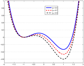
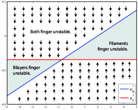
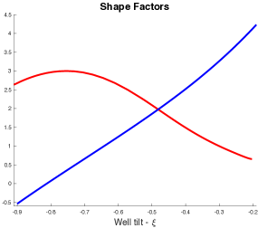
Figure 3: (left) Graph of the double well, $W$ versus $u$ for $\xi=-0.9,-0.7,-0.5$ (see (4.9)). (center) Diagram of the curve shortening regions in $\eta_{d}-\mu_{1}$ plane, for $\xi=-0.9$ and $\eta_{1}=0.15$. Arrows indicate the direction of the temporal evolution of $\mu_{1}$ under the flow (1.9). The shaded region is forward invariant and globally attracting so long as the curves remain admissible. (right) Values of the bilayer and filament shape factors, $S_{b}$ (blue) and $S_{{\it f}}$ (red) as a function of the well tilt, $\xi$. The change in sign of $S_{b}$ near $\xi=-0.8$ flips the direction of the inequality in (4.5).

4.2 Analysis of competitive geometric evolution and bifurcation

The analysis presents a bifurcation diagram with four thresholds that delineate distinct behaviors. The $\mu_{1}$ thresholds for the pearling bifurcation, $P_{b}$ and $P_{{\it f}}$, depend upon the functionalization parameters $\eta_{1}$ and $\eta_{2}$ through their difference $\eta_{d}:=\eta_{1}-\eta_{2}.$ The $\mu_{1}$ thresholds for the transition from curve shortening to regularized curve lengthening, $\mu_{b}^{*}$ and $\mu_{{\it f}}^{*}$ given in (2.52) and (3.81) respectively, have a more subtle dependence upon the functionalization parameters. These relations are summarized below:

$$\mu_{1}\,\textrm{sign}(S_{b})<P_{b}(\eta_{d}) :=-\eta_{d}\frac{\lambda_{b,0}\|\psi_{b,0}\|_{L^{2}}^{2}}{|S_{b}|},$$ Bilayers Pearling Stable (4.5)

$$\mu_{1}\,\textrm{sign}(S_{{\it f}})<P_{{\it f}}(\eta_{d}) :=-\eta_{d}\frac{\|\psi_{{{\it f}},0,0}^{\prime}\|_{L^{2}_{R}}^{2}+\lambda_{{{\it f}},0,0}\|\psi_{{{\it f}},0,0}\|^{2}_{L^{2}_{R}}}{|S_{f}|},$$ Filaments Pearling Stable (4.6)

$$\mu_{1}<\mu_{b}^{*}(\eta_{1},\eta_{2}),$$ Bilayers Curve Shortening (4.7)

$$\mu_{1}<\mu_{{\it f}}^{*}(\eta_{1},\eta_{2}), \textrm{Filament Curve Shortening}.$$ (4.8)

The signs of the shape factors $S_{b}$ and $S_{{\it f}}$, defined in (1.6), depend upon the choice of the double well, $W$, and impact not only the sign of the right-hand sides of (4.5) and (4.6) but also the direction of the inequalities, see Figure 3 (right). The chemical potential and the geometric flows evolve on the same $t=O(\varepsilon^{-1})$ timescale. Within the $H^{-1}$ gradient flow, the pearling instability produces eigenvalues of size $O(\varepsilon^{-1})$, [18] and hence will manifest itself on the $t=O(\varepsilon)$ timescale, essentially instantaneously on the time scale of the geometric flow and the chemical potential. We define the pearling instability region to be set of values $(\mu_{1},\eta_{1},\eta_{2})$ for which either codimension one or codimension two structures are pearling unstable.

We investigate the variation of the pearling instability regions, and its relation to regions of curve lengthening flows, as functions of the well shape. For simplicity we present these regions in the $\mu_{1}-\eta_{d}$ plane, with the assumption that $\eta_{1}=0.15$, unless specified otherwise. To parameterize the well shape we fix $b_{\pm}=\pm 1$ and insert a one-parameter well tilt, $\xi$ into the double-well potential,

$$W(u;\xi):=\frac{1}{2}(u-b_{-})^{2}\left(\frac{1}{2}(u-b_{+})^{2}-\frac{\xi}{3}\left(u-\frac{3b_{+}-b_{-}}{2}\right)\right),$$ (4.9)

where the parameter $\xi$ controls the value of $W$ at the right well $u=b_{+}$, see Figure 3 (left).

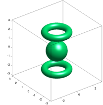
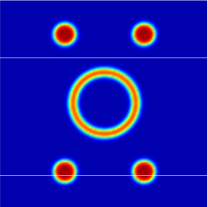
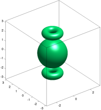
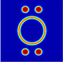
(a) $t=0$	(b) $t=0$ slice	(c) $t=200$	(d) $t=200$ slice

Figure 4: Simulation of the FCH gradient flow for $\varepsilon=0.03$, $\eta_{1}=0.15$, $\eta_{2}=0.24$, and $\xi=-0.15$. For these values $\mu_{b}^{*}<0<\mu_{{\it f}}^{*}$ and after a short transient bilayers will grow while filaments shrink. (a) Initial data consisting of two circular filaments and a spherical bilayer inside the $[-\pi,\pi]^{3}$ computational domain. (b) 2D slice along $x-z$ plane ($y=0$) of initial data. (c) 3D pose of the $t=200$ $(\tau=6)$ final computation stage and (d) corresponding 2D slice showing the larger bilayer and smaller filament radii.

For the $\mu_{1}$ dynamics, as $\eta_{1}$ and $\eta_{2}$ are fixed parameters, the temporal evolution of $\mu_{1}$ traces a vertical line segment on the diagram, with $\mu_{1}$ decreasing if it is larger than both $\mu_{b}^{*}$ and $\mu_{{\it f}}^{*}$ and increasing if it is smaller than both. The $\mu_{1}$-region bounded by the points $\{\mu_{b}^{*},\mu_{{\it f}}^{*}\}$ is attracting and forward invariant under the flow see Figure 3 (center). Within this invariant region the direction of the flow depends upon the overall curvatures of the two classes of morphologies; however to leading order the total area/length of the codimensional structures with the larger equilibrium value decreases monotonically and the other increases monotonically, so long as the morphologies remain admissible. A simulation of the FCH gradient flow with one spherical bilayer and two circular filaments is presented in Figure 4 for parameter values for which $\mu_{b}^{*}<\mu_{{\it f}}^{*}$.

Motivated by this example, and to further illustrate the dynamics, we consider a composite morphology consisting of $N_{b}$ spherical bilayers of radii $R_{1},\ldots,R_{N_{b}}$ and $N_{{\it f}}=O(\varepsilon^{-1})$ circular filaments of radii $r_{1},\ldots,r_{N_{{\it f}}}$. 1 For these special shapes the competitive evolution (1.7)-(1.9) reduces to

$$\dot{R}_{i} =\nu_{b}\left(\mu_{1}-\mu_{b}^{*}\right)\frac{2}{R_{i}},\hskip 36.135pti=1,\ldots,N_{b},$$ (4.10)

$$\dot{r}_{j} =\nu_{{\it f}}\left(\mu_{1}-\mu_{{\it f}}^{*}\right)\frac{1}{r_{j}},\hskip 36.135ptj=1,\ldots,\varepsilon^{-1}N_{{\it f}},$$ (4.11)

$$\dot{\mu}_{1} =-\frac{\alpha_{-}^{2}}{|\Omega|}\left(16\pi m_{b}\nu_{b}(\mu_{1}-\mu_{b}^{*})N_{b}+\varepsilon 4\pi^{2}m_{{\it f}}\nu_{f}(\mu_{1}-\mu_{f}^{*})\sum\limits_{j=1}^{N_{{\it f}}}\frac{1}{r_{j}}\right),$$ (4.12)

where the dot notation denotes differentiation with respect to $\tau=t/\varepsilon.$ The $\mu_{1}$ evolution depends upon the spherical bilayers only through their total number. Consistent with the discussion above, the bulk chemical potential $\mu_{1}$ decreases if $\mu_{1}>\max\{\mu_{b}^{*},\mu_{{{\it f}}}^{*}\}$ and increases if $\mu_{1}<\min\{\mu_{b}^{*},\mu_{{{\it f}}}^{*}\}$. The radii shrink or grow depending upon the signs of $\mu_{1}-\mu_{b}^{*}$ and $\mu_{1}-\mu_{{\it f}}^{*}$. If both $N_{b}$ and $N_{{\it f}}$ are positive, and $\mu_{b}^{*}\neq\mu_{{\it f}}^{*}$ then the system has no equilibrium. Assuming for simplicity of presentation that $\mu_{b}^{*}<\mu_{{\it f}}^{*}$, then after a possible transient the system enters a regime in which all spheres are growing and all circular filaments are shrinking. The radii $r_{j}$ will then decrease to zero in finite time due to the inverse relation between $\dot{r}_{j}$ and $r_{j}$. If the zero radius filaments are removed from the system and the remaining filaments re-indexed, then after a transient the set of hoops will be empty ($N_{{\it f}}=0$) and only spheres will remain. At this point $\mu_{1}$ will relax (quench) at an exponential rate from above to $\mu_{b}^{*}$ as the spherical radii grow, albeit at an exponentially decreasing rate as $\mu_{1}$ quenches to $\mu_{b}^{*}$. The equilibrium will be a collection of spherical bilayers of differing radii. We emphasize that in the growing regime spherical shapes are unstable to perturbation under the full flow (1.7). Manifestation of this instability requires sufficiently large values of $\nu_{b}(\mu_{1}-\mu_{b}^{*})>0$ in relation to the coefficient $\varepsilon k_{b}$ of the surface diffusion term in (1.7), and is triggered more easily with increasing radius. However, if the non-spherical excursions are not so large as to induce self-intersection, then the shapes return to spherical as $\mu_{1}$ quenches to $\mu_{b}^{*}$. Figure 5 presents a simulation of the full FCH gradient flow that illustrates this phenomena, while a rigorous derivation of the transient instability regime of the curve lengthening flow in $1+2D$ for nearly circular bilayers is presented in [5].

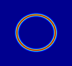
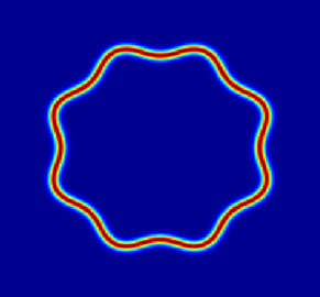
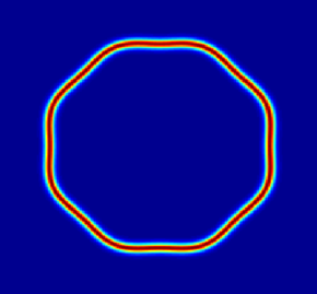
(a) $t=0$	(b) $t=484$	(c) $t=986$

Figure 5: Simulation of the FCH gradient flow corresponding to a single circular bilayer in $[-2\pi,2\pi]^{2}\subset\mathbb{R}^{2}$ in the regularized curve lengthening regime. The larger radii and value of $\mu_{1}-\mu_{b}^{*}$, compared to simulations presented in Figure 4, induce the interfacial meander. Yet larger initial values of $\mu_{1}-\mu_{b}^{*}$ lead to self-intersection and defect generation. (a) The initial data has $\mu_{1}>\mu_{b}^{*}$, with sufficient excess to initiate shape perturbations as the circular bilayer grows. (b) The onset of the shape instability at time $t=484$. (c) Quenching of the flow at $t=986$ as the value of $\mu_{1}$ relaxes towards $\mu_{b}*$ and the higher order surface diffusion returns the interface back to a larger, circular shape.

In Figure 6, the pearling bifurcation lines are added and the full stability diagram is shown for values of the well-tilt parameter $\xi=-0.85,-0.7,-0.45,$ and $-0.2$. For $\xi=-0.85$, $S_{{\it f}}$ is positive, $S_{b}$ is slightly negative, and for positive values of $\mu_{1}$ filament pearling instability region contains the bilayer pearling instability region. As $\xi$ is decreased from $-0.7$ to $-0.45$ the two pearling instability lines almost coincide, and for $\xi=-0.2$ they have crossed, with the filament pearling instability region now lying above the bilayer pearling instability region for $\mu_{1}>0$. In all figures the intersections of the pearling instability lines occurs to the left of the crossing of the curve lengthening lines. This implies that increasing $\eta_{d}$ from negative values will excite pearling bifurcations at smaller values of $\eta_{d}$ than those for which the filament morphology becomes dynamically favored over the bilayer morphology. For the non-generic value of $\eta_{d}$ at which the critical values $\mu_{b}^{*}=\mu_{{\it f}}^{*}$ coincide, codimension one and two structures can co-exist on the $t=O(\varepsilon^{-1})$ time-scales under consideration here.

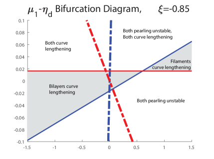
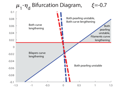
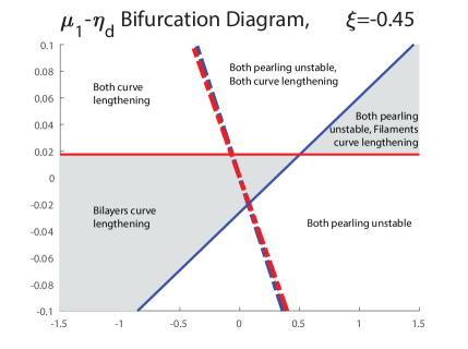
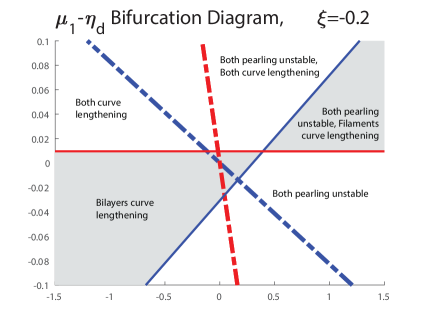
Figure 6: A $\mu_{1}\!-\!\,\eta_{d}$ bifurcation diagram versus $\mu_{1}$ (vertical axis) and $\eta_{d}$ (horizontal axis) for $\xi=-0.85,-0.7,-0.45$ and $-0.2$ and $\eta_{1}$ fixed at $\eta_{1}=0.15$. Pearling instability holds to the right of the dotted lines (blue-bilayers, red-filaments) while regularized curve lengthening holds above the solid lines (blue-bilayers, red-filaments). Areas of pearling instability and curve lengthening are indicated in key regions. The value of $\mu_{1}$ is generically time dependent, and the grey shaded region is forward invariant under the flow.

4.3 Analytic bifurcation diagrams and comparison to simulations

We compare the evolution of numerical simulations of the $H^{-1}$ gradient flow of the FCH free energy, (1.3), to the corresponding bifurcation results and to simulations from a self-consistent mean field model. The parameters impacting stability are the functionalization parameters $\eta_{1}$ and $\eta_{2}$, the time-dependent scaled chemical potential $\mu_{1}$, and the shape of the double well, parameterized by $\xi.$ For simplicity we fix $\eta_{1}=0.15$ and vary $\eta_{2}$ and $\xi$. Simulations of the strong FCH gradient flow, (1.1), were conducted in a domain $\Omega=[-\pi,\pi]^{3}\subset\mathbb{R}^{3}$, with initial data of the form (4.2) with $\Gamma_{b}$ consisting of a single sphere of radius $R_{1}=1.1$ with center at $(0,0,0)$ and $\Gamma_{{\it f}}$ comprised of two circular filaments of radius $r_{1}=r_{2}=1.6$ oriented parallel to the $x-y$ plain of $\Omega$ and with center point at $\left(0,0,\pm\frac{1}{2}(\pi+R_{1}/2)\right).$ The initial value of $\mu_{1}$ varied with each simulation and is reported in Figure 7. The system parameters are $\varepsilon=0.03$, $\eta_{1}=0.15$ and $\eta_{2}=0.24$, hence $\eta_{d}=-0.09$, and four separate values of $\xi:=-0.15,-0.2,-0.25,-0.3.$ In addition, there was one simulation for $\xi=-0.2$ and $\eta_{1}=\eta_{2}=0.15.$ The simulations were conducted for $t\in[0,100]$, equivalently $\tau\in[0,3]$.

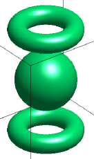
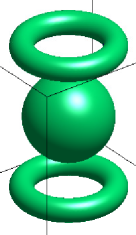
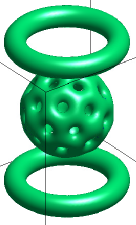
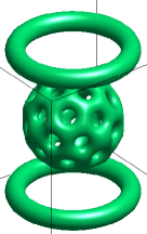
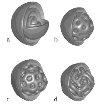
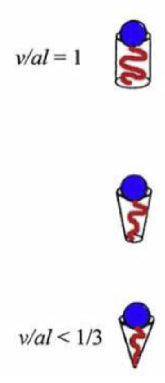
Figure 7: (left) The $t=100$ ($\tau=3$) end state of simulations of the FCH gradient flow for $\varepsilon=0.03$, $\eta_{1}=0.15$, $\eta_{2}=0.24$ from initial data described in the text and well tilt $\xi=-0.15,-0.20$ (top row, left to right), $\xi=-0.25,-0.3$ (bottom row, left to right). The less negative values of $\xi$ have initial values of $\mu_{1}$ that inhibit pearling, for the more negative two values the bilayer pearls. Images courtesy of Andrew Christlieb and Jaylan Jones. (center) Simulations of a mean-field density functional model of amphiphillic diblock copolymers with ratio of amphiphilic component of the diblock decreasing from (a) 35% (b) 30% (c) 25% (d) 20%. The minority solvent-hydrophilic phase is imaged. Reprinted (adapted) with permission from [13]. Copyright 2003 American Chemical Society. (right) Depiction of aspect ratio of lipids, a biological diblock with a short amphiphilic head and a long hydrophobic tail. The aspect ratio is defined as the lipid volume $v$ divided by the head cross-sectional area $a$ and tail length $l$. From [19], reprinted with permission from the Wiley publication. Copyright ©2011 WILEY-VCH Verlag GmbH & Co. KGaA, Weinheim.

Results for the five simulations are superimposed upon the corresponding $\mu_{1}\!-\!\eta_{d}$ bifurcation diagram and presented in Figure 8. The initial and final values of $\mu_{1}$ for each simulation are indicated with a closed circle and closed square respectively in each of the four diagrams. For $\xi=-0.15$ the value of $\mu_{1}$ starts in a region of bilayer and filament pearling stability, filament curve shortening, and bilayer regularized curve lengthening, see Figure 8(bottom-right). During the simulation the bilayer radius grew, the filaments shrunk, and neither pearled, the $\tau=3$ end state is presented in Figure 7 (left/top-left). Two simulations were conducted for $\xi=-0.2$, for the simulation with $\eta_{d}=-0.09$ the initial value of $\mu_{1}$ lies at the boarder of the bilayer pearling region, and the initial stages of the simulation $(t<5)$ displayed the onset of pearling, however the value of $\mu_{1}$ decreased out of the pearling region as the filaments and bilayers grow and the pearling evanesced, restoring the unpearled bilayer structure. The end-state is presented in Figure 7 (left/top-right), there is less shrinking of the circular filaments than in the case $\eta_{2}=-0.15$ and the filaments are thinner due to the stronger well tilt. The $\xi=-0.2$ simulation with $\eta_{d}=0$ but an identical initial value of $\mu_{1}$ starts in the middle of the bilayer pearling region, the bilayer pearled fully (end-state not shown) and the value of $\mu_{1}$ increased, see Figure 8 (bottom-left). The simulations with $\xi=-0.25$ and $\xi=-0.3$ begin within the bilayer pearling region, see Figure 8 (top-left and top-right) and rapidly pearled with the $\xi=-0.25$ simulation pearling around $t=5$ and the $\xi=-0.3$ simulation fully pearled at the first output time of $t=1$. The pearling leads to an increase in $\mu_{1}$ as the bilayer sheds net amphiphilic molecule mass to the bulk (far-field). The end states are depicted in Figure 7 (left/bottom-left and bottom-right).

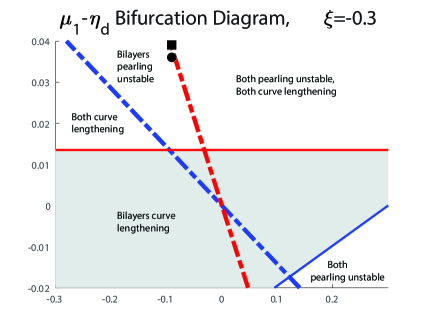
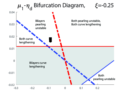
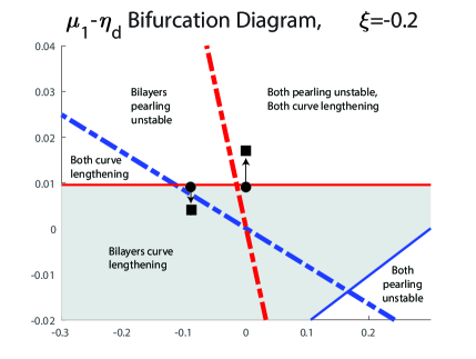
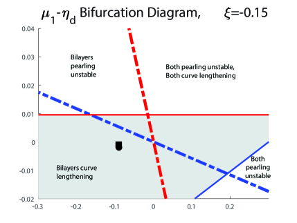
Figure 8: $\mu_{1}\!-\!\eta_{d}$ bifurcation diagrams with $\eta_{1}=0.15$ for the same values of $\xi$ as in the end-states depicted in Figure 7 (left). For the five simulations the initial and $t=100$ final value of $\mu_{1}$ is indicated on the corresponding bifurcation diagram with a solid black circle and square, respectively. The simulations with $\xi=-0.25,-0.3$ and $\xi=-0.2$ with $\eta_{d}=0$ lead to pearled morphologies.

The bilayer pearling instability was observed by Fraaije and Sevink, who developed a self-consistent mean field density functional model describing the free energy of amphiphilic diblock polymer surfactants embedded in solvent. Their model parameters are based upon poly(propylene oxide)-poly(ethylene oxide) diblock in an aqueous solution, see [13] and reference therein. They simulated spherical nanodroplets of 15% solvent and 85% polymer by volume. By decreasing the block ratio – the ratio of the length of the hydrophilic portion of the diblock chain to the length of the hydrophobic portion, they uncovered a series of bifurcations that lead from stable bilayers, to pearled bilayers to a continuous filament pattern decorated with $Y$-junctions and endcap defects, see Figure 7 (center). This change in block ratio from $35$% amphiphilic polymer down to $20$% amphiphilic polymer increases the aspect ratio of the minority phase. Within the context of the FCH, the parameter $\eta_{2}$ weighs the energy requirement of compressing the minority phase into the restricted core of a higher codimensional structure, corresponding to values of $u$ for which the double well $W$ is negative. In particular, bilayer profiles reside in the positive region of the double well, $W(\phi_{b})>0$, while the filament profile accesses the negative regions of $W$, consequently negative values of $\eta_{2}$ lower the energy cost of filaments relative to bilayers. In this sense positive values of $\eta_{2}$ penalize higher codimensional structures, which is analogous to amphiphilic molecule aspect ratio near one, while negative values of $\eta_{2}$ favor the packing found in high codimension morphologies, analogous to a high aspect ratio amphiphilic molecule, see Figure 7 (right). These preferences are born out in Figure 6: for fixed values of $\mu_{1}$, decreasing $\eta_{2}$ under constant $\eta_{1}$, hence increasing $\eta_{d}$, results in a crossing of the pearling stability line, leading to the pearled morphology seen in Figure 7 (center/b and c). Further increase in $\eta_{d}$ leads to a defect laden filament structure, see Figure 7 (center/d) consistent with slight crossing of the filament pearling stability line. This sequence, bilayer stability followed by bilayer pearling and then filament pearling for $\mu_{1}>0$ and increasing $\eta_{d}$ is consistent with a value of $\xi$ in the range $[-0.4,-0.2]$ depicted in Figure 6. The qualitative agreement between the pearled morphologies observed in the FCH free energy and the self-consistent density-functional model is striking. Both models present emergent pearling with smaller, round holes, compare Figure 7 (left/bottom-left) and (center/b), while fully emerged pearling leads to larger, pentagonal shaped holes, compare Figure 7 (left/bottom-right) and (center/c).

4.4 Comparison of analytical bifurcation diagrams to experiments

We compare the bifurcation structure derived for codimension 1 and 2 composite morphologies within the FCH gradient flow to experimental results of Dicher and Eisenberg reprinted in Figure 9 and of Jain and Bates reprinted in Figure 1.

4.4.1 Bifurcations of Dicher and Eisenberg

The bifurcation experiments of Dicher and Eisenberg, [10], depicted in Figure 1 (left), characterize the end-states of casts of PS-PAA amphiphilic diblocks dispersed in a water-dioxane solvent blend. Dioxane is a good solvent for both PEO and PS, but PS, like its commercial relative styrofoam, is strongly hydrophobic in water. Increasing the water content from zero leads to end-state morphologies, in order: solvability, only micelles, micelles and rods, only rods, rods and vesicles, and only vesicles. Here micelles are codimension 3, while rods and vesicles refer to codimension 2 and 1 respectively. An increase in water content in the solvent is analogous to an increase in $\eta_{1}$ – the energy release per unit of interface formation, under constant diblock aspect ratio, hence constant $\eta_{2}.$ This morphological bifurcation sequence can be emulated within the FCH equation by fixing $\xi=-0.5$ and $\eta_{2}=-0.4$ and allowing $\eta_{1}$ to vary from $0$ to $0.4$. The resulting $\mu_{1}\!-\!\,\eta_{1}$ bifurcation diagram is presented in Figure 9 (left). The curve shortening lines are presented within the view, the pearling stability lines are outside the view. For small values of $\eta_{1}$ filaments are dynamically favored, while bilayers are dynamically favored for larger values of $\eta_{1}$. In particular, the horizontal line is color coded to depict a probable end-state morphology of initial data consisting of an admissible composite solution with $\mu_{1}=0.05$. Here red denotes a pure filament end-state, blue a pure bilayer end-state and the yellow corresponds to a region of long-time coexistence of the two morphologies due to the approximate equality of the critical values $\mu_{b}^{*}=\mu_{{\it f}}^{*}$ for $\eta_{1}=0.22.$ However the bifurcation diagram lies within the pearling instability region of both bilayers and filaments, and as a result the FCH predicts that neither of these pure states would persist. This is a limitation in the FCH model, with the well choice considered here the intersection of the pearling bifurcation curves occurs at smaller values of $\eta_{1}$ than the intersection of the curve shortening lines. Agreement with these experimental results requires a robust inhibition of the pearling mechanism. Indeed, the experimental dynamics for the PS-PAA polymers considered here are largely reversible, as shown in Figure 9 (right), increasing and then decreasing the water content leads to a fully reversible sequence of morphological bifurcations. The presence of the pearling bifurcation generates complex morphologies with strong hysteresis, see Figure 10 (center). Matching this class of morphological bifurcation diagrams requires a tuning mechanism within the well shape $W$ that affords robust pearling inhibition. Such a mechanism is proposed within the context of multicomponent models in [23] and [12].

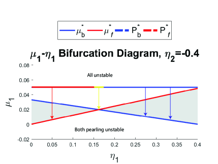
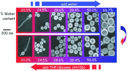
Figure 9: (left) A $\mu_{1}\!-\!\,\eta_{1}$ bifurcation diagram with $\xi=-0.5$ and $\eta_{2}=-0.4$ that shows the curve shortening lines for bilayers and filaments and vertical arrows showing generic evolution of $\mu_{1}$ from initial data starting at $0.05$ for $\eta_{1}$ running from $0$ to $0.4$. The color coding of the $\mu_{1}=0.05$ line indicates the final result of the end state with red denoting pure filament, yellow coexistence of filament and bilayer, and blue denoting pure bilayer; compare to Figure 1 (left) for increasing values of water in solvent phase. (right) Complete reversibility in a PS-PAA system under change in water solvent concentration, implying robust inhibition of pearling instabilities. From [10]. Reprinted with permission from AAAS.

4.4.2 Bifurcations of Jain and Bates

The experimental bifurcation diagram of Jain and Bates [16], depicted in Figure 1 (right), shows the end-state morphology of dispersions of PEO-PB with different polymer lengths and different weight fractions of PEO, $w_{\rm PEO}$, and hence different aspect ratios of the overall amphiphilic diblock. For comparison Figure 10 (left) depicts the end states of the FCH gradient flow corresponding to values of $\xi=-0.2$ and $\eta_{1}=0.15$ for initial values of $\mu_{1}=0.075$ and various values of $\eta_{d}$ arising from variation in $\eta_{2}$ which models the changes in diblock aspect ratio. Small, negative values of $\eta_{2}$ correspond to low values of $w_{\rm PEO}$ while larger, positives values of $\eta_{2}$ correspond to larger values of $w_{\rm PEO}$ and to negative values of $\eta_{d}$. The horizontal line in Figure 10 (left) is color coded to depict a probable end-state of the FCH evolution starting from an admissible composite solution with this value of $\mu_{1}$. On the left where $\eta_{d}<-0.5$, an initial value of $\mu_{1}=0.075$, both codimension one and two morphologies are in their curve lengthening region and both would increase in surface area/length. However as $\mu_{1}$ is depleted, the suspension enters the curve shortening region for filaments, which will either vanish in finite time or pearl as $\mu_{1}$ crosses the red dotted line – the end result is a pure bilayer state – indicated by the blue color of the horizontal line for this value of $\eta_{d}$.

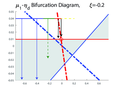
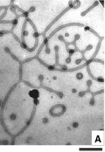
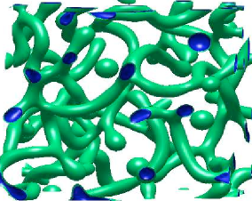
Figure 10: (left) A $\mu_{1}\!-\!\,\eta_{d}$ bifurcation diagram for $\xi=-0.2$ and fixed $\eta_{1}=0.15$, showing the end states of initial data with $\mu_{1}=0.04$ and varying values of $\eta_{2}$, with color coding corresponding to probable end state: blue–bilayer, green–network and defect structure (morphological complexit), red–filament, dotted yellow–filament and micelle. Compare to experimental results of Figure 1(right) for $N_{PB}=170$, with increasing values of $w_{PEO}$ corresponding to decreasing values of $\eta_{2}$. (center) Experimentally observed network, end cap, and $Y$-junction morphologies corresponding to the $C_{Y}$ phase of the bifurcation diagram from Figure 1 (right). Scale bar is $200$nm, From [16]. Reprinted with permission from AAAS. (right) End state of simulation of FCH gradient flow corresponding to green arrow, coarsened from random initial data, courtesy of Zhengfu Xu.

We focus on the values of $\eta_{d}$ in $[-0.35,-0.05]$, for which the horizontal line is colored green, to indicate a region of morphological complexity. The initial data lies in the bilayer pearling region, but passes transiently through it to bilayer pearling stability region. Depending upon the form of the initial bilayer morphology they may either fully pearl and form filament networks, or persist as bilayers and then grow after the return to pearling stability. Filament networks formed from the pearling of a bilayer typically host many $Y$-junctions and end caps. The filament network will expand until $\mu_{1}$ crosses the red-solid filament curve shortening line, at this point any defect free filaments will shrink, although the presence of any end-caps and $Y$-junctions in a particular component will render its evolution unclear. This uncertainty is reflected in the dotted nature of the bottom half of the green vertical line. The end result of the evolution is strongly dependent upon the form of the initial data, and will be very hysteretic in this regime. The uncertainty in the evolution is consistent with co-existing bilayers, filament networks, $Y$-junctured filaments, and end-cap defects, see Figure 10 (center) for a depiction of the experimental morphology found in this regime and Figure 10 (right) for a corresponding end-state of simulation of the FCH gradient flow from random initial data.

For large values of $\eta_{d}$ the $\mu_{1}$ flow remains in the bilayer pearling instability region, the bilayers either will not form or will pearl and transform to filament networks with the end-result being a $Y$-juncture dominated filament network. The last prediction, for $\eta_{d}=-0.02$ corresponds to the triple intersection (red circle) of the descending $\mu_{1}$ line, the filament pearling (red-dotted), and curve shortening (red-solid) lines. The arrival of $\mu_{1}$ to the filament curve shortening line from above is consistent with a stable filament phase, but the emergent pearling bifurcation signals a transition to end-cap and micelle formation, and corresponds to the possible coexistence of filament and micelle phases. This transition from filament to filament-micelle is reflected in the dotted nature of the yellow $\mu_{1}$ horizontal line for $\eta_{d}>-0.02$. A final transition to a pure micelle stage is plausible but is outside the scope of our analysis. The overall trend depicted in Figure 10 (left) suggests increasing $\eta_{d}$ at fixed $\eta_{1}$ results in bilayers, bilayers mixed with defective filaments (end caps and $Y$-junctions), filaments, and filaments coexisting with micelles. This bifurcation sequence is in excellence qualitative agreement with the $N_{\rm PB}=170$ bifurcation sequence depicted in Figure 1 (right) as the PEO weight fraction $w_{\rm PEO}$ decreases from high values to low values, corresponding to decreasing $\eta_{2}$ and hence increasing $\eta_{d}$ subject to constant values of $\eta_{1}$.

The bifurcation sequence depicted in Figure 1 (right) for $N_{\rm PB}=45$ corresponds to a much shorter, stiffer diblock polymer. In this regime the network and defect-laden filament phase are not observed, rather increasing $w_{\rm PEO}$ weight fraction leads to the codimensional bifurcation sequence which leads from bilayers, to coexistence of bilayers and filaments, to filaments, to coexistence of filaments and micelles, and finally to micelles. While the general trend of the codimensional bifurcation sequence is supported by the competitive geometric motion and its bifurcations, as in Figure 9 (left), we reiterate that within the context of the scalar version of the FCH free energy presented herein, the pearling bifurcation cannot be fully suppressed.

5 Discussion

We have presented a multiscale analysis of the $H^{-1}$ gradient flow of the FCH free energy corresponding to initial data close to dressings of admissible codimension one (bilayer) and codimension two (filament) morphologies. We derived their curvature driven flow which couples to the evolving, spatially constant far-field chemical potential, $\mu_{1}.$ This flow is the basis of the morphological competition, which barring other bifurcations leads to an end state corresponding to the dynamically favored morphology with the lower critical value, $\mu_{b}^{*}$ or $\mu_{{\it f}}^{*}$, of the far field chemical potential. In particular we identify regimes in which the geometric flow leads to growth or evanescence of each phase through curve shortening or regularized curve lengthening. Combining the curve shortening/regularized curve lengthening bifurcation with the pearling bifurcation results allows a characterization of the evolution of defect-free connected components of bilayer and filament morphologies. Our analysis predicts that codimension one and two structures do not generically coexist on the long, $t=O(\varepsilon^{-1})$ time scale within the strong FCH gradient flow. Experimental results show transitions between distinct codimensional phases with relatively large margins of coexistence, however as remarked in the experimental literature, the transients associated to these experiments are long compared to experimental patience and transients required to achieve a single phase of codimensional morphology may require months to years, [17].

We compared the analytical bifurcation diagram to results from numerical simulations of the FCH gradient flow, to simulations of a self-consistent mean-field density functional model for amphiphilic polymers, and to three sets of experimental studies of amphiphilic polymers. We find that the self-consistent mean-field density functional model proposed in [13] predicts a bifurcation sequence of radial bilayers, pearled bilayers, and filaments with end-cap defects in strong qualitative agreement with the FCH bifurcation structure, in particular the structure of the pearled spherical bilayers computed by both models are in excellent agreement. The experimental bifurcation analysis of Jain and Bates, [16], was conducted at two polymer lengths, long polymers with $N_{\rm PB}=170$ and shorter ones with $N_{\rm PB}=45.$ We find strong qualitative agreement between the FCH bifurcation structure and the experimental results for the longer chains, with the FCH results suggesting that the development of morphological complexity could be produced in a region in which bilayer pearling and filament curve shortening bifurcations lie in close proximity, see section 4.4.2. The passage of the far-field chemical potential through these bifurcations engenders network morphologies with $Y$-junctions, end-caps, and stable pearled filaments. The analytical basis of the complexity suggests a mechanism for hysteresis: the passage through these sequences of bifurcations will not be readily reversed by a non-adiabatic return of the state variables.

The FCH model with the parameter choices presented herein does not qualitatively reproduce all of the experimental results. Both the solvent quality bifurcation experiments of Dicher and Eisenberg, [10] and the short polymer $N_{\rm PB}=45$ experiments of Jain and Bates do not show evidence of pearling bifurcations. Complex morphology is not exhibited, and Dicher and Eisenberg show that for their experimental parameters the morphology is remarkably reversible: hysteresis is not observed. However, the Dicher and Eisenberg experimental bifurcation structure is well described by the dynamical favoritism arising from the morphological competition. To match the full range of experimental results the FCH free energy needs a tunable mechanism to robustly inhibit the pearling bifurcation. These can be achieved in two ways. The first is physically motivated: pearling is a modulation of bilayer width, and shorter polymers are stiffer and lead to bilayers with a less compressible width. The compressibility of the bilayer is tunable through the slope of the well $W$ at the value $u$ at which the bilayer density is greatest, generically the second $W=0$ crossing. Tuning this slope to be large represents a stiffer diblock and may serve to inhibit the pearling mechanism. The second mechanism is mathematically motivated: the pearling bifurcation arises from a balance between the positive eigenvalue $\lambda_{b,0}$ of the linearization $L_{b,0}$, see (2.7) about the bilayer profile, and the negative eigenspace of the Laplace-Beltrami operator, $\Delta_{s}$. The balance cannot occur if the operator $L_{b,0}$ is non-self adjoint and whose positive real part spectrum have non-zero imaginary parts. This arrangement can be tuned and detuned within a multicomponent model, providing precisely the desired mechanism for robust pearling inhibition. This mechanism was discussed in section 5 of [23] and forms the basis of the study of the singularly perturbed systems in [12].

There remains a considerable amount to address within the family of FCH energies. While the FCH is at some level a phenomenological model with parameter values that are not directly tunable from first principles, the FCH parameter values can be fit to experiments, or subscale molecular simulations, much like Flory Huggins parameters. Nonetheless, fitting the full form of a complicated well $W$, especially for multicomponent models, may be challenging. Even within the simple model presented here, the role of micelles on morphological competition has not been addressed, and their stability, including their growth into dumbbells and end-caped filaments is a primary instabilty mode that leads adiabatically from a codimension three structure into a defective codimension two structures. As there are almost no analytical characterization of defect modes, the micelle to dumbbell instability is worthy of study on a purely mathematical basis.

References

- Alikakos et al., [1999] Alikakos, N., Bates, P., and Chen, X. (1999). Periodic traveling waves and locating oscillating patterns in multidimensional domains. Transactions of the American Mathematical Society, 351(7):2777–2805.
- Alikakos et al., [2000] Alikakos, N. D., Bates, P. W., Chen, X., and Fusco, G. (2000). Mullins-sekerka motion of small droplets on a fixed boundary. Journal of Geometric Analysis, 10(4):575–596.
- Andreussi et al., [2012] Andreussi, O., Dabo, I., and Marzari, N. (2012). Revised self-consistent continuum solvation in electronic-structure calculations. The Journal of Chemical Physics, 136(6):064102.
- Blanazs et al., [2009] Blanazs, A., Armes, S. P., and Ryan, A. J. (2009). Self-assembled block copolymer aggregates: from micelles to vesicles and their biological applications. Macromolecular rapid communications, 30(4-5):267–277.
- [5] Chen, Y. and Promislow, K. (Preprint). Regularized curve lengthening for the strong FCH flow.
- Cooke and Deserno, [2006] Cooke, I. R. and Deserno, M. (2006). Coupling between lipid shape and membrane curvature. Biophysical journal, 91(2):487–495.
- Dai and Promislow, [2013] Dai, S. and Promislow, K. (2013). Geometric evolution of bilayers under the functionalized Cahn–Hilliard equation. In Proceedings of the Royal Society of London A: Mathematical, Physical and Engineering Sciences, volume 469, page 20120505. The Royal Society.
- Dai and Promislow, [2015] Dai, S. and Promislow, K. (2015). Competitive geometric evolution of amphiphilic interfaces. SIAM Journal on Mathematical Analysis, 47(1):347–380.
- [9] Dai, S. and Promislow, K. (Preprint). Geometrically constrained minimizers in dispersions of strongly hydrophobic amphiphilic polymer.
- Discher and Eisenberg, [2002] Discher, D. E. and Eisenberg, A. (2002). Polymer vesicles. Science, 297(5583):967–973.
- Doelman et al., [2014] Doelman, A., Hayrapetyan, G., Promislow, K., and Wetton, B. (2014). Meander and pearling of single-curvature bilayer interfaces in the functionalized Cahn–Hilliard equation. SIAM Journal on Mathematical Analysis, 46(6):3640–3677.
- [12] Doelman, A., Promislow, K., and Veerman, F. (Preprint). Freeways, tollroads, and pearling inhibition in multicomponent functionalized systems.
- Fraaije and Sevink, [2003] Fraaije, J. and Sevink, G. (2003). Model for pattern formation in polymer surfactant nanodroplets. Macromolecules, 36(21):7891–7893.
- Gavish et al., [2011] Gavish, N., Hayrapetyan, G., Promislow, K., and Yang, L. (2011). Curvature driven flow of bi-layer interfaces. Physica D: Nonlinear Phenomena, 240(7):675–693.
- Hayrapetyan and Promislow, [2015] Hayrapetyan, G. and Promislow, K. (2015). Spectra of functionalized operators arising from hypersurfaces. Zeitschrift für angewandte Mathematik und Physik, 66(3):631–662.
- Jain and Bates, [2003] Jain, S. and Bates, F. S. (2003). On the origins of morphological complexity in block copolymer surfactants. Science, 300(5618):460–464.
- Jain and Bates, [2004] Jain, S. and Bates, F. S. (2004). Consequences of nonergodicity in aqueous binary peo-pb micellar dispersions. Macromolecules, 37(4):1511–1523.
- Kraitzman and Promislow, [2018] Kraitzman, N. and Promislow, K. (2018). Pearling bifurcations in the strong functionalized Cahn–Hilliard free energy. SIAM Journal on Mathematical Analysis, 50(3):3395–3426.
- Mouritsen, [2011] Mouritsen, O. G. (2011). Lipids, curvature, and nano-medicine. European journal of lipid science and technology, 113(10):1174–1187.
- Pego, [1989] Pego, R. L. (1989). Front migration in the nonlinear Cahn-Hilliard equation. Proceedings of the Royal Society of London. A. Mathematical and Physical Sciences, 422(1863):261–278.
- Promislow and Wetton, [2009] Promislow, K. and Wetton, B. (2009). PEM fuel cells: a mathematical overview. SIAM Journal on Applied Mathematics, 70(2):369–409.
- Promislow and Wu, [2015] Promislow, K. and Wu, Q. (2015). Existence of pearled patterns in the planar functionalized cahn–hilliard equation. Journal of Differential Equations, 259(7):3298–3343.
- Promislow and Wu, [2017] Promislow, K. and Wu, Q. (2017). Existence, bifurcation, and geometric evolution of quasi-bilayers in the multicomponent functionalized Cahn–Hilliard equation. Journal of mathematical biology, 75(2):443–489.
- Scherlis et al., [2006] Scherlis, D. A., Fattebert, J.-L., Gygi, F., Cococcioni, M., and Marzari, N. (2006). A unified electrostatic and cavitation model for first-principles molecular dynamics in solution. The Journal of Chemical Physics, 124(7):074103.
- Zhu et al., [2009] Zhu, J., Ferrer, N., and Hayward, R. C. (2009). Tuning the assembly of amphiphilic block copolymers through instabilities of solvent/water interfaces in the presence of aqueous surfactants. Soft Matter, 5(12):2471–2478.
- Zhu and Hayward, [2012] Zhu, J. and Hayward, R. C. (2012). Interfacial tension of evaporating emulsion droplets containing amphiphilic block copolymers: Effects of solvent and polymer composition. Journal of Colloid and Interface Science, 365(1):275–279.