A Large Dimensional Study of Regularized Discriminant Analysis

Abstract

In this paper, we conduct a large dimensional study of regularized discriminant analysis classifiers with its two popular variants known as regularized LDA and regularized QDA. The analysis is based on the assumption that the data samples are drawn from a Gaussian mixture model with different means and covariances and relies on tools from random matrix theory (RMT). We consider the regime in which both the data dimension and training size within each class tends to infinity with fixed ratio. Under mild assumptions, we show that the probability of misclassification converges to a deterministic quantity that describes in closed form the performance of these classifiers in terms of the class statistics as well as the problem dimension. The result allows for a better understanding of the underlying classification algorithms in terms of their performances in practical large but finite dimensions. Further exploitation of the results permits to optimally tune the regularization parameter with the aim of minimizing the probability of misclassification. The analysis is validated with numerical results involving synthetic as well as real data from the USPS dataset yielding a high accuracy in predicting the performances and hence making an interesting connection between theory and practice.

I Introduction

Linear Discriminant analysis (LDA) is an old concept that dates back to Fisher that generalizes the Fisher discriminant [2, 3]. Given two statistically defined datasets, or classes, the Fisher discriminant analysis is designed to maximize the ratio of the variance between classes to the variance within classes and is useful for both classification and dimensionality reduction [4, 5]. LDA, on the other hand, relying merely on the concept of model based classification [4], is conceived so that the misclassification rate is minimized under a Gaussian assumption for the data. Interestingly, both ideas lead to the same classifier when the data of both classes share the same covariance matrix. Maintaining the Gaussian assumption but considering the general case of distinct covariance matrices, quadratic discriminant analysis (QDA) becomes the optimal classifier in terms of the minimization of the misclassification rate when both statistical means and covariances of the classes are known.

In practice, these parameters are rarely given and only estimated based on training data. Assuming the number of training samples is high enough, QDA and LDA should remain asymptotically optimal. It is however often the case in practice that the data dimension is large, if not larger, than the number of observations. In such circumstances, the covariance matrix estimate becomes ill-conditioned or even non invertible, which leads to poor classification performance.

To overcome this difficulty, many techniques can be considered. One can resort to dimensionality reduction so as to embed the data in a low-dimensional space that retains most of the useful information from a classification point of view [6, 7]. This ensures a higher number of training samples than the effective data size. Questions as to which dimensions to be selected or to what extent dimension should be reduced remain open. Another alternative involves the regularized versions of LDA and QDA denoted, throughout this paper, by R-LDA and R-QDA [5, 8]. Both approaches constitute the main focus of the article.

There exist many works on the performance analysis of discriminant analysis classifiers. In [9], an exact analysis of QDA is made by relying on properties of Wishart matrices. This allows for exact expressions of the probability misclassification rate for all sample size $n$ and dimension $p$. This analysis is however only valid as long as $n\geq p$ . Generalizing this analysis to regularized versions is however beyond analytical reach. This motivated further studies to consider asymptotic regimes. In [10, 11] the authors consider the large $p$ asymptotics and observe that LDA and QDA fall short even when the exact covariance matrix is known. [10] thus proposed improved LDA and PCA that exploit sparsity assumptions on the statistical means and covariances, however not necessarily met in practice. This leads us to consider in the present work the double asymptotic regime in which both $p$ and $n$ tend to infinity with fixed ratio. This regime leverages results from random matrix theory [12, 13, 14, 15, 16]. For LDA analysis, this regime was first considered in [17] under the assumption of equal covariance matrices. It was extended to the analysis of R-LDA in [8] and to the Euclidean distance discriminant rule in [18]. To the best of the authors’ knowledge, the general case in which the covariances across classes are different was never treated. As shown in the course of the paper, a major difficulty for the analysis resides in choosing the assumptions governing the growth rate of means and covariances to avoid nontrivial asymptotic classification performances.

This motivates the present work. Particularly, we propose a large dimensional analysis of both R-LDA and R-QDA in the double asymptotic regime for general Gaussian assumptions. Precisely, under technical, yet mild, assumptions controlling the distances between the class means and covariances, we prove that the probability of misclassification converges to a non-trivial deterministic quantity that only depends on the class statistics as well as the ratio $p/n$. Interestingly, R-LDA and R-QDA require different growth regimes, reflecting a fundamental difference in the way they leverage the information about the means and covariances. Notably, R-QDA requires a minimal distance between class means of order $O(\sqrt{p})$ while R-LDA necessitates a difference in means of order $O(1)$. However, R-LDA does not seem to leverage the information about the distance in covariance matrices. The results of [8] are in particular recovered when the spectral norm of the difference of covariance matrices is small. These findings lead to insights into when LDA or QDA should be preferred in practical scenarios.

To sum up, our main results are as follows:

• Under mild assumptions, we establish the convergence of the misclassification rate for both R-LDA and R-QDA classifiers to a deterministic error as a function of the statistical parameters associated with each class.

• We design a consistent estimator for the misclassification rate for both R-LDA and R-QDA classifiers allowing for a pre-estimate of the optimal regularization parameter.

• We validate our theoretical findings on both synthetic and real data drawn from the USPS dataset and illustrate the good accuracy of our results in both settings.

The remainder is organized as follows. We give an overview of discriminant analysis for binary classification in Section II. The main results are presented in Section III, the proofs of which are deferred to the Appendix. In Section IV, we design a consistent estimator of the misclassification error rate. We validate our analysis for real data in Section V and conclude the article in Section VI.
Notations: Scalars, vectors and matrices are respectively denoted by non-boldface, boldface lowercase and boldface uppercase characters. $\mathbf{0}_{p\times n}$ and $\mathbf{1}_{p\times n}$ are respectively the matrix of zeros and ones of size $p\times n$, $\mathbf{I}_{p}$ denotes the $p\times p$ identity matrix. The notation $\|.\|$ stands for the Euclidean norm for vectors and the spectral norm for matrices. $\left(.\right)^{T}$, $\mathop{\rm tr}\left(.\right)$ and $|.|$ stands for the transpose, the trace and the determinant of a matrix respectively. For two functionals $f$ and $g$, we say that $f=O\left(g\right)$, if $\exists\>0<M<\infty$ such that $|f|\leq Mg$. $\mathbb{P}\left(.\right)$, $\to_{d}$, $\to_{prob.}$ and $\to_{a.s.}$ respectively denote the probability measure, the convergence in distribution, the convergence in probability and the almost sure convergence of random variables. $\Phi\left(.\right)$ denotes the cumulative density function (CDF) of the standard normal distribution, i.e. $\Phi\left(x\right)=\int_{-\infty}^{x}\frac{1}{\sqrt{2\pi}}e^{-\frac{t^{2}}{2}}dt$.

II Discriminant Analysis for Binary Classification

This paper studies binary discriminant analysis techniques which employs a discriminant rule to assign for an input data vector the class to which it most likely belongs. The discriminant rule is designed based on $n$ available training data with known class labels. In this paper, we consider the case in which a bayesian discriminant rule is employed. Hence, we assume that observations from class $\mathcal{C}_{i}$, $i\in\{0,1\}$ are independent and are sampled from a multivariate Gaussian distribution with mean $\bm{\mu}_{i}\in\mathbb{R}^{p\times 1}$ and non-negative covariance matrix $\mathbf{\Sigma}_{i}\in\mathbb{R}^{p\times p}$. Formally speaking, an observation vector $\mathbf{x}\in\mathbb{R}^{p\times p}$ is classified to $\mathcal{C}_{i}$, $i\in\{0,1\}$, if

$$\mathbf{x}=\bm{\mu}_{i}+\bm{\Sigma}_{i}^{1/2}\bm{z},\quad\bm{z}\sim\mathcal{N}\left(\mathbf{0},\mathbf{I}_{p}\right).$$ (1)

Let

$$\begin{split}&W^{QDA}\left(\mathbf{x}\right)=-\frac{1}{2}\log\frac{|\mathbf{\Sigma}_{0}|}{|\mathbf{\Sigma}_{1}|}-\frac{1}{2}{\bf x}^{T}\left(\mathbf{\Sigma}_{0}^{-1}-\mathbf{\Sigma}_{1}^{-1}\right){\bf x}\\ &+{\bf x}^{T}\mathbf{\Sigma}_{0}^{-1}\bm{\mu}_{0}-{\bf x}^{T}\mathbf{\Sigma}_{1}^{-1}\bm{\mu}_{1}-\frac{1}{2}\bm{\mu}_{0}^{T}\mathbf{\Sigma}_{0}^{-1}\bm{\mu}_{0}+\frac{1}{2}\bm{\mu}_{1}^{T}\mathbf{\Sigma}_{1}^{-1}\bm{\mu}_{1}\\ &-\log\frac{\pi_{1}}{\pi_{0}}.\end{split}$$ (2)

As stated in [19], for distinct covariance matrices $\mathbf{\Sigma}_{0}$ and $\mathbf{\Sigma}_{1}$, the discriminant rule is summarized as follows

$$\left\{\begin{matrix}\mathbf{x}\in\mathcal{C}_{0}&\>\quad\quad\quad\quad\textnormal{if}\quad W^{QDA}\left(\mathbf{x}\right)>0.\\ \mathbf{x}\in\mathcal{C}_{1}&\textnormal{otherwise}.\end{matrix}\right.$$ (3)

When the considered classes have the same covariance matrix, i.e., $\mathbf{\Sigma}_{0}=\mathbf{\Sigma}_{1}$, the discriminant function simplifies to [5, 4, 8]

$$W^{LDA}\left(\mathbf{x}\right)=\left(\mathbf{x}-\frac{\bm{\mu}_{0}+\bm{\mu}_{1}}{2}\right)^{T}\mathbf{\Sigma}^{-1}\left(\bm{\mu}_{0}-\bm{\mu}_{1}\right)-\log\frac{\pi_{1}}{\pi_{0}}.$$ (4)

Classification obeys hence the following rule:

$$\left\{\begin{matrix}\mathbf{x}\in\mathcal{C}_{0}&\>\quad\quad\quad\quad\text{if}\quad W^{LDA}\left(\mathbf{x}\right)>0\\ \mathbf{x}\in\mathcal{C}_{1}&\textnormal{otherwise}.\end{matrix}\right.$$ (5)

Since $W^{LDA}$ is linear in ${\bf x}$, the corresponding classification method is referred to as linear discriminant analysis. As can be seen from (3) and (5), the classification rules assume the knowedge of the class statistics, namely their associated covariance matrices and mean vectors. In practice, these statistics can be estimated using the available training data. As such, we assume that $n_{i}$, $i\in\{0,1\}$ independent training samples $\mathcal{T}_{0}=\left\{\mathbf{x}_{l}\in\mathcal{C}_{0}\right\}_{l=1}^{n_{0}}$ and $\mathcal{T}_{1}=\left\{\mathbf{x}_{l}\in\mathcal{C}_{1}\right\}_{l=n_{0}+1}^{n_{0}+n_{1}=n}$ are respectively available to estimate the mean and the covariance matrix of each class $i$. For that, we consider the following sample estimates

$$\hat{\bm{\mu}}_{i} =\frac{1}{n_{i}}\sum_{l\in\mathcal{T}_{i}}\mathbf{x}_{l},\quad i\in\{0,1\}$$

$$\widehat{\mathbf{\Sigma}}_{i} =\frac{1}{n_{i}-1}\sum_{l\in\mathcal{T}_{i}}\left(\mathbf{x}_{l}-\hat{\bm{\mu}}_{i}\right)\left(\mathbf{x}_{l}-\hat{\bm{\mu}}_{i}\right)^{T},\quad i\in\{0,1\}$$

$$\widehat{\mathbf{\Sigma}} =\frac{\left(n_{0}-1\right)\widehat{\mathbf{\Sigma}}_{0}+\left(n_{1}-1\right)\widehat{\mathbf{\Sigma}}_{1}}{n-2},$$

where $\widehat{\mathbf{\Sigma}}$ is the pooled sample covariance matrix for both classes. To avoid singularity issues when $n_{i}<p$, we use the ridge estimator of the inverse of the covariance matrix [5]

$$\mathbf{H} =\left(\mathbf{I}_{p}+\gamma\widehat{\mathbf{\Sigma}}\right)^{-1},$$ (6)

$$\mathbf{H}_{i} =\left(\mathbf{I}_{p}+\gamma\widehat{\mathbf{\Sigma}}_{i}\right)^{-1},\quad i\in\{0,1\}$$ (7)

where $\gamma>0$ is a regularization parameter. Replacing $\bm{\Sigma}^{-1}$ and $\bm{\Sigma}_{i}$ for $i\in\{0,1\}$ by (6) and (7) into (4) and (3), we obtain the following discriminant rules

$$\widehat{W}^{R-LDA}\left(\mathbf{x}\right)=\left(\mathbf{x}-\frac{\hat{\bm{\mu}}_{0}+\hat{\bm{\mu}}_{1}}{2}\right)^{T}\mathbf{H}\left(\hat{\bm{\mu}}_{0}-\hat{\bm{\mu}}_{1}\right)-\log\frac{\pi_{1}}{\pi_{0}}.$$ (8)

$$\begin{split}\widehat{W}^{R-QDA}\left(\mathbf{x}\right)&=\frac{1}{2}\log\frac{|{\bf H}_{0}|}{|{\bf H}_{1}|}-\frac{1}{2}\left({\bf x}-\hat{\bm{\mu}}_{0}\right)^{T}{\bf H}_{0}\left({\bf x}-\hat{\bm{\mu}}_{0}\right)\\ &+\frac{1}{2}\left({\bf x}-\hat{\bm{\mu}}_{1}\right)^{T}{\bf H}_{1}\left({\bf x}-\hat{\bm{\mu}}_{1}\right)-\log\frac{\pi_{1}}{\pi_{0}}.\end{split}$$ (9)

The corresponding classification methods will be denoted respectively by R-LDA and R-QDA. Conditioned on the training samples $\mathcal{T}_{i}$, $i\in\{0,1\}$, the classification errors associated with R-LDA and R-QDA when ${\bf x}$ belongs to class $\mathcal{C}_{i}$ are given by

$$\epsilon_{i}^{R-LDA} =\mathbb{P}\left[\left(-1\right)^{i}\widehat{W}^{R-LDA}\left(\mathbf{x}\right)<0\>|\mathbf{x}\in\mathcal{C}_{i},\mathcal{T}_{0},\mathcal{T}_{1}\right].$$ (10)

$$\epsilon_{i}^{R-QDA} =\mathbb{P}\left[\left(-1\right)^{i}\widehat{W}^{R-QDA}({\bf x})<0\>|\mathbf{x}\in\mathcal{C}_{i},\mathcal{T}_{0},\mathcal{T}_{1}\right].$$ (11)

The total classification errors are respectively given by

$$\epsilon^{R-LDA} =\pi_{0}\epsilon_{0}^{R-LDA}+\pi_{1}\epsilon_{1}^{R-LDA}.$$

$$\epsilon^{R-QDA} =\pi_{0}\epsilon_{0}^{R-QDA}+\pi_{1}\epsilon_{1}^{R-QDA}.$$

In the following, we propose to analyze the asymptotic classication errors of both R-LDA and R-QDA when $p,n_{i}$ grow large at the same rate. For R-LDA, our results cover a more general setting than the one studied in [8], in that they apply to the case where both classes have distinct covariance matrices.

III Main Results

The main contributions of the present work are two fold. First, we carry out an asymptotic analysis of the classification error rate for both R-LDA and R-QDA, showing that they converge to some deterministic quantities that depend solely on the observations statistics associated with each class. Such a result allows a better understanding of the impact of these parameters on the performances. Second, we build consistent estimates of the asymptotic misclassification error rates for both estimators. An estimator of the misclassification error rate has been provided in [8] but for the R-LDA when the classes are assumed to have identical covariance matrices. Our results regarding R-LDA in this respect extends the one in [8] when the covariance matrices are not equal. The treatment of R-QDA is however new and constitute the main contribution of the present work.

III-A Asymptotic Performance of R-LDA with Distinct Covariance Matrices

In this section, we present an asymptotic analysis of the R-LDA classifier. Our analysis is mainly based on recent results from RMT concerning some properties of Gram matrices of mixture models [16]. We recall that [8] made a similar analysis of R-LDA in the double asymptotic regime when both classes have a common covariance matrix, thereby not requiring these advanced tools. As such, our results can be viewed as a generalization of [8] when both classes have distinct covariance matrices. This permits to evaluate the performance of R-LDA in practical scenarios when the assumption of common covariance matrices cannot always be guaranteed. To allow derivations, we shall consider the following growth rate assumptions

Assumption. 1 (Data scaling).

$\frac{p}{n}\to c\in\left(0,\infty\right)$.

Assumption. 2 (Class scaling).

$\frac{n_{i}}{n}\to c_{i}\in\left(0,\infty\right)$, for $i\in\{0,1\}$.

Assumption. 3 (Covariance scaling).

$\lim\sup_{p}\left\|\mathbf{\Sigma}_{i}\right\|<\infty$, for $i\in\{0,1\}$.

Assumption. 4 (Mean scaling).

Let $\bm{\mu}=\bm{\mu}_{0}-\bm{\mu}_{1}$. Then, $\lim\sup_{p}\|\bm{\mu}\|=\lim\sup_{p}\|\bm{\mu}_{0}-\bm{\mu}_{1}\|<\infty$.

These assumptions are mainly considered to achieve an asymptotically non-trivial classification error. Assumption 3 is frequently met within the framework of random matrix theory [16]. Under the setting of Assumption 3, Assumption 4 ensures that a nontrivial classification rate is obtained: If $\left\|\bm{\mu}_{0}-\bm{\mu}_{1}\right\|$ scales faster than $O\left(1\right)$, then perfect asymptotic classification is achieved; however, if $\left\|\bm{\mu}_{0}-\bm{\mu}_{1}\right\|$ scales slower than $O\left(1\right)$, classification is asymptotically impossible. Assumptions 1 and 2 respectively control the growth rate in the data and the training.

III-A1 Deterministic Equivalent

We are in a position to derive a deterministic equivalent of the misclassification error rate of the R-LDA. Indeed, conditioned on the training data $\mathbf{x}_{1},\cdots,\mathbf{x}_{n}$, the probability of misclassification is given by: [8]

$$\epsilon^{R-LDA}_{i}=\Phi\left(\frac{\left(-1\right)^{i+1}G\left(\bm{\mu}_{i},\hat{\bm{\mu}}_{0},\hat{{\bm{\mu}}}_{1},\mathbf{H}\right)+\left(-1\right)^{i}\log\frac{\pi_{1}}{\pi_{0}}}{\sqrt{D\left({\hat{\bm{\mu}}}_{0},\hat{{\bm{\mu}}}_{1},\mathbf{H},\mathbf{\Sigma}_{i}\right)}}\right),$$ (12)

where

$$G\left(\bm{\mu}_{i},\hat{{\bm{\mu}}}_{0},\hat{{\bm{\mu}}}_{1},\mathbf{H}\right)=\left(\bm{\mu}_{i}-\frac{\hat{\bm{\mu}}_{0}+\hat{{\bm{\mu}}}_{1}}{2}\right)^{T}\mathbf{H}\left(\hat{{\bm{\mu}}}_{0}-\hat{{\bm{\mu}}}_{1}\right).$$ (13)

$$D\left(\hat{{\bm{\mu}}}_{0},\hat{{\bm{\mu}}}_{1},\mathbf{H},\mathbf{\Sigma}_{i}\right)=\left(\hat{{\bm{\mu}}}_{0}-\hat{{\bm{\mu}}}_{1}\right)^{T}\mathbf{H}\mathbf{\Sigma}_{i}\mathbf{H}\left(\hat{{\bm{\mu}}}_{0}-\hat{{\bm{\mu}}}_{1}\right).$$ (14)

The total misclassification probability is thus given by

$$\epsilon^{R-LDA}=\pi_{0}\epsilon^{R-LDA}_{0}+\pi_{1}\epsilon^{R-LDA}_{1}.$$ (15)

Prior to stating the main result concerning R-LDA, we shall introduce the following quantities, which naturally appear, as a result of applying [16]. Let $\bar{\mathbf{Q}}\left(z\right)$ be the matrix defined as follows

$$\bar{\mathbf{Q}}\left(z\right)\triangleq-\frac{1}{z}\left(\mathbf{I}_{p}+c_{0}g_{0}(z)\mathbf{\Sigma}_{0}+c_{1}g_{1}(z)\mathbf{\Sigma}_{1}\right)^{-1},\>z\in\mathbb{C}.$$ (16)

where $g_{i}(z)$, $i\in\{0,1\}$, satisfies the following fixed point equations

$$\frac{p}{n}g_{i}(z)=-\frac{1}{z}\frac{1}{1+\tilde{g}_{i}(z)},\>\>\tilde{g}_{i}(z)=\frac{1}{p}\mathop{\rm tr}\bm{\Sigma}_{i}\bar{\mathbf{Q}}\left(z\right).$$ (17)

Also define ${\bf A}_{i}=\bm{\Sigma}_{i}\bar{\bf Q}(z)$ and $\widetilde{\mathbf{Q}}_{i}\left(z\right)$ as

$$\widetilde{\mathbf{Q}}_{i}\left(z\right)\triangleq\bar{\bf Q}(z)\left({\bf A}_{i}+R_{0}{\bf A}_{0}+R_{1}{\bf A}_{1}\right),$$ (18)

where

$$R_{i}=\frac{z^{2}c_{i}g_{i}^{2}(z)\frac{1}{n}\mathop{\rm tr}{\bf A}_{0}{\bf A}_{1}}{1-\left(z^{2}c_{0}g_{0}^{2}(z)+z^{2}c_{1}g_{1}^{2}(z)\right)\frac{1}{n}\mathop{\rm tr}{\bf A}_{0}{\bf A}_{1}},\ \ i\in\left\{0,1\right\}.$$ (19)

The quantities in (17) can be computed in an iterative fashion where convergence is guaranteed after few iterations (see [16] for more details). Moreover, define

$$\overline{G}_{i}\left(z\right) \triangleq\frac{\left(-1\right)^{i+1}}{2}z\bm{\mu}^{T}\bar{\mathbf{Q}}\left(z\right)\bm{\mu}+\frac{z}{2n_{0}}\mathop{\rm tr}{\bf A}_{0}-\frac{z}{2n_{1}}\mathop{\rm tr}{\bf A}_{1}.$$ (20)

$$\overline{D}_{i}\left(z\right) \triangleq z^{2}\bm{\mu}^{T}\widetilde{\mathbf{Q}}_{i}\left(z\right)\bm{\mu}+\frac{z^{2}}{n_{0}}\mathop{\rm tr}\mathbf{\Sigma}_{0}\widetilde{\mathbf{Q}}_{i}\left(z\right)+\frac{z^{2}}{n_{1}}\mathop{\rm tr}\mathbf{\Sigma}_{1}\widetilde{\mathbf{Q}}_{i}\left(z\right),$$ (21)

where $\bm{\mu}=\bm{\mu}_{0}-\bm{\mu}_{1}$. With these definitions at hand, we state the following theorem

Theorem. 1.

Under Assumptions 1-4, we have

$$G\left(\bm{\mu}_{i},\hat{\bm{\mu}}_{0},\hat{\bm{\mu}}_{1},\mathbf{H}\right)-\overline{G}_{i}\left(-\frac{1}{c\gamma}\right) \to_{a.s.}0.$$ (22)

$$D\left(\hat{\bm{\mu}}_{0},\hat{\bm{\mu}}_{1},\mathbf{H},\mathbf{\Sigma}_{i}\right)-\overline{D}_{i}\left(-\frac{1}{c\gamma}\right) \to_{a.s.}0.$$ (23)

As a consequence, the conditional misclassification probability converges almost surely to a deterministic quantity $\bar{\epsilon}_{i}^{R-LDA}$

$$\epsilon_{i}^{R-LDA}-\bar{\epsilon}_{i}^{R-LDA}\to_{a.s.}0,$$ (24)

where

$$\bar{\epsilon}_{i}^{R-LDA}=\Phi\left(\frac{\left(-1\right)^{i+1}\overline{G}_{i}+\left(-1\right)^{i}\log\left(\frac{\pi_{0}}{\pi_{1}}\right)}{\sqrt{\overline{D}_{i}}}\right).$$ (25)

Proof.

See Appendix A. ∎

Remark. 1.

As stated earlier, if $\|\bm{\mu}\|$ scales faster than $O\left(1\right)$, perfect asymptotic classification is achieved. This can be seen by noticing that $\frac{\overline{G}_{i}\left(-\frac{1}{c\gamma}\right)}{\sqrt{\overline{D}_{i}\left(-\frac{1}{c\gamma}\right)}}$ would grow indefinitely large with $p$, thereby making the conditional error rates vanish.

When $\left\|\bm{\Sigma}_{0}-\bm{\Sigma}_{1}\right\|$ converges to zero, the asymptotic misclassification error rate of each class coincides with the one derived in [8] obtained when $\mathbf{\Sigma}_{0}=\mathbf{\Sigma}_{1}$.

Corollary. 1.

In the case where $\|\mathbf{\Sigma}_{0}-\mathbf{\Sigma}_{1}\|=o\left(1\right)$ (including the common covariance case where $\mathbf{\Sigma}_{0}=\mathbf{\Sigma}_{1}=\mathbf{\Sigma}$), the conditional misclassification error rate converges almost surely to $\overline{\overline{\epsilon}}_{i}^{R-LDA}$

$$\overline{\overline{\epsilon}}_{i}^{R-LDA}=\Phi\left(\frac{(-1)^{i+1}\overline{\overline{G}}_{i}(-\frac{1}{c\gamma})+(-1)^{i}\log\frac{\pi_{0}}{\pi_{1}}}{\sqrt{\overline{\overline{D}}_{i}(-\frac{1}{c\gamma})}}\right),$$

where

$$\overline{\overline{G}}_{i}\left(-\frac{1}{c\gamma}\right) =\frac{\left(-1\right)^{i}}{2}\bm{\mu}^{T}\left(\mathbf{I}_{p}+\frac{\gamma}{1+\gamma\delta}\mathbf{\Sigma}\right)^{-1}\bm{\mu}-\frac{n\delta}{2}\left(\frac{1}{n_{0}}-\frac{1}{n_{1}}\right)$$

$$\overline{\overline{D}}_{i}\left(-\frac{1}{c\gamma}\right)$$

$$=\frac{\left[\bm{\mu}^{T}\mathbf{\Sigma}\left(\mathbf{I}_{p}+\frac{\gamma}{1+\gamma\delta}\mathbf{\Sigma}\right)^{-2}\bm{\mu}+\left(\frac{1}{n_{0}}+\frac{1}{n_{1}}\right)\mathop{\rm tr}\mathbf{\Sigma}^{2}\left(\mathbf{I}_{p}+\frac{\gamma}{1+\gamma\delta}\mathbf{\Sigma}\right)^{-2}\right]}{1-\frac{\gamma^{2}}{n\left(1+\gamma\delta\right)^{2}}\mathop{\rm tr}\mathbf{\Sigma}^{2}\left(\mathbf{I}_{p}+\frac{\gamma}{1+\gamma\delta}\mathbf{\Sigma}\right)^{-2}}.$$

where $\bm{\Sigma}=\bm{\Sigma}_{0}$ or $\bm{\Sigma}=\bm{\Sigma}_{1}$, and $\delta$ is the unique positive solution to the following equation:

$$\delta=\frac{1}{n}\mathop{\rm tr}\bm{\Sigma}\left({\bf I}_{p}+\frac{\gamma}{1+\gamma\delta}\bm{\Sigma}\right)^{-1}.$$

Proof.

When $\|\mathbf{\Sigma}_{0}-\mathbf{\Sigma}_{1}\|=o\left(1\right)$, we first prove that up to an error $o(1)$, the key deterministic equivalents can be simplified to depend only on $\bm{\Sigma}_{0}$ (or $\mathbf{\Sigma}_{1}$). In the sequel, we take $\bm{\Sigma}=\bm{\Sigma}_{0}$. As $\|\mathbf{\Sigma}_{0}-\mathbf{\Sigma}_{1}\|=o\left(1\right)$, we have

$$\tilde{g}_{i}\left(z\right)=\underbrace{\frac{1}{p}\mathop{\rm tr}\mathbf{\Sigma}\bar{\mathbf{Q}}\left(z\right)}_{\tilde{g}\left(z\right)}+o(1),\>\forall i\in\{0,1\}.$$

It follows that $g_{i}\left(z\right)=g\left(z\right)+o(1)$ where $g\left(z\right)=-\frac{1}{z}\frac{n}{p}\frac{1}{1+\tilde{g}\left(z\right)}$. The above relations allow to simplify functionals involving matrix $\bar{\mathbf{Q}}$. To see that, we decompose $\bar{\mathbf{Q}}$ as

$$\bar{\mathbf{Q}}\left(z\right)$$

$$=-z^{-1}\left(\mathbf{I}+g\left(z\right)\mathbf{\Sigma}_{0}+c_{1}g\left(z\right)\left(\mathbf{\Sigma}_{1}-\mathbf{\Sigma}_{0}\right)\right)^{-1}+o_{\|.\|}(1)$$

$$=-z^{-1}\left(\mathbf{I}+g\left(z\right)\mathbf{\Sigma}_{0}\right)^{-1}-z^{-1}\Biggl{[}\left(\mathbf{I}+g\left(z\right)\mathbf{\Sigma}_{0}+c_{1}g\left(z\right)\left(\mathbf{\Sigma}_{1}-\mathbf{\Sigma}_{0}\right)\right)^{-1}$$

$$-\left(\mathbf{I}+g\left(z\right)\mathbf{\Sigma}_{0}\right)^{-1}\Biggr{]}+o_{\|.\|}(1)$$

$$\overset{(a)}{=}-z^{-1}\left(\mathbf{I}+g\left(z\right)\mathbf{\Sigma}_{0}\right)^{-1}$$

$$-z^{-1}\left(\mathbf{I}+g\left(z\right)\mathbf{\Sigma}_{0}+c_{1}g\left(z\right)\left(\mathbf{\Sigma}_{1}-\mathbf{\Sigma}_{0}\right)\right)^{-1}c_{1}g\left(z\right)\left(\mathbf{\Sigma}_{1}-\mathbf{\Sigma}_{0}\right)$$

$$\times\left(\mathbf{I}+g\left(z\right)\mathbf{\Sigma}_{0}\right)^{-1}+o_{\|.\|}(1)$$

where $(a)$ follows from the resolvent identity and $o_{\|.\|}(1)$ denotes a matrix with spectral norm converging to zero. Define

$$\mathbf{\Psi} =z^{-1}\left(\mathbf{I}+g\left(z\right)\mathbf{\Sigma}_{0}+c_{1}g\left(z\right)\left(\mathbf{\Sigma}_{1}-\mathbf{\Sigma}_{0}\right)\right)^{-1}c_{1}g\left(z\right)\left(\mathbf{\Sigma}_{1}-\mathbf{\Sigma}_{0}\right)$$

$$\times\left(\mathbf{I}+g\left(z\right)\mathbf{\Sigma}_{0}\right)^{-1}.$$

Then, it can be shown using the inequality $\|\mathbf{AB}\|\leq\|{\bf A}\|\|{\bf B}\|$ for ${\bf A}$ and ${\bf B}$ two matrices in $\mathbb{R}^{p\times p}$ that:

$$\|\mathbf{\Psi}\|\overset{(b)}{\leq}z^{-1}c_{1}g\left(z\right)\|\mathbf{\Sigma}_{0}-\mathbf{\Sigma}_{1}\|$$

$$\times\left\|\left(\mathbf{I}+g\left(z\right)\mathbf{\Sigma}_{0}+c_{1}g\left(z\right)\left(\mathbf{\Sigma}_{1}-\mathbf{\Sigma}_{0}\right)\right)^{-1}\left(\mathbf{I}+g\left(z\right)\mathbf{\Sigma}_{0}\right)^{-1}\right\|$$

$$=o\left(1\right).$$

Hence, for ${\bf a},{\bf b}\in\mathbb{R}^{p}$,

$$\bm{a}^{T}\bar{\mathbf{Q}}\left(z\right)\bm{b}=-z^{-1}\bm{a}^{T}\left(\mathbf{I}+g\left(z\right)\mathbf{\Sigma}\right)^{-1}\bm{b}+o(1),$$

and $\frac{1}{p}\mathop{\rm tr}{\bf A}\bar{\mathbf{Q}}=\frac{-z^{-1}}{p}\mathop{\rm tr}{\bf A}\left(\mathbf{I}+g\left(z\right)\mathbf{\Sigma}\right)^{-1}+o(1)$. Using the same notations as in [8] we have in particular for $z=-\frac{1}{c\gamma}$, $\tilde{g}\left(z\right)=\delta+o(1)$ and $g\left(z\right)=\frac{\gamma}{1+\gamma\delta}+o(1)$, where $\delta$ is the fixed-point solution in [8, Proposition 1]. Moreover,

$$\frac{z}{2n_{0}}\mathop{\rm tr}\mathbf{\Sigma}_{0}\bar{\mathbf{Q}}\left(z\right)-\frac{z}{2n_{1}}\mathop{\rm tr}\mathbf{\Sigma}_{1}\bar{\mathbf{Q}}\left(z\right)$$

$$=\frac{z\mathop{\rm tr}\mathbf{\Sigma}_{0}\bar{\mathbf{Q}}\left(z\right)}{2}\left(\frac{1}{n_{0}}-\frac{1}{n_{1}}\right)+\underbrace{\frac{z}{2n_{1}}\mathop{\rm tr}\left(\mathbf{\Sigma}_{0}-\mathbf{\Sigma}_{1}\right)\bar{\mathbf{Q}}\left(z\right)}_{\leq\|\mathbf{\Sigma}_{0}-\mathbf{\Sigma}_{1}\|\frac{z}{2n_{1}}\mathop{\rm tr}\bar{\mathbf{Q}}\left(z\right)}$$

$$=\frac{z\mathop{\rm tr}\mathbf{\Sigma}\bar{\mathbf{Q}}\left(z\right)}{2}\left(\frac{1}{n_{0}}-\frac{1}{n_{1}}\right)+o\left(1\right)$$

$$=\frac{-\mathop{\rm tr}\mathbf{\Sigma}\left(\mathbf{I}+g\left(z\right)\mathbf{\Sigma}\right)^{-1}}{2}\left(\frac{1}{n_{0}}-\frac{1}{n_{1}}\right)+o\left(1\right).$$

It follows that

$$\overline{G}_{i}\left(-\frac{1}{c\gamma}\right) =\frac{\left(-1\right)^{i}}{2}\bm{\mu}^{T}\left(\mathbf{I}_{p}+\frac{\gamma}{1+\gamma\delta}\mathbf{\Sigma}\right)^{-1}\bm{\mu}$$

$$-\frac{n\delta}{2}\left(\frac{1}{n_{0}}-\frac{1}{n_{1}}\right)+o\left(1\right).$$

Using the same arguments, we can show that

$$\overline{D}_{i}\left(-\frac{1}{c\gamma}\right)=\left[1-\frac{\gamma^{2}}{n\left(1+\gamma\delta\right)^{2}}\mathop{\rm tr}\mathbf{\Sigma}^{2}\left(\mathbf{I}_{p}+\frac{\gamma}{1+\gamma\delta}\mathbf{\Sigma}\right)^{-2}\right]^{-1}$$

$$\times\Biggl{[}\bm{\mu}^{T}\mathbf{\Sigma}\left(\mathbf{I}_{p}+\frac{\gamma}{1+\gamma\delta}\mathbf{\Sigma}\right)^{-2}\bm{\mu}$$

$$+\left(\frac{1}{n_{0}}+\frac{1}{n_{1}}\right)\mathop{\rm tr}\mathbf{\Sigma}^{2}\left(\mathbf{I}_{p}+\frac{\gamma}{1+\gamma\delta}\mathbf{\Sigma}\right)^{-2}\Biggr{]}+o(1).$$

∎

Corollary 1 is useful because it allows to specify the range of applications of Theorem 1 in which the information on the covariance matrix is essential for the classification task. Also, it shows how R-LDA is robust against small perturbations in the covariance matrix. Similar observations have been made in [20] where it was shown via a Monte Carlo study that LDA is robust against the modeling assumptions.

III-B Asymptotic Performance of R-QDA

In this part, we state the main results regarding the derivation of deterministic approximations of the R-QDA classification error. Such results have been obtained by considering some specific assumptions, carefully chosen such that an asymptotically non-trivial classification error (i.e., neither $0$ nor $1$) is achieved. We particularly highlight how the provided asymptotic approximations depend on such statistical parameters as the means and covariances within classes, thus allowing a better understanding of the performance of the R-QDA classifier. Ultimately, these results can be exploited in order to improve the performances by allowing optimal setting of the regularization parameter.

III-B1 Technical Assumptions

We consider the following double asymptotic regime in which $n_{i},$ $p$ $\to\infty$ for $i\in\{0,1\}$ with the following assumptions met

Assumption. 5 (Data scaling).

$n_{0}-n_{1}=o\left(1\right)$ and $\frac{p}{n}\to c\in\left(0,\infty\right)$.

Assumption. 6 (Mean scaling).

$\left\|\bm{\mu}_{0}-\bm{\mu}_{1}\right\|^{2}=O\left(\sqrt{p}\right)$.

Assumption. 7 (Covariance scaling).

$\left\|\mathbf{\Sigma}_{i}\right\|=O\left(1\right)$.

Assumption. 8.

Matrix $\bm{\Sigma}_{0}-\bm{\Sigma}_{1}$ has exactly $O(\sqrt{p})$ eigenvalues of order $O(1)$. The remaining eigenvalues are of order $O(\frac{1}{\sqrt{p}})$.

Assumption 5 implies also that $\pi_{i}\to\frac{1}{2}$ for $i\in\left\{0,1\right\}$. As we shall see later, if this is not satisfied, the R-QDA perform asymptotically as the classifier that assigns all observations to the same class. The second assumption governs the distance between the two classes in terms of the Euclidean distance between the means. This is mandatory in order to avoid asymptotic perfect classification. This is a much stronger assumption than Assumption 2 in R-LDA since we allow larger values for $\|\bm{\mu}_{0}-\bm{\mu}_{1}\|$. This can be understood as R-QDA being subject to strong noise induced when estimating $\mathbf{\Sigma}_{i}$, $i\in\{0,1\}$ which requires a large value $\|\bm{\mu}_{0}-\bm{\mu}_{1}\|$ so that it can play a role in classification. A similar assumption is required to control the distance between the covariance matrices. Particularly, the spectral norm of the covariance matrices are required to be bounded as stated in Assumption 7 while their difference should satisfy Assumption 8.The latter assumption implies that for any matrix ${\bf A}$ of bounded spectral norm,

$$\frac{1}{\sqrt{p}}\mathop{\rm tr}{\bf A}(\bm{\Sigma}_{0}-\bm{\Sigma}_{1})=O(1).$$

III-B2 Central Limit Theorem (CLT)

It can be easily shown that the R-QDA conditional classification error in (11) can be expressed as

$$\epsilon^{R-QDA}_{i}=\mathbb{P}\left[\bm{z}^{T}\mathbf{B}_{i}\bm{z}+2\bm{z}^{T}\mathbf{r}_{i}<\xi_{i}|\bm{z}\sim\mathcal{N}\left(\mathbf{0},\mathbf{I}_{p}\right),\mathcal{T}_{0},\mathcal{T}_{1}\right],$$ (26)

where

$$\mathbf{B}_{i} =\mathbf{\Sigma}_{i}^{1/2}\left(\mathbf{H}_{1}-\mathbf{H}_{0}\right)\mathbf{\Sigma}_{i}^{1/2},$$

$$\mathbf{r}_{i} =\mathbf{\Sigma}_{i}^{1/2}\left[\mathbf{H}_{1}\left(\bm{\mu}_{i}-\hat{\bm{\mu}}_{1}\right)-\mathbf{H}_{0}\left(\bm{\mu}_{i}-\hat{\bm{\mu}}_{0}\right)\right],$$

$$\xi_{i} =-\log\left(\frac{|\mathbf{H}_{0}|}{|\mathbf{H}_{1}|}\right)+\left(\bm{\mu}_{i}-\hat{\bm{\mu}}_{0}\right)^{T}\mathbf{H}_{0}\left(\bm{\mu}_{i}-\hat{\bm{\mu}}_{0}\right)$$

$$-\left(\bm{\mu}_{i}-\hat{\bm{\mu}}_{1}\right)^{T}\mathbf{H}_{1}\left(\bm{\mu}_{i}-\hat{\bm{\mu}}_{1}\right)+2\log\frac{\pi_{1}}{\pi_{0}}.$$

Computing $\epsilon^{R-QDA}_{i}$ amounts to the cumulative distribution function (CDF) of quadratic forms of Gaussian random vectors, and hence cannot be derived in closed form in general. However, it can be still approximated by considering asymptotic regimes that allow to exploit results about central limit theorem involving quadratic forms. Under Assumptions 5-8, a central limit theorem (CLT) on the random variable $\bm{z}^{T}\mathbf{B}_{i}\bm{z}+2\bm{z}^{T}\mathbf{r}_{i}$ when $\bm{z}\sim\mathcal{N}\left(\mathbf{0},\mathbf{I}_{p}\right)$ is established.

Proposition. 1 (CLT).

Assume that assumptions 5-8 hold true. Assume also that for $i\in\{0,1\}$

$$\lim_{p\to\infty}\frac{60\mathop{\rm tr}{\bf B}_{i}^{2}+240\mathop{\rm tr}{\bf B}_{i}^{2}\|{\bf r}_{i}\|_{2}^{2}+48\|{\bf r}_{i}\|_{2}^{4}}{\left(2\mathop{\rm tr}{\bf B}_{i}^{2}+4\|{\bf r}_{i}\|_{2}^{2}\right)^{2}}\to 0.$$ (27)

Then,

$$\frac{\bm{z}^{T}\mathbf{B}_{i}\bm{z}+2\bm{z}^{T}\mathbf{r}_{i}-\mathop{\rm tr}\mathbf{B}_{i}}{\sqrt{2\mathop{\rm tr}\mathbf{B}_{i}^{2}+4\mathbf{r}_{i}^{T}\mathbf{r}_{i}}}\to_{d}\mathcal{N}\left(0,1\right).$$ (28)

Proof.

The proof is mainly based on the application of the Lyapunov’s CLT for the sum of independent but non identically distributed random variables [21]. The detailed proof is postponed to Appendix B. ∎

The condition in(27) will be proven to hold almost surely. Hence, as a by-product of the above Proposition, we obtain the following expression for the conditional classification error $\epsilon_{i}$

Corollary. 2.

Under the setting of Proposition 1 , the conditional classification error in (11) satisfies

$$\epsilon^{R-QDA}_{i}-\Phi\left(\left(-1\right)^{i}\frac{\xi_{i}-\mathop{\rm tr}\mathbf{B}_{i}}{\sqrt{2\mathop{\rm tr}\mathbf{B}_{i}^{2}+4\mathbf{r}_{i}^{T}\mathbf{r}_{i}}}\right)\to_{a.s.}0.$$ (29)

As such an asymptotic equivalent of the conditional classification error can be derived. This is the subject of the next subsection.

III-B3 Deterministic Equivalents

This part is devoted to the derivation of deterministic equivalents of some random quantities involved in the R-QDA conditional classification error. Before that, we shall introduce the following notations which basically arise as a result of applying standard results from random matrix theory. We define for $i\in\{0,1\}$, $\delta_{i}$ as the unique positive solution to the following fixed point equation

$$\delta_{i}=\frac{1}{n_{i}}\mathop{\rm tr}\bm{\Sigma}_{i}\left({\bf I}_{p}+\frac{\gamma}{1+\gamma\delta_{i}}\bm{\Sigma}_{i}\right)^{-1}.$$

Define ${\bf T}_{i}$ as

$${\bf T}_{i}=\left({\bf I}_{p}+\frac{\gamma}{1+\gamma\delta_{i}}\bm{\Sigma}_{i}\right)^{-1},$$

and the scalar ${\phi}_{i}$ and $\tilde{\phi}_{i}$ as

$$\phi_{i}=\frac{1}{n_{i}}\mathop{\rm tr}\bm{\Sigma}_{i}^{2}{\bf T}_{i}^{2},\hskip 14.22636pt\tilde{\phi}_{i}=\frac{1}{(1+\gamma\delta_{i})^{2}}.$$

Define $\overline{\xi}_{i}$, $\overline{b}_{i}$ and $\overline{B}_{i}$ as

$$\begin{split}\overline{\xi}_{i}&\triangleq\frac{1}{\sqrt{p}}\Biggl{[}-\log\frac{|\mathbf{T}_{0}|}{|\mathbf{T}_{1}|}+\log\frac{\left(1+\gamma\delta_{0}\right)^{n_{0}}}{\left(1+\gamma\delta_{1}\right)^{n_{1}}}\\ &+\gamma\left(\frac{n_{1}\delta_{1}}{1+\gamma\delta_{1}}-\frac{n_{0}\delta_{0}}{1+\gamma\delta_{0}}\right)+\left(-1\right)^{i+1}\bm{\mu}^{T}\mathbf{T}_{1-i}\bm{\mu}\biggr{]}.\end{split}$$ (30)

$$\overline{b}_{i}=\frac{1}{\sqrt{p}}\mathop{\rm tr}\mathbf{\Sigma}_{i}\left(\mathbf{T}_{1}-\mathbf{T}_{0}\right).$$ (31)

$$\begin{split}\overline{B_{i}}&\triangleq\frac{\phi_{i}}{1-\gamma^{2}\phi_{i}\tilde{\phi}_{i}}\frac{n_{i}}{p}+\frac{1}{p}\mathop{\rm tr}\bm{\Sigma}_{i}^{2}{\bf T}_{1-i}^{2}\\ &+\frac{n_{i}}{p}\frac{\gamma^{2}\tilde{\phi}_{1-i}}{1-\gamma^{2}{\phi}_{1-i}\tilde{\phi}_{1-i}}\left(\frac{1}{n_{i}}\mathop{\rm tr}\mathbf{\Sigma}_{i}\mathbf{\Sigma}_{1-1}{\bf T}_{1-i}^{2}\right)^{2}\\ &-\frac{2}{p}\mathop{\rm tr}\bm{\Sigma}_{i}{\bf T}_{1}\bm{\Sigma}_{i}{\bf T}_{0}.\end{split}$$ (32)

As shall be shown in Appendix C, these quantities are deterministic approximations in probability of $\xi$, $b_{i}$ and $B_{i}$. We therefore get

Theorem. 2.

Under assumptions 5-8, the following convergence holds for $i\in\{0,1\}$

$$\epsilon^{R-QDA}_{i}-\Phi\left(\left(-1\right)^{i}\frac{\overline{\xi}_{i}-\overline{b_{i}}}{\sqrt{2\overline{B_{i}}}}\right)\to_{prob.}0.$$

Proof.

The proof is postponed to Appendix C. ∎

At first sight, quantity $\overline{\xi}_{i}-\overline{b}_{i}$ appears to be of order $O(\sqrt{p})$, since $\frac{1}{\sqrt{p}}\log|{\bf T}_{i}|$ and $\frac{1}{\sqrt{p}}\mathop{\rm tr}\bm{\Sigma}_{i}{\bf T}_{i}$ are $O(\sqrt{p})$. Following this line of thought, the asymptotic misclassification probability error is expected to converge to a trivial misclassification error. This statement is, hopefully false. Assumption 8 and 5 were carefully designed so that $\frac{1}{\sqrt{p}}\log|{\bf T}_{1}|-\frac{1}{\sqrt{p}}\log|{\bf T}_{0}|$ and $\frac{1}{\sqrt{p}}(n_{1}\delta_{1}-n_{0}\delta_{0})$ are of order $O(1)$. In particular, the following is proven in Appendix D

Proposition. 2.

Under Assumption 5-8 The deterministic quantities $\overline{\xi}_{i}$ and $\overline{b}_{i}$ are uniformly bounded when $p$ grows to infinity.

Proof.

The proof is deferred to Appendix D ∎

Remark. 2.

The results of Theorem 2 along with proposition 2 show that the classification error converges to a non-trivial deterministic quantity that depends only on the statistical means and covariances within each class. The major importance of this result is that it allows to find a good choice of the regularization $\gamma$ as the value that minimizes the asymptotic classification error. While it seems to be elusive for such value to possess a closed-form expression, it can be numerically approximated by using a simple one-dimensional line search algorithm.

Remark. 3.

Using Assumption 8, it can be shown that $\overline{B}_{i}$ can asymptotically simplified to

$$\overline{B}_{i}=\frac{1}{c}\frac{\phi^{2}\tilde{\phi}}{1-\gamma^{2}\phi\tilde{\phi}}+o(1).$$ (33)

where $\phi=\phi_{0}$ or $\phi=\phi_{1}$. The above relation comes from the fact that, up to an error of order $o(1)$, matrices $\bm{\Sigma}_{1}$ or $\bm{\Sigma}_{0}$ can be used interchangeably in $\phi_{0}$ or $\phi_{1}$ and in the terms involved in $\overline{B}_{i}$. This, in particular, implies that $\overline{B}_{0}$ and $\overline{B}_{1}$ are the same up to a vanishing error. It is noteworthy to see that the same artifice could not work for the terms $\overline{\xi}_{i}$ and $\overline{b}_{i}$ because the normalization, being with $\frac{1}{\sqrt{p}}$, is not sufficient to provide vanishing terms. We should also mention that, although (33) takes a simpler form, we chose to work in the simulations and when computing the consistent estimates of $\overline{B}_{i}$ with the expression (32) since we found that it provides the highest accuracy.

III-B4 Some Special cases

a) It is important to note that we could have considered $\left\|\bm{\mu}_{0}-\bm{\mu}_{1}\right\|=O(1)$. In this case, the classification error rate would still converge to a non trivial limit but would not asymptotically depend on the difference $\left\|\bm{\mu}_{0}-\bm{\mu}_{1}\right\|$. This is because in this case, the difference in covariance matrices dominate that of the means and as such represent the discriminant metric that asymptotically matters.
b) Another interesting case to highlight is the one in which $\left\|\mathbf{\Sigma}_{0}-\mathbf{\Sigma}_{1}\right\|=o\left(p^{-\frac{1}{2}}\right)$. From Theorem 2 and using (33), it is easy to show that the total classification error converges as

$$\epsilon^{R-QDA}-\Phi\left(-\frac{\bm{\mu}^{T}\mathbf{T}\bm{\mu}}{2\sqrt{p}}\sqrt{\frac{c(1-\gamma^{2}\phi\tilde{\phi})}{\gamma^{2}\phi^{2}\tilde{\phi}}}\right)\to_{prob.}0,$$ (34)

where $\phi$, $\tilde{\phi}$ and $\mathbf{T}$ have respectively the same definitions as $\phi_{i}$, $\tilde{\phi}_{i}$ and $\mathbf{T}_{i}$ upon dropping the class index $i$, since quantities associated with class $0$ or class $1$ can be used interchangeably in the asymptotic regime. It is easy to see that in this case if $\left\|\bm{\mu}_{0}-\bm{\mu}_{1}\right\|^{2}$ scales slower than $O\left(\sqrt{p}\right)$, classification is asymptotically impossible. This must be contrasted with the results of R-LDA, which provides non-vanishing misclassification rates for $\left\|\bm{\mu}_{0}-\bm{\mu}_{1}\right\|=O(1)$. This means that in this particular setting, R-QDA is asymptotically beaten by R-LDA which achieves perfect classification.
c) When $\left\|\mathbf{\Sigma}_{0}-\mathbf{\Sigma}_{1}\right\|_{F}=O(1)$ occurring for instance when $\left\|\mathbf{\Sigma}_{0}-\mathbf{\Sigma}_{1}\right\|_{1}=O(p^{-\frac{1}{2}})$ or $\mathbf{\Sigma}_{0}-\mathbf{\Sigma}_{1}$ is of finite rank, and $\left\|\bm{\mu}_{0}-\bm{\mu}_{1}\right\|^{2}=O(1)$, then $\overline{b}_{i}\to b$ where $b$ does not depend on $i$ and as such the misclassification error probability associated with both classes converge respectively to $1-\eta$ and $\eta$ with $\eta$ some probability depending solely on the statistics. The total misclassification error associated with R-QDA converges to $0.5$.
d) When $n_{1}-n_{0}\to\infty$, quantities $\overline{\xi}_{i}$ and $\overline{b}_{i}$ grow unboundedly as the dimension increases. This unveils that asymptotically, the discriminant score of R-QDA will keep the same sign for all observations. The classifier would thus return the same class regardless of the observation under consideration.

The above remarks should help to draw some hints on when R-LDA or R-QDA should be used. Particularly, if the Frobenius norm of $\bm{\Sigma}_{0}-\bm{\Sigma}_{1}$ is $O(1)$, using the information on the difference between the class covariance matrices is not recommended. We should rather rely on using the information on the difference between the classes’ means, or in other words favoring the use of R-LDA against R-QDA.

IV General Consistent Estimator of the Testing Error

In the machine learning field, evaluating the performances of algorithms is a crucial step that not only serves to ensure their efficacy but also to properly set the parameters involved in the design thereof, a process known in the machine learning parlance as model selection. The traditional way to evaluate performances consists in devoting a part of the training data to the design of the underlying method whereas performances are tested on the remaining data called testing data, treated as unseen data since they do not intervene in the design step. Among the many existing computational methods that are built on these ideas are the cross-validation [22, 23] and the bootstrap [24, 25] techniques. Despite being widely used in the machine learning community, these methods have the drawback of being computationally expensive and most importantly of relying on mere computations, which does not lead to gain a better understanding of the performances of the underlying algorithm. As far as LDA and QDA classifiers are considered, the results of the previous section allow to gain a deeper understanding of the classification performances with respect to the covariances and means associated with both classes. However, as these results are expressed in terms of the unknown covariances and means, they could not be relied upon to assess the classification performances. In this section, we address this question and provide consistent estimators of the classification performances for both R-LDA and R-QDA classifiers that approximate in probability their asymptotic expressions.

IV-A R-LDA

The following theorem provides the expression of the class-conditional true error estimator $\epsilon_{i}^{R-LDA}$, for $i\in\{0,1\}$.

Theorem. 3.

Under Assumptions 1-4, denote

$$\widehat{\epsilon}_{i}^{R-LDA}=\Phi\left(\frac{\left(-1\right)^{i+1}G\left(\hat{\bm{\mu}}_{i},\hat{\bm{\mu}}_{0},\hat{\bm{\mu}}_{1},\mathbf{H}\right)+\widehat{\theta}_{i}+\left(-1\right)^{i}\log\frac{\pi_{1}}{\pi_{0}}}{\widehat{\psi}_{i}\sqrt{D\left({\hat{\bm{\mu}}}_{0},\hat{\bm{\mu}}_{1},\mathbf{H},\widehat{\mathbf{\Sigma}}_{i}\right)}}\right),$$ (35)

where

$$\widehat{\theta}_{i} =\frac{\frac{1}{n_{i}}\mathop{\rm tr}\widehat{\mathbf{\Sigma}}_{i}\mathbf{H}}{1-\frac{\gamma}{n-2}\mathop{\rm tr}\widehat{\mathbf{\Sigma}}_{i}\mathbf{H}},$$ (36)

$$\widehat{\psi}_{i} =\frac{1}{1-\frac{\gamma}{n-2}\mathop{\rm tr}\widehat{\mathbf{\Sigma}}_{i}\mathbf{H}}.$$ (37)

Then,

$$\epsilon_{i}^{R-LDA}-\widehat{\epsilon}_{i}^{R-LDA}\to_{a.s.}0.$$

Proof.

The proof is postponed to Appendix E. ∎

Remark. 4.

From Theorem 3, it is easy to recover the general consistent estimator of the conditional classification error constructed in [8]. In particular, in the case where $\mathbf{\Sigma}_{0}=\mathbf{\Sigma}_{1}=\mathbf{\Sigma}$, we have the following

$$\frac{1}{n_{i}}\mathop{\rm tr}\widehat{\mathbf{\Sigma}}\mathbf{H}=\frac{1}{\gamma}\left(\frac{p}{n_{i}}-\frac{1}{n_{i}}\mathop{\rm tr}\mathbf{H}\right).$$

Thus, upon dropping the class index $i$, $\widehat{\theta}$ is equivalent to $\widehat{\delta}$ used in [8].

IV-B R-QDA

Based on the deterministic equivalent of the conditional classification error derived in Theorem 2 , we construct a general consistent estimator of $\epsilon_{i}^{R-QDA}$ denoted by $\widehat{\epsilon}_{i}^{R-QDA}$. The general consistent estimator of the R-QDA misclassification error is given by the following Theorem.

Theorem. 4.

Under Assumptions 5-8, define

$$\widehat{\epsilon}_{i}^{R-QDA}=\Phi\left(\left(-1\right)^{i}\frac{\widehat{\xi}_{i}-\widehat{b}_{i}}{\sqrt{2\widehat{B}_{i}}}\right),$$ (38)

Then,

$$\widehat{\epsilon}_{i}^{R-QDA}-\epsilon_{i}^{R-QDA}\to_{prob.}0.$$

where

$$\widehat{\xi}_{i} =-\frac{1}{\sqrt{p}}\log\frac{|\mathbf{H}_{0}|}{|\mathbf{H}_{1}|}+\frac{\left(-1\right)^{i+1}}{\sqrt{p}}\left(\hat{\bm{\mu}}_{0}-\hat{\bm{\mu}}_{1}\right)^{T}\mathbf{H}_{1-i}\left(\hat{\bm{\mu}}_{0}-\hat{\bm{\mu}}_{1}\right).$$

$$\widehat{\delta}_{i} =\frac{1}{\gamma}\frac{\frac{p}{n_{i}}-\frac{1}{n_{i}}\mathop{\rm tr}\mathbf{H}_{i}}{1-\frac{p}{n_{i}}+\frac{1}{n_{i}}\mathop{\rm tr}\mathbf{H}_{i}}.$$

$$\widehat{b}_{i} =\frac{\left(-1\right)^{i}}{\sqrt{p}}\mathop{\rm tr}\widehat{\mathbf{\Sigma}}_{i}\mathbf{H}_{1-i}+\frac{\left(-1\right)^{i+1}n_{i}}{\sqrt{p}}\widehat{\delta}_{i}.$$

$$\widehat{B}_{i} =\left(1+\gamma\widehat{\delta}_{i}\right)^{4}\frac{1}{p}\mathop{\rm tr}\widehat{\mathbf{\Sigma}}_{i}\mathbf{H}_{i}\widehat{\mathbf{\Sigma}}_{i}\mathbf{H}_{i}-\frac{n_{i}}{p}\widehat{\delta}_{i}^{2}\left(1+\gamma\widehat{\delta}_{i}\right)^{2}$$

$$+\frac{1}{p}\mathop{\rm tr}\widehat{\mathbf{\Sigma}}_{i}\mathbf{H}_{1-i}\widehat{\mathbf{\Sigma}}_{i}\mathbf{H}_{1-i}-\frac{n_{i}}{p}\left(\frac{1}{n_{i}}\mathop{\rm tr}\widehat{\mathbf{\Sigma}}_{i}\mathbf{H}_{1-i}\right)^{2}$$

$$-2\left(1+\gamma\widehat{\delta}_{i}\right)^{2}\frac{1}{p}\mathop{\rm tr}\widehat{\mathbf{\Sigma}}_{i}\mathbf{H}_{i}\widehat{\mathbf{\Sigma}}_{i}\mathbf{H}_{1-i}+\widehat{\delta}_{i}\left(1+\gamma\widehat{\delta}_{i}\right)\frac{2}{p}\mathop{\rm tr}\widehat{\mathbf{\Sigma}}_{i}\mathbf{H}_{1-i}.$$

Proof.

See Appendix F. ∎

IV-C Validation with synthetic data

We validate the results of Theorems 3 and 4 by examining the accuracy of the proposed general consistent estimators in terms of the RMS defined as follows

$$\text{RMS}\left(\widehat{\epsilon}\right)=\sqrt{\text{Bias}\left(\widehat{\epsilon}\right)^{2}+\text{var}\left(\widehat{\epsilon}-\epsilon\right)},$$ (39)

where

$$\text{Bias}\left(\widehat{\epsilon}\right)=\mathbb{E}\left[\widehat{\epsilon}-\epsilon\right].$$ (40)

We also compare the proposed general consistent estimator (that we denote by the G-estimator) for both R-LDA and R-QDA with the following benchmark estimation techniques fully described in [26]

• 5-fold cross-validation with 5 repetitions (5-CV).

• 0.632 bootstrap (B632).

• 0.632+ bootstrap (B632+).

• Plugin estimator consisting of replacing the statistics in the deterministic equivalents by their corresponding sample estimates.

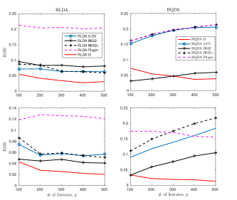
Figure 1: RMS performance of the proposed general consistent estimators (RLDA G and RQDA G) compared with the benchmark estimation techniques. We consider equal training size ($n_{0}=n_{1}$), $\gamma=1$ and $\left[\mathbf{\Sigma}_{0}\right]_{i,j}=0.6^{|i-j|}$, $\mathbf{\Sigma}_{1}=\mathbf{\Sigma}_{0}+3\mathbf{S}_{p}$, $\bm{\mu}_{0}=\left[1,\mathbf{0}_{1\times\left(p-1\right)}\right]^{T}$ and $\bm{\mu}_{1}=\bm{\mu}_{0}+\frac{0.8}{\sqrt{p}}\mathbf{1}_{p\times 1}$. The first row treats the case where $n_{0}=p/2$ whereas the second row treats the case $n_{0}=p$. The testing error is evaluated over a testing set of size $1000$ samples for both classes and averaged over $1000$ realizations.

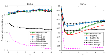
Figure 2: Average misclassification rate versus the regularization parameter $\gamma$. We consider $p=100$ features with equal training size ($n_{0}=n_{1}=p$), $\left[\mathbf{\Sigma}_{0}\right]_{i,j}=0.6^{|i-j|}$, $\mathbf{\Sigma}_{1}=\mathbf{\Sigma}_{0}+3\mathbf{S}_{p}$, $\bm{\mu}_{0}=\left[1,\mathbf{0}_{1\times\left(p-1\right)}\right]^{T}$ and $\bm{\mu}_{1}=\bm{\mu}_{0}+\frac{0.8}{\sqrt{p}}\mathbf{1}_{p\times 1}$. The testing error is evaluated over a testing set of size $1000$ samples for both classes and averaged over $1000$ realizations.

In Figure 1, we observe that the naive plugin estimator has the worst RMS performance for both classifiers in most cases. This is simply explained by the fact that when $p$ and $n_{i}$ have the same order of magnitude, the sample estimates are inaccurate which leads to a medicocre RMS performance. On another front, it is clear for both settings ($n_{i}=p/2$ and $n_{i}=p$) that the proposed G-estimator achieves a suitable RMS performance beating 5-fold cross validation and the bootstrap. In Figure 2, we examine the performance of the different error estimators against the regularization parameter. As shown in the Figure 2, R-LDA is less vulnerable to the choice of $\gamma$ as compared to R-QDA where the choice of $\gamma$ tends to have a higher influence on the performance. Also, for both classifiers, the proposed G-estimator is able to track the empirical error and thus permits to predict the optimal regularizer with high accuracy.

V Experiments with real data

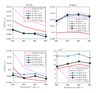
Figure 3: RMS performance of the proposed general consistent estimators (R-LDA G and R-QDA G) compared with the benchmark estimation techniques. We consider equal training size ($n_{0}=n_{1}$) and $\gamma=1$. The first row gives the performance for the USPS data with digits (5, 2) whereas the second row considers the digits (5, 6).

In this section, we examine the performance of the proposed G estimator on the public USPS dataset of handwritten digits [27]. The dataset consists of 7291 training samples of $16\times 16$ grayscale images ($p=256$ features) and 2007 testing images http://www.csie.ntu.edu.tw/~cjlin/libsvmtools/datasets/multiclass.html#usps . First, we examine the RMS performance of the different error estimators on the data for different values of the training size and for different class labels. The RMS is determined by averaging the error over a number of training sets randomly selected from the total training dataset. As shown in Figure 3, the proposed G-estimator gives a good RMS performance especially for R-QDA where it can actually outperform state-of-the art estimators such as cross validation and Bootstrap. Moreover, it is clear that the plugin estimator has a higher RMS performance for most of the considered scenarios.

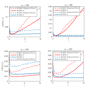
Figure 4: Average misclassification rate versus the regularization parameter $\gamma$ of the USPS dataset for different instances of digits and assuming equal training size ($n_{0}=n_{1}$). The solid red line refers to the performance of the proposed G-estimator whereas the dotted black line refers to the empirical error computed using the testing data.

Now, we turn our attention to finding the optimal $\gamma$ that results in the minimum testing error. Since the construction of the G-estimator is heavily based on the Gaussian assumption of the data, picking the regularizer that minimizes the estimated error using the G-estimator will not necessarily minimize the error computed on the testing data for USPS. One straightforward approach is to compute the testing error for all possible value of $\gamma$ in the range $\left(0,\infty\right)$, then pick the regularizer resulting in the minimum error. Obviously, this approach is far from being practical and is simply unfeasible. Motivated by this issue, we propose a two-stage optimization explained as follows.

V-A Two-stage optimization

Although real data are far from being Gaussian, the proposed G-estimator can be used to have a glimpse on the optimal regularizer. More specifically, we can use the G-estimator to determine the interval in which the optimal regularizer is likely to belong, then we perform cross validation (or testing if we have enough testing data) for multiple values of $\gamma$ inside that interval and finally pick the value that results on the minimum cross-validation error (or testing error). As seen in Figure 4, both the R-LDA and the R-QDA G-estimators are able to mimic the real behavior of the testing error when $\gamma$ varies for both situations when $n_{0}<p$ and $n_{0}>p$. Similarly to synthetic data, Figure 4 also shows how R-QDA is vulnerable to the choice of $\gamma$ which justifies the need to find a good regularization parameter $\gamma$. In Table I, we provide numerical values for the output of the two-step optimization using a confidence interval $\left(\left(\widehat{\gamma}_{G}-\frac{2}{\sqrt{p}}\right)^{+},\widehat{\gamma}_{G}+\frac{2}{\sqrt{p}}\right)$ with a uniform grid of 50 points where $\widehat{\gamma}_{G}$ is a minimizer of the G-estimator built based on the Gaussian assumption.

TABLE I: Estimates of the optimal regularizer using the two-step optimization method with their corresponding testing error.

	$\widehat{\gamma}^{R-LDA}$	$\epsilon_{testing}^{R-LDA}$	$\widehat{\gamma}^{R-QDA}$	$\epsilon_{testing}^{R-QDA}$
USPS(5, 2), $n_{0}=100$	3.54	0.0307	0.896	0.0111
USPS(5, 2), $n_{0}=400$	20.98	0.0251	1.049	0.0223
USPS(5, 6), $n_{0}=100$	4.753	0.0272	0.567	0.0272
USPS(5, 6), $n_{0}=400$	12.1572	0.01818	0.562	0.009

VI Concluding remarks

In this work, we carried out a performance analysis of the asymptotic misclassification rate for R-LDA and R-QDA based classifiers in the regime where the dimension of the training data and their number grow large with the same pace. By leveraging results from random matrix theory, we identify the growth rate regimes in which R-LDA and R-QDA result in non trivial mis-classification rates. These latter are characterized in the asymptotic regime by closed-form expressions reflecting the impact of the means and covariances of each class on the classification performance. Several insights are drawn from our results, which can guide the practitioners to choose the best classifier according to the setting into consideration. Particularly, we highlight that R-LDA achieves perfect classification rates when the difference in the mean vectors is higher than $O(p^{\alpha})$ for $\alpha>0$. The R-QDA, on the other hand, results in perfect classification when the number of significant eigenvalues of the difference between both covariance matrices scales larger than $O(\sqrt{p})$ or the difference in means is higher than $O(\sqrt{p})$. Such findings reveal a fundamental difference in the way the information about the classes means and covariances are leveraged by both methods. Unlike the R-LDA which tends to leverage only the information about the means, the R-QDA exploits both discriminative statistics, but requires a higher order in the mean difference so that it is reflected in the classification performances.

This work can be extended to study more sophisticated classifiers such as kernel Fisher discriminant analysis [28] or kernel discriminant analysis [29] where data is mapped into a feature space through a non-linear kernel prior to the application of the classifier. The extension is though not trivial since the non-linear mapping of data makes it difficult to examine the misclassification probability in closed-form.

Appendix A Proof of Theorem 1

A-A Notations

Through this appendix, the following notations are used. For $i\in\left\{0,1\right\}$, we let ${\bf X}_{i}\in\mathbb{R}^{p\times n_{i}}$ the matrix of $n_{i}$ observations associated with class $i$. Thus, there exists ${\bf Y}_{i}=\mathbf{\Sigma}_{i}^{1/2}\mathbf{Z}_{i}$ such that ${\bf X}_{i}=\bm{\Sigma}_{i}^{\frac{1}{2}}{{\bf Z}_{i}}+\bm{\mu}_{i}{\bf 1}_{n_{i}}^{T}$ where ${\bf 1}_{n_{i}}\in\mathbb{R}^{n_{i}}$ is the vector of all ones, and ${\bf Z}_{i}=\left[\mathbf{z}_{i,1},\cdots,\mathbf{z}_{i,n_{i}}\right]\in\mathbb{R}^{p\times n_{i}}$ where $\mathbf{z}_{i,j}$ are independent random vectors with standard multivariate Gaussian distribution. We define the following resolvent matrix:

$$\mathbf{Q}\left(z\right)=\left(\frac{\mathbf{Y}_{0}\mathbf{Y}_{0}^{T}}{p}+\frac{\mathbf{Y}_{1}\mathbf{Y}_{1}^{T}}{p}-z\mathbf{I}_{p}\right)^{-1}$$ (41)

the behavior of which has been extensively studied in [16, Proposition 5]. Particularly, it was shown that under assumptions 1, 2 and 3, $\mathbf{Q}\left(z\right)$ is equivalent to a deterministic matrix $\bar{\mathbf{Q}}\left(z\right)$ or $\mathbf{Q}\left(z\right)\leftrightarrow\bar{\mathbf{Q}}\left(z\right)$ in the sense that

$$\begin{split}&\frac{1}{p}\mathop{\rm tr}\mathbf{M}\left(\mathbf{Q}\left(z\right)-\bar{\mathbf{Q}}\left(z\right)\right)\to_{prob.}0.\\ &\mathbf{u}^{T}\left(\mathbf{Q}\left(z\right)-\bar{\mathbf{Q}}\left(z\right)\right)\mathbf{v}\to_{prob.}0,\end{split}$$ (42)

for all deterministic matrices $\mathbf{M}$ of bounded spectral norms and all deterministic vectors $\mathbf{u}$ and $\mathbf{v}$ of bounded euclidean norms. Moreover, it has been shown in [16, Proposition 6] that

$$\mathbf{Q}\left(z\right)\mathbf{\Sigma}_{i}\mathbf{Q}\left(z\right)\leftrightarrow\widetilde{\mathbf{Q}}_{i}\left(z\right),\;\textnormal{for}\>i\in\{0,1\}.$$ (43)

where $\widetilde{\bf Q}_{i}$ is given in (18). Based on the results of (42) and (43), we successively prove (22) and (23).

A-B Proof of (22)

With the aforementioned notations at hand, it is easy to show that $\widehat{\mathbf{\Sigma}}_{i}$ can be expressed as

$$\widehat{\mathbf{\Sigma}}_{i}=\frac{1}{n_{i}-1}\left(\mathbf{Y}_{i}\mathbf{Y}_{i}^{T}-\mathbf{Y}_{i}\frac{\mathbf{1}_{n_{i}}\mathbf{1}_{n_{i}}^{T}}{n_{i}}\mathbf{Y}_{i}^{T}\right).$$

Let $\frac{\mathbf{1}_{i}\mathbf{1}_{i}^{T}}{n_{i}}=\mathbf{O}_{i}\mathbf{E}_{i}\mathbf{O}_{i}^{T}$, be the eigenvalue decomposition of $\frac{\mathbf{1}_{i}\mathbf{1}_{i}^{T}}{n_{i}}$ where $\mathbf{E}_{i}=\mathop{\rm diag}\left(\left[1,\mathbf{0}_{(n_{i}-1)\times 1}\right]\right)$ and $\mathbf{O}_{i}$ is a $n_{i}\times n_{i}$ orthogonal matrix with first column $\frac{1}{\sqrt{n_{i}}}{\bf 1}_{n_{i}}$. Let $\tilde{\bf Y}_{i}={\bf Y}_{i}{\bf O}_{i}$. Hence

$$\begin{split}\widehat{\mathbf{\Sigma}}_{i}&=\frac{1}{n_{i}-1}\mathbf{Y}_{i}\mathbf{O}_{i}\mathbf{O}_{i}^{T}\mathbf{Y}_{i}^{T}-\frac{1}{n_{i}-1}{\mathbf{Y}_{i}\mathbf{O}_{i}}\mathbf{E}_{i}\mathbf{O}_{i}^{T}\mathbf{Y}_{i}^{T}\\ &=\frac{1}{n_{i}-1}\widetilde{\mathbf{Y}}_{i}\widetilde{\mathbf{Y}}_{i}^{T}-\frac{1}{n_{i}-1}\widetilde{\mathbf{y}}_{i,1}\widetilde{\mathbf{y}}_{i,1}^{T},\end{split}$$ (44)

where $\widetilde{\mathbf{y}}_{i,1}$ being the first column of $\widetilde{\mathbf{Y}}_{i}$. Since the Gaussian distribution is invariant to multiplication by a unitary matrix, $\tilde{\bf Y}_{i}$ has the same distribution as ${\bf Y}_{i}$. and as such matrix ${\bf H}$ can be expressed as:

$$\begin{split}\mathbf{H}&=\Biggl{[}\mathbf{I}_{p}+\frac{\gamma}{n-2}\widetilde{\mathbf{Y}}_{0}\widetilde{\mathbf{Y}}_{0}^{T}+\frac{\gamma}{n-2}\widetilde{\mathbf{Y}}_{1}\widetilde{\mathbf{Y}}_{1}^{T}-\frac{\gamma}{n-2}\widetilde{\mathbf{y}}_{0,1}\widetilde{\mathbf{y}}_{0,1}^{T}\\ &-\frac{\gamma}{n-2}\widetilde{\mathbf{y}}_{1,1}\widetilde{\mathbf{y}}_{1,1}^{T}\Biggr{]}^{-1}.\end{split}$$ (45)

Then, the following relation holds for $z=-\frac{n}{p\gamma}$

$$\mathbf{H}=-z\mathbf{Q}\left(z\right)+O_{\|.\|}(p^{-1}),$$

where $O_{\|.\|}(p^{-1})$ refers to a matrix whose spectral norm is $O(p^{-1})$. We are now ready to handle the term $G\left(\bm{\mu}_{i},\hat{\bm{\mu}}_{0},\hat{\bm{\mu}}_{1},\mathbf{H}\right)$. To start, we first express it as

$$G\left(\bm{\mu}_{i},\hat{\bm{\mu}}_{0},\hat{\bm{\mu}}_{1},\mathbf{H}\right) =\left(\frac{(-1)^{i}}{2}\bm{\mu}^{T}-\frac{1}{2n_{0}}{\bf 1}^{T}{\bf Y}_{0}-\frac{1}{2n_{1}}{\bf 1}_{n_{1}}^{T}{\bf Y}_{1}\right)$$

$$\times{\bf H}(\frac{1}{n_{0}}{\bf Y}_{0}{\bf 1}_{n_{0}}-\frac{1}{n_{1}}{\bf Y}_{1}{\bf 1}_{n_{1}}+\bm{\mu}).$$

and thus can be expanded as

$$G\left(\bm{\mu}_{i},\hat{\bm{\mu}}_{0},\hat{\bm{\mu}}_{1},\mathbf{H}\right)=\frac{\left(-1\right)^{i}}{2}\bm{\mu}^{T}\mathbf{H}\bm{\mu}+\frac{\left(-1\right)^{i}}{2n_{0}}\bm{\mu}^{T}\mathbf{H}\mathbf{Y}_{0}^{T}\mathbf{1}_{n_{0}}$$

$$+\frac{\left(-1\right)^{i+1}}{2n_{1}}\bm{\mu}^{T}\mathbf{H}\mathbf{Y}_{1}^{T}\mathbf{1}_{n_{1}}-\frac{1}{2n_{0}}\bm{\mu}^{T}\mathbf{H}\mathbf{Y}_{0}\mathbf{1}_{n_{0}}$$

$$-\frac{1}{2n_{0}^{2}}\mathbf{1}_{n_{0}}^{T}\mathbf{Y}_{0}^{T}\mathbf{HY}_{0}\mathbf{1}_{n_{0}}+\frac{1}{2n_{0}n_{1}}\mathbf{1}_{n_{0}}^{T}\mathbf{Y}_{0}^{T}\mathbf{HY}_{1}\mathbf{1}_{n_{1}}$$

$$-\frac{1}{2n_{1}}\bm{\mu}^{T}\mathbf{H}\mathbf{Y}_{1}\mathbf{1}_{n_{1}}-\frac{1}{2n_{0}n_{1}}\mathbf{1}_{n_{0}}^{T}\mathbf{Y}_{0}^{T}\mathbf{HY}_{1}\mathbf{1}_{n_{1}}$$

$$+\frac{1}{2n_{1}^{2}}\mathbf{1}_{n_{1}}^{T}\mathbf{Y}_{1}^{T}\mathbf{HY}_{1}\mathbf{1}_{n_{1}}.$$

It follows from (45) that $\tilde{\bf y}_{0,1}=\frac{1}{\sqrt{n}_{0}}{\bf Y}_{0}{\bf 1}$ and $\tilde{\bf y}_{1,1}=\frac{1}{\sqrt{n}_{1}}{\bf Y}_{1}{\bf 1}$ are independent of ${\bf H}$. The following convergence holds thus true

$$\frac{1}{n_{0}}\bm{\mu}^{T}\mathbf{H}\mathbf{Y}_{0}\mathbf{1}_{n_{0}}\to_{a.s.}0.$$

$$\frac{1}{n_{1}}\bm{\mu}^{T}\mathbf{H}\mathbf{Y}_{1}\mathbf{1}_{n_{1}}\to_{a.s.}0.$$

$$\frac{1}{n_{0}n_{1}}\mathbf{1}_{n_{0}}^{T}\mathbf{Y}_{0}^{T}\mathbf{HY}_{1}\mathbf{1}_{n_{1}}\to_{a.s.}0.$$

On the other hand, we have

$$\bm{\mu}^{T}\mathbf{H}\bm{\mu}=-z\bm{\mu}^{T}\mathbf{Q}\left(z\right)\bm{\mu}+o(1).$$ (46)

and thus from (42)

$$\bm{\mu}^{T}\mathbf{H}\bm{\mu}+z\bm{\mu}^{T}\bar{\mathbf{Q}}\left(z\right)\bm{\mu}\to_{prob.}0.$$ (47)

Moreover,

$$\frac{1}{n_{i}^{2}}\mathbf{1}_{n_{i}}^{T}\mathbf{Y}_{i}^{T}\mathbf{H}\mathbf{Y}_{i}\mathbf{1}_{n_{i}} =\frac{1}{n_{i}}\widetilde{\mathbf{y}}_{i,1}^{T}\mathbf{H}\widetilde{\mathbf{y}}_{i,1}$$

Again, from the independence of $\widetilde{\mathbf{y}}_{i}$ and $\mathbf{H}$ and the application of the trace Lemma [15, Theorem 3.7] it follows that:

$$\frac{1}{n_{i}^{2}}\mathbf{1}_{n_{i}}\mathbf{Y}_{i}^{T}\mathbf{H}\mathbf{Y}_{i}\mathbf{1}_{n_{i}}-\frac{1}{n_{i}}\mathop{\rm tr}\mathbf{\Sigma}_{i}\mathbf{H}\to_{a.s.}0.$$

which gives using (42),

$$\frac{1}{n_{i}^{2}}\mathbf{1}_{n_{i}}\mathbf{Y}_{i}^{T}\mathbf{H}\mathbf{Y}_{i}\mathbf{1}_{n_{i}}+\frac{z}{n_{i}}\mathop{\rm tr}\mathbf{\Sigma}_{i}\bar{\mathbf{Q}}\left(z\right)\to_{prob.}0.$$

This completes the proof of (22).

A-C Proof of (23)

Using the notations employed in the proof of (22), $D(\overline{\bf x}_{0},\overline{\bf x}_{1},{\bf H},\bm{\Sigma}_{i})$ can be expressed as:

$$\begin{split}D(\hat{\bm{\mu}}_{0},\hat{\bm{\mu}}_{1},{\bf H},\bm{\Sigma}_{i})&=\left(\bm{\mu}^{T}+{\bf 1}_{n_{0}}^{T}\frac{{\bf Y}_{0}}{n_{0}}-{\bf 1}_{n_{1}}^{T}\frac{{\bf Y}_{1}}{n_{1}}\right){\bf H}\bm{\Sigma}_{i}{\bf H}\\ &\times\left(\bm{\mu}+{{\bf Y}_{0}}\frac{{\bf 1}_{n_{0}}}{n_{0}}-{{\bf Y}_{1}}\frac{{\bf 1}_{n_{1}}}{n_{1}}\right).\end{split}$$ (48)

As in the proof (22), from the independence of $\frac{1}{n_{1}}{\bf Y}_{1}{\bf 1}$ and $\frac{1}{n_{0}}{\bf Y}_{0}{\bf 1}$ of ${\bf H}$, it is easy to see that the cross-products in (48) will converge to zero almost surely. We thus have:

$$D\left(\hat{\bm{\mu}}_{0},\hat{\bm{\mu}}_{1},\mathbf{H},\mathbf{\Sigma}_{i}\right) =\bm{\mu}^{T}\mathbf{H\Sigma}_{i}\mathbf{H}\bm{\mu}+\frac{1}{n_{0}^{2}}\mathbf{1}_{n_{0}}^{T}\mathbf{Y}_{0}^{T}\mathbf{H\Sigma}_{i}\mathbf{H}\mathbf{Y}_{0}\mathbf{1}_{n_{0}}$$

$$+\frac{1}{n_{1}^{2}}\mathbf{1}_{n_{1}}^{T}\mathbf{Y}_{1}^{T}\mathbf{H\Sigma}_{i}\mathbf{HY}_{1}\mathbf{1}_{n_{1}}.$$

Finally, we use (43) to obtain

$$\bm{\mu}^{T}\mathbf{H\Sigma}_{i}\mathbf{H}\bm{\mu}-z^{2}\bm{\mu}^{T}\widetilde{\mathbf{Q}}_{i}\left(z\right)\bm{\mu}\to_{prob.}0$$

$$\frac{1}{n_{j}^{2}}\mathbf{1}_{n_{j}}^{T}\mathbf{Y}_{j}^{T}\mathbf{H\Sigma}_{i}\mathbf{H}\mathbf{Y}_{j}\mathbf{1}_{n_{j}}-\frac{z^{2}}{n_{j}}\mathop{\rm tr}\mathbf{\Sigma}_{j}\widetilde{\mathbf{Q}}_{i}\left(z\right)\to_{prob.}0,\>j=1-i.$$

which completes the proof of (23).

Appendix B Proof of Proposition 1

To reduce the amount of notations, we drop the class subscript $i$. In all the proof $\mathbf{B}$ plays the role of $\mathbf{B}_{i}$ and $\mathbf{y}$ plays the role of $\mathbf{y}_{i}$, for $i\in\{0,1\}$. To begin with, let $\mathbf{B}=\mathbf{U}_{b}\mathbb{B}\mathbf{U}_{b}^{T}$ be the eigenvalue decomposition of ${\bf B}$, so that ${\bm{z}}^{T}\mathbf{\bf B}{\bm{z}}+2{\bm{z}}^{T}{\bf r}$ has the same distribution as:

$$g\left({\bf z}\right)\triangleq \sum_{j=1}^{p}{\left(\alpha_{j}z_{j}^{2}+2z_{j}\tilde{r}_{j}\right)},$$

where $\mathbf{\tilde{y}}=\mathbf{U}_{b}\mathbf{r}$, $\alpha_{i}$ diagonal elements of $\mathbb{B}$ and $z_{j}$ and $\tilde{r}_{j}$ are respectively the $j$th entries of $\bm{\omega}$ and $\mathbf{\tilde{y}}$. Let $\mathbf{\Psi}=\left[\mathbf{X}_{0},\mathbf{X}_{1}\right]$ be the observations associated with class $0$ and $1$. Then, conditioning on $\mathbf{\Psi}$, $g\left(\bm{z}\right)$ is the sum of independent but not identically distributed r.v’s. $q_{j}=\alpha_{j}z_{j}^{2}+2z_{j}\tilde{r}_{j}$. To prove the CLT, we resort to the Lyapunov CLT Theorem, [21, Theorem 27.3]. We first calculate the mean and the variance of $r_{j}$ conditioned on $\mathbf{\Psi}$

$$\mathop{\mathbb{E}}\left[q_{j}|\mathbf{\Psi}\right] =\alpha_{j}$$

$$\text{var}\left[q_{j}|\mathbf{\Psi}\right] =\sigma_{j}^{2}=2\alpha_{j}^{2}+4\tilde{r}_{j}^{2}.$$

Define the total variance $s_{p}^{2}$ as

$$s_{p}^{2}=\sum_{j=1}^{p}\sigma_{j}^{2}=2\mathop{\rm tr}\mathbf{B}^{2}+4\mathbf{\tilde{r}}^{T}\mathbf{\tilde{r}}.$$ (49)

To prove the CLT, it suffices to check the Lyapunov’s condition. Under the setting of Proposition 1,

$$\lim_{p\to\infty}\frac{1}{s_{p}^{4}}\sum_{j=1}^{p}\mathop{\mathbb{E}}\left[\left|q_{j}-\alpha_{j}\right|^{4}||\bm{\Psi}\right]$$

$$=\lim_{p\to\infty}\frac{\sum_{j=1}^{p}60\alpha_{j}^{4}+240\alpha_{j}^{2}\tilde{r}_{j}^{2}+48\tilde{r}_{j}^{4}}{\left(2\mathop{\rm tr}\mathbf{B}^{2}+4\mathbf{\tilde{r}}^{T}\mathbf{\tilde{r}}\right)^{2}}$$

$$\leq\lim_{p\to\infty}\frac{60/p^{2}\mathop{\rm tr}{\bf B}^{2}+240/p^{2}\mathop{\rm tr}{\bf B}^{2}\|\tilde{\bf r}\|_{2}^{2}+48/p^{2}\|\tilde{\bf r}\|_{2}^{4}}{\left(2/p\mathop{\rm tr}{\bf B}^{2}+4/p\|\tilde{\bf r}\|_{2}^{2}\right)^{2}}.$$

Appendix C Proof of Theorem 2

The proof consists in showing the following convergences

$$\frac{1}{\sqrt{p}}\xi_{i}-\overline{\xi}_{i}\to_{prob.}0.$$ (50)

$$\frac{1}{\sqrt{p}}\mathop{\rm tr}\mathbf{B}_{i}-\overline{b_{i}}\to_{a.s.}0.$$ (51)

$$\frac{1}{p}\mathop{\rm tr}\mathbf{B}_{i}^{2}-\overline{B_{i}}\to_{a.s.}0.$$ (52)

$$\frac{1}{p}\mathbf{r}_{i}^{T}\mathbf{r}_{i}\to_{a.s.}0.$$ (53)

and establishing that the condition in 1 holds with probability $1$. We will prove sequentially equations (50)-(53).

C-A Proof of (50)

Using the simplified expression of $\widehat{\mathbf{\Sigma}}_{i}$ in (44), we can write

$$\mathbf{H}_{i}=\left(\mathbf{I}_{p}+\frac{\gamma}{n_{i}-1}\mathbf{Y}_{i}\mathbf{Y}_{i}^{T}-\frac{\gamma}{n_{i}-1}\mathbf{y}_{i}\mathbf{y}_{i}^{T}\right)^{-1}.$$

Recall that $\frac{1}{\sqrt{p}}\xi_{i}$ writes as

$$\frac{1}{\sqrt{p}}\xi_{i} =-\frac{1}{\sqrt{p}}\log\frac{|{\bf H}_{0}|}{|{\bf H}_{1}|}+\frac{1}{\sqrt{p}}(\bm{\mu}_{i}-\hat{\bm{\mu}}_{0})^{T}{\bf H}_{0}(\bm{\mu}_{i}-\hat{\bm{\mu}}_{0})$$

$$-\frac{1}{\sqrt{p}}(\bm{\mu}_{i}-\hat{\bm{\mu}}_{1})^{T}{\bf H}_{1}(\bm{\mu}_{i}-\hat{\bm{\mu}}_{1})+\frac{2}{\sqrt{p}}\log\frac{\pi_{1}}{\pi_{0}}.$$

Under Assumption 7, Matrix $\mathbf{H}_{i}$ follows the model in [14]. According to [14, Theorem 1],

$$\frac{1}{p}\log|\mathbf{H}_{i}|-\frac{1}{p}\left(\log|\mathbf{T}_{i}|-n_{i}\log\left(1+\gamma\delta_{i}\right)+\gamma\frac{n_{i}\delta_{i}}{1+\gamma\delta_{i}}\right)\to_{a.s.}0.$$ (54)

The convergence holds with rate $O(p^{-1})$ hence,

$$\frac{1}{\sqrt{p}}\log|\mathbf{H}_{i}|-\frac{1}{\sqrt{p}}\left(\log|\mathbf{T}_{i}|-n_{i}\log\left(1+\gamma\delta_{i}\right)+\gamma\frac{n_{i}\delta_{i}}{1+\gamma\delta_{i}}\right)\to_{prob.}0.$$

and

$$\frac{1}{\sqrt{p}}\left(\left(\bm{\mu}_{i}-\hat{\bm{\mu}}_{0}\right)^{T}\mathbf{H}_{0}\left(\bm{\mu}_{i}-\hat{\bm{\mu}}_{0}\right)-\left(\bm{\mu}_{i}-\hat{\bm{\mu}}_{1}\right)^{T}\mathbf{H}_{1}\left(\bm{\mu}_{i}-\hat{\bm{\mu}}_{1}\right)\right)$$

$$-\frac{\left(-1\right)^{i+1}}{\sqrt{p}}\bm{\mu}^{T}\mathbf{T}_{1-i}\bm{\mu}\to_{prob.}0.$$

C-B Proof of (51)

From [14], we know that

$$\frac{1}{p}\mathop{\rm tr}\mathbf{\Sigma}_{i}\mathbf{H}_{i}-\frac{1}{p}\mathop{\rm tr}\mathbf{\Sigma}_{i}\mathbf{T}_{i}\to_{a.s.}0$$ (55)

where the above convergence holds with rate $O(p^{-1})$.

Thus,

$$\frac{1}{\sqrt{p}}\mathop{\rm tr}\mathbf{B}_{i}-\frac{1}{\sqrt{p}}\mathop{\rm tr}\mathbf{\Sigma}_{i}\left(\mathbf{T}_{1}-\mathbf{T}_{0}\right)\to_{prob.}0.$$

C-C Proof of (52)

To prove (52), we need the following lemma, the proof of which is omitted since it follows from the techniques established in [14]

Lemma. 1.

Let ${\bf A}$ be a matrix with uniformly bounded spectral norm. Then, for $i\in\{0,1\}$ the following convergence holds true

$$\begin{split}&\frac{1}{p}\mathop{\rm tr}\mathbf{A}\mathbf{H}_{i}\mathbf{A}\mathbf{H}_{i}-\left[\frac{1}{p}\mathop{\rm tr}\mathbf{T}_{i}^{2}\mathbf{A}^{2}+\frac{\gamma^{2}\tilde{\phi}_{i}}{1-\gamma^{2}\phi_{i}\tilde{\phi}_{i}}\left(\frac{1}{n_{i}}\mathop{\rm tr}\mathbf{A}\mathbf{\Sigma}_{i}\mathbf{T}_{i}^{2}\right)^{2}\right]\\ &\to_{a.s.}0.\end{split}$$ (56)

With the above Lemma at hand, we are now ready to handle $\frac{1}{p}\mathop{\rm tr}\mathbf{B}_{i}^{2}$.

$$\frac{1}{p}\mathop{\rm tr}\mathbf{B}_{i}^{2} =\frac{1}{p}\mathop{\rm tr}\mathbf{\Sigma}_{i}\left(\mathbf{H}_{1}-\mathbf{H}_{0}\right)\mathbf{\Sigma}_{i}\left(\mathbf{H}_{1}-\mathbf{H}_{0}\right)$$

$$=\frac{1}{p}\mathop{\rm tr}\mathbf{\Sigma}_{i}\mathbf{H}_{1}\mathbf{\Sigma}_{i}\mathbf{H}_{1}+\frac{1}{p}\mathop{\rm tr}\mathbf{\Sigma}_{i}\mathbf{H}_{0}\mathbf{\Sigma}_{i}\mathbf{H}_{0}-\frac{2}{p}\mathop{\rm tr}\mathbf{\Sigma}_{i}\mathbf{H}_{0}\mathbf{\Sigma}_{i}\mathbf{H}_{1}.$$

By product of Lemma 1, we can easily get

$$\frac{1}{p}\mathop{\rm tr}\mathbf{\Sigma}_{i}\mathbf{H}_{i}\mathbf{\Sigma}_{i}\mathbf{H}_{i}-\frac{c\phi_{i}}{1-\gamma^{2}\phi_{i}\tilde{\phi}_{i}}\to_{a.s.}0$$ (57)

$$\begin{split}&\frac{1}{p}\mathop{\rm tr}\mathbf{\Sigma}_{i}\mathbf{H}_{1-i}\mathbf{\Sigma}_{i}\mathbf{H}_{1-i}\\ &-\left[\frac{1}{p}\mathop{\rm tr}\mathbf{\Sigma}_{i}^{2}\mathbf{T}_{1-i}^{2}+\frac{\gamma^{2}c\tilde{\phi}_{1-i}\left(\frac{1}{n_{i}}\mathop{\rm tr}\mathbf{\Sigma}_{i}\mathbf{\Sigma}_{1-i}\mathbf{T}_{1-i}^{2}\right)^{2}}{1-\gamma^{2}\phi_{1-i}\tilde{\phi}_{1-i}}\right]\\ &\to_{a.s.}0.\end{split}$$ (58)

Finally, it is straightforward to obtain

$$\frac{1}{p}\mathop{\rm tr}\mathbf{\Sigma}_{i}\mathbf{H}_{1}\mathbf{\Sigma}_{i}\mathbf{H}_{0}-\frac{1}{p}\mathop{\rm tr}\mathbf{\Sigma}_{i}\mathbf{T}_{1}\mathbf{\Sigma}_{i}\mathbf{T}_{0}\to_{a.s.}0.$$ (59)

This completes the proof of (52).

C-D Proof of (53)

Let $i\in\left\{0,1\right\}$. Then, one can see that:

$$\frac{1}{p}\mathbf{r}_{i}^{T}\mathbf{r}_{i}-\frac{1}{p}\bm{\mu}^{T}\mathbf{H}_{1-i}\mathbf{\Sigma}_{i}\mathbf{H}_{1-i}\bm{\mu}\to_{prob.}0,$$ (60)

where by Assumptions 6 and 7

$$\frac{1}{p}\bm{\mu}^{T}\mathbf{H}_{1-i}\mathbf{\Sigma}_{i}\mathbf{H}_{1-i}\bm{\mu}=O\left(\frac{1}{\sqrt{p}}\right).$$

Finally, by applying the continous mapping theorem [30], we complete the proof of Theorem 2.

Now, to conclude we need to check that the condition in Proposition 1 holds with probability 1. This can be easily seen by replacing in (27), $\frac{1}{p}\mathop{\rm tr}{\bf B}^{2}$ by its deterministic equivalent and noting that it has order $O(1)$.

Appendix D Proof of Proposition 2

To prove Proposition 2, it suffices to show

$$\frac{1}{\sqrt{p}}\left(\frac{n_{0}\delta_{0}}{1+\gamma\delta_{0}}-\frac{n_{1}\delta_{1}}{1+\gamma\delta_{1}}\right)=O\left(1\right)$$ (61)

$$\frac{1}{\sqrt{p}}\left(n_{1}\log\left(1+\gamma\delta_{1}\right)-n_{0}\log\left(1+\gamma\delta_{0}\right)\right)=O\left(1\right)$$ (62)

$$\frac{1}{\sqrt{p}}\left(\log|\mathbf{T}_{0}|-\log|\mathbf{T}_{1}|\right)=O\left(1\right)$$ (63)

Relying on Assumption 5, we can assume $n_{0}=n_{1}=\frac{n}{2}$. To begin, we first note that

$$\frac{\delta_{0}}{1+\gamma\delta_{0}}-\frac{\delta_{1}}{1+\gamma\delta_{1}}=\frac{1}{\left(1+\gamma\delta_{0}\right)\left(1+\gamma\delta_{1}\right)}\left(\delta_{0}-\delta_{1}\right).$$

On the other hand,

$$\delta_{0}-\delta_{1} =\frac{2}{n}\mathop{\rm tr}\mathbf{\Sigma}_{0}\mathbf{T}_{0}-\frac{2}{n}\mathop{\rm tr}\mathbf{\Sigma}_{1}\mathbf{T}_{1}$$

$$=\frac{2}{n}\mathop{\rm tr}\mathbf{\Sigma}_{0}\left(\mathbf{T}_{0}-\mathbf{T}_{1}\right)+\frac{2}{n}\mathop{\rm tr}\left(\mathbf{\Sigma}_{0}-\mathbf{\Sigma}_{1}\right)\mathbf{T}_{1}.$$

Recall that for invertible square matrices $\mathbf{A}$ and $\mathbf{B}$, we have the resolvent identity given by

$$\mathbf{A}^{-1}-\mathbf{B}^{-1}=\mathbf{A}^{-1}\left(\mathbf{B}-\mathbf{A}\right)\mathbf{B}^{-1}.$$ (64)

Thus,

$$\delta_{0}-\delta_{1}$$

$$=\frac{2}{n}\mathop{\rm tr}\mathbf{\Sigma}_{0}\mathbf{T}_{0}\left(\mathbf{T}_{1}^{-1}-\mathbf{T}_{0}^{-1}\right)\mathbf{T}_{1}+\frac{2}{n}\mathop{\rm tr}\left(\mathbf{\Sigma}_{0}-\mathbf{\Sigma}_{1}\right)\mathbf{T}_{1}$$

$$=\frac{2}{n}\mathop{\rm tr}\mathbf{\Sigma}_{0}\mathbf{T}_{0}\left(\frac{\gamma}{1+\gamma\delta_{1}}\mathbf{\Sigma}_{1}-\frac{\gamma}{1+\gamma\delta_{0}}\mathbf{\Sigma}_{0}\right)\mathbf{T}_{1}+\frac{2}{n}\mathop{\rm tr}\left(\mathbf{\Sigma}_{0}-\mathbf{\Sigma}_{1}\right)\mathbf{T}_{1}$$

$$=\frac{2\gamma}{n}\mathop{\rm tr}\mathbf{\Sigma}_{0}\mathbf{T}_{0}\left(\frac{\mathbf{\Sigma}_{1}}{1+\gamma\delta_{1}}-\frac{\mathbf{\Sigma}_{1}}{1+\gamma\delta_{0}}+\frac{\mathbf{\Sigma}_{1}}{1+\gamma\delta_{0}}-\frac{\mathbf{\Sigma}_{0}}{1+\gamma\delta_{0}}\right)\mathbf{T}_{1}$$

$$+\frac{2}{n}\mathop{\rm tr}\left(\mathbf{\Sigma}_{0}-\mathbf{\Sigma}_{1}\right)\mathbf{T}_{1}$$

$$=\frac{\gamma^{2}\left(\delta_{0}-\delta_{1}\right)}{\left(1+\gamma\delta_{0}\right)\left(1+\gamma\delta_{1}\right)}\frac{2}{n}\mathop{\rm tr}\mathbf{\Sigma}_{0}\mathbf{T}_{0}\mathbf{\Sigma}_{1}\mathbf{T}_{1}$$

$$-\frac{\gamma}{1+\gamma\delta_{0}}\frac{2}{n}\mathop{\rm tr}\mathbf{\Sigma}_{0}\mathbf{T}_{0}\left(\mathbf{\Sigma}_{0}-\mathbf{\Sigma}_{1}\right)\mathbf{T}_{1}+\frac{2}{n}\mathop{\rm tr}\left(\mathbf{\Sigma}_{0}-\mathbf{\Sigma}_{1}\right)\mathbf{T}_{1}.$$

Therefore,

$$\left(\delta_{0}-\delta_{1}\right)\left[1-\frac{2\gamma^{2}}{\left(1+\gamma\delta_{0}\right)\left(1+\gamma\delta_{1}\right)}\frac{1}{n}\mathop{\rm tr}\mathbf{\Sigma}_{0}\mathbf{T}_{0}\mathbf{\Sigma}_{1}\mathbf{T}_{1}\right]$$

$$=-\frac{\gamma}{1+\gamma\delta_{0}}\frac{2}{n}\mathop{\rm tr}\mathbf{\Sigma}_{0}\mathbf{T}_{0}\left(\mathbf{\Sigma}_{0}-\mathbf{\Sigma}_{1}\right)\mathbf{T}_{1}+\frac{2}{n}\mathop{\rm tr}\left(\mathbf{\Sigma}_{0}-\mathbf{\Sigma}_{1}\right)\mathbf{T}_{1}.$$

or equivalently

$$\delta_{0}-\delta_{1} =\left[1-\frac{2\gamma^{2}}{\left(1+\gamma\delta_{0}\right)\left(1+\gamma\delta_{1}\right)}\frac{1}{n}\mathop{\rm tr}\mathbf{\Sigma}_{0}\mathbf{T}_{0}\mathbf{\Sigma}_{1}\mathbf{T}_{1}\right]^{-1}$$

$$\times\left[-\frac{2\gamma}{1+\gamma\delta_{0}}\frac{1}{n}\mathop{\rm tr}\mathbf{\Sigma}_{0}\mathbf{T}_{0}\left(\mathbf{\Sigma}_{0}-\mathbf{\Sigma}_{1}\right)\mathbf{T}_{1}+\frac{2}{n}\mathop{\rm tr}\left(\mathbf{\Sigma}_{0}-\mathbf{\Sigma}_{1}\right)\mathbf{T}_{1}\right].$$

All in all, we have

$$\begin{split}&\frac{\delta_{0}}{1+\gamma\delta_{0}}-\frac{\delta_{1}}{1+\gamma\delta_{1}}\\ &=\frac{1}{\left(1+\gamma\delta_{0}\right)\left(1+\gamma\delta_{1}\right)}\left[1-\frac{2\gamma^{2}}{\left(1+\gamma\delta_{0}\right)\left(1+\gamma\delta_{1}\right)}\frac{1}{n}\mathop{\rm tr}\mathbf{\Sigma}_{0}\mathbf{T}_{0}\mathbf{\Sigma}_{1}\mathbf{T}_{1}\right]^{-1}\\ &\times\left[-\frac{\gamma}{1+\gamma\delta_{0}}\frac{2}{n}\mathop{\rm tr}\mathbf{\Sigma}_{0}\mathbf{T}_{0}\left(\mathbf{\Sigma}_{0}-\mathbf{\Sigma}_{1}\right)\mathbf{T}_{1}+\frac{1}{n}\mathop{\rm tr}\left(\mathbf{\Sigma}_{0}-\mathbf{\Sigma}_{1}\right)\mathbf{T}_{1}\right]\end{split}$$ (65)

To guarantee that the left hand side of (65) does not blow up, we shall prove that

$$\lim\inf_{p}\left(1-\frac{2\gamma^{2}}{\left(1+\gamma\delta_{0}\right)\left(1+\gamma\delta_{1}\right)}\frac{1}{n}\mathop{\rm tr}\mathbf{\Sigma}_{0}\mathbf{T}_{0}\mathbf{\Sigma}_{1}\mathbf{T}_{1}\right)>0.$$ (66)

or equivalently

$$\lim\sup_{p}\frac{2\gamma^{2}}{\left(1+\gamma\delta_{0}\right)\left(1+\gamma\delta_{1}\right)}\frac{1}{n}\mathop{\rm tr}\mathbf{\Sigma}_{0}\mathbf{T}_{0}\mathbf{\Sigma}_{1}\mathbf{T}_{1}<1.$$ (67)

For that, recall that for a symmetric matrix $\mathbf{A}$ and non-negative definite matrix $\mathbf{B}$ [31], we have

$$\mathop{\rm tr}\mathbf{AB}\leq\|\mathbf{A}\|\mathop{\rm tr}\mathbf{B}.$$ (68)

Thus,

$$\frac{\gamma^{2}}{\left(1+\gamma\delta_{0}\right)\left(1+\gamma\delta_{1}\right)}\frac{1}{n}\mathop{\rm tr}\mathbf{\Sigma}_{0}\mathbf{T}_{0}\mathbf{\Sigma}_{1}\mathbf{T}_{1}$$

$$\leq\frac{\gamma^{2}\|\mathbf{\Sigma}_{0}\mathbf{T}_{0}\|}{\left(1+\gamma\delta_{0}\right)\left(1+\gamma\delta_{1}\right)}\underbrace{\frac{1}{n}\mathop{\rm tr}\mathbf{\Sigma}_{1}\mathbf{T}_{1}}_{\delta_{1}/2}=\underbrace{\frac{\gamma\delta_{1}/2}{1+\gamma\delta_{1}}}_{<1/2}\frac{\gamma\|\mathbf{\Sigma}_{0}\mathbf{T}_{0}\|}{1+\gamma\delta_{0}}$$

$$<\frac{\gamma/2\|\mathbf{\Sigma}_{0}\mathbf{T}_{0}\|}{1+\gamma\delta_{0}}.$$

Since $\mathbf{\Sigma}_{0}$ and $\mathbf{T}_{0}$ share the same eigenvectors, there exists a $\lambda$ an eigenvalue of $\mathbf{\Sigma}_{0}$ such that

$$\|\mathbf{\Sigma}_{0}\mathbf{T}_{0}\|=\frac{\lambda}{1+\frac{\gamma\lambda}{1+\gamma\delta_{0}}}.$$

Thus,

$$\frac{2\gamma^{2}}{\left(1+\gamma\delta_{0}\right)\left(1+\gamma\delta_{1}\right)}\frac{1}{n}\mathop{\rm tr}\mathbf{\Sigma}_{0}\mathbf{T}_{0}\mathbf{\Sigma}_{1}\mathbf{T}_{1}<\frac{\gamma\|\mathbf{\Sigma}_{0}\mathbf{T}_{0}\|}{1+\gamma\delta_{0}}$$

$$=\frac{\frac{\gamma\lambda}{1+\frac{\gamma\lambda}{1+\gamma\delta_{0}}}}{1+\gamma\delta_{0}}=\frac{\frac{\gamma\lambda}{1+\gamma\delta_{0}}}{1+\frac{\gamma\lambda}{1+\gamma\delta_{0}}}<1.$$

Thus, (67) holds. Using Assumptions 5 and 7 and by (67)

$$\frac{1}{\left(1+\gamma\delta_{0}\right)\left(1+\gamma\delta_{1}\right)}$$

$$\times\left(1-\frac{2\gamma^{2}}{\left(1+\gamma\delta_{0}\right)\left(1+\gamma\delta_{1}\right)}\frac{1}{n}\mathop{\rm tr}\mathbf{\Sigma}_{0}\mathbf{T}_{0}\mathbf{\Sigma}_{1}\mathbf{T}_{1}\right)^{-1}=O\left(1\right),$$

which implies using Assumption 8 that

$$\delta_{0}-\delta_{1}=O\left(\frac{1}{\sqrt{p}}\right).$$ (69)

This gives the claim of (61). For (62), and using the inequality $\log\left(x\right)\leq x-1$, for $x>0$ we can show that

$$\begin{vmatrix}\log\left(1+\gamma\delta_{1}\right)-\log\left(1+\gamma\delta_{0}\right)\end{vmatrix}=\begin{vmatrix}\log\frac{1+\gamma\delta_{1}}{1+\gamma\delta_{0}}\end{vmatrix}$$

$$=\begin{vmatrix}\log\left(1+\gamma\frac{\delta_{1}-\delta_{0}}{1+\gamma\delta_{0}}\right)\end{vmatrix}\leq\frac{\gamma\begin{vmatrix}\delta_{0}-\delta_{1}\end{vmatrix}}{1+\gamma\min\left(\delta_{0},\delta_{1}\right)}.$$

Following the result of (61), (62) also holds.
As for (63), it suffices to notice that:

$$\frac{1}{\sqrt{p}}\log\det{\bf T}_{0}{\bf T}_{1}^{-1}$$

$$=\frac{1}{\sqrt{p}}\log\det\left({\bf I}_{p}+{\bf T}_{0}^{\frac{1}{2}}\left(\gamma\tilde{\delta_{1}}\bm{\Sigma}_{1}-\gamma\tilde{\delta_{0}}\bm{\Sigma}_{0}\right){\bf T}_{0}^{\frac{1}{2}}\right)$$

$$=\frac{1}{\sqrt{p}}\log\det\left[{\bf I}_{p}+\gamma\tilde{\delta}_{1}{\bf T}_{0}(\bm{\Sigma}_{1}-\bm{\Sigma}_{0})+\frac{\tilde{\delta}_{1}-\tilde{\delta}_{0}}{\tilde{\delta}_{0}}\left(\mathbf{I}_{p}-\mathbf{T}_{0}\right)\right]$$

Define $\mathbf{\Phi}$ the matrix that has the same eigenvectors as $\mathbf{\Sigma}_{1}-\mathbf{\Sigma}_{0}$ with eigenvalues $\phi_{i}=|\lambda_{i}\left(\mathbf{\Sigma}_{1}-\mathbf{\Sigma}_{0}\right)|$, $i=1,\cdots,p$. Then, since ${\bf T}_{0}\preceq{\bf I}_{p}$, we have the following

$$\left|\frac{1}{\sqrt{p}}\log\det{\bf T}_{0}{\bf T}_{1}^{-1}\right|$$

$$\leq\frac{1}{\sqrt{p}}\log\det\left[\mathbf{I}_{p}+\gamma\tilde{\delta}_{1}{\bf T}_{0}^{\frac{1}{2}}\mathbf{\Phi}{\bf T}_{0}^{\frac{1}{2}}+\frac{\left|\tilde{\delta}_{1}-\tilde{\delta}_{0}\right|}{\tilde{\delta}_{0}}\mathbf{I}_{p}\right].$$

Given that $0\preceq\mathbf{\Phi}$, we have

$$\frac{1}{\sqrt{p}}\log\det\left[\mathbf{I}_{p}+\gamma\tilde{\delta}_{1}{\bf T}_{0}^{\frac{1}{2}}\mathbf{\Phi}{\bf T}_{0}^{\frac{1}{2}}+\frac{\left|\tilde{\delta}_{1}-\tilde{\delta}_{0}\right|}{\tilde{\delta}_{0}}\mathbf{I}_{p}\right]$$

$$\leq\frac{1}{\sqrt{p}}\mathop{\rm tr}\left[\gamma\tilde{\delta}_{1}\mathbf{\Phi}{\bf T}_{0}+\frac{\left|\tilde{\delta}_{1}-\tilde{\delta}_{0}\right|}{\tilde{\delta}_{0}}\mathbf{I}_{p}\right]$$

By Assumption 8, $\frac{1}{\sqrt{p}}\mathop{\rm tr}\left[\gamma\tilde{\delta}_{1}\mathbf{\Phi}{\bf T}_{0}+\frac{\left|\tilde{\delta}_{1}-\tilde{\delta}_{0}\right|}{\tilde{\delta}_{0}}\mathbf{I}_{p}\right]=O\left(1\right)$. This completes the proof.

Appendix E Proof of Theorem 3

We start the proof by showing the following

$$G\left(\hat{\bm{\mu}}_{i},\hat{\bm{\mu}}_{0},\hat{{\bm{\mu}}}_{1},\mathbf{H}\right)+\left(-1\right)^{i+1}\widehat{\theta}_{i}-G\left(\bm{\mu}_{i},{\hat{\bm{\mu}}}_{0},\hat{\bm{\mu}}_{1},\mathbf{H}\right)\to_{a.s.}0.$$

To this end, note that

$$G\left(\hat{\bm{\mu}}_{i},\hat{\bm{\mu}}_{0},\hat{\bm{\mu}}_{1},\mathbf{H}\right)=G\left(\bm{\mu}_{i},\hat{\bm{\mu}}_{0},\hat{\bm{\mu}}_{1},\mathbf{H}\right)+\frac{\mathbf{1}_{n_{i}}^{T}}{n_{i}}\mathbf{Y}_{i}\mathbf{H}\left(\hat{\bm{\mu}}_{0}-\hat{\bm{\mu}}_{1}\right).$$

Using the same arguments used to prove (22), we can easily show that

$$G\left(\hat{\bm{\mu}}_{i},\hat{\bm{\mu}}_{0},\hat{\bm{\mu}}_{1},\mathbf{H}\right)=G\left(\bm{\mu}_{i},\hat{\bm{\mu}}_{0},\hat{\bm{\mu}}_{1},\mathbf{H}\right)+\frac{\left(-1\right)^{i}}{n_{i}}\mathop{\rm tr}\mathbf{\Sigma}_{i}\mathbf{H}+o(1)$$

It remains now to show that

$$\widehat{\theta}_{i}-\frac{1}{n_{i}}\mathop{\rm tr}\mathbf{\Sigma}_{i}\mathbf{H}\to_{a.s.}0.$$ (70)

To this end, we examine the convergence of the quantity $\frac{1}{n_{i}}\mathop{\rm tr}\widehat{\mathbf{\Sigma}}_{i}\mathbf{H}$. Recall from (44) that

$$\widehat{\mathbf{\Sigma}}_{i} =\frac{1}{n_{i}-1}\widetilde{\mathbf{Y}}_{i}\widetilde{\mathbf{Y}}_{i}^{T}-\frac{1}{n_{i}-1}\widetilde{\mathbf{y}}_{i,1}\widetilde{\mathbf{y}}_{i,1}^{T}$$

$$=\frac{1}{n_{i}-1}\sum_{j=1}^{n_{i}}\widetilde{\mathbf{y}}_{i,j}\widetilde{\mathbf{y}}_{i,j}^{T}-\frac{1}{n_{i}-1}\widetilde{\mathbf{y}}_{i,1}\widetilde{\mathbf{y}}_{i,1}^{T}$$

Let ${\bf H}_{[j]}=\left(\gamma\widehat{\bm{\Sigma}}-\frac{\gamma}{n-2}\widetilde{\bf y}_{i,j}\widetilde{\bf y}_{i,j}^{T}+{\bf I}_{p}\right)^{-1}$ Thus,

$$\frac{1}{n_{i}}\mathop{\rm tr}\widehat{\mathbf{\Sigma}}_{i}\mathbf{H}=\frac{1}{n_{i}}\sum_{j=2}^{n_{i}}\frac{\frac{1}{n_{i}-1}\widetilde{\bf y}_{i,j}^{T}{\bf H}_{[j]}\widetilde{\bf y}_{i,j}}{1+\frac{\gamma}{n-2}\widetilde{\bf y}_{i,j}^{T}{\bf H}_{[j]}\widetilde{\bf y}_{i,j}}$$

Thanks to the independence between $\mathbf{H}_{j}$ and $\widetilde{\mathbf{y}}_{i,j}$ and by simple application of the trace Lemma [15], we have

$$\frac{1}{n_{i}}\mathop{\rm tr}\widehat{\mathbf{\Sigma}}_{i}\mathbf{H}-\frac{1}{n_{i}}\mathop{\rm tr}\mathbf{\Sigma}_{i}\mathbf{H}\frac{1}{1+\frac{\gamma}{n-2}\mathop{\rm tr}\bm{\Sigma}_{i}{\bf H}}\to_{a.s.}0.$$

By simple manipulations, we have the convergence in (70).

Now, using the same tricks consisting in using the inversion Lemma along with the trace Lemma, we obtain

$$\widehat{\psi}_{i}^{2}D\left({\hat{\bm{\mu}}}_{0},\hat{\bm{\mu}}_{1},\mathbf{H},\widehat{\mathbf{\Sigma}}_{i}\right)-D\left({\hat{\bm{\mu}}}_{0},\hat{\bm{\mu}}_{1},\mathbf{H},\mathbf{\Sigma}_{i}\right)\to_{a.s.}0.$$

Appendix F Proof of Theorem 4

The proof consists in proving the following convergences

$$\widehat{\xi}_{i}-\frac{1}{\sqrt{p}}\xi_{i}\to_{prob.}0.$$ (71)

$$\widehat{b}_{i}-\frac{1}{\sqrt{p}}\mathop{\rm tr}\mathbf{B}_{i}\to_{prob.}0.$$ (72)

$$\widehat{B}_{i}-\frac{1}{p}\mathop{\rm tr}\mathbf{B}_{i}^{2}\to_{prob.}0.$$ (73)

The proof of (71) is straightforward and relies on the following facts

$$\frac{1}{\sqrt{p}}\left(\bm{\mu}_{i}-\hat{\bm{\mu}}_{i}\right)^{T}\mathbf{H}_{i}\left(\bm{\mu}_{i}-\hat{\bm{\mu}}_{i}\right)\to_{prob.}0.$$

$$\frac{1}{\sqrt{p}}\left(\bar{\hat{\bm{\mu}}}_{0}-\hat{\bm{\mu}}_{1}\right)^{T}\mathbf{H}_{1-i}\left(\hat{\bm{\mu}}_{0}-\hat{\bm{\mu}}_{1}\right)$$

$$-\frac{1}{\sqrt{p}}\left(\bm{\mu}_{i}-\hat{\bm{\mu}}_{1-i}\right)^{T}\mathbf{H}_{1-i}\left(\bm{\mu}_{i}-\hat{\bm{\mu}}_{1-i}\right)\to_{prob.}0.$$

The proof of (72) relies on the fact that $\widehat{\delta}_{i}$ is a consistent estimator of $\delta_{i}$ as shown in [8], the variance of which can be shown to be of order $O(p^{-2})$. Thus,

$$\frac{1}{\sqrt{p}}\mathop{\rm tr}\mathbf{\Sigma}_{i}\mathbf{T}_{i}-\frac{n_{i}}{\sqrt{p}}\widehat{\delta}_{i}\to_{prob.}0.$$

Also, we have, for $i\in\left\{0,1\right\}$,

$$\frac{1}{\sqrt{p}}\mathop{\rm tr}\widehat{\mathbf{\Sigma}}_{i}\mathbf{H}_{1-i}-\frac{1}{\sqrt{p}}\mathop{\rm tr}\mathbf{\Sigma}_{i}\mathbf{H}_{1-i}\to_{prob.}0.$$

which gives the convergence in (72).

F-A Proof of (73)

The proof of (73) is a bit more involved than those of (71) and (72) as we will show in the following. The proof mainly relies on the application of the inversion lemma followed by the trace lemma [15]. Recall that

$$\frac{1}{p}\mathop{\rm tr}\mathbf{B}_{i}^{2} =\frac{1}{p}\mathop{\rm tr}\bm{\Sigma}_{i}{\bf H}_{1}\bm{\Sigma}_{i}{\bf H}_{1}-\frac{2}{p}\mathop{\rm tr}\bm{\Sigma}_{i}{\bf H}_{0}\bm{\Sigma}_{i}{\bf H}_{1}$$

$$+\frac{1}{p}\mathop{\rm tr}\bm{\Sigma}_{i}{\bf H}_{0}\bm{\Sigma}_{i}{\bf H}_{0}.$$

Without loss of generality, we can assume $i=1$, the other case follows naturally. We start by handling the term $\frac{1}{p}\mathop{\rm tr}\bm{\Sigma}_{1}{\bf H}_{1}\bm{\Sigma}_{1}{\bf H}_{1}$. The common method here is to replace $\mathbf{\Sigma}_{1}$ by its sample estimate $\widehat{\mathbf{\Sigma}}_{1}$, then compute the limit of the obtained expression and perform the necessary corrections to obtain the estimate of interest. In fact, we have

$$\frac{1}{p}\mathop{\rm tr}\widehat{\bm{\Sigma}}_{1}{\bf H}_{1}\widehat{\bm{\Sigma}}_{1}{\bf H}_{1}=\frac{1}{p}\sum_{j=1}^{n_{1}-1}\sum_{k=1}^{n_{1}-1}\frac{1}{p}\mathop{\rm tr}\frac{\widetilde{\bf y}_{1,j}\widetilde{\bf y}_{1,j}^{T}}{n_{1}-1}{\bf H}_{1}\frac{\widetilde{\bf y}_{1,k}\widetilde{\bf y}_{1,k}^{T}}{n_{1}-1}{\bf H}_{1}$$

$$=\frac{1}{p}\sum_{j=1}^{n_{1}-1}\sum_{k\neq j}\mathop{\rm tr}\frac{\widetilde{\bf y}_{1,j}\widetilde{\bf y}_{1,j}^{T}}{n_{1}-1}{\bf H}_{1}\frac{\widetilde{\bf y}_{1,k}\widetilde{\bf y}_{1,k}^{T}}{n_{1}-1}{\bf H}_{1}$$

$$+\frac{1}{p}\sum_{j=1}^{n_{1}-1}\mathop{\rm tr}\frac{\widetilde{\bf y}_{1,j}\widetilde{\bf y}_{1,j}^{T}}{n_{1}-1}{\bf H}_{1}\frac{\widetilde{\bf y}_{1,j}\widetilde{\bf y}_{1,j}^{T}}{n_{1}-1}{\bf H}_{1}$$

Using the inversion lemma, we handle the first term in the previous equation as follows

$$\frac{1}{p}\sum_{j=2}^{n_{1}-1}\sum_{k\neq j}\mathop{\rm tr}\frac{\widetilde{\bf y}_{1,j}\widetilde{\bf y}_{1,j}^{T}}{n_{1}-1}{\bf H}_{1}\frac{\widetilde{\bf y}_{1,k}\widetilde{\bf y}_{1,k}^{T}}{n_{1}-1}{\bf H}_{1}$$

$$=\frac{1}{p}\sum_{j=2}^{n_{1}-1}\sum_{k\neq j}\frac{\left(\frac{1}{n_{i}-1}\widetilde{\bf y}_{1,j}^{T}{\bf H}_{1,j,k}\widetilde{\bf y}_{1,k}\right)^{2}}{(1+\frac{\gamma}{n_{1}-1}\widetilde{\bf y}_{1,j}^{T}{\bf H}_{1,j}\widetilde{\bf y}_{1,j})^{2}(1+\frac{\gamma}{n_{i}}\widetilde{\bf y}_{1,k}{\bf H}_{1,j,k}\widetilde{\bf y}_{1,k})^{2}}$$

where

$${\bf H}_{1,j}=\left({\bf I}_{p}+\gamma\widehat{\bm{\Sigma}}_{i}-\frac{\gamma}{n_{1}-1}\widetilde{\bf y}_{1,j}\widetilde{\bf y}_{1,j}^{T}\right)^{-1}$$

and

$${\bf H}_{1,j,k}=\left({\bf I}_{p}+\gamma\widehat{\bm{\Sigma}}_{i}-\frac{\gamma}{n_{1}-1}\widetilde{\bf y}_{1,j}\widetilde{\bf y}_{1,j}^{T}-\frac{\gamma}{n_{1}-1}\widetilde{\bf y}_{1,k}\widetilde{\bf y}_{1,k}^{T}\right)^{-1}.$$

We now refer to the use of the trace lemma to replace the denominator by its deterministic equivalents, thus we get

$$\frac{1}{p}\sum_{j=2}^{n_{1}-1}\sum_{k\neq j}\mathop{\rm tr}\frac{\widetilde{\bf y}_{1,j}\widetilde{\bf y}_{1,j}^{T}}{n_{1}-1}{\bf H}_{1}\frac{\widetilde{\bf y}_{1,k}\widetilde{\bf y}_{1,k}^{T}}{n_{1}-1}{\bf H}_{1}$$

$$=\frac{n_{i}}{p}\frac{\left(\frac{1}{n_{1}-1}\mathop{\rm tr}\bm{\Sigma}{\bf H}_{1}\bm{\Sigma}{\bf H}_{1}\right)}{(1+\frac{\gamma}{n_{1}-1}\mathop{\rm tr}\bm{\Sigma}_{1}{\bf H}_{1})^{4}}+o(1).$$

Using similar steps, the second term can be approximated as follows

$$\frac{1}{p}\sum_{j=1}^{n_{1}-1}\mathop{\rm tr}\frac{\widetilde{\bf y}_{1,j}\widetilde{\bf y}_{1,j}^{T}}{n_{1}-1}{\bf H}_{1}\frac{\widetilde{\bf y}_{1,j}\widetilde{\bf y}_{1,j}^{T}}{n_{1}-1}{\bf H}_{1}=\frac{n_{i}}{p}\frac{\left(\frac{1}{n_{i}-1}\mathop{\rm tr}\bm{\Sigma}_{1}{\bf H}_{1}\right)^{2}}{(1+\frac{\gamma}{n_{1}-1}\mathop{\rm tr}\bm{\Sigma}_{1}{\bf H}_{1})^{2}}+o(1).$$

We thus obtain

$$\frac{1}{p}\mathop{\rm tr}\widehat{\bm{\Sigma}}_{1}{\bf H}_{1}\widehat{\bm{\Sigma}}_{1}{\bf H}_{1} =\frac{n_{i}}{p}\frac{\left(\frac{1}{n_{i}-1}\mathop{\rm tr}\bm{\Sigma}_{1}{\bf H}_{1}\bm{\Sigma}_{1}{\bf H}_{1}\right)}{(1+\frac{\gamma}{n_{i}-1}\mathop{\rm tr}\bm{\Sigma}_{1}{\bf H}_{1})^{4}}$$

$$+\frac{n_{i}}{p}\frac{\left(\frac{1}{n_{i}-1}\mathop{\rm tr}\bm{\Sigma}_{1}{\bf H}_{1}\right)^{2}}{(1+\frac{\gamma}{n_{1}-1}\mathop{\rm tr}\bm{\Sigma}_{1}{\bf H}_{1})^{2}}+o(1).$$

We will now handle the term $\frac{1}{p}\mathop{\rm tr}{\bm{\Sigma}_{1}}{\bf H}_{0}\bm{\Sigma}_{1}{\bf H}_{0}$. Again, we start by replacing $\bm{\Sigma}_{1}$ by $\widehat{\bm{\Sigma}}_{1}$. In doing so, we obtain:

$$\frac{1}{p}\mathop{\rm tr}\widehat{\bm{\Sigma}}_{1}{\bf H}_{0}\widehat{\bm{\Sigma}}_{1}{\bf H}_{0}=\frac{1}{p}\sum_{j=2}^{n_{1}-1}\sum_{k=2}^{n_{1}-1}\frac{\widetilde{\bf y}_{1,j}\widetilde{\bf y}_{1,j}^{T}}{n_{1}-1}{\bf H}_{0}\frac{\widetilde{\bf y}_{1,k}\widetilde{\bf y}_{1,k}}{n_{1}-1}{\bf H}_{0}$$

$$=\frac{1}{p}\sum_{j=2}^{n_{1}-1}\left(\frac{\widetilde{\bf y}_{1,j}^{T}{\bf H}_{0}\widetilde{\bf y}_{1,j}}{n_{1}-1}\right)^{2}+\frac{1}{p}\sum_{j=2}\sum_{k\neq j}\frac{\widetilde{\bf y}_{1,j}\widetilde{\bf y}_{1,j}^{T}}{n_{1}-1}{\bf H}_{0}\frac{\widetilde{\bf y}_{1,k}\widetilde{\bf y}_{1,k}}{n_{1}-1}{\bf H}_{0}$$

$$=\frac{n_{i}}{p}\left(\frac{1}{n_{i}-1}\mathop{\rm tr}\bm{\Sigma}_{1}{\bf H}_{0}\right)^{2}+\frac{1}{p}\mathop{\rm tr}\bm{\Sigma}_{1}{\bf H}_{0}\bm{\Sigma}_{1}{\bf H}_{0}+o(1)$$

It remains now to handle the term $\frac{1}{p}\mathop{\rm tr}\bm{\Sigma}_{1}{\bf H}_{1}\bm{\Sigma}_{1}{\bf H}_{0}$. Using the same reasoning, we have:

$$\frac{1}{p}\mathop{\rm tr}\widehat{\bm{\Sigma}}_{1}{\bf H}_{1}\widehat{\bm{\Sigma}}_{1}{\bf H}_{0}=\frac{1}{p}\sum_{j=2}^{n_{1}-1}\sum_{k=2}^{n_{1}-1}\frac{\widetilde{\bf y}_{1,j}\widetilde{\bf y}_{1,j}^{T}}{n_{1}-1}{\bf H}_{1}\frac{\widetilde{\bf y}_{1,k}\widetilde{\bf y}_{1,k}^{T}}{n_{1}-1}{\bf H}_{0}$$

$$=\frac{1}{p}\sum_{j=2}^{n_{1}-1}\frac{1}{(n_{i}-1)^{2}}\widetilde{\bf y}_{1,j}^{T}{\bf H}_{1}\widetilde{\bf y}_{1,j}\widetilde{\bf y}_{1,j}^{T}{\bf H}_{0}\widetilde{\bf y}_{1,j}$$

$$+\frac{1}{p}\sum_{j=2}^{n_{1}-1}\sum_{k\neq j}\frac{1}{(n_{1}-1)^{2}}\mathop{\rm tr}\widetilde{\bf y}_{1,j}\widetilde{\bf y}_{1,j}^{T}{\bf H}_{1}\widetilde{\bf y}_{1,k}\widetilde{\bf y}_{1,k}^{T}{\bf H}_{0}$$

Using the inversion Lemma along with the trace Lemma, we ultimately find:

$$\frac{1}{p}\mathop{\rm tr}\widehat{\bm{\Sigma}}_{1}{\bf H}_{1}\widehat{\bm{\Sigma}}_{1}{\bf H}_{0} =\frac{n_{i}}{p}\frac{1}{n_{i}}\mathop{\rm tr}\bm{\Sigma}_{1}{\bf H}_{0}\frac{\frac{1}{n_{i}-1}\mathop{\rm tr}\bm{\Sigma}_{1}{\bf H}_{1}}{1+\frac{\gamma}{n_{1}-1}\mathop{\rm tr}\bm{\Sigma}_{1}{\bf H}_{1}}$$

$$+\frac{\frac{1}{p}\mathop{\rm tr}\bm{\Sigma}_{1}{\bf H}_{1}\bm{\Sigma}_{1}{\bf H}_{0}}{(1+\frac{\gamma}{n_{1}-1}\mathop{\rm tr}\bm{\Sigma}_{1}{\bf H}_{1})^{2}}+o(1).$$

Now, we will put things together. We have the following

$$\frac{1}{p}\mathop{\rm tr}\bm{\Sigma}_{1}{\bf H}_{1}\bm{\Sigma}_{1}{\bf H}_{1}=(1+\frac{\gamma}{n_{1}-1}\mathop{\rm tr}\bm{\Sigma}_{1}{\bf H}_{1})^{4}\frac{1}{p}\mathop{\rm tr}\widehat{\bm{\Sigma}}_{1}{\bf H}_{1}\widehat{\bm{\Sigma}}_{1}{\bf H}_{1}$$

$$-\frac{n_{1}}{p}\left(\frac{1}{n_{1}}\mathop{\rm tr}\bm{\Sigma}_{1}{\bf H}_{1}\right)^{2}\left(1+\frac{\gamma}{n_{1}-1}\mathop{\rm tr}\bm{\Sigma}_{1}{\bf H}_{1}\right)^{2}+o(1).$$

$$\frac{1}{p}\mathop{\rm tr}\bm{\Sigma}_{1}{\bf H}_{0}\bm{\Sigma}_{1}{\bf H}_{0} =\frac{1}{p}\mathop{\rm tr}\widehat{\bm{\Sigma}}_{1}{\bf H}_{0}\widehat{\bm{\Sigma}}_{1}{\bf H}_{0}-\frac{n_{1}}{p}\left(\frac{1}{n_{1}}\mathop{\rm tr}\bm{\Sigma}_{1}{\bf H}_{0}\right)^{2}$$

$$+o(1).$$

and

$$\frac{1}{p}\mathop{\rm tr}\bm{\Sigma}_{1}{\bf H}_{1}\bm{\Sigma}_{1}{\bf H}_{0}=(1+\frac{\gamma}{n_{1}-1}\mathop{\rm tr}\bm{\Sigma}_{1}{\bf H}_{1})^{2}\frac{1}{p}\widehat{\bm{\Sigma}}_{1}{\bf H}_{1}\widehat{\bm{\Sigma}}_{1}{\bf H}_{0}$$

$$-\frac{n_{1}}{p}\frac{1}{n_{1}}\mathop{\rm tr}\bm{\Sigma}_{1}{\bf H}_{0}\frac{1}{n_{1}}\bm{\Sigma}_{1}{\bf H}_{1}(1+\frac{\gamma}{n_{1}-1}\mathop{\rm tr}\bm{\Sigma}_{1}{\bf H}_{1})+o(1).$$

A consistent estimator of $\frac{1}{p}\mathop{\rm tr}{\bf B}_{1}^{2}$ is thus given by

$$\frac{1}{p}\mathop{\rm tr}{\bf B}_{1}^{2}=\left(1+\frac{\gamma}{n_{1}-1}\mathop{\rm tr}\bm{\Sigma}_{1}{\bf H}_{1}\right)^{4}\frac{1}{p}\mathop{\rm tr}\widehat{\bm{\Sigma}}_{1}{\bf H}_{1}\widehat{\bm{\Sigma}}_{1}{\bf H}_{1}$$

$$-\frac{n_{1}}{p}\left(\frac{1}{n_{1}}\mathop{\rm tr}\bm{\Sigma}_{1}{\bf H}_{1}\right)^{2}\left(1+\frac{\gamma}{n_{1}-1}\mathop{\rm tr}\bm{\Sigma}_{1}{\bf H}_{1}\right)^{2}$$

$$+\frac{1}{p}\mathop{\rm tr}\widehat{\bm{\Sigma}}_{1}{\bf H}_{0}\widehat{\bm{\Sigma}}_{1}{\bf H}_{0}-\frac{n_{1}}{p}\left(\frac{1}{n_{1}}\mathop{\rm tr}\bm{\Sigma}_{1}{\bf H}_{0}\right)^{2}$$

$$-2\left(1+\frac{\gamma}{n_{1}-1}\mathop{\rm tr}\bm{\Sigma}_{1}{\bf H}_{1}\right)^{2}\frac{1}{p}\mathop{\rm tr}\widehat{\bm{\Sigma}}_{1}{\bf H}_{1}\widehat{\bm{\Sigma}}_{1}{\bf H}_{0}$$

$$+\frac{2n_{1}}{p}\frac{1}{n_{1}}\mathop{\rm tr}\bm{\Sigma}_{1}{\bf H}_{0}\frac{1}{n_{1}}\mathop{\rm tr}\bm{\Sigma}_{1}{\bf H}_{1}\left(1+\frac{\gamma}{n_{1}-1}\mathop{\rm tr}\bm{\Sigma}_{1}{\bf H}_{1}\right).$$

We replace $\frac{1}{n_{1}}\mathop{\rm tr}\bm{\Sigma}_{1}{\bf H}_{1}$ and $\frac{1}{n_{1}}\mathop{\rm tr}\bm{\Sigma}_{1}{\bf H}_{0}$ by their respective consistent estimates $\widehat{\delta}_{1}$ and $\frac{1}{n_{1}}\mathop{\rm tr}\widehat{\mathbf{\Sigma}}_{1}\mathbf{H}_{0}$ to get the consistent estimate for $\frac{1}{p}\mathop{\rm tr}{\bf B}_{1}^{2}$. By this, we achieve the proof of the theorem.

References

• [1] K. Elkhalil, A. Kammoun, R. Couillet, T. Y. Al-Naffouri, and M. S. Alouini, “Asymptotic Performance of Regularized Quadratic Discriminant Analysis based Classifiers,” in 2017 IEEE 27th International Workshop on Machine Learning for Signal Processing (MLSP), Sept 2017, pp. 1–6.
• [2] P. Devijver and J. Kittler, Pattern Recognition: A Statistical Approach.   Prentice Hall, 1982.
• [3] D. G. S. Richard O. Duda, Peter E. Hart, Pattern Classification.   Wiley, 2000.
• [4] C. M. Bishop, Pattern Recognition and Machine Learning.   Springer, 2006.
• [5] J. Friedman, T. Hastie, and R. Tibshirani, The Elements of Statistical Learning.   Springer, 2009.
• [6] A. Ghodsi, “Dimensionality Reduction A Short Tutorial,” 2005.
• [7] I. Fodor, “A survey of dimension reduction techniques,” Tech. Rep., 2002.
• [8] A. Zollanvari and E. R. Dougherty, “Generalized Consistent Error Estimator of Linear Discriminant Analysis,” IEEE Transactions on Signal Processing, vol. 63, no. 11, pp. 2804–2814, June 2015.
• [9] H. R. McFarland and D. S. P. Richards, “Exact Misclassification Probabilities for Plug-In Normal Quadratic Discriminant Functions,” Journal of Multivariate Analysis, vol. 82, p. 299–330, 2002.
• [10] J. Shao, Y. Wang, X. Deng, and S. Wang, “Sparse linear discriminant analysis by thresholding for high dimensional data,” The Annals of Statistics, vol. 39, no. 2, pp. 1241–1265, 2011. [Online]. Available: http://www.jstor.org/stable/29783672
• [11] Q. Li and J. Shao, “Sparse Quadratic Discriminant Analysis For High Dimensional Data,” Statistica Sinica, vol. 25, pp. 457–473, 2015.
• [12] V. Girko, Statistical Analysis of Observations of Increasing Dimension.   Springer, 1995.
• [13] J. W. Silverstein and Z. D. Bai, “On the Empirical Distribution of Eigenvalues of a Class of Large Dimensional Random Matrices,” Journal of Multivariate Analysis, vol. 54, pp. 175–192, May 2002.
• [14] W. Hachem, O. Khorunzhiy, P. Loubaton, J. Najim, and L. Pastur, “A New Approach for Mutual Information Analysis of Large Dimensional Multi-Antenna Channels,” IEEE Transactions on Information Theory, vol. 54, no. 9, pp. 3987–4004, Sept 2008.
• [15] R. Couillet and M. Debbah, Random Matrix Methods for Wireless Communications.   Cambridge University Press, 2011.
• [16] F. Benaych-Georges and R. Couillet, “Spectral Analysis of the Gram Matrix of Mixture Models,” ESAIM: Probability and Statistics, vol. 20, pp. 217–237, 2016.
• [17] v. Raudys and D. M. Young, “Results in statistical discriminant analysis: A review of the former soviet union literature,” J. Multivar. Anal., vol. 89, no. 1, pp. 1–35, Apr. 2004. [Online]. Available: http://dx.doi.org/10.1016/S0047-259X(02)00021-0
• [18] H. Watanabe, M. Hyodo, T. Seo, and T. Pavlenko, “Asymptotic properties of the misclassification rates for Euclidean Distance Discriminant rule in high-dimensional data,” Journal of Multivariate Analysis, vol. 78, pp. 234–244, 2015.
• [19] G. McLachlan, Discriminant Analysis and Statistical Pattern Recognition.   Wiley, 2009.
• [20] P. W. Wahl and R. A. Kronmal, “Discriminant Functions when Covariances are Unequal and Sample Sizes are Moderate,” Biometrics, vol. 33, no. 20, pp. 479–484, 1977.
• [21] P. Billingsley, Probability and measure.   John Wiley & Sons, 2008.
• [22] S. Geisser, “Discrimination, Allocatory and Separatory, Linear Aspects,” in Classification and Clustering, ed. J. Van Ryzin, New York: Academic Press, pp. 301–330, 1977.
• [23] P. A. Lachenbruch, Discriminant Analysis.   New York: Hafner Press, 1975.
• [24] B. Efron, “Estimating the Error Rate of a Prediction Rule: Improvement on Cross-Validation,” Journal of the American Statistical Association, vol. 78, pp. 316–331, 1983.
• [25] B. Efron and R. J. Tibshirani, An Introduction to the Bootstrap.   CRC press, 1994.
• [26] E. R. Dougherty, C. S. Hua, B. Hanczar, and U. M. Braga-Neto., “Performance of Error Estimators for Classification,” Current Bioinformatics, vol. 5, pp. 53–67, 2010.
• [27] Y. LeCun, L. Bottou, Y. Bengio, and P. Haffner, “Gradient-Based Learning Applied To Document Recognition,” Proceedings of the IEEE, vol. 86, no. 11, p. 2278–2324, 1998.
• [28] S. Mika, G. Ratsch, J. Weston, B. Scholkopf, and K.-R. Muller, “FISHER DISCRIMINANT ANALYSIS WITH KERNELS,” Neural Networks for Signal Processing: Proceedings of the 1999 IEEE Signal Processing Society Workshop, 1999.
• [29] C. H. PARK and H. PARK, “NONLINEAR DISCRIMINANT ANALYSIS USING KERNEL FUNCTIONS AND THE GENERALIZED SINGULAR VALUE DECOMPOSITION,” SIAM J. MATRIX ANAL. APPL., vol. 27, no. 1, 2005.
• [30] R. J. Serfling, Approximations Theorems of Mathematical Statistics.   John Wiley & Sons, 2002.
• [31] H. D. Lee, “On Some Matrix Inequalities,” Korean J. Math., no. 4, p. 565–571, 2008.