Extraction of black hole coalescence waveforms from noisy data

Abstract

We describe an independent analysis of LIGO data for black hole coalescence events. Gravitational wave strain waveforms are extracted directly from the data using a filtering method that exploits the observed or expected time-dependent frequency content. Statistical analysis of residual noise, after filtering out spectral peaks (and considering finite bandwidth), shows no evidence of non-Gaussian behaviour. There is also no evidence of anomalous causal correlation between noise signals at the Hanford and Livingston sites. The extracted waveforms are consistent with black hole coalescence template waveforms provided by LIGO. Simulated events, with known signals injected into real noise, are used to determine uncertainties due to residual noise and demonstrate that our results are unbiased. Conceptual and numerical differences between our RMS signal-to-noise ratios (SNRs) and the published matched-filter detection SNRs are discussed.
Declaration of interests: None
Keywords: Gravitational waves, black hole coalescence, signal extraction, GW150914, LVT151012, GW151226, GW170104

1 Introduction

The LIGO Scientific Collaboration and Virgo Collaboration (LIGO) have reported six events in which spatial strain measurements are consistent with gravitational waves produced by the inspiral and coalescence of binary black holes [1, 2, 3, 4, 5, 6, 7]. In each case, similar signals were detected at the Hanford, Washington (H) and Livingston, Louisiana (L) sites, with a time offset less than the 10 ms inter-site light travel time. The latest event, GW170814, was also detected at the Virgo site, in Italy. The likelihood of these being false-positive detections is reported as: less than $10^{-4}$ yr^-1 for GW150914, GW151226, GW170104 and GW170814; less than $3.3\times 10^{-4}$ yr^-1 for GW170608; and 0.37 yr^-1 for LVT151012. This paper examines the earliest four events, GW150914, LVT151012, GW151226, and GW170104, using data made available at the LIGO Open Science Center (LOSC) [8].

GW150914 had a sufficiently strong signal to stand above the noise after removing spectral peaks and band-pass filtering [9]. For the other events, primary signal detection involved the use of matched filters, in which the measured strain records are cross-correlated with template waveforms derived using a combination of effective-one-body, post-Newtonian and numerical general relativity techniques [10]. Matched filter signal detection treats each template as a candidate representation of the true gravitational wave signal and measures how strongly the template’s correlation with the measured signal exceeds its expected correlation with detector noise. Strong correlation indicates a good match, but the true signal may not exactly match any of the templates. The dependence of matched filter outputs on template parameters informs estimates of the physical parameters of the source event [11, 12].

Template-independent methods, using wavelets, were used to reconstruct the waveform for GW150914 from the data [13, 9, 14, 12], achieving 94% agreement with the binary black hole model. A template-independent search for generic gravitational wave bursts also detected GW170104, but with lower significance than the matched filter detection. For GW170104 a morphology-independent signal model based on Morlet-Gabor wavelets was used, following detection, to construct a de-noised representation of the binary black hole inspiral waveform from the recorded strain data [5]. This was found to have an 87% overlap with the maximum-likelihood template waveform of the binary black hole model, which is statistically consistent with the uncertainty of the template.

In [15], a Rudin-Osher-Fatemi total variation method was used to de-noise the signal for GW150914, yielding a waveform comparable to that obtained with a Bayesian approach in [1]. The same authors also applied dictionary learning algorithms to de-noise the Hanford signal for GW150914 [16].

Cresswell et al [17] have independently analyzed the LIGO data for GW150914, GW151226 and GW170104. They report correlations in the residual noise at the two sites — after subtracting model templates obtained from the LOSC — and suggest that a clear distinction between signal and noise remains to be established. Recognizing that a family of template waveforms may “fit the data sufficiently well”, they claim that “the residual noise is significantly greater than the uncertainly introduced by the family of templates”. The claim of correlations in the residuals is contrary to analysis in [10]. We discuss below why we believe [17] is erroneous.

The present work introduces a new method for extracting signal waveforms from the noisy strain records of black hole binary coalescence events provided by the LOSC. Noise that is inconsistent with prior knowledge regarding timing and a reasonable-fit template for an event is selectively filtered out to better reveal the gravitational wave signal. Our method relies on knowledge obtained using the matched-filter techniques, discussed above, for signal detection and identification of a reasonable-fit template. We rely on the (approximate) signal event times given by the LOSC and the broad, time-dependent spectral features of the black hole coalescence templates. In the case of GW150914, we have also done signal extraction without using the template, but assuming the event has the smoothly varying frequency content typical of black hole inspiral, merger and ringdown. Our waveform extraction method does not use the templates’ phase or detailed amplitude information — instead such information is obtained directly from the recorded data. The extracted waveforms are compared with similarly filtered templates to determine best-fit amplitude and phase parameters and associated uncertainties.

Our limited objective in this work was to independently analyse data provided by the LOSC in the hope of obtaining clean representations of the black hole coalescence strain signals that could be compared with the provided templates and published results. Our analysis method is not designed to detect gravitational wave events, and should not be confused with the matched-filter techniques used for such detection. Application of our method to estimation of physical parameters or to events other than black hole coalescence is beyond the scope of the present work.

In Section 2 we describe the characterization of detector noise and identification and removal of spectral peaks due to AC line power (60 Hz and harmonics), calibration signals and other non-astrophysical causes. Band-pass filters are used to remove the high amplitude noise below about 30 Hz and at frequencies higher than expected in the gravity wave events. Statistical analysis gives no indication that the filtered signals differ significantly from band-limited Gaussian noise, with the exception of a few obvious glitches. Also, no significant correlation is found between detectors. Section 3 describes the use of time-frequency bands to further reduce the influence of noise that masks the astrophysical strain signals. This allows determination of the event time, phase and amplitude differences between the two detectors, and construction of a coherent signal once the Hanford signal time, phase and amplitude are adjusted to match Livingston (which is taken as reference). The clean signals are compared with the reasonable-fit templates provided by the LOSC. Analysis of simulated events, with known signals injected into real noise, demonstrates the reliability and uncertainties associated with our signal extraction method. In Section 4 we discuss the relationship of our work to matched-filter signal detection, provide some remarks on signal-to-noise ratios, and comment on correlations of noise and residuals between detectors. The final section provides brief conclusions.

2 Signal cleaning and noise characterization

The LOSC has made available time series records of the measured strain data for each of the reported events. The events are roughly central within short (32 s) and long (4096 s) records, each available at 4096 samples per second (sps) and 16384 sps. The 4096 sps records — used in the present work — were constructed from the 16384 sps records by decimation.

From each long strain record, $s_{l}(t)$, the power spectral density (PSD), $S(f)$, was constructed using Welch’s average periodogram method with overlapping 64 s segments and Planck windows [18] with 50% tapers. This enabled identification of the positions and widths of numerous sharp spectral peaks corresponding to AC powerline harmonics, detector calibration signals, and other deterministic sources. A smoothed PSD baseline, $S_{b}(f)$ was constructed, corresponding to the PSD with the narrow peaks removed. This was used as the PSD for subsequent analysis of the given event and detector, and for whitening of signals. The square roots of the PSDs and baselines (i.e., the amplitude spectral densities (ASDs)) found for GW150914 are shown in Figure 1.

Figure 1: Amplitude spectral density ($\mathrm{ASD}\equiv\sqrt{S(f)}$) of detector noise (blue) and the smoothed baseline $\sqrt{S_{b}(f)}$ (red) from 4096 s strain records at Hanford (left panel) and Livingston (right panel) at the time of GW150914.

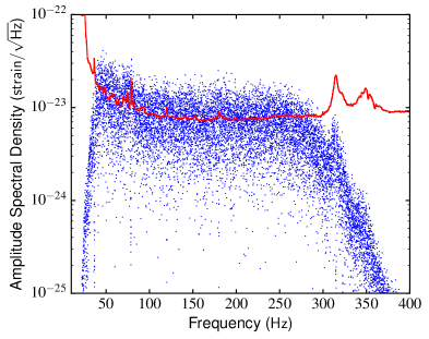
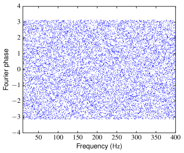
Figure 2: Left panel: normalized magnitude of $\tilde{s}_{cbp}$ (blue) and ASD baseline $\sqrt{S_{b}(f)}$ (red) for Hanford at the time of GW150914. Right panel: phase of $\tilde{s}_{cbp}$. (A plot of phase differences of adjacent frequencies looks equally random.)

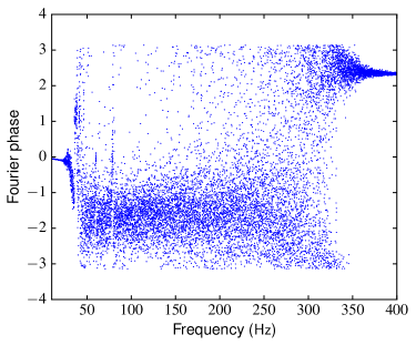
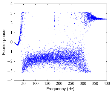
Figure 3: Phase of $\tilde{s}_{cbp}$ for Hanford (left) and Livingston (right) when filtering was performed without using window functions to prevent border distortion.

Order 2 Butterworth notch filters were used to remove the deterministic signals from the 32 s records, $s(t)$, leaving a clean signal, $s_{clean}(t)$, in the pass bands of interest. The filter frequencies and widths were manually adjusted to reduce obvious spectral peaks to the level of the broadband noise. A window with 0.5 s Hann end tapers was used to avoid border distortion. Throughout this work, time-domain filters were applied forward and backward to nullify any phase change. Finally, noise outside the band of interest was suppressed by a band pass filter, yielding $s_{cbp}(t)$. The pass band was adjusted for each event to optimize the signal extraction, with extreme bounds of 35 Hz and 315 Hz for the studied events. Figure 2 shows the magnitude and phase of $\tilde{s}_{cbp}$ for GW150914 at Hanford, where $\tilde{s}$ is the discrete Fourier transform of $s$ and the amplitude is normalized to match the total power of $s_{cbp}$. Equivalent plots for Livingston and for the other events are very similar.

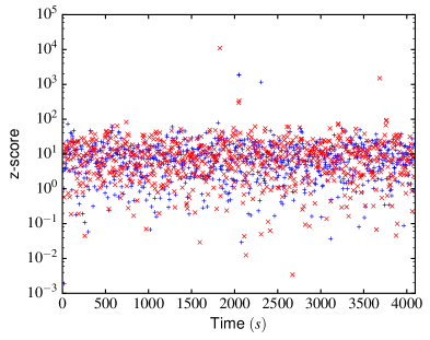
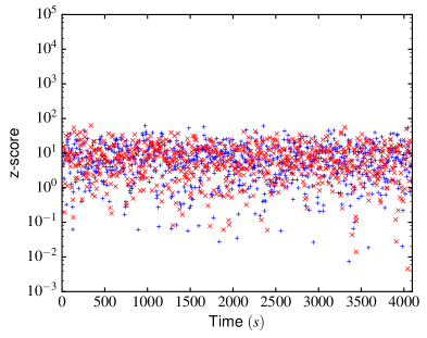
Figure 4: Left panel: GW150914 - z-scores from normaltest of measured noise for Hanford (blue $+$) and Livingston (red $\times$). Right panel: equivalent z-scores for band-passed Gaussian noise.

Doing the above signal cleaning without the use of smoothly tapered window functions to avoid border distortion gives similar spectral amplitudes, but the phase plots, shown in Figure 3, are no longer random. Comparison of these latter plots with similar plots in ref. [17] reveals great similarity. It thus appears that the authors of [17] may not have used suitable window functions. The effects of border distortion are also apparent elsewhere in [17], to the extent that the reliability of the findings and conclusions of that work must be questioned.

Although we do not give the specifics in every case, window functions have been applied wherever warranted in the work reported here. For each situation, window parameters have been chosen to avoid border distortion effects while minimizing bias of useful information.

Statistical tests were performed on the long records for each of the four events. First, 255 overlapping 32 s records were drawn from each of the long records. These short records were cleaned, band-pass filtered, and whitened by scaling in the frequency domain by $\sqrt{N/S_{b}(f)}$ (where $N$ is arbitrarily chosen as the mean of $S_{b}(f)$ in the 3rd quartile of the pass band). Then three overlapping 8 s records were drawn from the central 16 s of the processed 32 s records, avoiding window effects on the ends of the 32 s records. Each 8 s record was tested for normality using the z-score of D’Agostino and Pearson, which gives a combined measure of skew and kurtosis [19, 20, 21]. Figure 4 shows the z-scores for all the 8 s records drawn from the GW150914 data. Also shown is a plot where the data was randomly generated with a normal distribution, band-pass filtered with the same pass band as the real data (and using the same window function), and then subjected to the same ‘normaltest’. High z-score values from the measured data correspond to obvious glitches in one detector or the other, and to the detected event at both detectors. Otherwise, the measured and randomly generated data have similar z-scores.

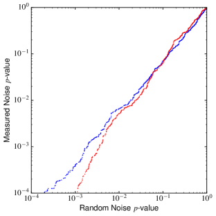
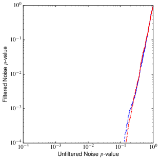
Figure 5: Top panel: sorted $p$-values of cleaned, band-passed and whitened noise records from Hanford (blue) and Livingston (red), plotted against sorted $p$-values of similarly band-passed Gaussian noise records. Each $p$-value estimates the likelihood that the 32768 samples in a record have been generated by a Gaussian random process. Bottom panel: a similar plot showing $p$-values for band-passed versus unfiltered Gaussian noise records.

The normaltest also generated $p$-values for the null hypothesis that the data comes from a normal distribution. As the number of normally distributed samples in a record becomes infinite, the $p$-value should go to 1. But a set of finite length records, even if all samples are generated by a Gaussian (pseudo-)random process, will have a distribution of $p$-values less than 1. Figure 5 compares the $p$-value distributions for the filtered and whitened measured strain records and the filtered, randomly generated records. The lower panel demonstrates that unfiltered records of Gaussian random noise tend to have significantly higher $p$-values than similar records that have been band-pass filtered in the same way as the GW150914 data. The (filtered) measured data is just slightly less likely to be identified as Gaussian than is the band-passed Gaussian noise, with Livingston having somewhat larger reductions than Hanford.

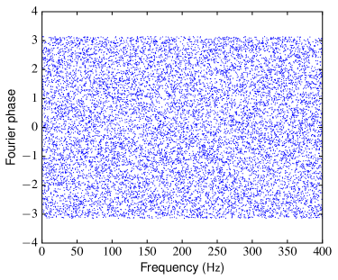
Figure 6: Phase from Fourier transform of the sum of cross-correlations between Hanford and Livingston for 255 overlapping, cleaned and filtered 32 s records drawn from each of the 4096 s records for GW150914.

A final test looked for correlations between the two detectors. The cross-correlations between detectors for all 255 overlapping, cleaned and filtered 32 s records drawn from the 4096 s record for GW150914 were summed. Fig. 6 shows phases from the Fourier transform of this composite cross-correlation; there are no significant features in the magnitude spectrum. The apparent randomness of the phases is consistent with the absence of correlations between the broadband noise at the two detectors.

3 Signal extraction

The techniques used by LIGO to detect and characterize black hole coalescence signals tell us at what time the events appear in the data records $s(t)$ and yield template waveforms $H(t)=\mathfrak{h}_{p}(t)+i\mathfrak{h}_{c}(t)$ that fit the observations reasonably well. In the following sub-sections we describe how, using the approximate event time and approximate time-dependent frequency content of the template, we extract from the records $s(t)$ much cleaner representations $s_{f}(t)$ of the gravitational strain waveforms and the associated uncertainties. (The full template waveform is used at the outset to determine the approximate signal time offset between sites, but subsequent iterative analysis obviates influence of the template’s detailed phase and amplitude information.) We also describe how our method is adapted, in the case of a strong signal like GW150914, to obtain a clean strain waveform without using a template, but simply assuming the signal has the smoothly varying frequency content characteristic of a black hole inspiral, merger and ringdown.

The relation of the cleaned strain signals at the two sites to each other and to the template is characterized as follows. Best-fit values are obtained for the difference of signal arrival times:

$$\Delta t_{event}=t^{H}_{event}-t^{L}_{event}\,,$$ (1)

where the superscripts $H$, $L$ refer to the two detectors. The complex templates are fitted to the extracted waveforms to determine, for each detector $D$, the best-fit relative amplitude $A^{D}$ and phase $\phi^{D}$ for the real-valued template:

$$h^{D}=A^{D}\,(\mathfrak{h}_{p}\,\cos{\phi^{D}}-\mathfrak{h}_{c}\,\sin{\phi^{D}})\,.$$ (2)

Unless needed for clarity, the superscripts $D$, $H$, $L$ will often be omitted below. The phase difference $\Delta\phi=\phi^{H}-\phi^{L}$ is also independently determined, without using knowledge of $\phi^{H}$ or $\phi^{L}$.

The extracted waveforms may, and indeed do, differ from the templates. Differences between the signals extracted from the two detectors are used to estimate the residual noise. Statistical analysis supports determination of uncertainties in time offsets, template amplitudes and phases, and residual differences between the extracted signals and the templates.

3.1 Extraction process

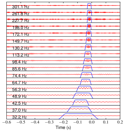
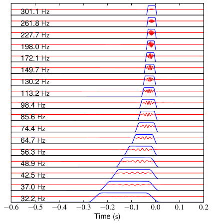
Figure 7: Time-frequency bands for GW150914 derived without use of the template (left) and using the template (right). The red waveforms are the filtered signal $\mathcal{F}_{b_{i}}(s^{L}_{cbpw})$ and template $\mathcal{F}_{b_{i}}(\mathrm{Re}(H_{cbpw}))$, respectively, at the indicated frequencies, $f_{i}$. The corresponding windows $W_{i}$, with Planck tapers, are in blue.

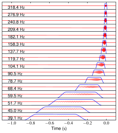
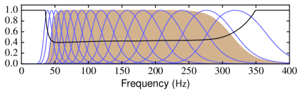
Figure 8: Top panel: Similar to the right panel of Fig. 7, for GW151226. Bottom panel: Filter response amplitudes for GW151226. The light brown background shows the 45 – 315 Hz pass band; the blue lines show the narrow bands of the top panel; and the black line the normalization $1/N(f)$ that compensates for band overlaps.

The signal filtering described in Section 2 eliminates deterministic noise (i.e., spectral peaks) and noise outside the frequency pass band ultimately chosen to best reveal the signal. For the resulting filtered 32 s records, we write

$$s_{cbp}(t)=n(t)+g(t)\,,$$ (3)

where $n(t)$ is band-limited, nearly Gaussian noise and $g(t)$ is a filtered representation of the true gravitational wave at the detector. We expect $g$ to have time-dependent frequency content similar to $H_{cbp}$ (which is the template $H$ filtered the same as $s$ was to obtain $s_{cbp}$). Exploiting this similarity, our strategy is to implement additional filters that selectively reduce all portions of $s_{cbp}$ that are incompatible with the time-dependent frequency content of $H_{cbp}$. This minimizes $n$ to better reveal $g$. In the following, we have arbitrarily chosen Livingston as the reference site. Choosing Hanford, instead, would not have materially changed the results.

Iterative calculations, with too many details to describe here, were necessary to converge on best-fit signal time offsets, amplitudes and phases and extract corresponding signals $s_{f}$. Schematically, the steps followed are:

(i) Reduce time-span: Select, for use in all subsequent steps, 4 seconds of cleaned, band-passed data starting 2.8 s before the nominal event time. Do this for the template also. All of the studied events have duration and usable bandwidth that ensures observations outside this time window will contribute only to $n(t)$.

(ii) Synchronize signals: Cross-correlate the filtered template $H^{D}_{cbp}$ and signal $s^{D}_{cbp}$, for each $D$, to find the time of best match. Interpolate, using a quadratic fit in the neighborhood of the peak, to achieve time resolution finer than the $1/4096$ s data time steps. Using $s^{L}_{cbp}$ as reference, time-shift $s^{H}_{cbp}$ and $H^{D}_{cbp}$ so all these signals become coincident. For GW150914, cross-correlation between $s^{H}_{cbp}$ and $s^{L}_{cbp}$ was sufficient to determine their relative time offset.

(Synchronization was also done using whitened waveforms $s_{cbpw}$ and $H_{cbpw}$ instead of $s_{cbp}$ and $H_{cbp}$, where the whitening was performed in the frequency domain by multiplying by $\sqrt{N/S_{b}(f)}$ as described in Section 2. Differences between the results with and without whitening were not significant.)

(iii) Choose time-frequency (t-f) bands: Define overlapping, narrow frequency bands

$$b_{i}=(f_{i}/1.15,f_{i}\times 1.15),~{}~{}f_{i+1}=f_{i}\times 1.15$$ (4)

that span the frequency pass band chosen for the event. The ratio 1.15 was chosen to divide the signal into about 16 bands. No attempt was made to optimize this ratio — decreasing it would increase the computational cost, while increasing it significantly would result in less effective noise rejection. Using each $b_{i}$, apply a Butterworth band pass filter $\mathcal{F}_{b_{i}}$ to $H_{cbpw}$ (or, for template-independent analysis, to $s_{cbpw}$). In simplified form, the algorithm for choosing the time windows is as follows. For each $i$, find the contiguous time window $W_{i}$ surrounding the maximum of the envelope of $\mathcal{F}_{b_{i}}(H_{cbpw})$ (or of the autocorrelation of $\mathcal{F}_{b_{i}}(s_{cbpw})$) and extending to $1/2$ of the maximum (or an inflection point). Symmetrically scale the width of $W_{i}$ by the parameter $\alpha$, which is tuned for each event. (When using $s_{cbpw}$, time-shift $W_{i}$ so it encloses the peak of the envelope of $\mathcal{F}_{b_{i}}(s_{cbpw})$.) Finally, add a Planck taper to each end of $W_{i}$, further increasing the total non-zero window length by 50%.

Choosing narrower time windows rejects more noise at the expense of increased signal distortion — this proved beneficial for events with weak signals. The values chosen for $\alpha$ were $1.7$ for GW150914 and GW170104, $1.3$ for LVT151012, and $1.215$ for GW151226. We discuss $\alpha$ further in Section 4.

Figure 7 shows the resulting windows $W_{i}$ for GW150914 computed without and with use of the template. The upper panel of Figure 8 shows the $W_{i}$ for GW151226, computed using the template.

(iv) Apply t-f bands: For each $i$, and each detector, construct the narrowly filtered waveform $s_{i}=\mathcal{F}_{b_{i}}(s_{cbp}\times W_{i})$, and its Fourier transform $\tilde{s}_{i}$. Sum the $\tilde{s}_{i}$ to give a composite frequency-domain representation:

$$\tilde{s}_{f}=\frac{1}{N(f)}\sum\limits_{i}{\tilde{s}_{i}}\,,$$ (5)

where $1/N(f)$ compensates for overlapping bands. The lower panel of Figure 8 shows the amplitude response functions of the individual filters $\mathcal{F}_{b_{i}}$ for GW151226 and the corresponding $1/N(f)$. Transform back to the time domain to obtain the filtered signals $s^{H}_{f}$ and $s^{L}_{f}$. Apply the t-f bands to the template in the same way to obtain $H^{H}_{f}$ and $H^{L}_{f}$, where the $H$-$L$ distinction arises due to the different spectral peaks at the two detectors.

(v) Match phases and amplitudes: Having already made $s^{H}_{f}$, $H^{H}_{f}$ and $H^{L}_{f}$ synchronous with $s^{L}_{f}$, find, for each detector, the phase $\phi^{D}$ and amplitude $A^{D}$ that yield from $H^{D}_{f}$ a real template $h^{D}_{c}$ that best matches $s^{D}_{f}$. (See Eq. (2).) The desired phase is the angle in the complex plane at which the cross-correlation of $s^{D}_{f}$ and $H^{D}_{f}$ has maximum amplitude. As done for precise time offsets, interpolate to determine a precise phase. The unscaled, phase-coherent real template is then

$$h^{D}_{f}=Re\left(H^{D}_{f}\exp(i\phi^{D})\right)\,.$$ (6)

Finally, $h^{D}_{c}=A^{D}\,h^{D}_{f}$, where $A^{D}$ is given by

$$A^{D}=\frac{s^{D}_{f}\cdot h^{D}_{f}}{h^{D}_{f}\cdot h^{D}_{f}},$$ (7)

with $a\cdot b=\sum{a_{i}b_{i}}$ the inner product of the two waveforms.

The template-dependent phase and amplitude relating $s^{H}_{f}$ to $s^{L}_{f}$ are given by $\Delta\phi=\phi^{H}-\phi^{L}$ and $A^{LH}=A^{L}/A^{H}$. Use these to obtain $s^{H}_{c}=A^{LH}R(s^{H}_{f},\Delta\phi)$, where $R(s,\phi)$ shifts the phases of all Fourier components of $s$ by the angle $\phi$. By construction, $s^{H}_{c}$ (approximately) matches $s^{L}_{c}$ and $h^{L}_{c}$ in time, phase and amplitude, where $s^{L}_{c}\doteq s^{L}_{f}$.

For the template-independent analysis of GW150914, $s^{H}_{f}$ and $s^{L}_{f}$ are directly compared to find $\Delta\phi$ and $A^{LH}$. To do this, construct from $s^{H}_{f}$ a complex signal $S^{H}_{f}=s^{H}_{f}+i\,R(s^{H}_{f},\pi/2)$. Then cross-correlate $s^{L}_{f}$ and $S^{H}_{f}$, and apply the same algorithm as for the template, above, to determine the phase and amplitude that, when applied to $S^{H}_{f}$, will yield $s^{H}_{c}$ that best matches $s^{L}_{c}\equiv s^{L}_{f}$.

The above steps yielded time offsets, amplitudes and phases that can transform the original, unfiltered inputs $s^{D}$ and $H$ into new, “coherent” signals ${s^{\prime}}^{D}$ and $H^{\prime}$ that are approximately time and phase coherent, and have approximately equal amplitudes, with ${s^{\prime}}^{L}\equiv s^{L}$ as reference. Iterative processing, using the above steps but with ${s^{\prime}}^{D}$ and $H^{\prime}$ as input, provides significant but rapidly diminishing corrections to the approximate results.

Table 1: Parameters and results for each event. Definitions and calculation methods are given in Section 3. The frequency pass bands were manually adjusted based on quality of fit. The “true signals” for simulated events have the event times, amplitudes and phases found for the actual events. Uncertainties represent the $\pm 1$-sigma range of results from the simulated events.

    Event GW150914 GW150914 LVT151012 GW151226 GW170104 Template used no yes yes yes yes Pass band  [Hz] 37 to 290 37 to 290 38 to 300 45 to 315 35 to 290 Time diff. (H-L)  $\Delta t_{event}$ [ms] $7.09^{+.20}_{-.09}$ $7.11^{+.21}_{-.09}$ $-0.8^{+.6}_{-.6}$ $0.6^{+.8}_{-.3}$ $-3.1^{+.5}_{-.2}$ Phase diff.  $\phi^{H}-\phi^{L}$ [rad.] $2.94^{+.22}_{-.27}$ $2.95^{+.21}_{-.27}$ $2.7^{+.5}_{-.5}$ $2.4^{+.5}_{-.4}$ $3.2^{+.4}_{-.4}$ H ampl.  $10^{3}\,A^{H}$ $1.30^{+.34}_{-.35}$ $1.35^{+.30}_{-.44}$ $0.7^{+.3}_{-.5}$ $1.4^{+0.6}_{-1.0}$ $0.7^{+.2}_{-.3}$ L ampl.  $10^{3}\,A^{L}$ $1.11^{+.29}_{-.27}$ $1.11^{+.23}_{-.37}$ $0.7^{+.3}_{-.4}$ $1.5^{+0.9}_{-1.0}$ $0.6^{+.2}_{-.2}$ Corr. coef.  $r(s_{w},h_{coh})$ $0.985^{-.007}_{-.104}$ $0.980^{-.006}_{-.113}$ $0.90^{-.05}_{-.30}$ $0.86^{-.02}_{-.24}$ $0.93^{-.01}_{-.19}$ SNR  $\rho_{ci}$ $9.4^{-3.1}_{-5.1}$ $7.1^{-1.4}_{-3.1}$ $1.9^{+0.5}_{-0.3}$ $2.3^{-0.2}_{-0.7}$ $3.5^{-0.5}_{-1.3}$ SNR  $\rho_{ti}$ $9.1^{-1.9}_{-5.6}$ $6.9^{-0.7}_{-4.0}$ $1.7^{+0.8}_{-1.1}$ $1.9^{+0.7}_{-1.4}$ $3.2^{+0.0}_{-1.8}$ SNR  $\rho^{H}_{tr}$ $5.9^{-2.2}_{-4.3}$ $5.3^{-1.8}_{-3.9}$ $1.9^{-0.4}_{-1.5}$ $1.7^{-0.1}_{-1.3}$ $2.0^{-0.3}_{-1.3}$ SNR  $\rho^{L}_{tr}$ $4.0^{-1.1}_{-2.6}$ $3.3^{-0.6}_{-2.2}$ $1.0^{+0.4}_{-0.6}$ $1.0^{+0.4}_{-0.7}$ $2.0^{+0.0}_{-1.2}$ SNR  $\rho_{tc}$ $5.5^{-1.4}_{-3.8}$ $4.9^{-1.2}_{-3.5}$ $2.0^{-0.3}_{-1.6}$ $1.6^{+0.1}_{-1.2}$ $2.5^{-0.3}_{-1.7}$ SNR  $\rho_{tw}$ $5.6^{-1.5}_{-3.9}$ $5.0^{-1.2}_{-3.6}$ $2.1^{-0.4}_{-1.7}$ $1.7^{+0.0}_{-1.3}$ $2.5^{-0.3}_{-1.7}$    

3.2 Signal comparisons

Comparing the waveforms $s^{H}_{c}$, $s^{L}_{c}$, $h^{H}_{c}$ and $h^{L}_{c}$ reveals information about residual noise and allows selection of combinations that best represent the gravitational waves.

The difference between $h^{H}_{c}$ and $h^{L}_{c}$ is not significant, so we use their average:

$$h_{coh}=(h^{L}_{c}+h^{H}_{c})/2\,.$$ (8)

Subtracting the template from the signals gives the residuals:

$$r^{D}_{c}=s^{D}_{c}-h_{coh}\,.$$ (9)

We define the (time-domain) template/residual SNR for detector $D$ by

$$\rho^{D}_{tr}=\sigma(h_{coh})/\sigma(r^{D}_{c})\,,$$ (10)

where $\sigma(\cdot)$ denotes rms over the time interval spanned by all the t-f bands. A combined signal, that weights each $s^{D}_{c}$ inversely with the noise indicated by $\sigma(s^{D}_{cbp})$, is:

$$s_{w}=\frac{s^{H}_{c}+r\,s^{L}_{c}}{1+r}\,,$$ (11)

where $r=\sigma(s^{H}_{cbp})/\sigma(s^{L}_{cbp})$. Equally-weighted coherent and incoherent combinations of the detector signals are:

$$s_{coh}=(s^{L}_{c}+s^{H}_{c})/2\,,$$ (12)

$$s_{inc}=(s^{L}_{c}-s^{H}_{c})/2\,.$$ (13)

For detectors with uncorrelated noise and similar true signals $g$, $s_{inc}$ should be noise-dominated. It is reasonable to expect noise at a similar level to $s_{inc}$ to be hidden in $s_{coh}$ and $s_{w}$, and in the coherent and weighted residuals:

$$r_{coh}=s_{coh}-h_{coh}\,,$$ (14)

$$r_{w}=s_{w}-h_{coh}\,.$$ (15)

Thus, in the SNR values defined below, $\sigma(s_{inc})$ should be interpreted as a proxy for the rms value of the hidden coherent noise.

New SNR definitions follow from the above:

$$\rho_{tw}=\sigma(h_{coh})/\sigma(r_{w})\,,$$ (16)

$$\rho_{ti}=\sigma(h_{coh})/\sigma(s_{inc})\,,$$ (17)

$$\rho_{tc}=\sigma(h_{coh})/\sigma(r_{coh})\,,$$ (18)

$$\rho_{ci}=\sigma(s_{coh})/\sigma(s_{inc})\,.$$ (19)

The above SNR values measure, in slightly different forms, the strength of the extracted signals or scaled templates relative to detector noise or computed residuals. They are mathematically and conceptually distinct from the matched-filter detection SNRs, reported in the discovery papers [1, 2, 3, 4, 5, 6, 7]. Section 4.1 has further remarks regarding these different ways of measuring SNR.

For a measure of the overlap between the extracted signal and template we compute the Pearson correlation coefficient:

$$r(s_{w},h_{coh})=\frac{s_{w}\cdot h_{coh}}{\sqrt{(s_{w}\cdot s_{w})(h_{coh}\cdot h_{coh})}}.$$ (20)

Before presenting results, we will describe the use of simulations to validate and statistically characterize our signal extraction methodology.

3.3 Simulations

For each analyzed event, inserting the best fit amplitude $A^{D}$ and phase $\phi^{D}$ into Eq. (2) yields the real-valued template $h^{D}$ for the unfiltered gravitational wave signal at site $D$. Simulated event records $q^{D}$ were created by adding $h^{D}$ to each of 252 overlapping 32 s noise records drawn from the 4096 s record $s^{D}_{l}$ (avoiding the time of the actual event). Each pair $(q^{H},\,q^{L})$ was then processed in exactly the same way as the records containing the real event. However, instead of being individually tuned, all the simulated events used the same pass band and the same width parameter for t-f bands as were used for the corresponding real event.

The weighted waveforms $q_{w,i}$, where $i$ indicates the simulation number, extracted from the simulated events can be directly compared to the known injected signal $h_{coh}$. Statistical distributions of parameters determined in the signal extraction process — time offsets, $A^{D}$, $\phi^{D}$, and SNR values —  are indicative of the uncertainties of the parameters found for the real events.

The signal extraction process failed to find an event time offset between detectors within the acceptable $\pm 10$ ms range for 14 of the 1260 simulated events, one failure for each of GW150914 (template not used) and GW151226 and the rest for LVT151012. These were omitted from further analysis. Boosting the injected signal amplitudes by 20% reduced the number of failures to four, by 30% to one, and by 80% to zero.

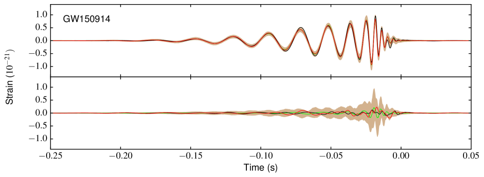
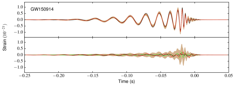
Figure 9: GW150914 without (upper) and with (lower) use of the template. Top panels: weighted combined signal $s_{w}$ (black) and coherently matched template $h_{coh}$ (red), with Livingston as reference. When the template was added to noise records, 90% of the extracted signals $q_{w,i}$ lie within the light brown band. The median of the $q_{w,i}$ signals from the simulations is a green line almost entirely hidden by the red line. Bottom panels: incoherent signal $s_{inc}=\scriptstyle\frac{1}{2}\textstyle(s^{L}_{f}-s^{H}_{f})$ (black) and residual $r_{w}=s_{w}-h_{coh}$ (red). Equivalent residuals for simulated events lie within the light brown band 90% of the time; the green line is the median simulation residual.

3.4 Results

Values of the parameters, correlation coefficients (Eq. (20)), and SNRs (Eqs. (10), (16) – (19)) found for each of the events, with corresponding $\pm 1$-sigma bounds derived from the simulations, are given in Table 1. For the time differences, phase differences, and amplitudes, results for the actual events — which were used as “true” parameter values for the simulations — lie reasonably within the statistical ranges found from simulated events. For the correlation coefficients and SNR values, results from actual events generally lie above the 1-sigma ranges from simulations — we explain why in Section 4.

For GW150914, analyzed both without and with use of the template, extracted waveforms, and bands enclosing 90% of the extracted waveforms from simulations, are shown in Fig. 9. Similar plots for LVT151012, GW151226 and GW170104 are shown in Fig. 10. Time periods when $r_{w}$ and $s_{inc}$ are nearly equal or nearly opposite will have the noise at Hanford or Livingston dominating over the other. Event residuals lie almost completely within the 90% bands obtained from the simulations.

Plotted as green lines in the upper panels, the median values of the extracted waveforms $q_{w,i}$ from the simulations are almost entirely obscured behind red lines for $h_{coh}$. In the same order as the plots of Fig. 9 and 10, the correlation coefficients between $h_{coh}$ and the simulation medians are 0.9983, 0.9997, 0.9918, 0.9968, and 0.9987. This indicates that the extraction process gives an unbiased (but still noisy) representation of the true gravitational wave signal.

The waveforms $s_{w}$ obtained for GW150914 without and with use of the template are nearly identical, with 0.996 correlation. For all events, the extent of the light brown band in the upper panels seems consistent with the $\pm$ variation of time differences, phase differences, and amplitudes (Table 1). The simulation residuals shown by the light brown bands in the lower panels have high amplitudes near the zero crossings of $s_{w}$, suggesting (known) phase errors as the main cause.

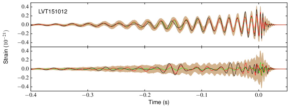
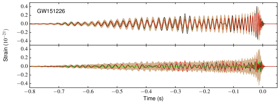
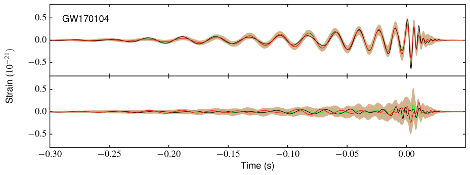
Figure 10: LVT151012, GW151226 and GW170104, all with use of templates. See legend of Fig. 9 for details.

4 Discussion

Matched filters are effective at discovering the occurrence of an expected signal $h$ within a noisy data stream $s$. If $s=g+n$, where the true signal $g$ correlates strongly with $h$, then the matched filter will indicate detection of $h$. However, the matched filter does not distinguish the difference $\delta=g-h$ from the noise.

In this work, the existence, times and basic characteristics of the reported gravitational wave signals have been taken as given — prior knowledge. Working with data provided by the LOSC, we have developed a filtering strategy to preferentially reduce $n$ but not $g$, thereby making the filtered signal $s_{f}$ a better representation of $g$. This was done without imposing specific phase relationships between the different spectral components. However, our assumption that the signal has the characteristic form expected of black hole coalescence — as seen in the templates — imposed the implicit requirement that the phases vary smoothly with frequency.

Our filtering strategy is grounded in the recognition that the true signal $g$ in each narrow frequency band $\Delta f_{i}$ of a black hole coalescence event has significant magnitude only within a brief, contiguous time interval $\Delta t_{i}$. Measured signal $s$ in the band $\Delta f_{i}$ but outside the interval $\Delta t_{i}$ will be dominated by noise. The algorithms we have developed determine suitable t-f bands directly from the observed, sufficiently strong signal (GW150914) or from a reasonable-fit template provided by LIGO. The bands overlap in both frequency and time to ensure almost all of the true signal is maintained in the filtered result. Normalization compensates for band overlaps, ensuring that no spectral component of the output has weight greater than one. By adjusting the width of the time windows, using parameter $\alpha$, noise rejection can be balanced against distortion of the true signal (and template). Choosing large $\alpha$, for strong signals, gives time windows that include almost all true signal energy. Choosing a smaller $\alpha$, for weak signals, accepts some filtering of true signal in order to increase noise suppression. However, Fig. 8 shows that even the smallest value, $\alpha=1.215$, preserves most of the signal.

Correlation coefficients $r(q_{w,i},h_{coh})$ for the simulated events were generally smaller than $r(s_{w},h_{coh})$ for actual events. To explain this, we note that the templates $H$, provided by LIGO, are particularly good matches for the observed strains $s^{D}=n^{D}+g^{D}$, which differ from the true signals $g^{D}$. If the $g^{D}$ could be known, then applying the LIGO analysis process to simulated signals $q^{D}_{i}=n^{D}_{i}+g^{D}$ would lead to many different templates $H_{i}$, each tailored to the unique noise $n^{D}_{i}$. But in our simulations the true $g^{D}$ are not known. As a proxy, we have used instead $h^{D}$, derived from $H$ and thus tainted by $n^{D}$ at the time of the actual event. The difference $g^{D}-h^{D}$ is not ignorable. The result is that waveforms $q_{w,i}$ extracted from the simulated signals tend to not match $h_{coh}$ as well as $s_{w}$ does.

Since we have no evidence that the (unknown) noise $n^{D}$ at the time of the actual event is statistically different from the noise samples $n^{D}_{i}$, the distribution of extracted waveforms $q_{w,i}$ obtained from the simulations should be taken as a good indication of the uncertainty with which $h_{coh}$ (and $s_{w}$) represent $g$. Because, for simulation of a given event, the same signal $h^{D}$ was injected into each noise sample $n^{D}_{i}$, the median of the $q_{w,i}$ should closely match $h_{coh}$, as seen in Figures 9 and 10. For the same reason, the distributions of simulation results for the time offset, phase and amplitude parameters should have mean values that closely approximate the corresponding parameters for the actual events, from which the $h^{D}$ were constructed. The noise that gives these distributions their widths also makes uncertain the true values of the parameters, and hence the means of the distributions that would result if $h_{coh}$ corresponded precisely to $g$. For each given parameter, the uncertainty of the mean stems from the same noise, and will thus have the same distribution, as the parameter values obtained from simulations. This implies that uncertainties of the true parameter values have bands $\sqrt{2}$ wider than indicated by the $\pm 1$-sigma ranges from the simulations.

4.1 Remarks on SNR

We have defined SNRs (Eqs. (10), (16)–(19)) that are ratios of rms amplitudes of filtered time series records that serve as proxies for the true signal and true noise. Computed in the time domain, these are sometimes referred to as instantaneous SNRs. Results for the studied events are shown in Table 1.

For GW150914, slightly higher SNR values for the signal extraction without, as opposed to with, use of the template can be attributed to the somewhat greater noise exclusion by narrower time windows for the t-f bands, evident in Fig. 7. This difference is also seen in the correlation coefficients, but there is no significant difference in the obtained signal parameters.

For all events but LVT151012, the values of $\rho_{ci}$ and $\rho_{ti}$, with $\sigma(s_{inc})$ in the denominator, are higher than the other SNR measures, which use residuals as proxies for noise. This can be traced to contributions $g-h$ to the residuals, that become relatively more important when the detector noise (for which $s_{inc}$ is a proxy) is small.

More notably, SNR values for simulated events tend to be lower than for actual events, just as with correlation coefficients. Again, the main explanation is that the template $H$, provided by LIGO, is a statistically better match for the observed strains $s^{D}=g^{D}+n^{D}$ than it is for the (unknown) true strains $g^{D}$, thus giving anomalously high SNRs. For the simulated signals, the injected signal $h^{D}$ is derived directly from $H$ and there is nothing to make the template match $q^{D}_{i}=h^{D}+n^{D}_{i}$ better than it does $h^{D}$. The SNRs from simulations should thus be considered a more reliable representation of the truth.

We further observe that although $n^{D}$ makes a tainting contribution to $s_{w}$ and $H$, this will not significantly diminish the coherent component of noise that is complementary to $s_{inc}$ (or $q_{inc,i}$) and which we have assumed has rms value similar to $\sigma(s_{inc})$.

The instantaneous SNRs discussed above are distinct in definition, purpose and interpretation from a matched-filter SNR. The matched-filter SNR $\rho$, used by LIGO to quantify the match between a test template $(\mathfrak{h}_{p},\mathfrak{h}_{c})$ and a noisy measured signal $s$, for a given detector, is defined by [22, 4]:

$$\rho^{2}(t)=[\langle s|\mathfrak{h}_{p}\rangle^{2}(t)+\langle s|\mathfrak{h}_{c}\rangle^{2}(t)]\,.$$ (21)

Here, the optimally normalized correlation between $s$ and each template component, $\mathfrak{h}_{p}$, $\mathfrak{h}_{c}$, offset in time by $t$, is defined by:

$$\langle s|\mathfrak{h}\rangle(t)=4\,\Upsilon\,\mathrm{Re}\int_{0}^{\infty}\frac{\tilde{s}(f)\tilde{\mathfrak{h}}^{*}(f)}{S_{n}(f)}e^{2\pi ift}df\,,$$ (22)

where $S_{n}(f)$ is the positive frequency PSD of the detector noise, and $\Upsilon$ is a normalization factor. For each detector, $\Upsilon$ is chosen such that for an ensemble consisting of many distinct realisations of the detector noise $s$ (with no signal), taken from the time interval used to determine $S_{n}(f)$, the ensemble averages of $\langle s|\mathfrak{h}_{p}\rangle^{2}=\langle s|\mathfrak{h}_{c}\rangle^{2}=1$, independent of $t$. With no signal present, Eq. (21) then gives the (time-independent) expected value $<\!\rho^{2}\!>\,\,=2$.

A gravitational wave event adds real signals $g$ to the noise at each of the detectors, resulting in peaks $(\rho^{2})^{H}$, $(\rho^{2})^{L}$ of $\rho^{2}(t)$ at times $t^{H}\!,\,t^{L}$ separated by not more than the light travel time between detectors. Combining the peak $\rho$ values from the two detectors in quadrature gives the event SNR:

$$\rho_{ev}=\sqrt{(\rho^{2})^{H}+(\rho^{2})^{L}}\,.$$ (23)

The $\rho_{ev}$ values published by LIGO for the four events studied here are [4, 5]:

GW150914	–	23.7
LVT151012	–	9.7
GW151226	–	13.0
GW170104	–	13.

These values represent the collective result of analysis with many different templates, each corresponding to different physical parameter values $\theta$, and the requirement for detection of similar signals at both detectors with sufficiently small time offset. As described in [22], maximum-likelihood parameter values $\theta_{ML}$ and uncertainties have been estimated by comparing Bayesian evidence for a wide range of plausible parameter values. The template $h[\theta_{ML}]$ corresponding to $\theta_{ML}$ then maximizes the event SNR. For GW150914, instead of the 23.7 cited above, consideration of a finer sample space for $\theta$ gave $\rho_{ev}[\theta_{ML}]=25.1^{+1.7}_{-1.7}$ [12].

The precise values of matched-filter SNRs obtained using Eqs. (21) and (22), and the likelihoods obtained in the Bayesian analysis, will always depend on the actual noise $n_{a}$ realized during the time interval $(t_{0}-\Delta t,t_{0})$ when the signal $g$ has significant amplitude. Different noise will yield different SNRs. To demonstrate this, we have computed $\rho_{ev}$, as defined by Eq. (23), for each of the studied events. Using the LIGO-provided templates $(\mathfrak{h}_{p},\mathfrak{h}_{c})$, we found slightly lower $\rho_{ev}$ values than those listed above. For each of the events, we then injected the same signal $h$ (our best fit) into many different noise realizations $n_{i}$ (as in our simulations), and found that matched-filter SNRs $\rho_{ev,i}$ for the template $(\mathfrak{h}_{p},\mathfrak{h}_{c})$ have variance $\mathrm{var}(\rho_{ev,i})\sim 1$ . The results of our calculations are:

Event	$\rho_{ev}$	$\mathrm{mean}(\rho_{ev,i})$	$\mathrm{var}(\rho_{ev,i})$
GW150914	23.5	24.0	1.04
LVT151012	8.6	8.2	0.83
GW151226	11.2	10.9	1.06
GW170104	12.6	11.8	1.07

SNRs for simulated events at the individual detectors have similar variances: $\mathrm{var}(\sqrt{(\rho^{2})_{i}^{H}})\sim\mathrm{var}(\sqrt{(\rho^{2})_{i}^{L}})\sim 1$. Injecting the same $h$ into noise records that are identical except for relative time shifts as small as 2 ms gives detection SNRs whose variations about the mean are apparently uncorrelated.

For the studied events, the actual data $s=g+n_{a}$ have limited useful bandwidth; and the signal $g$ is detectable only for a brief interval of $\sim\!\!1$ s or less, which is too short to demonstrate the (band-limited) Gaussian nature of the noise. With the limited $1/\Delta t$ frequency resolution afforded by such a brief interval, the fluctuations of $|\tilde{n}_{a}|$ about $\sqrt{S_{n}}$ cannot exhibit the obvious stochastic character exemplified by $\tilde{s}_{cbp}$ (a 32 s record) in the left panel of Figure 2.

To illustrate this, Fig. 11 shows Fourier amplitudes for a 0.4 s period spanning the GW150914 event. The spectrum of the extracted signal $s_{w}$ matches that of the template $h_{cbp}$ (for the same 0.4 s) quite well; differences between them can be attributed to both real differences $\delta=g-h$ and residual coherent noise. The noise in $s_{cbp}$, i.e., what remains after subtracting the signal $s_{w}$, has spectral fluctuations consistent with the 90% band of $|\tilde{n}_{i}|$ obtained by analyzing 252 different 0.4 s noise samples $n_{i}$. The median of the $|\tilde{n}_{i}|$ has much smaller fluctuations, making it similar (except for the imposed pass band) to $\sqrt{S_{b}(f)}$ in Fig. 2.

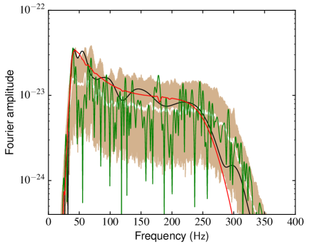
Figure 11: GW150914 Fourier amplitudes. The white line shows the median of $|\tilde{n}_{i}|$ for 252 noise samples $n_{i}$ from Livingston; 90% of the $|\tilde{n}_{i}|$ lie within the light brown band. FFTs were computed using 32 s records, with a smoothly tapered window $W$ masking all but 0.4 s. Amplitudes are scaled by $\sqrt{32/0.3}$ to compensate for $W$ and allow comparison with $\sqrt{S}$. The smooth red line shows the template spectrum, $|\tilde{h}_{cbp}|$, with the same $W$ and scaling. The black line shows $|\tilde{s}_{w}|$ and the jagged green line $|\tilde{n}|$, both also scaled, where $n=(s^{L}_{cbp}-s_{w})\times W$ is the noise filtered out using the t-f bands to obtain $s_{w}$.

The spectra in Fig. 11 have been normalized to achieve a frequency-domain signal power (total energy / 32 s) that matches the mean time-domain power (corrected for window tapers) during the chosen 0.4 s segment of each 32 s record. Every 0.4 s segment of stationary noise should have similar power — so it is not surprising that the median amplitude of $\sim\!10^{-23}$ matches $\sqrt{S_{b}(f)}$ quite well. The correspondence for $|\tilde{s}_{w}|$ and $|\tilde{h}_{cbp}|$ is more subtle. The 0.4 s window was chosen to snugly frame the event. Doubling the window length would have cut the signal and template Fourier amplitudes in half; reducing the length would have excluded portions of the signal and changed the shape of its spectrum. Changing the window length would also have sampled different noise and given a different detailed noise spectrum.

We expect that the above-demonstrated dependence of matched-filter SNR values on the actual detector noise coincident with a black hole coalescence event will apply also to the outcomes of Bayesian parameter estimation. Similar to our use of simulations for estimation of uncertainties, the frequentist approach of injecting the same signal into different noise samples might provide useful guidance on the noise-related uncertainties of estimated physical parameters. At the very least, it would test the assumption that Bayesian and frequentist approaches give similar outcomes.

For the purposes of the present work, matched-filter SNR values indicate the trust that can be placed in the prior knowledge our signal extraction method relies on. Our instantaneous SNR values then indicate how strongly the extracted signal can be made to stand above the residual noise, when the prior knowledge is used to guide the definition of t-f bands for selective filtering. The matched-filter and instantaneous SNR values are thus seen as complementary.

4.2 Comparison with wavelet approaches

Our analysis method, as presently implemented, is limited to the narrow purpose of extracting clean representations of gravitational wave signals from already identified black hole coalescence events. Although, when the signal is weak, we make use of reasonable-fit templates, the prior knowledge we use from the template is only the approximate evolution of frequency over time — to allow selection of t-f bands.

Wavelet based approaches [13, 24] offer flexibility in analyzing a wide variety of gravitational wave signals. Such methods can be used for both signal detection and characterization. Combining wavelet and template based methods can improve parameter estimation and rejection of instrument glitches.

For two events we can give quantitative comparisons. For GW170104, the wavelet based analysis achieved 87% overlap between the maximum-likelihood waveform of the binary black hole model and the median waveform of the morphology-inde-pendent analysis [5]. We found 93% overlap between the LIGO-provided template and the extracted signal $s_{w}$, and 99.87% overlap between the template injected into real noise records and the median waveform extracted from the 252 simulated events. For GW150914, processed without use of the template, our corresponding overlaps are 98.5% and 99.83%, while wavelet analysis achieved a 94% overlap with the binary black hole model [12]. However, as we have noted above, the overlaps with the true gravitational wave signals $g$ are almost certainly lower because the template (or maximum-likelihood) waveforms are tainted by the actual noise at the time of detection.

4.3 Correlation of noise and residuals

It has been argued in [17] that cross-correlations of the residuals at the two detectors have peaks corresponding to the event time offsets for GW150914, GW151226 and GW170104. This was cited as support for the claim “A clear distinction between signal and noise therefore remains to be established in order to determine the contribution of gravitational waves to the detected signals.” For GW150914, correlations due to the calibration lines in the vicinity of 35 Hz were cited as further support.

We have argued in Section 2 that apparent failure to use appropriate window functions casts doubt on the conclusions of [17]. Our analysis indicates, nonetheless, that cross-correlations of residuals may indeed have significant peaks corresponding to the event time offsets — but the origin of these peaks is not correlations between noise at the two detectors. Instead, they arise because the true signal is not identical to the template, and the difference $\delta=g-h$ will be included in both the residuals. Ignoring minor differences between the true signals, and between corresponding templates, at the two sites (after adjusting the Hanford time, phase and amplitude), we can expand the individual site residuals as $r^{D}=n^{D}+\delta$. The weighted residuals (Eq. (15)) then become $r_{w}=w\,n^{L}_{c}+(1-w)n^{H}_{c}+\delta_{c}$, where the subscript $c$ denotes the same processing as used to obtain $s^{D}_{c}$ and the weight $w\sim 0.5$. Since the noise signals $n^{H}$ and $n^{L}$ are independent (and thus randomly correlated), their antisymmetric combination $n_{inc}\doteq s_{inc}=(n^{L}_{c}-n^{H}_{c})/2$ will have similar statistics to, but be independent of, $n_{w}=r_{w}-\delta_{c}$. It follows that, if $\delta_{c}$ is significant, $\sigma(r_{w})>\sigma(s_{inc})$. From the lower panels of Figures 9 and 10 it appears that, for the actual events, $\sigma(r_{w})\simeq\sigma(s_{inc})$. However, the light brown bands show that the simulation residuals can have significantly greater magnitude. We have attributed this to parameter errors (especially phase) in the extracted $q_{w,i}$’s, with attendant contributions to $\delta_{c}$. The common contribution of $\delta_{c}$ to $r^{H}_{c}$ and $r^{L}_{c}$ will inevitably produce a peak at the event time offset in the cross-correlation of residuals, even though $n^{H}_{c}$ and $n^{L}_{c}$ may be randomly correlated.

5 Conclusions

We have introduced a method for extracting, from noisy strain records, clean gravitational wave signals for black hole coalescence events. Our method takes as prior knowledge the existence and timing of the events, established through matched-filter and other techniques by LIGO. For events whose signals cannot be readily detected without matched-filter techniques we also use, as prior knowledge, the approximate time-dependent frequency content of a reasonable-fit template waveform provided by LIGO.

Statistical tests show that, after filtering to remove spectral peaks and restrict the pass band, the recorded signals prior to and following the detected events are similar to band-passed Gaussian noise. There is no evidence of correlation between the two detectors that would indicate a causal connection.

The extracted waveforms, including for GW150914 extracted without using the template, correlate very strongly with the LIGO templates. Simulations, with template-derived signals injected into real noise records and processed the same as the actual events, show that the analysis method is unbiased. But the simulation results give weaker correlation with the template and lower SNR values than the real events. This suggests that the template is tainted by noise at the time of the real event — it matches the real signal plus noise $(g+n)$ better than it does $g$ alone. The simulation results, based on many different stretches of real noise, support more realistic estimates of parameter uncertainties and SNR values for the actual events.

The methods and results presented here are complementary to the matched-filter, wavelet and statistical analyses used by LIGO. Combining these approaches may lead to more robust determination of the physical parameters and uncertainties for black hole coalescence events. Generalizing our methods to different kinds of physical events, and even to very different problems, may also prove fruitful.

References

References

-
[1]
B. P. Abbott, et al.,
Observation of
gravitational waves from a binary black hole merger, Phys. Rev. Lett. 116
(2016) 061102.
doi:10.1103/PhysRevLett.116.061102.
URL https://link.aps.org/doi/10.1103/PhysRevLett.116.061102 -
[2]
B. P. Abbott, et al.,