Determination of Checkpointing Intervals for Malleable Applications

Abstract

Selecting optimal intervals of checkpointing an application is important for minimizing the run time of the application in the presence of system failures. Most of the existing efforts on checkpointing interval selection were developed for sequential applications while few efforts deal with parallel applications where the applications are executed on the same number of processors for the entire duration of execution. Some checkpointing systems support parallel applications where the number of processors on which the applications execute can be changed during the execution. We refer to these kinds of parallel applications as malleable applications. In this paper, we develop a performance model for malleable parallel applications that estimates the amount of useful work performed in unit time (UWT) by a malleable application in the presence of failures as a function of checkpointing interval. We use this performance model function with different intervals and select the interval that maximizes the UWT value. By conducting a large number of simulations with the traces obtained on real supercomputing systems, we show that the checkpointing intervals determined by our model can lead to high efficiency of applications in the presence of failures.

I Introduction

With the development of high performance systems with massive number of processors[1] and long running scalable scientific applications that can use the processors for executions[2], the mean time between failures (MTBF) of the processors used for a single application execution has tremendously decreased[3]. Hence many checkpointing systems have been developed to enable fault tolerance for application executions[4, 5, 6, 7, 8]. A checkpointing system periodically saves the state of an application execution. The application, in the event of a failure, rolls back to the latest stored or checkpointed state and continues execution.

Recent efforts in checkpointing systems are related to the development of parallel applications that can change the number of processors during execution[8, 6]. We refer to these kinds of parallel applications as malleable applications. Malleable parallel applications are highly useful in systems with large number of nodes where the resource availability can vary frequently. In these systems, upon failures of processors used for processor execution, the application can be made to execute on the available processors rather than waiting for the failed processors to be repaired. Malleable applications can also make use of the nodes that become available during execution.

One of the important parameters in a checkpointing system that provides fault tolerance is the checkpointing interval or the period of checkpointing the application’s state. Smaller checkpointing intervals lead to increased application execution overheads due to checkpointing while larger checkpointing intervals lead to increased times for recovery in the event of failures. Hence, optimal checkpointing intervals that lead to minimum application execution time in the presence of failures will have to be determined. Large number of efforts have developed techniques for determining optimal checkpointing intervals[9]. These techniques were primarily developed for sequential applications. They also consider parallel applications where the number of processors used by an application remains constant throughout execution. We refer to these kinds of parallel applications as moldable applications.

In this paper, we develop strategies for determining efficient checkpointing intervals for malleable parallel applications. To our knowledge, ours is the first effort for malleable applications. Our work is based on the work by Plank and Thomason[10] for finding checkpointing intervals and suitable number of processors for executing moldable parallel applications with minimal execution time in the presence of failures. We extend their Markov models to incorporate states and transitions that allow reconfiguration of applications from one processor configuration to another in the event of failures. The states of our Markov model are automatically determined from a specified reconfiguration policy. We use different checkpointing and recovery overheads for different states corresponding to different number of processors. We also define and use a new metric for evaluation of a checkpointing interval for a malleable application, namely, the amount of useful work per unit time (UWT) performed by the application in the presence of failures. Our Markov model is used to estimate the UWT of an application as a function of checkpointing interval. We use this performance model function with different checkpointing intervals and select the interval that maximizes the UWT value. To reduce the modeling time, we have developed techniques for eliminating low probable states and transitions, and parallelized the steps for building the model.

We evaluate the efficiency of our model by using the optimal checkpointing intervals determined by our model in trace-based simulations and finding the total amount of useful work performed by an application in the presence of failures. Our simulations were conducted with large number of failure traces obtained on both dedicated batch systems for a 9-year period on 8 parallel systems and non-dedicated volatile workstations, for three parallel applications, and with three recovery or rescheduling policies. We show that checkpointing intervals determined by our models lead to greater than 80% application efficiency in terms of useful work performed by the application in the presence of failures.

Following are our primary contributions.
1. Developing a model for execution of malleable applications based on the the model by Plank and Thomason for moldable applications. This includes significant extensions to the original model including different definitions for the states of the model, and automatic determination of the states and transition probabilities based on reconfiguration or rescheduling policies.
2. Definition of a new metric for evaluating checkpointing intervals for malleable applications.
3. Optimizing the model by elimination of states and employing parallelism.
4. Extensive simulations with real world failure traces for different applications and with different rescheduling policies.

Section II summarizes the work by Plank and Thomason on modeling moldable applications. Section III describes in detail our model for malleable parallel applications and the metric used for evaluation of checkpointing intervals determined by our model. Section IV explains the optimizations of the model framework. Section V describes the rescheduling policies used by our model. In Section VI, we describe the various simulation experiments we conducted to show the efficiency of the checkpointing intervals determined by our models. Section VII presents related work in the area. Section VIII gives conclusions and Section IX presents future work.

II Background: Checkpoint Intervals for Moldable Applications

The work by Plank and Thomason[10] developed a finite-state Markov chain based performance model to characterize the execution of long running moldable parallel application in the presence of failures. They use the model to find the checkpointing interval, $I$, and the number of processors, $a$, for execution of a long running application in a system with $N$ ($N>a$) processors. Their goal is to minimize the running time of the application in the presence of failures. Spare processors are defined as candidate processors for replacing a processor that failed during application execution. The number of spare processors, $S$, is $N-a$. $L$ is the checkpointing latency or the total time spent for checkpointing and $C$ is defined as the checkpointing overhead or the extra time incurred by the application due to checkpointing. Typically, $C<L$ due to optimizations performed in checkpointing systems. $R$ is the time spent in recovery from a failure. The model assumes exponential distribution for inter-occurrence times of failures and repairs for a processor. $\lambda$ denotes the failure rate and $\theta$ denotes the repair rate for a single processor. Given a trace of failures and repairs of a processor, the mean time to failure (MTTF) of the processor is calculated as the average of times between failures of the processor. The mean time to repair (MTTR) of a processor is calculated as the average of times from when the processor fails to when the processor is available for execution. For a multi-processor system, $\lambda$ and $\theta$ are calculated as the reciprocal of the average of MTTFs and MTTRs, respectively, for all processors.

The Markov chain, $M^{mold}$, consists of three types of states, namely, up, down and recovery, as shown in Figure 1. The application is in an up state if at least $a$ processors are available for execution. If one of the processors used for the execution of the application fails and the total number of functional processors remaining in the system is less than $a$, the application is halted and is considered to be in a down state. The application remains in this state until some of the failed processors are repaired and at least $a$ processors become available for execution again. In this case, the application goes to a recovery state. The application also enters a recovery state from an up state if after the failure of a processor used during the execution, the number of remaining functional processors is at least $a$. In the recovery state, the application tries to recover from the previous checkpoint, spending $R$ seconds for rollback to the checkpointed state, and remains in the recovery state until it creates a new checkpoint after $(I+L)$ seconds. If during the $(R+I+L)$ seconds, none of the processors fail, the application enters an up state and continues execution. If one of the processors fails during the recovery and spares are available for replacement of the failed processor, the application enters another recovery state and restarts the recovery process. However, if spares are not available, the application enters a down state.

Figure 1: States and Transitions for Markov model for moldable applications, $M^{mold}$

The Markov model, $M^{mold}$ consists of $S+1$ up states, $S$ recovery states and $a$ down states. An up state denoted by $[U:s]$, $0\leq s\leq S$, corresponds to application execution on $a$ processors with $s$ spare processors in the system at the time the state is entered. A recovery state denoted by $[R:s]$, $0\leq s<S$, corresponds to application recovery on $a$ processors with $s$ spares available at the start of the recovery. When the application exits an up state due to failure of one of the $a$ processors with $s+1$ spares available, it goes to $[R:s]$ state after replacing the failed processor with one of the $s+1$ spares. After a span of $(R+I+L)$ seconds in a recovery state, $[R:s1]$, the application enters an up state, $[U:s2]$, where $s2$ is the number of spares in the system when the up state is entered. If an application exits an up state due to failure of one of the $a$ processors and the total number of functional processors in the systems is $a-1$, the down state, $[D:a-1]$, is entered. The down state denoted by $[D:p]$, $0\leq p<a$, represents the system with only $p$ processors available. The recovery state, $[R:0]$, is entered from a down state, $[D:a-1]$, after repair of a failed processor resulting in exactly $a$ functional processors.

The probabilities of transitions from the states in $M^{mold}$ are based on the number of functional spares available after the exits of the states. These probabilities are calculated using a birth-death Markov chain, $S^{\tau}$, that helps find the probability of starting with $i$ spares and ending with $j$ spares, $0\leq i,j\leq S$, after $\tau$ seconds. The Markov chain, $S^{\tau}$, consists of $S+1$ states, denoted $[B:s]$, $0\leq s\leq S$, , as shown in Figure 2. Each state, $[B:s]$, corresponds to $s$ functional spares and $S-s$ processors under repair. Transition out of a state $[B:s]$ is either to the state $[B:s-1]$ corresponding to failure of a single processor with probability $s\lambda$ or to $[B:s+1]$ corresponding to repair of a processor with probability $(S-s)\theta$. The states are numbered $1$ to $S+1$ from left to right such that state $i$ represents $S-i+1$ functional spares.

Figure 2: Birth-Death Markov Chain $S^{\tau}$

A $(S+1)\times(S+1)$ square matrix, R, of instantaneous probabilities is defined as:

$${\bf R}=\begin{bmatrix}-S\lambda&S\lambda&\cdots&0&0\\ \theta&-((S-1)\lambda+\theta)&\cdots&0&0\\ \vdots&\vdots&\vdots&\vdots&\vdots\\ 0&0&\cdots&-(\lambda+(S-1)\theta)&\lambda\\ 0&0&\cdots&-S\theta&S\theta\\ \end{bmatrix}$$ (1)

The matrix R is used to calculate a $(S+1)\times(S+1)$ matrix, ${\bf Q}^{S,\tau}=[q_{i,j}^{S,\tau}]$, shown in Equation 2, where the $[i,j]$ entry is the probability that the Markov chain $S^{\tau}$ starting in state $i$ enters state $j$ after $\tau$ seconds. Thus $q_{S-i+1,S-j+1}^{S,\tau}$ is the probability of starting with $i$ functional spares and ending with $j$ spares after $\tau$ seconds.

$${\bf Q}^{S,\tau}=expm({\bf R}\tau)$$ (2)

$expm({\bf R}\tau)$ is the matrix exponential of ${\bf R}\tau$.

If $f_{\tau}$ is the probability density function of the TTF (time to failure) random variable $\tau$, the likelihoods of transitions between the states in $S^{\tau}$ are given by the $(S+1)\times(S+1)$ matrix:

$$[q_{ij}^{S}]=\int_{t}{\bf Q}^{S,t}f_{\tau}(t)dt$$ (3)

The transition probabilities in the original Markov model, $M^{mold}$, are calculated using the ${\bf Q}^{S,\tau}$ and $[q_{ij}^{S}]$ matrices of the birth-death Markov chain, $S^{\tau}$. We illustrate the calculations for probabilities of transitions from the recovery states. For successful transitions from recovery to up states in $M^{mold}$, a failure must not occur within $\delta=R+I+L$ seconds. The probability of no active processor failure during the interval $[0,\delta]$ is $e^{-a\lambda\delta}$. The probabilities of the specific up states after transitions are given by ${\bf Q}^{S,\delta}$, obtained by substituting $\delta$ for $\tau$ in Equation 2. Thus, the probability of transition from $[R:i]$ to $[U:j]$ is $(e^{-a\lambda\delta})(q_{S-i+1,S-j+1}^{S,\delta})$. The probability of an active processor failure within $\delta$ seconds is $1-e^{-a\lambda\delta}$. The failure results in a transition to a recovery state or the down state $[D:a-1]$ depending on the number of spares. The probability density function of the TTF random variable $\tau$ is $a\lambda^{-a\lambda\tau}$ and is conditioned on $\tau$ being in the interval $[0,\delta]$. Thus substituting $f_{\tau}(t)=\frac{a\lambda^{-a\lambda t}}{1-e^{-a\lambda\delta}}$ in Equation 3 and integrating over the interval $[0,\delta]$, the matrix of likelihoods, ${\bf Q}^{Rec,S}=[q_{ij}^{Rec,S}]$, of transitions between the states in $S^{\tau}$ is calculated. The probability of a transition from $[R:i]$ to $[R:j]$ in $M^{mold}$ is then $(1-e^{-a\lambda\delta})q_{S-i+1,S-j+1}^{Rec,S}$ and to $[D:a-1]$ is $(1-e^{-a\lambda\delta})q_{S-i+1,S+1}^{Rec,S}$. Similar calculations are used to find the transition probabilities from the up and down states and are explained in [10]. For finding the transition probabilities from the up states, the matrix of likelihoods, ${\bf Q}^{Up,S}=[q_{i,j}^{Up,S}]$, is used. ${\bf Q}^{Up,S}$ is calculated by substituting $f_{\tau}(t)=a\lambda e^{-a\lambda t}$ in Equation 3 and integrating over the interval $[0,\infty]$. The integral equations for the calculations of transition probabilities from the up and recovery states, using Equation 3, are solved by computing the eigen values and eigen vectors of the ${\bf R}$ matrix, shown in Equation 1. These solutions are also described in detail in [10]. The calculated probabilities of transitions in $M^{mold}$ are represented by a square matrix, ${\bf P}^{mold}$, with the number of rows or columns equal to the total number of up, recovery and down states, and row of ${\bf P}^{mold}$ corresponds to a state of $M^{mold}$ such that $P_{i,j}^{mold}$ is the probability of transition from state $i$ to state $j$ in $M^{mold}$.

Each transition, $i,j$, in $M^{mold}$ is also weighted by $U_{i,j}$, the average amount of useful time or uptime spent by the application in the state corresponding to the start of the transition and $D_{i,j}$, the non-useful or down time spent by the application in the state. The uptime is the time spent by the application performing useful work and is equal to the failure-free running time of the application not enabled with checkpointing. The down time includes the time spent in checkpointing, $C$, recovery, $R$, recomputation of work lost due to a failure, and the time spent in the down states. For example, for a transition from a recovery state $[R:i]$ to an up state $[U:j]$, the useful time, $U_{i,j}=I$ and the down time, $D_{i,j}=R+L$. For a transition to another recovery state, $[R:j]$, a failure must have occurred within the $\delta$ seconds. Thus, the useful time, $U_{i,j}=0$ and the down time, $D_{i,j}=\frac{1}{a\lambda}-\delta\frac{e^{-a\lambda\delta}}{1-e^{-a\lambda\delta}}$, the MTTF (mean time to failure) conditioned on failure within $\delta$ seconds. The useful and down times for the other transitions are calculated similarly and are shown in the work by Plank and Thomason[10]. Thus square matrices, ${\bf U}$ and ${\bf D}$ are constructed corresponding to the transition matrix, ${\bf P}^{mold}$.

The long-run properties of $M^{mold}$, where $M^{mold}$ is taken through a large number of transitions, are used to find the long-run probability of the occupancy of state $i$. This is given by the entry $\pi_{i}$ in the unique solution of the matrix equation, $\Pi=\Pi{\bf P}^{mold}$. If $M^{mold}$ is taken through $n$ transitions randomized according to the transition probabilities, and if $n_{i}$ is the number of occurrences of state $i$ during those transitions, then

$$\pi_{i}=\lim_{n\to\infty}\frac{n_{i}}{n+1}$$ (4)

Since each visit to state $i$ is followed by probabilistic selection of an exit transition, the limiting relative frequency of occurrence of transition $i\rightarrow j$ is the joint probability $\pi_{i}P^{mold}_{i,j}$. Thus, for a long-running task, $U_{i,j}\pi_{i}P^{mold}_{i,j}$ and $D_{i,j}\pi_{i}P^{mold}_{i,j}$ are the expected contributions of useful and non-useful times, respectively, due to the relative frequency of transition $i\rightarrow j$. The availability, $A_{a,I}$, for a given number of processors, $a$, used for execution and a given checkpointing interval, $I$, is the ratio of the mean useful time spent per transition to the mean total time per transition and is calculated as:

$$A_{a,I}=\frac{\sum_{i,j}U_{i,j}\pi_{i}P^{mold}_{i,j}}{\sum_{i,j}(U_{i,j}+D_{i,j})\pi_{i}P^{mold}_{i,j}}$$ (5)

By trying different values for a and I, the work by Plank and Thomason chooses $a$ and $I$ that minimize the expected execution time of the application in the presence of failures, $RT_{a}/A_{a,I}$, where $RT_{a}$ is the estimated failure-free execution time.

III Checkpoint Intervals for Malleable Applications

Few checkpointing systems enable malleable applications where the number of processors used for execution can be changed during the execution. In our model for executing malleable applications in a system consisting of $N$ processors, instead of choosing a fixed number of processors, $a$, at the beginning of execution, the number of processors for execution is chosen at different points in application execution. The number of processors chosen at a particular point of execution is a function of the number of functional processors available at that point and is specified by a rescheduling policy. The rescheduling policy is denoted by a vector, $rp$, of size $N$ where $rp_{i}$ denotes the number of processors that will be selected for application execution given $i$ functional processors. The vector $rp$ is specified as input to our model. Section V explains the different kinds of rescheduling policies employed in this work.

In this section, we describe our Markov model for execution of malleable applications, the inputs and outputs of our model, and the process of selecting the best checkpointing intervals for malleable applications.

III-A Markov Model

Our model for malleable applications also involves three kinds of states, namely, up, down and recovery. In our model, a long-running malleable parallel application initially starts execution on $rp_{i}$ number of processors with $i$ total number of functional processors in the system at the beginning of execution. At this point, the application is considered to be in an up state. The application, after every $I$ seconds, stores a checkpoint, incurring an application overhead of $C_{rp_{i}}$ corresponding to $rp_{i}$ processors. For our work, we assume that the checkpoint overhead, $C_{rp_{i}}$ is equal to the latency, $L_{rp_{i}}$. When a processor used by the executing application fails, the application is recovered on $rp_{j}$ processors corresponding to $j$ total number of functional processors available at the time of failure. Thus the application makes a transition to a recovery state. Recovery involves redistribution of data in the application from the previous processor configuration to the new configuration. Unlike for moldable applications, the time taken for recovery, $R_{k,l}$, depends on the number of processors, $k$, used by the application before failure and the number of processors, $l$, on which the application will be recovered. In the recovery state, the application tries to recover from the previous checkpoint and create a new checkpoint after $(R_{rp_{i},rp_{j}}+I+C_{rp_{j}})$ seconds. If during this time, none of the processors involved in the recovery fails, the application enters an up state. If one of the processors involved in recovery fails, the application restarts the recovery process in another recovery state. Thus in our model, the checkpointing overhead and the rescheduling cost vary for different states and transitions corresponding to the number of active processors used for execution and recovery at different points of execution. The application goes to a down state if the total number of functional processors in the system is less than the minimum number of processors required for execution. Without loss of generality, for this work, we assume that the application can execute on a single processor. Hence there is only one down state in our model corresponding to failure of all processors in the system. The states and transitions for our model for malleable applications are illustrated in Figure 3. Comparing with Figure 1, the corresponding figure for moldable applications, we find that the primary difference is in terms of the transitions to and from the down state.

Figure 3: States and Transitions for Markov model for malleable applications, $M^{mall}$

In our Markov model, $M^{mall}$, for malleable applications, an up state is denoted by $[U:a,s]$ where $1\leq a\leq N$ is the number of active processors used for execution of application in the state and $0\leq s\leq S$ is the number of spare processors corresponding to the state. $S$ ($=N-a$) is the maximum number of spares in the system corresponding to $a$ active processors. Thus the total number of up states in $M^{mall}$ is equal to $\frac{N(N+1)}{2}$. A recovery state is similarly denoted by $[R:a,s]$ where $1\leq a\leq N$ is the number of active processors on which the application is recovered and $s$ is the number of spare processors corresponding to the state. The recovery state $[R:a,s]$ corresponds to a unique element in the rescheduling policy vector, $rp$. Specifically, $[R:a,s]$ corresponds to $(a+s)^{th}$ element in $rp$ where $(a+s)$ denotes the total number of functional processors in the system and $rp_{(a+s)}(=a)$ denotes the number of processors selected for recovery or execution. Since the size of $rp$ vector is $N$, the total number of recovery states in $M^{mall}$ is $N$. The exact recovery states in our model are thus dependent on the specified rescheduling policy and are dynamically determined.

Relating this Markov model, $M^{mall}$, to the Markov model for moldable applications, $M^{mold}$, the up states in $M^{mall}$ contain the up states in $M^{mold}$ that correspond to given number of active processors, $a$, for all possible values of $a$. In $M^{mold}$, the recovery states for application recovery on $a$ processors correspond to the number of spares available at the time of recovery. In $M^{mall}$, the recovery states correspond to the total number of functional processors available at the time of recovery and the actual number of processors used for recovery can vary in different states.

The probabilities of transitions between the states in $M^{mall}$ are represented by a square matrix, ${\bf P}^{mall}$, with the number of rows or columns equal to the total number of up, recovery and down states. In order to fill the entries in the matrix for transitions from the states corresponding to application execution or recovery on specific number of processors, $a$, with $S$ ($=N-a$) number of spares, a birth-death Markov chain, $S^{\tau}$, and the corresponding ${\bf Q}^{S,\tau}$, ${\bf Q}^{Up,S}$ and ${\bf Q}^{Rec,S}$ matrices are constructed in the same way as in the model, $M^{mold}$, for moldable applications. However, unlike for $M^{mold}$, where a single birth-death Markov model was constructed for modeling execution on a fixed number of active processors, $a$ (with $S$ spares), we construct $N$ such birth-death Markov models for $M^{mall}$ corresponding to execution on $N$ possible number of active processors with the corresponding number of spares and obtain $N$ corresponding ${\bf Q}^{s,\tau}$, ${\bf Q}^{Up,s}$ and ${\bf Q}^{Rec,s}$ matrices, where $0\leq s<N$.

These probabilities of transitions starting with a certain number of spares and ending with another number of spares are used to calculate the entries of the ${\bf P}^{mall}$ matrix. For $a$ number of active processors used for execution or recovery, and $S(=N-a)$ spares, an $[i,j]$ entry in the matrix ${\bf P}^{mall}$ corresponding to a recovery-to-up transition is calculated based on the $[S-i+1,S-j+1]$ entry in the ${\bf Q}^{Rec,S}$ similar to the calculation of $[i,j]$ entries in the ${\bf P}^{mold}$ matrix for moldable applications. However, unlike in the construction of ${\bf P}^{mold}$, an entry $[i,j]$ in the ${\bf P}^{mall}$ corresponding to a transition to a recovery state cannot be calculated directly from the corresponding $[S-i+1,S-j+1]$ entry in the ${\bf Q}^{Up,S}$ or ${\bf Q}^{Rec,S}$ matrices. This is because the ending state of the transition to a recovery state in $M^{mall}$ not only depends on the number of spares, but also on the number of active processors used for recovery. The number of active processors in turn depends on the rescheduling policy given by the rescheduling policy vector, $rp$. For example, for a transition from an up state, $[U:a1:s1]$ to a recovery state with $s2$ spares, the $[S-s1+1,S-s2]$ entry in the ${\bf Q}^{Up,S}$ matrix is used for the calculation of probability of transition to the recovery state $[R:rp_{(s2+a1-1)},s2]$ in the ${\bf P}^{mall}$ matrix. $(s2+a1-1)$ is the total number of available functional processors at the start of the recovery corresponding to $s2$ spares. This is the sum of the number of spare processors and the number of remaining active processors used for execution in the up state. The number of remaining active processors at the end of the up state is $a1-1$ since one of the active processors at the beginning of the up state has failed during the execution causing the application to transition to the recovery state. $rp_{s2+a1-1}(\leq(s2+a1-1))$ is the number of processors on which the application will be recovered corresponding to the total number of functional processors, $(s2+a1-1)$, and is specified in the rescheduling policy.

III-B Useful Work per Unit Time

For a moldable parallel application, the best checkpointing interval, $I$, for a given number of processors, $a$, is selected by trying different values for $I$, obtaining availability, $A_{a,I}$, for each value using the Markov model, and choosing the interval for which $RT_{a}/A_{a,I}$ is minimum. Here, $RT_{a}$ is the estimated failure-free execution time, and $RT_{a}/A_{a,I}$ is the estimated executed time in the presence of failures for the application. However this approach cannot be used for finding the best checkpointing interval for malleable parallel applications. This is because the number of processors used for execution changes during the execution and hence changes in the various states of our model, $M^{mall}$. Thus a single failure free running time corresponding to a certain number of processors cannot be used.

For malleable applications, we use a metric called total useful work per unit time (UWT) defined as:

$$UWT=\frac{W_{I}}{U_{I}+D_{I}}$$ (6)

where $W_{I}$ is the total amount of useful work, and $U_{I}$ and $D_{I}$ are the total up and down times for a checkpointing interval, $I$. The up and down times are calculated as described in Section II for moldable applications. For a state visited in our model, $M^{mall}$, corresponding to certain number of processors, $a$, let $uptime$ be the total up time spent in the state. The amount of useful work performed in the state, $work$, is the estimated amount of computations that can be performed on $a$ processors in $uptime$ seconds spent in the state and is calculated as $work=workinunittime_{a}\times uptime$ where $workinunittime_{a}$ is the amount of computations that can be performed on $a$ processors in one second. For example, for iterative regular parallel applications, $workinunittime_{a}$ can be the number of iterations that can be completed by the application in one second on $a$ processors. The vector $workinunittime$ for different number of processors is given as an input to our model, $M^{mall}$. $W_{I}$ for the complete model for a specified checkpointing interval, $I$, is calculated by accumulating the amount of useful work performed in all the states visited in the model during execution.

Thus, a transition, $(i\to j)$, in $M^{mall}$ is weighted by the average up time, $U_{i,j}$, down time, $D_{i,j}$, and the amount of useful work performed by the application, $W_{i,j}$, in the state corresponding to the start of the transition. The square matrices, ${\bf U}$, ${\bf D}$ and ${\bf W}$ are constructed corresponding to the transition matrix, ${\bf P}^{mall}$. Using the long-run properties of $M^{mall}$, and calculating $\pi_{i}$ as in $M^{mold}$, the amount of useful work per unit time, $UWT_{I}$, for a given checkpointing interval, $I$, is calculated as:

$$UWT_{I}=\frac{\sum_{i,j}W_{i,j}\pi_{i}P^{mall}_{i,j}}{\sum_{i,j}(U_{i,j}+D_{i,j})\pi_{i}P^{mall}_{i,j}}$$ (7)

III-C Selecting Checkpointing Intervals

The user specifies the following parameters for building our model, $M^{mall}$:
1. $N$, $\lambda$ and $\theta$ corresponding to the system,
2. a vector $C$ corresponding to checkpointing of the application for different number of processors,
3. a matrix $R$ corresponding to recovery from a certain number of processors to a different number of processors,
4. a vector $workinunittime$ for the application,
5. a vector $rp$ specifying the rescheduling policy, and
6. a checkpointing interval, $I$.
The model is used to obtain $UWT_{I}$ for a checkpointing interval, $I$. By trying different values for $I$, the user chooses the interval that maximizes the expected useful work performed by the application per unit time.

Most of the parameters necessary for the user to select efficient checkpointing intervals can be easily derived. For $N$, the user specifies the total number of processors available in the system. Given a failure trace for a system, $\lambda$ and $\theta$ can be derived by observing the times between any two consecutive failures and the times taken for repairs of a failed system, respectively, and calculating the averages of the times. We have developed programs that can be used with standard failure traces to automatically calculate $\lambda$ and $\theta$.

The vectors, $workinunittime$ and $C$, and the matrix, $R$, are obtained by benchmarking the applications. Our work on checkpointing intervals is primarily intended for long-running large scientific applications. Such applications are typically benchmarked by the users for different problem sizes and number of processors for application development and performance improvement. The user links his application with a checkpointing library, executes parts of the application for different configurations, and collects the times taken for the executions. For example, for an iterative application, the user executes the application for few iterations, finds the time taken for execution of the iterations, and obtains the number of iterations executed in a second or work performed by the application in unit time. For checkpointing and recovery overheads, the user obtains the times by inserting time stamps at the beginning and end of the checkpointing and recovery codes, respectively, in the checkpointing library. The checkpointing and recovery codes are invoked as functions that are inserted in the application codes in many checkpointing systems[6, 8], and hence can be easily identified by the user. For obtaining recovery overheads, the user can induce failures to an executing application on a certain number of processors and continue on a different number of processors. After obtaining the work performed in unit time, checkpointing and recovery overheads, for a certain set of processor configurations, the user can construct the vectors, $workinunittime$ and $C$, and the matrix, $R$, respectively, for all number of processors using either simple techniques including average, maximum or minimum or complex strategies like extrapolations. The vectors, $workinunittime$ and $C$, and the matrix, $R$, are constructed only once for a given application and system and are used for multiple executions.

The complexity of constructing the rescheduling policy vector, $rp$, depends on the complexity of the rescheduling policy that the user wants to implement. A simple rescheduling policy can be to continue the application on all the available number of processors. In this case, the rescheduling policy vector will simply contain integers ranging from $1$ to $N$, the total number of processors in the system. Some rescheduling policies are discussed in Section V.

IV Implementation and Optimizations

We have developed MATLAB scripts for implementing the process of selecting checkpointing intervals for malleable applications. Our scripts are based on the MATLAB scripts developed for moldable applications by Plank and Thomason[10].

The number of up states in our model, $M^{mall}$, is $O(N^{2})$. In order to reduce the number of up states and hence the space complexity and execution time of our model, we eliminate an up state if the probabilities of transitions to the up state is less than a threshold, $thres$. Large values of $thres$ will result in elimination of many up states and will result in high modeling errors. Small values of $thres$ will not eliminate significant number of states and hence cannot significantly reduce the space and time complexities of the model. Hence we choose a value for $thres$ that results in small modeling errors due to elimination of states and significant number of eliminated states. We conducted 750 different experiments by building our model with different failure traces corresponding to different $\lambda$s, different checkpointing intervals, $I$, and different application parameters, $R$ and $C$. For each of these experiments, we used eight different thresholds for $thres$, and executed the resulting reduced models. We computed a score for a threshold for an experiment as:

$$score=\alpha(1.0-threserror)+\beta(elims)$$ (8)

where $threserror$ (between $0.0-1.0$) is the model error due to elimination of the up states and is calculated as the percentage difference between the $UWT$ of the original model, $M^{mall}$, and the $UWT$ of the reduced model with some up states eliminated. $elims$ is the number of eliminated up states. $\alpha$ is the weight associated with the modeling error and $\beta$ is the weight associated with the number of eliminated up states. Large values of $\alpha$ result in high scores for $thres$ values that yield small modeling errors while large values of $\beta$ result in high scores for $thres$ values that yield models with large number of eliminated up states. Since modeling with small errors is fundamental to the determination of efficient checkpointing intervals, we used $\alpha$ values greater than $\beta$ in our equation for computation of a score corresponding to a $thres$ value. We performed many experiments with different values of $\alpha$ and $\beta$ such that $\alpha>\beta$ and chose $\alpha=0.7$ and $\beta=0.3$, since these values resulted in models with accuracies closer to the original model and with significant number of eliminated states and hence significant reduction in modeling space and time complexity. We then find the threshold which has the maximum score in most of our experiments. Based on these experiments, we fixed $thres$ as $0.0006$. This threshold of probability resulted in average number of eliminations of 27-54% of up states in our experiments.

To find the probabilities of transitions in our model, $M^{mall}$, we construct $N$ birth-death Markov chains, $S^{\tau}$ and $N$ corresponding matrices, $Q^{Up,S}$ and $Q^{Rec,S}$ corresponding to $N$ different number of active processors used for application execution. Since the computations of these matrices for a certain number of active processors are independent of the computations for a different number of active processors, the construction of the birth-death Markov chains and the computations in the resulting matrices for different number of active processors can be parallelized resulting in reduced execution times of our model. We adopted a master-worker paradigm where the master program gives the next available number of processors to a free worker for the calculations of the corresponding transition probabilities. With these optimizations, the running time of our model for a given checkpointing interval is approximately 2-10 minutes. The cost of determining a checkpointing interval, due to running the model, for an application execution on a system with a given-failure trace is a one-time cost for many executions. This is because the selected checkpointing interval can be used multiple times for the application executions until the failure rates on the system change significantly.

V Rescheduling Policies

Our Markov model for malleable applications, $M^{mall}$, is constructed based on a rescheduling policy that decides the number of processors for application execution for a given total number of available processors at a point in the execution. In this work, we consider three policies for rescheduling.
1. Greedy: In this policy, when an application recovers after failure, it chooses all the available processors for continuing the execution.
2. Performance Based (PB): In this policy, if $a$ is the number of processors available for execution, the application chooses $n$ processors, $n\leq a$, for which the failure-free execution time of the application, $execTime_{n}$, is minimum.
3. Availability Based (AB): In this policy, the application chooses $n$ processors, $n\leq a$, for which the average number of failures, $avgFailure_{n}$, is minimum. To calculate $avgFailure_{n}$ using a failure trace for a system with a total of $N$ processors, $n$ processors are randomly chosen from the $N$ processors in the system. The total number of failures for the chosen $n$ processors in the trace is calculated as $totalFail$. For calculating $totalFail$, a failure is counted if at least one of the $n$ processors fail at a point of time in the failure trace. $totalFail$ is then divided by $n$ to obtain $avgTotalFail$. This is repeated for 50 different random choices of $n$ processors and the average of $avgtotalFail$ values for the 50 random choices is calculated as $avgFailure_{n}$.

VI Experiments and Results

We evaluated our model using three different applications, three different rescheduling policies and large number of failure traces.

VI-A Failure Data

For our experiments, we used two kinds of failure traces. One kind of failure trace corresponds to failure data collected by and available at Los Alamos National Laboratory (LANL) [11]. The data includes the times of failures and repairs of the processors recorded over a period of 9 years (1996-2005) on 22 different production high performance computing (HPC) systems at LANL. For our work, we used two systems, system-1 containing 128 processors and system-2 containing 512 processors. The second kind of failure trace corresponds to execution traces of about 740 workstations in the Condor pool [12] at University of Wisconsin recorded for a 18-month period (April 2003 – October 2004). The Condor project allows execution of guest jobs on workstations when they are not used by their owners. When the workstation owners return, the guest jobs are vacated. For the purpose of our study, we consider use of a Condor pool for the execution of a parallel malleable application where the application is a guest job to the Condor workstations. We thus consider vacation of a guest job in the Condor trace due to reclaiming of the workstation by its owner as a failure of the parallel application. The application has to be checkpointed and continued on a set of free workstations. The resources in Condor pool are highly volatile with high failure rates. We consider executing malleable applications on such a volatile set of disparate resources. The use of such volatile environments for parallel applications is largely unclear. By conducting our experiments with the two kinds of failure traces, one corresponding to dedicated production batch systems and the other corresponding to highly non-dedicated interactive systems, we attempt to evaluate the efficiencies of the checkpointing intervals determined by our model for the different kinds of environments with different failure rates. We also analyze the variations in the checkpointing intervals for the two environments.

VI-B Applications

We used three different parallel applications.
1. ScaLAPACK[13] linear system solver for solving over determined real linear systems using QR factorization. The specific kernel used was PDGELS. 2-D block cyclic distribution was used for the double precision matrix.
2. PETSc[14] Conjugate Gradient (CG) application to solve a system of linear equations with a real symmetric positive definite matrix.
3. Molecular dynamics simulation (MD) of Lennard-Jones system systolic algorithm. N particles are divided evenly among the P processes running on the parallel machine. The calculation of forces is divided into P stages. The traveling particles are shifted to the right neighbor processor in a ring topology.
The three applications were executed on a 48-core AMD Opteron cluster consisting of 12 2-way dual-core AMD Opteron 2218 based 2.64 GHz Sun Fire servers with CentOS 4.3 operating system, 4 GB RAM, 250 GB Hard Drive and connected by Gigabit Ethernet. We assume that the machines corresponding to the failure traces are similar to the processors in our cluster.

The applications were made malleable by instrumenting them with function calls to SRS (Stop Restart Software), a user-level semi-transparent checkpointing library for malleable applications [8]. SRS provides functions for marking data for checkpointing, reading checkpointed data into variables, specifying the checkpointing locations and determining if the application is continued from a previous run. The functions for marking and reading checkpoint data also allow the users to specify the data distribution followed for the different variables. By determining the number of processors and the data distributions, used for the current and the previous runs, the SRS library automatically performs the redistributions of data among the current available processors. An application is executed for different problem sizes on a certain number of processors, $a$, for a fixed number of iterations and the average execution time is calculated. $workinunittime_{a}$ is then obtained for the application for $a$ processors by dividing the number of iterations by the average execution time. The average execution times for different number of processors were also used to calculate the rescheduling policy vector, $rp$, for the rescheduling policies.

To obtain a vector of checkpointing cost, $C$, and a matrix for recovery cost, $R$, the application instrumented with SRS was executed with different problem sizes on different number of processors and the average times for checkpointing or checkpointing overheads were obtained. These checkpointing overheads were then extrapolated to larger number of processors using LAB Fit curve fitting tool[15] to form the vector of checkpointing overheads, $C$. To form the matrix of recovery costs, $R$, the instrumented application was started on a certain number of processors, $a_{1}$, stopped using SRS tools and immediately continued on a different number of processors, $a_{2}$. The resulting recovery time between the stopping and continuing execution on different number of processors is noted. This was repeated for different problem sizes and the average of the recovery times was used for the entry, $[a_{1},a_{2}]$ of the $R$ matrix. These costs were then extrapolated for larger number of processors using LAB Fit.

Figure 4 shows the number of iterations performed in one second or the $workininuttime$ values extrapolated to 512 processors for the three applications. We find that the MD application is highly scalable and performs more useful work than the other applications. The QR application with large number of matrix operations is less scalable than MD while the CG application is the least scalable. Table I gives the minimum, average and maximum of the checkpointing and recovery overheads for the three applications for different processor configurations. We find that the QR application has the maximum checkpointing overhead since it checkpoints large number of large-sized matrices while the MD and CG applications mostly checkpoint vectors. The MD application has the least checkpointing overhead since the checkpoints consist of fewer data structures. The recovery overheads are mostly the same in all applications since recovery involves simultaneous data redistributions between the processors.

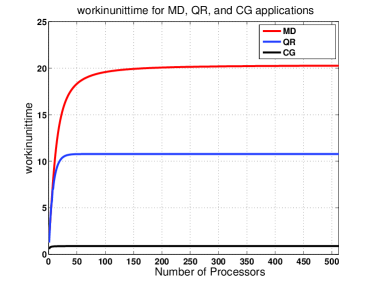
Figure 4: $workininuttime$ values for the applications

TABLE I: Checkpointing ($C$) and Recovery ($R$) Overheads

	$C$ (secs.)			$R$ (secs.)
Application	Min	Avg	Max	Min	Avg	Max
QR	91.90	99.19	117.28	8.74	17.21	32.97
CG	8.96	9.55	9.75	8.89	12.56	15.12
MD	1.35	1.84	2.70	8.27	14.12	17.05

VI-C Evaluation

For an application with a given $workinunittime$, $C$, $R$, and $rp$, our models were invoked for different execution segments for the failure traces of a system. A given execution segment for a failure trace on a system of $N$ processors, corresponds to a random start time, $start$, and random duration, $dur$, for application execution. Based on $start$, $\lambda$ and $\theta$ are calculated for the execution segment using the history of failures that occurred on the processors before $start$. Our model, $M^{mall}$, is invoked with the parameters, $workinunittime$, $C$, $R$, $rp$, $N$, $\lambda$ and $\theta$ for a given application, and execution segment for a failure trace of a system, with different values of $I$.

We have developed a simulator to assess the quality of the checkpointing intervals determined by our model for an application execution on an execution segment. Our simulator uses the same inputs to our model along with duration, $dur$, for simulating the application execution that started at $start$ point in the failure trace and executed for $dur$ seconds. At $start$, the simulator considers the number of available processors and based on the rescheduling policy, $rp$, chooses a set of available processors, $a_{1}$, for application simulation. The simulator then simulates application execution by advancing the time and accumulating checkpointing intervals, $I$ to the useful computation time, $u_{a_{1}}$. After every $I$ seconds, the simulator simulates application checkpointing by advancing $C_{a_{1}}$ seconds in time. This is repeated until a failure occurs in one of the $a_{1}$ processors. At this point, the simulator calculates the amount of useful work spent on $a_{1}$ processors, $uw_{a_{1}}$ as $uw_{a_{1}}=workinunittime_{a_{1}}\times u_{a_{1}}$. It accumulates $uw_{a_{1}}$ to total amount of useful work, $UW$. After failure, the simulator once again considers the number of available processors. If none of the processors are available, the simulator adds the time corresponding to waiting for one of the processors to be repaired for application continuation. At that point in time, the simulator considers the total number of available processors, and based on the rescheduling policy, $rp$, chooses another set of available processors, $a_{2}$, for application execution. Based on the previous and current set of processors for application execution, $a_{1}$ and $a_{2}$, respectively, the simulator advances the time by $R_{a_{1},a_{2}}$ seconds for recovery. After recovery, the simulator once again advances time by accumulating checkpointing intervals, $I$, until one of the processors in $a_{2}$ fails at which point it calculates the useful work spent in $a_{2}$ processors, $uw_{a_{2}}$, and adds this to total useful time, $UW$. This process continues until the simulator reaches $start+dur$ seconds of time, at which point it outputs the total useful work performed by the application as $UW$.

For a given application execution in an execution segment of a failure trace, we calculate model efficiency. To find model efficiency, we find the checkpointing interval, $I_{model}$, corresponding to large $UWT_{model}$ values produced by the model. We then find the useful work output by the simulator, $UW_{I_{model}}$, for the execution segment corresponding to $I_{model}$. We also find the highest useful work, $UW_{highest}$, output by the simulator for the execution segment when executed with different values of checkpointing interval. We denote the checkpointing interval corresponding to $UW_{highest}$ as $I_{sim}$. We find the percentage difference, $pd$, between $UW_{highest}$ and $UW_{I_{model}}$ to give the percentage of work lost due to executing the application with the interval determined by our model. The percentage difference, $pd$, represents the model inefficiency, while $(100-pd)$ represents the model efficiency.

Due to modeling errors, instead of choosing the interval corresponding to the highest $UWT_{model}$ value, we choose the intervals corresponding to $UWT_{model}$ values that are within 8% of the highest $UWT_{model}$. We then calculate the average of these intervals as $I_{model}$. For exploring different checkpoint intervals to determine $I_{model}$, we use a minimum checkpoint interval, $I_{min}$. The checkpointing intervals are doubled starting from $I_{min}$ until the $UWT_{model}$ for the current checkpoint interval is less than the value for the previous interval. We then perform binary-search within the intervals corresponding to the top three $UWT_{model}$ values to explore more checkpointing intervals corresponding to high $UWT_{model}$ values. For this work, we use 5 minutes for $I_{min}$.

VI-D Results

Table II shows the model efficiency for different number of processors on different systems for QR application with greedy rescheduling policy. In all cases, the efficiency of our model in terms of the amount of useful work performed by the application in the presence of failures, using the intervals determined by our model, as shown in column 5, was greater than 80%. Thus, the intervals determined using our models are highly efficient for executing malleable parallel applications on systems with failures. We also find that the checkpointing intervals determined by our model increases with decrease in failure rates of systems indicating that the model presents practically relevant checkpointing intervals. The average $UWT$ values, determined using the simulator, corresponding to $I_{model}$ and $I_{sim}$ are comparable and follow similar trends for the different systems. This shows that the checkpointing intervals determined by our models are highly competent with the best checkpointing intervals. The intervals determined by our model are smaller for the Condor systems than for the batch systems, with the interval approximately equal to 35 minutes when considering execution of malleable parallel applications on a Condor pool of 256 processors. This is due to the highly volatile non-dedicated Condor environment as indicated by the higher failure rates or $\lambda$s for the Condor systems. However, we find that our model efficiencies for the Condor systems are equivalent to the efficiencies for the batch systems, implying that our model can determine efficient checkpointing intervals for both dedicated batch systems and non-dedicated interactive systems.

TABLE II: Model Efficiencies for Different Systems (QR application, greedy rescheduling policy)

Procs.	System	Average $\lambda$	Average $\theta$	Average Model Efficiency %	Average $I_{model}$ (hours)	Average $UWT$ for $I_{model}$	Average $UWT$ for $I_{sim}$
64	system-1	1/(6.42 days)	1/(47.13 min.)	80.17	2.81	8.27	9.45
128	system-1	1/(104.61 days)	1/ (56.03 min.)	90.37	17.78	9.57	10.46
256	system-2	1/(81.82 days)	1/(168.48 min.)	86. 14	5.32	8.67	9.85
512	system-2	1/(68.36 days)	1/(115.43 min.)	95.74	3.68	9.76	10.17
64	condor	1/(6.32 days)	1/(52.377 min.)	82.33	2.75	8.44	9.52
128	condor	1/(6.36 days)	1/(54.848 min.)	87.19	1.53	8.26	9.08
256	condor	1/(5.19 days)	1/(125.23 min.)	93.38	0.67	7.89	8.32

We also compared the model efficiencies for the three applications on 128 processors of system-1 with greedy rescheduling strategy. Table III shows the efficiencies for the applications. The table shows that the checkpointing intervals by our models are more than 90% efficient in terms of the amount of useful work performed by the applications. This shows that our modeling strategy is applicable to different applications. We find that the checkpointing intervals determined by our model, $Imodel$, are largest for the QR application. As shown in Table I, QR application has high checkpointing and recovery overheads. Hence our modeling strategy tries to maximize the amount of useful work for the QR application by selecting larger checkpointing intervals resulting in smaller non-useful or down times for the application. We find that the $UWT$ values corresponding to $I_{model}$ and $I_{sim}$ are comparable. For all the three applications, the $UWT$ values calculated for application executions in the presence of failures are within 4-11% of the corresponding failure-free maximum $workinunittime$ values shown in Figure 4. This shows that by adopting malleability, and choosing efficient checkpointing intervals by our models, applications can execute with nearly failure-free high performance even in the presence of failures.

TABLE III: Model Efficiencies for the 3 Applications (system-1, 128 processors, greedy rescheduling policy)

Application	Average Model Efficiency %	Average $I_{model}$ (hours)	Average $UWT$ for $I_{model}$	Average $UWT$ for $I_{sim}$
QR	90.37	17.78	9.57	10.47
CG	95.66	7.59	0.85	0.88
MD	90.06	13.7	17.96	19.72

We also investigated the usefulness of non-dedicated highly-volatile Condor environments for the execution of malleable parallel applications. The work by Plank and Thomason[10] showed that Condor systems, due to high failure rates and checkpointing overheads, are not suitable for execution of moldable applications since a fixed number of processors are generally not available for the entire duration of application execution on such systems. Accordingly, it was shown that execution on only one processor in Condor environment provided the least runtimes for the applications. We explored the use of such systems for malleable applications. Figure 5 shows simulation of a sample execution of QR application on 128 processors of the Condor system for a duration of 80 days with the greedy rescheduling policy. $I_{model}$ of 1.53 hours, the checkpointing interval determined by our model, was used for the execution. We also used $C=R=20$ minutes, the worst-case checkpointing and recovery overheads on shared Condor systems and networks.

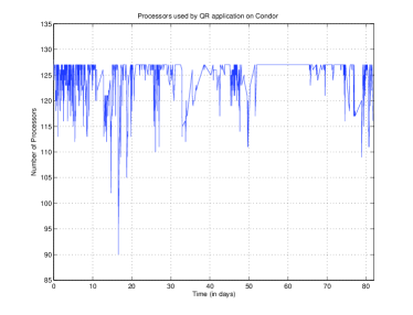
Figure 5: Simulation of QR application execution on Condor system for 80 days (128 processors, checkpointing interval = $I_{model}$ = 1.53 hours, $C=R=$ 20 minutes)

As Figure 5 shows, different number of processors are used for execution at different times. More than 100 processors are used in most cases since the greedy rescheduling strategy chooses the maximum number of processors available for execution. The $UWT$ value for this execution is 7.29. This $UWT$ value, obtained in the presence of failures on the Condor systems, is nearly 70% of the corresponding failure-free maximum $workinunittime$ value for QR application shown in Figure 4. Thus, while highly volatile environments like Condor are not suitable for executions of moldable applications, they can be used to provide high efficiency for malleable applications due to the flexibility in terms of the number of processors used for execution and the efficient checkpointing intervals determined by our models.

Table IV shows the model efficiency and the amount of useful work corresponding to the intervals determined by our models for the three rescheduling policies for QR application on 128 processors of system-1. We find that in all the rescheduling policies, the efficiency was greater than 80%. We also find that the AB rescheduling policy yields the maximum work for the application. This is because the policy attempts to execute the application on small number of processors where the mean time to failures is low. Hence larger checkpointing intervals are chosen for application execution, as shown in the table, leading to less checkpointing overheads and more useful work. The greedy strategy performs the least useful work since it always executes the application on maximum number of available processors where the mean time to failures is high leading to high checkpointing and recovery overheads. The PB policy considers number of processors for which failure-free running time is minimum. Since the QR application is highly scalable, the PB rescheduling policy attempts to execute on large number of processors where the failure rates are high. Hence, the checkpointing intervals and the resulting amount of useful work for the PB policy are comparable to those for the greedy policy. Thus, we find that for large number of systems with failures, executing on smaller number of systems with less failure rates (AB) leads to more useful work by the application than executing the application on the number of processors corresponding to maximum performance (PB).

TABLE IV: Model Efficiencies for Different Rescheduling Policies (QR application, system-1, 128 processors)

Resched. Policy	Average Model Efficiency %	Average $I_{model}$ (hours)	Average $UW_{I_{model}}$ $(\times 10^{6})$
Greedy	90.3	17.41	108.27
PB	90.0	17.44	110.20
AB	83.1	88.42	133.15

Figure 6(a) shows the model inefficiencies with increasing failure rates for QR application on a condor trace with 256 processors and for greedy rescheduling policy. The figure shows that the model inefficiencies decrease or model efficiencies increase with increasing failure rates. Thus our model is effectively able to predict application behavior on systems with frequent failures than for systems with sporadic failures. This is because the history of failure rates on systems with sporadic failures cannot be effectively used to predict the future failures on those systems. We also compared the model efficiencies for varying durations of application execution. Figure 6(b) shows the results for QR application execution with condor traces on 128 processors and for greedy rescheduling policy. The results show that our model inefficiency decreases or model efficiency improves with increasing durations. This is because the long-running properties of our Markov model are especially suited for long-running parallel applications than for short applications.

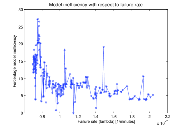
(a) Different Failure Rates (256 processors)

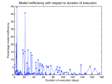
(b) Different Durations (128 processors)

Figure 6: Model Efficiency for Different Failure Rates and Durations (QR application, condor trace, greedy rescheduling policy)

VI-E Summary

In addition to showing validation and efficiency results, our experiments have also shown some interesting and new observations. We have shown that with the help of malleability and our checkpointing intervals, applications can execute with near failure-free performance in the presence of failures. We have also shown that malleability and our checkpointing intervals encourage executions on volatile environments like Condor, the environments considered to be not suitable for parallel applications in the earlier efforts.

VII Related Work

There is a vast amount of literature on checkpointing interval selction[9]. In this section, we focus on some of the highly relevant efforts. The work by Daly[16] develops a first-order model to determinine optimum checkpointing interval. The work then develops a higher-order model for improving accuracy for small talues of MTBF. The work assumes Poisson failure rate and considers single processor failures.

The work by Nurmi et al.[17] determines checkpointing intervals that maximize efficiency of an application when executed on volatile resource-harvesting systems such as Condor[12] and SETI@Home[18]. They use three different distributions including exponential, Weibull and hyper-exponential for fitting hostorical data on machine availabilty. They then use the future lifetime distribution along with the checkpoint parameters including checkpointing intervals in a three-state Markov model for application execution and determine the interval that minimize execution time. Their Markov model is based on the work by by Vaidya[19]. Their work is intended for sequential processes executing in the Condor environment. They show that the type of failure distribution does not affect the application execution performance.

The work by Ren et al.[20] considers proving fault tolerance for guest jobs executing on resources provided voluntarily in fine grained cycle sharing (FGCS) systems. In their work, they calculate checkpointing interval using a low overhead one-step look ahead heuristic. In this heuristic, they divide execution time into steps and compare the costs of checkpointing at a step and the subsequent step using the probability distribution function for failures. Their model does not assume a specific distribution and is intended for sequential guest jobs.

Plank and Elwasif[21] study the implications of theoretical results related to optimal checkppointing intervals on actual performance of application executions in the presence of failures. They perform the study using simulations of long running applications with failure traces obtained on three parallel systems. One of the primary results of their work is that the exponential distribution of machine availability, although inaccurate, can be used for practical purposes to determine checkpointing intervals for parallel applications.

To our knowledge, the model by Plank and Thomason[10] is the most comprehensive model for determining checkpointing intervals for parallel applications. Their work tries to determine the number of processors and checkpointing interval for executing moldable parallel applications on a parallel system given a failure trace on the system. The model assumes exponential distribution for inter-arrival times of failures. They use the concept of spare processors for replacing the systems that failed during application execution. They show by means of simulations that checkpointing intervals determined by their model lead to reduced execution times in the presence of failures. Their work was intended for typical parallel checkpointing systems that do not allow the number of processors to change during application execution. With increasing prevelance of checkpointing systems for malleable parallel applications, we base our work on their model and significantly modify different aspects of their model to determine checkpointing intervals for such systems.

VIII Conclusions

The work described in this paper presents the first effort, to our knowledge, for selecting checkpointing intervals for efficient execution of malleable parallel applications in the presence of failures. The work is based on a Markov model for malleable applications that includes states for execution on different number of processors during application execution. We have also defined a new metric for evaluation of such models. The states of our model are based on rescheduling policies. By conducting large number of simulations with failure traces obtained for real high performance systems, we showed that the checkpointing intervals determined by our model lead to efficient executions of malleable parallel applications in the presence of failures.

IX Future Work

We plan to augment our model with different kinds of failure distributions. We also plan to experiment with different redistribution policies. The checkpoint intervals from our model will be integrated with a real checkpointing system that provides malleability and fault tolerance. Finally, we plan to extend our model for determining checkpointing intervals for executions on multi-cluster grids and heterogeneous systems.

References

- [1] http://www.top500.org.
- [2] L. Oliker, A. Canning, J. Carter, C. lancu, M. Lijewski, S. Kamil, J. Shalf, H. Shan, E. Strohmaier, S. Ethier, and T. Goodale, “Scientific Application Performance on Candidate PetaScale Platforms,” in IPDPS ’07: Proceedings of the 21st IEEE International Parallel and Distributed Processing Symposium, 2007, pp. 1–12.
- [3] F. Petrini, K. Davis, and J. Sancho, “System-Level Fault-Tolerance in Large-Scale Parallel Machines with Buffered Coscheduling,” in IPDPS ’04: Proceedings of the 21st IEEE International Parallel and Distributed Processing Symposium, 2004, pp. 209–.
- [4] L. Chen, Q. Zhu, and G. Agrawal, “Supporting Dynamic Migration in Tightly Coupled Grid Applications,” in SC ’06: Proceedings of the 2006 ACM/IEEE conference on Supercomputing, 2006, p. 117.
- [5] J. Ruscio, M. Heffner, and S. Varadarajan, “DejaVu: Transparent User-Level Checkpointing, Migration, and Recovery for Distributed Systems,” in IPDPS ’07: Proceedings of the 21st IEEE International Parallel and Distributed Processing Symposium, 2007, pp. 1–8.
- [6] R. Fernandes, K. Pingali, and P. Stodghill, “Mobile MPI Programs in Computational Grids,” in PPoPP ’06: Proceedings of the eleventh ACM SIGPLAN symposium on Principles and Practice of Parallel Programming, 2006, pp. 22–31.
- [7] M. Schulz, G. Bronevetsky, R. Fernandes, D. Marques, K. Pingali, and P. Stodghill, “Implementation and Evaluation of a Scalable Application-Level Checkpoint-Recovery Scheme for MPI Programs,” in Supercomputing, 2004. Proceedings of the ACM/IEEE SC2004 Conference, 2004, pp. 38–.
- [8] S. Vadhiyar and J. Dongarra, “SRS - A Framework for Developing Malleable and MigratableParallel Applications for Distributed Systems,” Parallel Processing Letters, vol. 13, no. 2, pp. 291–312, 2003.
- [9] E. Elnozahy, D. Johnson, and Y. Wang, “A Survey of Rollback-Recovery Protocols in Message-Passing Systems,” Dept. of Computer Science, Carnegie Mellon University, Tech. Rep. CMU-CS-96-18, 1996.
- [10] J. Plank and M. Thomason, “Processor Allocation and Checkpoint Interval Selection in Cluster Computing Systems,” Journal of Parallel and Distributed Computing, vol. 61, no. 11, pp. 1570–1590, 2001.
- [11] http://institute.lanl.gov/data/lanldata.shtml.
- [12] http://www.cs.wisc.edu/condor.
- [13] L. S. Blackford, J. Choi, A. Cleary, E. D’Azevedo, J. Demmel, I. Dhillon, J. Dongarra, S. Hammarling, G. Henry, A. Petitet, K. Stanley, D. Walker, and R. C. Whaley, ScaLAPACK Users’ Guide. Society for Industrial and Applied Mathematics, Philadelphia, PA, 1997.
- [14] S. Balay, K. Buschelman, W. Gropp, D. Kaushik, M. Knepley, L. McInnes, B. Smith, and H. Zhang, “PETSc Web Page,” 2001, http://www.mcs.anl.gov/petsc.
- [15] http://zeus.df.ufcg.edu.br/labfit.
- [16] J. Daly, “A Higher Order Estimate of the Optimum Checkpoint Interval for Restart Dumps,” Future Generation Computer Systems, vol. 22, no. 3, pp. 303–312, 2006.
- [17] D. Nurmi, R. Wolski, and J. Brevik, “Model-based checkpoint scheduling for volatile resource environments,” Dept. of Computer Science, University of California Santa Barbara, Tech. Rep. 2004-25, 2004.
- [18] http://setiathome.ssl.berkeley.edu.
- [19] N. Vaidya, “Impact of Checkpoint Latency on Overhead Ratio of a Checkpointing Scheme,” IEEE Transactions on Computers, vol. 46, no. 8, pp. 942–947, 1997.
- [20] X. Ren, R. Eigenmann, and S. Bagchi, “Failure-Aware Checkpointing in Fine-Grained Cycle Sharing Systems,” in HPDC ’07: Proceedings of the 16th International Symposium on High Performance Distributed Computing, 2007, pp. 33–42.
- [21] J. Plank and W. Elwasif, “Experimental Assessment of Workstation Failures and Their Impact on Checkpointing Systems,” in FTCS ’98: Proceedings of the The Twenty-Eighth Annual International Symposium on Fault-Tolerant Computing, 1998, p. 48.