Spectroscopic properties of
a two-dimensional time-dependent Cepheid model
II. Determination of stellar parameters and abundances

Abstract

Context. Standard spectroscopic analyses of variable stars are based on hydrostatic 1D model atmospheres. This quasi-static approach has not been theoretically validated.

Aims. We aim at investigating the validity of the quasi-static approximation for Cepheid variables. We focus on the spectroscopic determination of the effective temperature $T_{\mathrm{eff}}$, surface gravity $\log\,g$, microturbulent velocity $\xi_{\mathrm{t}}$, and a generic metal abundance $\log\,A,$ here taken as iron.

Methods. We calculated a grid of 1D hydrostatic plane-parallel models covering the ranges in effective temperature and gravity that are encountered during the evolution of a 2D time-dependent envelope model of a Cepheid computed with the radiation-hydrodynamics code CO5BOLD. We performed 1D spectral syntheses for artificial iron lines in local thermodynamic equilibrium by varying the microturbulent velocity and abundance. We fit the resulting equivalent widths to corresponding values obtained from our dynamical model for 150 instances in time, covering six pulsational cycles. In addition, we considered 99 instances during the initial non-pulsating stage of the temporal evolution of the 2D model. In the most general case, we treated $T_{\mathrm{eff}}$, $\log\,g$, $\xi_{\mathrm{t}}$, and $\log\,A$ as free parameters, and in two more limited cases, we fixed $T_{\mathrm{eff}}$ and $\log\,g$ by independent constraints. We argue analytically that our approach of fitting equivalent widths is closely related to current standard procedures focusing on line-by-line abundances.

Results. For the four-parametric case, the stellar parameters are typically underestimated and exhibit a bias in the iron abundance of $\approx-0.2\,\mbox{dex}$. To avoid biases of this type, it is favorable to restrict the spectroscopic analysis to photometric phases $\phi_{\mathrm{ph}}\approx 0.3\ldots 0.65$ using additional information to fix the effective temperature and surface gravity.

Conclusions. Hydrostatic 1D model atmospheres can provide unbiased estimates of stellar parameters and abundances of Cepheid variables for particular phases of their pulsations. We identified convective inhomogeneities as the main driver behind potential biases. To obtain a complete view on the effects when determining stellar parameters with 1D models, multidimensional Cepheid atmosphere models are necessary for variables of longer period than investigated here.

1 Introduction

Cepheids are some of the most important variable stars in observational astronomy. First, the Cepheid period-luminosity (PL) relation (Leavitt, 1908; Leavitt & Pickering, 1912) is a powerful astrophysical tool to measure distances within the Galaxy, and to measure cosmological scales (Riess et al., 2016). However, the chemical composition affects Cepheid pulsational properties, and it also reflects on the associated extragalactic distance scale, even if no general consensus exists in the literature on the size and the sign of the effect. The accurate spectroscopic analysis of Romaniello et al. (2005, 2008) shows that the metallicity affects the V-band Cepheid PL relation and that metal-rich Cepheids appear to be systematically fainter than metal-poor ones at a fixed period, in agreement with theoretical prescriptions (Bono et al., 1999; Marconi et al., 2005).

Second, Cepheids are most convenient for a detailed study of radial abundance gradients across the Galactic disk: abundances have been derived for up to 25 elements from C to Gd (Andrievsky et al., 2002b; Lemasle et al., 2013; Genovali et al., 2015; da Silva et al., 2016). Because they are bright supergiants, they allow us to probe the inner disk (Genovali et al., 2013; Martin et al., 2015; Andrievsky et al., 2016) as well as the outermost regions (Andrievsky et al., 2004; Lemasle et al., 2008; Luck et al., 2011).

Standard abundance determinations for Cepheids and non-pulsating stars are based on grids of 1D hydrostatic stellar atmospheres. Calculations of multidimensional Cepheid models are a sizable computational problem because of the different spatial and temporal scales.

During pulsations, the thermal structure of a Cepheid atmosphere changes. The effective temperature, gravity, and microturbulent velocity depend on the pulsation phase (Andrievsky et al., 2002b, c; Luck et al., 2003; Andrievsky et al., 2004), but the metallicity does not (nor do individual abundances). Standard grids of 1D hydrostatic models cover the necessary wide range of stellar parameters (Kurucz, 1992; Gustafsson et al., 2008), typically adopting the mixing-length theory (MLT, see Böhm-Vitense 1958) to describe convection. Gautschy (1987) argued that for a Cepheid with a 10-day pulsational period, deviations from hydrostatic conditions should be on a level of a few percent. However, the thermal structure, which sets the conditions for the line formation, differs from the corresponding thermal structure obtained in hydrostatic models because of strong disturbances. Hence, the correctness of the standard approach for determining stellar parameters and abundances has to be validated.

In a previous paper (Vasilyev et al. 2017, hereafter Paper I), we have introduced a 2D time-dependent Cepheid model calculated with the radiation-hydrodynamics code CO5BOLD (Freytag et al., 2012).

Here, we consider results of spectral syntheses taking the 2D Cepheid model to provide artificial observational data, and apply the standard approach to determine stellar parameters using 1D plane-parallel hydrostatic model atmospheres. Stellar parameters are exactly known for the 2D model. Thus, we can check the standard approach for biases on parameters, including dependencies on the pulsational phase. Since we only have one multidimensional model at hand, our findings are restricted to the class of short-periodic Cepheids.

The paper is organized as follows. Basic properties of the 2D Cepheid model are summarized in Sect. 2. The grid of 1D models is presented in Sect. 3. In Sect. 4 we describe the line list and compare it with line lists that are applied in measuring Galactic metallicity gradients. Features of spectral line profiles from the 2D model are discussed in Sect. 5. Results for the determination of stellar parameters for the four-, three- and two-parameter case are presented in Sect. 7.

2 Two-dimensional Cepheid model

Radiation-hydrodynamics simulations of a short-periodic 2D Cepheid model in Cartesian geometry employing gray radiative transfer were calculated with the CO5BOLD code (Freytag et al., 2012). The model has a nominal effective temperature of $T_{\mathrm{eff}}=5600$ K, a constant depth-independent gravitational acceleration of $\log\,g=2.0$, and solar metallicity. The model shows self-excited pulsations presumably due to the $\kappa$-mechanism (Eddington, 1917; Zhevakin, 1963) in the fundamental mode with a pulsational period of $\approx 2.8$ days. The model features are a realistic treatment of convection and radiative transfer. The construction of the model was a numerical challenge because of the extremely small time step imposed by the short radiative relaxation time in the employed time-explicit numerical scheme. It enforces the restriction to 2D models, at the moment. A detailed description of the physical and spectroscopic properties of the model, including the effects of the Cartesian geometry and gray radiative transfer, can be found in Paper I.

Starting with the initial hydrostatic condition, the 2D model reaches a quasi-stationary state with developed convection at $t\approx 4.5\times 10^{6}$ s (see Fig. 2 in Paper I). Furthermore, the model exhibits self-excited oscillations starting at $t\approx 6\times 10^{6}$ s. Ninety-nine 2D snapshots between these instances in time were taken for the analysis of the hydrostatic non-pulsating regime. For the analysis of the pulsating regime, radiation hydrodynamics simulations provided 150 2D snapshots covering six full pulsation periods.

3 Grid of 1D LHD models

A grid of 1D plane-parallel hydrostatic models was calculated using a Lagrangian hydrodynamics code (here after LHD), which solves the set of 1D radiation-hydrodynamics equations in the Lagrangian frame. Convective fluxes and velocities were calculated according to MLT. In the present work, the mixing-length parameter $\alpha$ was fixed to 1.5 for all 1D models. The actual value of the mixing-length parameter has a minor effect on the photospheric temperature structure of the 1D models since the the convective zone does not reach into the optically thin regions of the giant stars considered here.

The radiative flux of 1D LHD models was calculated using gray opacities. The radiative transfer equation was solved adopting the Feautrier scheme (Feautrier, 1964). Opacities, the equation of state, and the chemical composition were taken as for the 2D model. The effective temperatures of 1D models were varied between 4900 K and 6000 K in steps of $\Delta T=100$ K. They cover the effective temperature range that is encountered during the temporal evolution of the 2D model. The upper boundary of 1D models of the grid was set to below $\log\tau_{\mathrm{R}}<-6$ to contain the line-formation regions of the given line list, which is described in the next sections.

The surface gravity $\log\,g$ of 1D LHD models was taken in the range 0.7 to 3.5 in steps of $\Delta\log\,g=0.2$ to cover the effective gravity range – including acceleration effects – found in the 2D model. The equivalent width (EW) of a spectral line depends on the physical conditions in the line formation region of the stellar atmosphere. The pressure is one of the key quantities that influence the EW. This quantity, in turn, is controlled by the surface gravity $\@vec{g}$. In stellar atmospheres that are in hydrostatic equilibrium, the pressure gradient, $\nabla p$, is balanced by the gravity force:

$$\frac{\@vec{\nabla}p}{\rho}=\@vec{g},$$ (1)

where $\rho$ is the density. In the 2D model, the dynamics adds to the purely gravitational acceleration, which results in a total acceleration that has to be balanced by the pressure gradient. The effective gravitational acceleration is the sum of the effects of gravity and kinematic acceleration, $\frac{d\@vec{v}}{dt}$:

$$\frac{\@vec{\nabla}p}{\rho}=\@vec{g}-\frac{d\@vec{v}}{dt}=\@vec{g_{\mathrm{\,eff}}}.$$ (2)

In the 2D model, the gas and turbulent pressures $\@vec{\nabla}p=\@vec{\nabla}p_{\mathrm{gas}}+\@vec{\nabla}p_{\mathrm{t}}$ contribute to the total pressure. Since it is primarily caused by convection, the turbulent pressure $p_{\mathrm{t}}$ is significant at the bottom of the photosphere. However, the gas pressure gradient still provides the dominant contribution to the total pressure gradient even deep in the photosphere (see Fig. 5 in Paper I) and line-formation regions. Finally, the effective gravity of the 2D model was derived with the total pressure gradient. We did not include turbulent pressure in the 1D models so that $\nabla p=\nabla p_{\mathrm{gas}}$. Even if we had tried to do so in the framework of MLT, it would have had little effect since the convective zone is restricted to layers below the photosphere.

If we consider a Lagrangian mass shell following the mean vertical mass motion in the line formation region, we find that it is subject to substantial acceleration during the pulsations. When the direction of motion at the phase of maximum compression is reversed, it experiences an acceleration of $\approx(1.0\ldots 2.5)\,\@vec{g}$. In total, this corresponds to an effective gravitational acceleration of $\@vec{g_{\mathrm{\,eff}}}\approx(2.0\ldots 3.5)\,\@vec{g}$, which in 1D models would have to be balanced by the pressure gradient according to Eq. (2). For now, we recall that the line formation in a dynamical atmosphere occurs under a variable effective gravity. While kinematic effects have a rather obvious impact, spectroscopically determined surface gravities can also be affected for other reasons. For instance, according to Steffen (1985) and Korn et al. (2003), the surface gravity of Procyon as deduced from the ionization balance is inconsistent with an independent estimate obtained with astrometric methods.

For Cepheids, a mean gravity can be estimated without a spectroscopic analysis. Gough et al. (1965) theoretically derived the ”period-gravity” relation,

$$P\sim g^{-1},$$ (3)

where $P$ is the pulsational period. The empirically calibrated ”period-gravity” relation of Tsvetkov (1988) can be used to estimate the mean gravity, and this can be taken as a first approximation to derive stellar parameters. According to Andrievsky et al. (2002b) (their Fig. 1), however, pulsations produce a scatter of 0.8 around the mean value.

The full grid of 1D LHD models in the $T_{\mathrm{eff}}$–$\log\,g$ plane is shown in Fig. 1. With different temperature and gravity grid models, we intend to represent the states of the dynamical 2D atmosphere encountered in the different pulsational phases. It is clear that hydrostatic equilibrium is never exactly reached in the 2D model. The timescale to attain hydrostatic equilibrium is on the order of the sound-crossing time, which is on the same order as the pulsational period. We might expect conditions with low effective gravity around the phase of maximum expansion. At this point, the timescale of the convective instability becomes longer than the pulsational period because of a low effective gravity, which in turn decreases the efficiency with which the turbulence is generated. The thermal structure is less perturbed by dynamical effects than in the phase of maximum compression. For et al. (2011) found that photometric phases around $\approx 0.35$ (photometric phase zero corresponds to maximum light) are optimal for chemical abundance analyses of RR Lyrae stars with hydrostatic model atmospheres. Recalling the differences between RR Lyrae and Cepheid variables (RR Lyr stars have higher effective temperatures, higher velocity amplitudes, shorter periods of pulsation, and exhibit stronger atmospheric shocks), we expect similarities and address this point below.

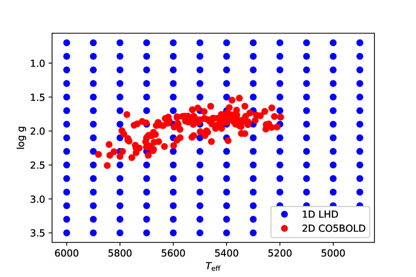
Figure 1: Grid of 1D hydrostatic LHD models (blue circles) in the $T_{\mathrm{eff}}$–$\log\,g$ plane, and effective temperatures and gravities of the 2D model (red circles) for 150 instances in time, covering six full periods of pulsation.

4 List of artificial iron lines

For an accurate spectroscopic analysis, the line list and wavelength interval have to be carefully selected. Classically, the line list for the metallicity determination contains isolated, unblended iron lines of different ionization stages and excitation energies that cover a wide range of EWs. The line strength depends on the physical conditions in the stellar atmosphere. Thus, depending on the star, we have to include or exclude different spectral lines in the analysis.

To keep our analysis general and to obtain a systematic overview, we did not use a particular list of Fe i and Fe ii lines. Instead, our line list consisted of 49 fictitious neutral and singly-ionized iron lines with a fixed wavelength of $\lambda=5000$ Å. Excitation energies of the Fe i and Fe ii lines were taken to be $E_{\mathrm{i}}^{{Fe\textsc{i}}}=1,3,5$ eV and $E_{\mathrm{i}}^{{Fe\textsc{ii}}}=1,3,5,10$ eV, respectively. The oscillator strengths were set to cover a wide range of EWs from 5 mÅ to 200 mÅ.

Figure 2 shows the line parameters in the excitation potential – oscillator strength plane. We also plot a list of real Fe i and Fe ii lines, which was used by Lemasle et al. (2007, 2008), Pedicelli et al. (2010), and Genovali et al. (2013, 2014), to investigate the chemical composition of Galactic Cepheids and measure the Cepheid metallicity gradient in different parts of the Galactic disk. The group of Fe ii 10 eV lines is unrealistic with respect to lines used in observational analyses because of large oscillator strengths and excitation potential. Owing to the high-excitation energy, these lines form in deep regions of the atmosphere. As a consequence, they are strongly influenced by convection. Especially during the maximum compression phase, the convection is amplified through the high effective gravity (see Paper I). In order to be closer to the list of real lines, and because of the strong sensitivity of the Fe ii 10 eV lines to dynamical effects, we did not consider these lines when we determined the stellar parameters of the dynamical model. On the other hand, because of the infinite signal-to-noise ratio of our theoretical spectra, we did not exclude the weakest lines with excitation potentials of 1, 3, and 5 eV in the analysis. The spectral synthesis was performed with Linfor3D (Gallagher et al., 2017) for the dynamical and 1D LHD models assuming local thermodynamic equilibrium.

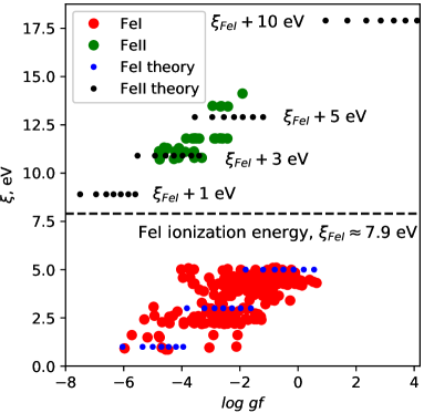
Figure 2: Real (large circles) and our theoretical (small circles) Fe i and Fe ii lines in the excitation energy–oscillator strength plane.

Before we describe our method for determining the stellar parameters and present our results, we first discuss the features of the line profiles of the dynamical model.

5 Spectral line profiles of the dynamical 2D model

The homogeneous expansion or contraction of the atmosphere of a spherical pulsating star transforms a symmetric Gaussian absorption line into a characteristically asymmetric shifted line profile, as was shown early on by Shapley & Nicholson (1919). The asymmetry and shift depend on the radial velocity of the line formation region (Nardetto et al., 2006). However, the expansion or contraction of the atmosphere of a pulsating star is not perfectly homogeneous. This can, for instance, be observed in Balmer line profiles of RR Lyrae stars (Preston, 2011) or is predicted by global 3D radiation-hydrodynamics models of AGB stars (Freytag et al., 2017), and it is also demonstrated by our results in Paper I. While in observations the line profile is observed averaged over the whole stellar disk, the spectral synthesis for our 2D model provides information on the variation in the spectral line profile in a spatially resolved fashion.

Figure 3 shows the spatial variation along the horizontal position in the modeled 2D box of the normalized line profile of the strongest Fe ii 3 eV line in terms of intensity in vertical direction (inclination cosine $\mu=1$). The particular instance in time corresponds to a photometric phase of 0.56, illustrating a situation during the contracting phase of the 2D model. Absorption as well as emission features are discernible. The line profiles vary widely in terms of radial velocities and asymmetry, sometimes showing a multi-component structure. The mean radial velocity is roughly 10 kms^-1 for the given example, with significant spatial variations caused by convective inhomogeneities.

Around a horizontal position $x\approx 7.5\times 10^{11}$ cm, emission lines are present. Figure  4 shows vertical 1D thermal $T(\tau_{\mathrm{R}})$ and radial velocity profiles around the location of emission. We note that we use the spectroscopic sign convention for the radial velocity, where a negative velocity corresponds to a motion toward the observer and vice versa. The Fe ii 3 eV line formation region is located at $\log\tau_{\mathrm{R}}\approx-3\ldots 0.7$. Emission line profiles occur because of an inverse gradient of the temperature at optical depths $\log\tau_{\mathrm{R}}<-1.5$. The photospheric temperature of the thermal profile is $\approx 4000$ K. Local disturbances of the thermal profile by convection can produce cold regions. However, as was shown in Paper I, the variation in effective temperature of the mean 2D model, which is the result of the horizontal averaging of the full 2D model at fixed geometrical height, varies in a range between $5300$ and $5900$ K.

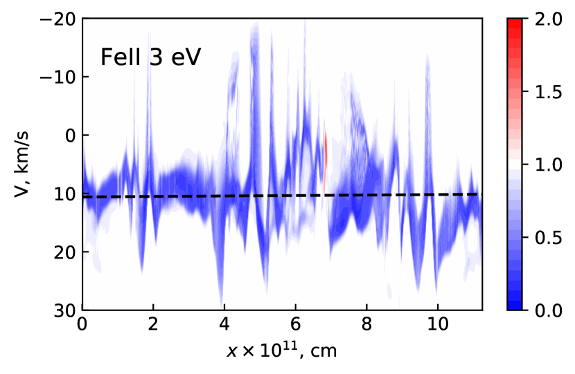
Figure 3: Two-dimensional map of normalized line profiles of the strongest Fe ii 3 eV line in terms of normalized intensity for a photometric phase of $\phi_{\mathrm{ph}}=0.56$. The horizontal axis shows the horizontal spatial position within the modeled box. The vertical axis represents the wavelength expressed as Doppler velocity. Emission and absorption are indicated by red and blue lines, respectively. The continuum level is one, and it is shown in white. The mean Doppler velocity is depicted by the dashed line. The standard deviation of the Doppler shift velocities is 6.1 kms^-1.

The inverse temperature gradient and jump of the radial velocity at $\log\tau_{\mathrm{R}}\approx-2$ in Fig. 4 correspond to an accretion front, where almost free-falling low-density material collides with a quasi-hydrostatically stratified deeper layer. The velocity difference between pre- and post-shock regions is $\approx 10$ kms^-1, which is substantial. As was described in Paper I, we applied an artificial drag force at a number of grid layers close to the top, reducing the velocities by a certain fraction per time interval. The drag force, which dampens waves, leads to a heating of the top of the modeled box. This is visible at the temperature profile in the regions where $\log\tau_{\mathrm{R}}<-3.5$. To minimize the effect of the upper boundary, we considered lines that form at $\log\tau_{\mathrm{R}}>-4$.

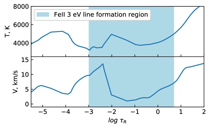
Figure 4: Vertical thermal and radial velocity profiles of the section of the 2D model in which the emission line profile of the strongest fe ii 3 eV line occurs. The line formation region is indicated by the light blue area.

6 Method of the parameter fitting

One of the traditional ways to determine stellar parameters and elemental abundances is based on minimizing the difference between observed and synthesized line profiles by varying the model parameters of a precomputed grid. However, in our analysis, we did not compare line profiles because, as we showed in the previous section, the line profiles of the 2D model are asymmetric, Doppler-shifted, and have a multi-component structure. The line asymmetry depends on the pulsational phase, whereas 1D LHD line profiles are perfectly symmetric and unshifted and thus can only poorly represent the 2D profiles. For these reasons, we only matched the EW of the lines. In the 1D spectral synthesis, the microturbulent velocity $\xi_{\mathrm{t}}$ was varied in the range 0.0 kms^-1 to 7.0 kms^-1 in steps of 0.5 kms^-1 to cover a typical observational range (Andrievsky et al., 2002a). The same microturbulent velocity $\xi_{\mathrm{t}}$ was adopted for all lines from the line list. The result of the spectral synthesis is an array of EWs $W_{\mathrm{i}}=f_{\mathrm{i}}(T_{\mathrm{eff}},\log\,g,\xi_{\mathrm{t}})$, where the index $i$ is a line number running from 1 to 42 for our set of artificial iron lines.

Observationally, the metallicity of an observed star is an unknown parameter. We mimicked this by including the iron abundance (metallicity), $\log\,A$, as an additional parameter together with $T_{\mathrm{eff}}$, $\log\,g$, and $\xi_{\mathrm{t}}$. The EW of a spectral line depends on the product of the abundance $A$ and oscillator strength $gf$, on a logarithmic scale $\log\,A\ +\ \log\,gf$. For a fixed $\log\,gf$, the abundance $\log\,A$ was changed between $-0.6\ldots 0.0$ dex and $0.0\ldots 0.6$ dex in steps of 0.1 dex. Corresponding EWs were calculated using a cubic spline interpolation in $\log\,W$-$\log\,gf$ space.

The EWs calculated with the grid of 1D LHD models were finally used to best match the EWs from the spectral synthesis of the dynamical model. We introduced a $\chi^{2}$ function to characterize the mean relative difference between the EWs of the 2D and 1D models, which is in general a function of the 4D vector $\@vec{p}=\big{\{}T_{\mathrm{eff}},\ \log\,g,\ \xi_{\mathrm{t}},\ \log\,A\big{\}}$

$$\chi^{2}(\@vec{p})=\frac{1}{N}\sum_{j}\Bigg{[}\frac{W^{\mathrm{2D}}_{\mathrm{j}}-W^{\mathrm{1D}}_{\mathrm{j}}(\@vec{p})}{f\cdot\sigma_{\mathrm{Wj}}}\Bigg{]}^{2},$$ (4)

where the sum goes over all iron lines of our line list, $N$ the total number of lines, and $f$ is an arbitrary scaling factor for the assumed uncertainty $\sigma_{\mathrm{w,j}}=W^{\mathrm{2D}}_{j}$. It should be understood that the uncertainty stated above is not a statistical uncertainty, since our synthetic lines are not subject to noise. Taking the uncertainty as proportional to the line strength itself was a convenient and reasonable way to express the deviations in line strengths. We used a scaling factor $f=1,$ which in the following allows a straightforward interpretation of a $\chi^{2}$ value: the square-root of a given $\chi^{2}$ is the relative RMS deviation between 2D model and 1D model line strengths.

The best-fit combination of the parameters is found at the minimum of the $\chi^{2}$ function. We performed an exhaustive search of the minimum over our grid of 1D models and took the model with minimum deviation as a first approximation. To improve the location of the minimum, we interpolated between grid points. We tested three different interpolation methods to further locate the minimum in the 4D parameter space:

1. Radial basis functions (RBF) with a norm

   $$\frac{1}{\sqrt{(\@vec{p}/\Delta\@vec{p})^{2}+1}}=\Big{[}\sum_{i=1}^{4}\Big{(}\frac{p_{\mathrm{i}}}{\Delta p_{\mathrm{i}}}\Big{)}^{2}+1\Big{]}^{-1/2},$$ (5)

   where $\Delta\@vec{p}=\big{\{}\Delta T_{\mathrm{eff}},\Delta\log\,g,\xi_{\mathrm{t}},\Delta\log\,A\big{\}}$ is the smoothing scale. The choice of the scale is based on the spacings in our grid of 1D models, which are $\Delta T_{\mathrm{eff}}=100$ K, $\Delta\log\,g=0.2$ dex, $\xi_{\mathrm{t}}=0.5$ kms^-1, and $\Delta\log\,A=0.1$ dex.

2. A fit of a quadratic form to reconstruct the shape of the function around the minimum.

3. A sequence of 1D cubic piecewise interpolations.

Before we applied the methods for the analysis of EWs of the 2D model, they were tested on EWs of one custom computed 1D model with $T_{\mathrm{eff}}=5550$ K, $\log\,g=2.0$ dex, $\xi_{\mathrm{t}}=1.75$ kms^-1, and $\log\,A=-0.05$ dex, which is located between points of the grid.

6.1 Test with radial basis functions

The minimum point and its 80 nearest-neighbor points were taken to describe the $\chi^{2}$ function with RBFs:

$$\chi^{2}(\@vec{p})=\sum_{j=1}^{81}\frac{\omega_{j}}{\sqrt{\sum_{i=1}^{4}\Big{(}\frac{p_{\mathrm{i}}-p_{\mathrm{ij}}}{\Delta p_{\mathrm{i}}}\Big{)}^{2}+1}},$$ (6)

where the weights $\omega_{\mathrm{j}}$ are results of the solution of the linear system of equations:

$$\sum_{j=1}^{81}p_{\mathrm{ij}}\omega_{\mathrm{j}}=\chi^{2}(\@vec{p}_{\mathrm{i}}),$$ (7)

with $p_{\mathrm{ij}}$ being the distance between the vectors $\@vec{p}_{\mathrm{i}}$ and $\@vec{p}_{\mathrm{j}}$ in the parameter space. The reconstructed parameters for the test case are $T_{\mathrm{eff}}=5557$ K, $\log\,g=2.03$ dex, $\xi_{\mathrm{t}}=1.77$ kms^-1, and $\log\,A=-0.035$ dex.

6.2 Test with a quadratic form

The second interpolation method is based on the reconstruction of the underlying $\chi^{2}$ function by a quadratic form. Again, 80 grid points from the hypercube around the minimum on the grid were considered to fit the quadratic form

$$f(\@vec{p})=\@vec{p}^{T}\cdot A\cdot\@vec{p}+B\cdot\@vec{p}+c,$$ (8)

where $A$ is a symmetric $4\times 4$ matrix, and $B=\big{\{}b_{1},b_{2},b_{3},b_{4}\big{\}}$ and $c$ are coefficients. The matrix $A$ has ten independent coefficients. The total amount of unknown parameters to fit is 15. After finding the coefficients, multidimensional minimization algorithms can be used to determine the minimum of the function. The result of the best fit is $T_{\mathrm{eff}}=5551$ K, $\log\,g=2.01$ dex, $\xi_{\mathrm{t}}=1.72$ kms^-1, and $\log\,A=-0.002$ dex for the test case.

6.3 Test with a sequence of cubic interpolations

The third method is based on using 1D cubic interpolations, splitting the multidimensional interpolation in a sequence of 1D interpolations. The 4D interpolation demands 64 separate 1D interpolation steps. The reconstructed parameters for the test case are $T_{\mathrm{eff}}=5551$ K, $\log\,g=2.00$ dex, $\xi_{\mathrm{t}}=1.75$ kms^-1, and $\log\,A=-0.045$ dex.

Methods 2 and 3 are higher-order methods that work better for regular data and when interpolation values outside the input range are needed. The tests show that the data values are regular enough to make the higher-order methods work better than the lower-order method 1. The third method provided the closest match to the input parameters. Thus, we used the cubic interpolation method.

7 Results and discussion

The parameters of the 2D model using the grid of 1D LHD models were recovered for two different regimes of the temporal evolution of the 2D model:

1. EWs for 99 instances in time were computed from the initial time evolution of the 2D model, when convection was the main dynamical driver and pulsations had not set in.

2. EWs for 150 instances were computed when pulsations had set in. They covered six full pulsational periods.

The idea here is that by comparison of the two phases, we might be able to separate effects of convection and pulsation.

7.1 Four-parameter case

This is our most general determination of the Cepheid parameters without using additional constraints for fixing parameters. All information deriving from the spectroscopic properties is summarized here by the EWs of the considered lines. Each instance in time (“snapshot”) during the evolution of the 2D model is considered independently. This allows us to achieve an understanding of systematic effects and the quality of the stellar parameter determination as a function of the pulsation phase.

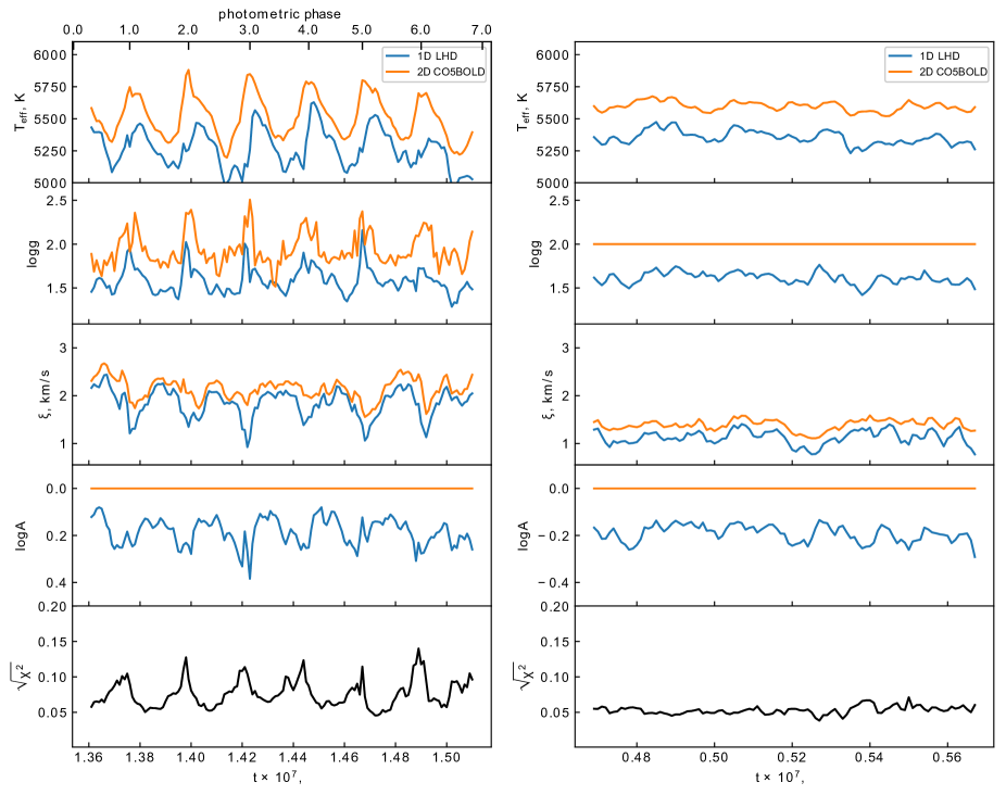
Figure 5: Result of the four-parametric fitting for the pulsating (left panel) and non-pulsating (right panel) regimes. The parameters of the 2D model are shown by orange lines for both regimes. The reconstructed parameters with the 1D LHD grid are shown by blue lines. The relative RMS deviation $\sqrt{\xi^{2}}$ in line strengths between the 2D and 1D models is shown by the black line.

The results of the four-parameter fitting when pulsations have set in are shown in the left panel of Fig. 5. There are significant biases between the 2D model parameters and the result of the fitting using 1D hydrostatic plane-parallel models. The mean bias in the determination of the effective temperature is $T_{\mathrm{teff}}^{2D}-T_{\mathrm{teff}}^{1D}\approx 250$ K, depending on the pulsation phase. During phases of the maximum compression, it is higher than 400-600 K, whereas it varies in a range from 100 K to 200 K for photometric phases $\phi_{\mathrm{ph}}\approx 0.3\ldots 0.65$, which correspond to the maximum expansion and early contraction stages. Gravity and metallicity exhibit mean biases between 2D and 1D values of roughly $0.35$ and $0.2$, respectively. The reconstructed microturbulent velocity is slightly lower (by $\approx 0.1$ kms^-1) than the 2D result, and shows a clear modulation with pulsational phase. We recall that the microturbulent velocity measured in the 2D case is not a result of the standard spectroscopic measurement of $\xi_{\mathrm{t}}$ (see details in Paper I), and neither is our fitting result based on least squares. In view of what to expect during an observational analysis, the bias of the microturbulence should therefore be taken as only indicative.

As stated before, the square root of the $\chi^{2}$ function in Fig. 5 characterizes the mean relative difference between EWs of the 2D and 1D LHD model. Depending on the photometric phase, this quantity varies from 5 % to 20 %. For the most extreme cases at maximum compression, the difference is the largest.

It might be argued that pulsations mainly disturb the thermal structure of the 2D model, and physical conditions in the line-formation region differ from the hydrostatic case. To check this hypothesis, the fitting was made for the case when pulsations have not set in. The result of the fitting is shown in the right panel of Fig. 5. For this regime, the relative difference in EWs is only 4-7 %, but the mean biases of the stellar parameters are very similar as in the time interval when pulsations have set in. We conclude that the pulsations contribute additional perturbations during the phase of maximum compression, but the main disturber of the thermal structure is convection (see also Paper I for further discussion).

Biases in the determination of stellar parameters for the cases when pulsations have and have not set in are caused by significant differences in the EWs of the 2D model and 1D LHD models. As we remarked above, this is caused by the different thermal structures of these models in the line-formation region. Thermal structures of the mean 2D model, which are the result of horizontally averaging over Rosseland optical depth, and 1D models are shown in Fig. 6. The 1D models were chosen from the grid according to the results of the fitting for the non-pulsating regime, taking the effective temperature to be $T_{\mathrm{eff}}=5300,5400$ K, and gravity $\log\,g=1.5,1.7$ dex. Additionally, we plot the 1D LHD model with 2D nominal surface gravity and effective temperature. To simplify the discussion, we only consider the non-pulsating stage of the temporal evolution of the 2D model.

The temporal variation of the horizontally averaged structure of the 2D model is indicated by the light blue region. The photospheric temperature of the 2D model changes as a result of convection. Convective overshoot and downflows produce the bump in the thermal structure at $\log\tau_{\mathrm{R}}=0$. Convective regions of the 1D LHD models are located below the photosphere, and MLT cannot reproduce this particular thermal profile. We have calculated thermal profiles with different mixing length parameters, but there are no qualitative improvements. The 1D LHD model with the same effective temperature $T_{\mathrm{eff}}=5600$ K and gravity $\log\,g=2.0$ as the 2D model has appriximately the same temperature profile in a range of optical depths from $\log\,\tau_{\mathrm{R}}=-3$ to $\log\,\tau_{\mathrm{R}}=-1$. The 2D model has a lower temperature for $\approx 250$ K at $\log\,\tau_{\mathrm{R}}\approx 0$ than the 1D LHD model, however. The fitting reconstructs the photospheric temperature. Because it has the same photospheric temperature, the 1D model has a cooler temperature profile in the line formation regions than the 2D model.

For the EW $W$ of a weak line, the following expression holds (Gray, 1992):

$$W_{\mathrm{\lambda}}\sim\int\frac{l(\lambda)}{\kappa(\lambda)}d\lambda,$$ (9)

where $l$ and $\kappa$ are the line and continuous absorption coefficients, respectively. For the range of the effective temperature of the 2D model between 5200 K and 5800 K, the negative hydrogen ion $\mathrm{H}^{-}$ is the dominant source of continuous opacity, and it is very sensitive to temperature. Iron is mostly ionized in this temperature range. Thus, neutral iron is a minority species, and its EWs increase with a decrease in effective temperature because the $\mathrm{H}^{-}$ opacity drops (Eq. 9). However, the behavior of singly-ionized iron EWs as a function of temperature is opposite to that of neutral iron. For any snapshot of the non-pulsating sequence, we can calculate EWs of the 1D LHD model taking the effective temperature, surface gravity, microturbulent velocity, and metallicity of the 2D model. Our calculation shows a mean relative difference of 13 % between the 2D and 1D model EWs because the photospheric regions of $\log\leavevmode\nobreak\ \tau_{\mathrm{R}}\sim 0$ in the 2D model are cooler than in the 1D LHD model. Specifically, (i) the 1D LHD model EWs of Fe i lines $W_{\mathrm{{Fe\textsc{i}}}}^{\mathrm{1D}}$ are lower than $W_{\mathrm{{Fe\textsc{i}}}}^{\mathrm{2D}}$, $W_{\mathrm{{Fe\textsc{i}}}}^{\mathrm{1D}}<W_{\mathrm{{Fe\textsc{i}}}}^{\mathrm{2D}}$, and (ii) the EWs of the Fe ii lines in the 1D model are larger than the 2D model EWs, $W_{\mathrm{{Fe\textsc{ii}}}}^{\mathrm{1D}}>W_{\mathrm{{Fe\textsc{ii}}}}^{\mathrm{2D}}$.

From a physical point of view, EWs of Fe i lines are most sensitive to changes of the effective temperature, and rather insensitive to changes of the gravity. However, EWs of Fe ii lines have the opposite behavior: they are sensitive to changes of the gravity, and less sensitive to changes of the temperature. So, in a first qualitative fitting step, one has to decrease the effective temperature and surface gravity of the 1D LHD model to transform (i) and (ii) toward similar differences in relative EWs $(W^{\mathrm{2D}}-W^{\mathrm{1D}})/W^{\mathrm{2D}}$ for all ionization stages. The procedure increases EWs of the 1D LHD model with respect to $W^{\mathrm{2D}}$. As a result, one has to decrease the metallicity to reduce the difference $(W^{2D}-W^{1D})$ in a second step. It leads to a lower metallicity in the fit for the pulsating as well as non-pulsating phases.

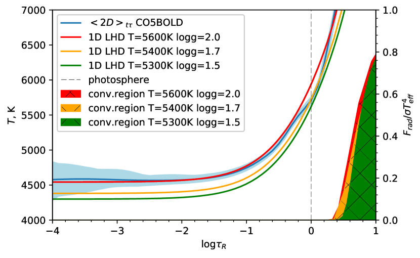
Figure 6: Comparison of the thermal structures of the horizontally (on surfaces of constant optical depth) averaged 2D model 1D models for the case when pulsations have not set in. The mean 2D thermal structure varies during 99 instances in time within the light blue region. The temporally averaged 2D profile is shown in blue.

7.2 Three-parameter case

In an observational analysis, the dimensionality of the parameter space is typically reduced using additional information. Gray & Johanson (1991) developed a method for determining the effective temperature using the line depth ratios of pairs of weak lines of the same chemical element with two different excitation potentials for G and K dwarfs. These ratios are sensitive to the temperature variation and independent of metallicity effects for weak lines (Gray, 1994). Kovtyukh & Gorlova (2000) extended this method to derive precise temperatures of classical Cepheids and yellow supergiants with 10-15 K internal uncertainty using a calibration of the line depth ratio versus effective temperature for 32 line pairs. Andrievsky et al. (2002b); Lemasle et al. (2007); Luck et al. (2011) used this calibration or the updated version (Kovtyukh, 2007) to derive the effective temperatures of Galactic Cepheids.

The surface gravity can be estimated through the condition of the ionization balance, but for this, the correct effective temperature is required because the EW is quite sensitive to temperature changes. Now we assume the effective temperature to be known, and set to the value of the 2D model for each particular instance in time. The effective temperature being fixed, we estimate the three remaining parameters. One-dimensional EWs were interpolated in the $\log\,g$-$\xi_{\mathrm{t}}$-$\log\,A$ space for the fixed effective temperature. The results of the three-parametric fitting for the non-pulsating and pulsating stages of the temporal evolution are shown in the right and left panels of Fig. 7, respectively. The gravity estimate in the three-parameter fitting is based on the ionization balance, which is hidden in the comparison of EWs of Fe i and Fe ii lines. In the range of effective temperatures of the 2D model, most of the iron is in the singly-ionized state. Weak lines of Fe i are insensitive to pressure changes and, thus, to variations of the effective gravity. Conversely, singly-ionized iron is pressure sensitive because of the opacity change in the negative hydrogen ion, which is sensitive to the electron pressure, giving an overall dependence (Gray, 1992)

$$W_{{Fe\textsc{ii}}}\sim g^{-\frac{1}{3}}.$$ (10)

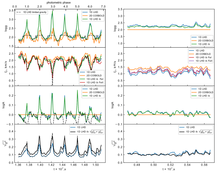
Figure 7: Result of the three-parameter fitting for the pulsating (left panel) and non-pulsating (right panel) regimes. The parameters of the 2D model are shown by orange lines for both regimes. The reconstructed parameters with the direct three-parameter fitting using the 1D LHD grid are shown by blue lines. Results using the ionization balance are shown by green, brown, and solid black lines. For the pulsating regime, the result of the experiment with a gravity limit for the maximum compression phase is shown by the dashed black line. The relative RMS deviation $\sqrt{\chi^{2}}$ in line strengths between the 2D and 1D models is shown by the solid blue and black lines for the direct three-parameter fitting and for a fitting using the ionization balance condition, respectively.

In addition to the simultaneous fit in all three parameters, we also derived the gravity by enforcing ionization balance. For each instance in time, we considered a two-parameter fit $\{\xi_{t},\log\ A\}$ of the Fe i and Fe ii lines separately, where the gravity was varied on the grid between $0.7\ldots 3.5$ dex. The estimation of the surface gravity using the ionization balance condition was based on deriving the same abundance for Fe i and Fe ii. Figure 7 shows that the results of the fit using the ionization balance condition and the direct fit of all three parameters are in good agreement.

In comparison to the four-parameter case, the reconstructed microturbulent velocity is very similar and consequently shows the same bias of $\approx-0.1$ kms^-1. The average microturbulent velocity estimated from the ionization balance coincides with the result of the full three-parameter fit for the pulsating and non-pulsating regimes. The metallicities derived for the non-pulsating regime closely correspond to the input value of the 2D model. The convection effect leads to a small variation in $\log\,A$ with time. It ranges between -0.03 and 0.04 dex.

For the regime when pulsations have set in, there is a deviation 0.25 dex in metallicity for the photometric phase with the maximum compression. Just after the maximum compression phase, there is a time interval exhibiting the smallest offset in metallicity stretching in the photometric phase between $\phi_{\mathrm{ph}}\approx 0.3\ldots 0.65$. From a physical point of view, this photometric phase coincides with the times of maximum expansion and subsequent start of compression. During this period, the atmosphere is in a levitating state, and convection and its disturbances of the thermal structure are not as strong as during maximum compression. The atmosphere is roughly in hydrostatic equilibrium, and the 1D models reasonably reproduce the mean thermal structure of the line formation region of the 2D model. This is shown in Fig. 8 for the photometric phases 0.25 and 0.6. It leads to a correct reconstruction of the metallicity with a 10 % relative difference between $W^{\mathrm{1D}}$ and $W^{\mathrm{2D}}$.

For the phase of maximum compression, the thermal structures of 1D and mean 2D model in line formation regions differ appreciably despite the fact that they have the same effective temperatures. At optical depths $\log\,\tau_{\mathrm{R}}\approx-1.3$, the mean 2D structure is 400 K cooler than the fitted 1D structure. The 2D structure has a rather low resolution of the optical depth scale around $\tau_{\mathrm{R}}\sim 1$ and exhibits steep temperature gradients. For the 2D model, the horizontal averaging on surfaces of constant optical depth yields lower temperatures for the photospheric regions. However, experiments with increased resolution of the optical depth scale using interpolation and subsequent horizontal averaging did not yield a qualitative change of the mean 2D structure. This suggests that the horizontal inhomogeneities produced by convection and the horizontal averaging leads to the lower photospheric temperatures in comparison to 1D. In addition, the large changes in opacities on the coarse numerical grid and the steep temperature gradients might contribute as well. This has to be tested in future simulations with higher numerical resolution.

As we described above, the Fe I lines are insensitive to the surface gravity. A high effective gravity of the 2D model leads to a decrease in Fe II EWs $W^{\mathrm{2D}}_{{Fe\textsc{ii}}}$ according to Eq. (10). For the spectral synthesis with 1D LHD models of fixed effective temperature, the surface gravitiy has to be increased in a first qualitative fitting step to obtain the relative difference $(W^{\mathrm{2D}}_{{Fe\textsc{ii}}}-W^{\mathrm{1D}}_{{Fe\textsc{ii}}})/W^{\mathrm{2D}}_{{Fe\textsc{ii}}}$ similar to Fe i. Owing to different thermal structures of the line formation regions, 1D EWs are smaller than the corresponding values of the 2D model. As a second step, the iron abundance therefore has to be increased to minimize the differences in EW. This leads to a positive bias for the metallicity during the phase of maximum compression and to high values of the reconstructed gravity.

To understand the effect of the gravity on the metallicity bias during the phase of maximum compression, we performed an additional test. For this phase, the gravity was limited to $\log\,g=2.1$ or less. The results of the fitting are shown for the case when pulsations have set in in the left panel of Fig. 7. For a better fitting of the 2D EWs, the metallicity or microturbulent velocity can be changed. However, EWs of weak lines are insensitive to the change in microturbulent velocity. Thus, to reduce the difference $(W^{2D}-W^{1D})$, the metallicity has to be decreased.

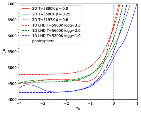
Figure 8: Comparison of thermal structures of LHD models with the mean temperature profiles (average over optical depth surfaces) of the two-2D model for several photometric phases. $\tau_{\mathrm{R}}$ is the Rosseland optical depth.

7.3 Two-parameter case

We now assume that the effective temperature and the effective gravitational acceleration are known from independent considerations. We take the effective temperature and gravity of the 2D model and interpolate EWs calculated with the grid of 1D models in $\xi_{\mathrm{t}}$-$\log\,A$ space. In this two-parameter case, $\chi^{2}$ is a function of the microturbulent velocity and metallicity alone.

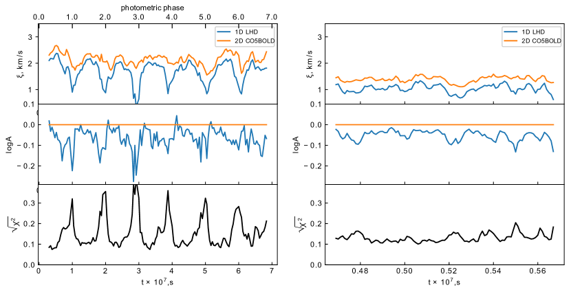
Figure 9: The result of the three-parametric fitting for the pulsating (left panel) and non-pulsating (right panel) regimes. The parameters of the 2D model are shown by orange lines for both regimes. The reconstructed parameters with the 1D LHD grid are shown by blue lines. The relative RMS deviation $\sqrt{\chi^{2}}$ in line strengths between the 2D and 1D models is shown by black line.

Again, we performed the two-parameter fit for the pulsating and non-pulsating stages of the temporal evolution of the 2D model. The results are shown in the left and right panels of Fig. 9. The effective gravity of the 2D model for the pulsating case is lower than the values of the three-parameter fitting. As we showed in the previous subsection, the lower gravity leads to a negative bias of the metallicity for most phases, except for the phase of the maximum expansion and start of the contraction. For this phase, the result of the fitting shows a perfect reconstruction of the metallicity because the atmosphere is close to hydrostatic conditions, and the 1D model can reproduce the thermal structure (see Fig. 6). When pulsations have not set in, the reconstructed mean metallicity is $\log\,A^{\mathrm{1D}}=-0.05$ dex, which is lower than the result of the three-parameter fit because the gravity is fixed to $\log\,g=2$. According to Eq. (10), this leads on average to higher EWs in 1D, and hence to a slight decrease of the metallicity.

Owing to the smaller number of free parameters in the two-parameter case, the $\sqrt{\chi^{2}}$ value increases to a level of $\approx 10$ %, except for the phases of maximum compression. When the analysis of the spectra is performed by taking some random photometric phase, a negative metallicity bias of $\approx 0.06$ dex is obtained on average.

7.4 Connection between abundance and EW fitting

We minimized a $\chi^{2}$ function of up to four parameters, which is the sum of relative differences of the individual line EWs between the 2D model and 1D models. Here we wish to provide arguments as to why the fitting in EW does not give a qualitatively different result when the fitting of line-by-line abundances is considered. With fixed effective temperature and gravity, we reconstructed the thermal structure of the line formation regions. The minimization of the mean difference of $W^{\mathrm{2D}}$ and $W^{\mathrm{1D}}$ EWs is equal to the minimization of the mean abundance differences $A^{\mathrm{2D}}-A^{\mathrm{1D}}$. This can be shown analytically for weak lines. For the two-parameter case, when $\chi^{2}$ is a function of the microturbulent velocity and abundance, we obtain

$$\chi^{2}(A,\xi_{\mathrm{t}})=\frac{1}{N}\sum_{\mathrm{i}}^{N}\left[\frac{W^{\mathrm{2D}}_{\mathrm{i}}-W^{\mathrm{1D}}_{\mathrm{i}}(A,\xi_{\mathrm{t}})}{f\cdot\sigma_{\mathrm{W,i}}}\right]^{2},$$ (11)

where N is the number of lines. To first order, the difference in EWs of the line $i$ between the 2D 1D model can be represented by the Taylor expansion

$$W^{\mathrm{2D}}_{\mathrm{i}}-W^{\mathrm{1D}}_{\mathrm{i}}\approx\frac{\partial W_{\mathrm{i}}}{\partial\xi_{\mathrm{t}}}\cdot(\xi_{\mathrm{t,i}}^{\mathrm{2D}}-\xi_{\mathrm{t,i}}^{\mathrm{1D}})+\frac{\partial W_{\mathrm{i}}}{\partial A}\cdot(A_{\mathrm{i}}^{\mathrm{2D}}-A_{\mathrm{i}}^{\mathrm{1D}})+\ldots.$$ (12)

The uncertainty $\sigma_{\mathrm{W,i}}$ in the EW is related with uncertainties in the abundance $\sigma_{\mathrm{A,i}}$ and microturbulent velocity $\sigma_{\mathrm{\xi_{\mathrm{t}}}}$

$$\sigma_{\mathrm{W,i}}=\sqrt{\left[\frac{\partial W}{\partial\xi_{\mathrm{t}}}\right]^{2}\sigma^{2}_{\mathrm{\xi_{\mathrm{t}}i}}+\left[\frac{\partial W}{\partial A}\right]^{2}\sigma^{2}_{\mathrm{A,i}}}.$$ (13)

Weak lines are insensitive to change in $\xi_{\mathrm{t}}$. Inserting the condition $\frac{\partial W}{\partial\xi_{\mathrm{t}}}=0$ into Eqs. (13) and  (12), we can modify Eq. (11)

$$\chi^{2}\approx\frac{1}{N}\sum_{\mathrm{i}}^{N}\left[\frac{A^{\mathrm{2D}}_{\mathrm{i}}-A^{\mathrm{1D}}}{f\cdot\sigma_{\mathrm{A,i}}}\right]^{2},$$ (14)

which shows that the minimization of the difference of EWs is equal to minimizing the difference in abundance between the 1D grid and 2D model.

7.5 Comparison of EWs

Using the curve of growths, we can transform the difference in EWs $W^{\mathrm{2D}}-W^{\mathrm{1D}}$ into an abundance correction for each individual line. The individual abundance corrections as a function of the line strength and photometric phase are shown in Fig. 10 for the three-parameter case. As expected, the smallest abundance corrections correspond to photometric phases $\phi_{\mathrm{ph}}\approx 0.3\ldots 0.65$. Generally, Fe i lines have larger abundance corrections than Fe ii lines. Additionally, within the same ionization stage, the abundance corrections become smaller with increasing excitation potential.

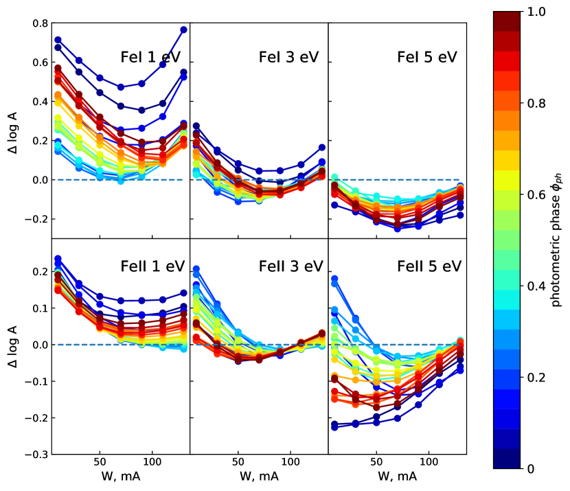
Figure 10: Abundance corrections for individual lines for the best-fitting 1D models as a function of line strength and photometric phase.

8 Summary and conclusion

We have determined the stellar parameters (effective temperature, gravity, microturbulent velocity, and metallicity), of a 2D dynamical Cepheid model that was calculated with the CO5BOLD code and has been presented in Paper I. We took EWs based on the 2D model as observational data and calculated a grid of the 1D plane-parallel hydrostatic model atmospheres for two regimes of the temporal evolution of the 2D model. We performed the analysis for three different cases:

1. A four-parameter case, where $\chi^{2}$ is a function of $T_{\mathrm{eff}},\log\,g,\xi_{\mathrm{t}}$, and $\log\,A$. All reconstructed parameters are biased toward lower values than in the 2D model snapshots, and they are on average largely independent of the pulsations. The bias in the metallicity determination is $\approx-0.2$ dex.

2. A three-parameter case, where the $T_{\mathrm{eff}}$ is fixed to the 2D value. $\chi^{2}$ is a function of $\log\,g,\xi_{\mathrm{t}}$, and $\log\,A$. Stellar parameters are determined with (i) direct three-parameter fitting, and (ii) using the condition of ionization balance. The gravity estimate is higher than the effective 2D gravity for the pulsating and non-pulsating regimes. For the non-pulsating regime, the metallicity reconstruction agrees for all instances in time, whereas when pulsations have set in, only the photometric phases $\phi_{\mathrm{ph}}\approx 0.3\ldots 0.65$ show a slightly biased metallicity estimate.

3. A two-parameter case, where $\chi^{2}$ is a function of $\xi_{\mathrm{t}}$ and $\log\,A$. The metallicity estimate behaves qualitatively similar to case (2).

One-dimensional hydrostatic plane-parallel stellar model atmospheres employing different MLT formulations generally cannot reproduce the mean thermal structure of the 2D model for the whole range of optical depths. In particular, the temperature at optical depth unity of the 1D models is typically higher than for the mean 2D model. To avoid systematic biases in the determination of stellar parameters of Cepheids with standard model atmospheres, we recommend analyzing spectra taken during photometric phases $\phi_{\mathrm{ph}}\approx 0.3\ldots 0.65$.

Our investigation was based on a single dynamical model of a Cepheid, restricted to two spatial dimensions. A comprehensive theoretical investigation of the line formation in the atmospheres of Cepheid variables would require additional models, in particular, consideration of the full 3D case, and calculation of 2D models of higher numerical resolution as well as lower surface gravity, corresponding to longer pulsation periods. Including effects of sphericity and investigating departures from local thermodynamic equilibrium are desirable future improvements on the side of dynamical multidimensional modeling. From a technical point of view, it would be advantageous to use double precision because of the short radiative time step and, as a consequence of it, the very small relative changes of the model properties (particularly of the internal energy) between time steps.