A Study of Fermi-LAT GeV $\gamma$-ray Emission towards the Magnetar-harboring Supernova Remnant Kesteven 73 and Its Molecular Environment

Abstract

We report our independent GeV $\gamma$-ray study of the young shell-type supernova remnant (SNR) Kes 73 which harbors a central magnetar, and CO-line millimeter observations toward the SNR. Using 7.6 years of Fermi-LAT observation data, we detected an extended $\gamma$-ray source (“source A”) with centroid on the west of the SNR, with a significance of $21\sigma$ in 0.1–300 GeV and an error circle of $5.^{\prime}4$ in angular radius. The $\gamma$-ray spectrum cannot be reproduced by a pure leptonic emission or a pure emission from the magnetar, and thus a hadronic emission component is needed. The CO-line observations reveal a molecular cloud (MC) at $V_{\scriptscriptstyle\rm LSR}\sim 90\,{\rm km}\,{\rm s}^{-1}$, which demonstrates morphological correspondence with the western boundary of the SNR brightened in multiwavelength. The ${}^{12}{\rm CO}$ ($J$=2-1)/${}^{12}{\rm CO}$ ($J$=1-0) ratio in the left (blue) wing 85–88$\,{\rm km}\,{\rm s}^{-1}$ is prominently elevated to $\sim 1.1$ along the northwestern boundary, providing kinematic evidence of the SNR-MC interaction. This SNR-MC association yields a kinematic distance $9\,{\rm kpc}$ to Kes 73. The MC is shown to be capable of accounting for the hadronic $\gamma$-ray emission component. The $\gamma$-ray spectrum can be interpreted with a pure hadronic emission or a magnetar+hadronic hybrid emission. In the case of pure hadronic emission, the spectral index of the protons is 2.4, very similar to that of the radio-emitting electrons, essentially consistent with the diffusive shock acceleration theory. In the case of magnetar+hadronic hybrid emission, a magnetic field decay rate $\gtrsim 10^{36}\,{\rm erg}\,{\rm s}^{-1}$ is needed to power the magnetar’s curvature radiation.

1 Introduction

Cosmic rays (CRs) are relativistic particles that are mainly comprised of hadrons (protons and nuclei) with a small fraction of leptons. The origin of CRs remains a highly controversial issue as yet, although they have been known for more than a hundred years. During propagation, relativistic hadrons may interact with subrelativistic nuclei, producing $\pi^{0}$ mesons that will decay to $\gamma$-rays. Moreover, highly energetic leptons can produce $\gamma$-rays by inverse Compton (IC) scattering low-energy photons or by nonthermal bremsstrahlung emission. Thus, $\gamma$-ray observations can offer us crucial information to solve the puzzling issue. Supernova remnants (SNRs), known for tremendous energy contained in their strong shocks, are one of the most popular kinds of candidates for Galactic CR accelerators. Dozens of GeV $\gamma$-ray sources associated with SNRs have been discovered by the Fermi Large Area Telescope (LAT) in recent years (e.g., Abdo et al., 2009, 2010; Acero et al., 2016). However, it is still difficult to distinguish the radiation processes of the $\gamma$-rays (hadronic or leptonic) that are associated with SNRs, and it becomes more complicated for the SNRs with poorly characterized interstellar environments and associated compact object. In this paper, we will study the GeV $\gamma$-ray emission from the magnetar-harboring SNR Kesteven 73 (hereafter Kes 73) and its possible molecular environment.

Kes 73 (G27.4$+$0.0) is a young SNR with an incomplete shell both in radio and X-rays, filled with clumpy X-ray substructures (Helfand et al., 1994; Kumar et al., 2014). It hosts the magnetar 1E 1841$-$045 that was first identified as an anomalous X-ray pulsar (AXP) in the center (Vasisht & Gotthelf, 1997). The X-ray studies inferred that its forward shock has encountered the interstellar/circumstellar material (Kumar et al., 2014; Borkowski & Reynolds, 2017). The remnant is estimated to be young, of an age between 500 and 2100 years (Tian & Leahy, 2008; Kumar et al., 2014; Gao et al., 2016; Borkowski & Reynolds, 2017), while the characteristic age of the AXP is $\sim 4.7$ kyr. Its progenitor is suggested to be a massive star ($\gtrsim 20$ M_⊙, Kumar et al. 2014; $<20$ M_⊙, Borkowski & Reynolds 2017). Moreover, the distance to Kes 73 is a controversial issue. The distance estimated from the H i absorption is between $7.5$ and $9.8\,{\rm kpc}$ (Tian & Leahy, 2008). Use of a statistical method for pulsar distance measurement gives the distance to the central magnetar 1E 1841-045 as $8.2$–$10.2\,{\rm kpc}$ (Verbiest et al., 2012). In addition, the $\Sigma$-$D$ relationship suggests a distance of $\sim 14.8\,{\rm kpc}$ (Pavlovic et al., 2014).

Magnetars are a small group of X-ray pulsars comprised of AXPs and soft $\gamma$-ray repeaters, with strong magnetic fields. Pulsed GeV radiation has been expected to arise from the magnetospheres of magnetars (e.g., Cheng & Zhang, 2001; Beloborodov & Thompson, 2007; Takata et al., 2013). As for 1E 1841$-$045, its slow spin period (11.8 s) and rapid spin-down rate imply an extreme field strength, $\sim 7\times 10^{14}\ \rm G$, assuming the dipole spin-down model (An et al., 2013). In recent research, extended GeV $\gamma$-ray emission that is possibly associated with the Kes 73 SNR/AXP system was detected, while the origin of this diffuse $\gamma$-ray emission remains a controversial issue (Acero et al., 2016; Li et al., 2017; Yeung et al., 2017). In a GeV survey for magnetars, no significant detection of $\gamma$-ray flux or $\gamma$-ray pulsation from 1E 1841$-$045 has been found, and the stringent upper limit on the 0.1–10 GeV emission of the magnetar is $<2.02\times 10^{-11}$ erg cm^-2 s^-1 after the subtraction of the extended emission from the SNR (Li et al., 2017), while another Fermi-LAT study implied that the magnetar is seemingly a necessary and sufficient source for the downward-curved spectrum below 10 GeV (Yeung et al., 2017).

There are a few hints of dense gases such as molecular clouds (MCs) in the nearby region. The 1720 MHz OH line is detected projectively at $12^{\prime}$ west of the SNR at a local standard of rest (LSR) velocity $V_{\scriptscriptstyle\rm LSR}\sim+33\,{\rm km}\,{\rm s}^{-1}$ (Green et al., 1997) but it has been identified with a separate H ii region (Helfand et al., 1992). Observations in ${}^{13}{\rm CO}$ ($J=$1-0) and H i lines imply associated gas at $\sim 110\,{\rm km}\,{\rm s}^{-1}$ (Tian & Leahy, 2008). Broadened features in the ${}^{12}{\rm CO}$ ($J$=2-1) line are found from a region $\sim 2^{\prime}$–$4^{\prime}$ away from the SNR boundary and is conjectured to be caused by a disturbance due to the fast-moving ejecta (Kilpatrick et al., 2016).

In an independent study, we examine the GeV emission from the Kes 73 region using Fermi-LAT data and investigate the interstellar molecular environment of the SNR by millimeter CO-line observations toward the region. We focus on the spectral properties of the $\gamma$-ray emission and possible hadronic contribution resulting from the interaction between the SNR and the nearby MC and provide an estimate for the possible contribution from the magnetar. In the rest of this paper, we describe the $\gamma$-ray and millimeter observations and data reduction in §2, and present the data analyses and results in §3. We discuss the results in §4 and summarize this work in §5.

2 Observations and Data

2.1 Fermi-LAT Observational Data

The LAT on board Fermi is a $\gamma$-ray imaging instrument that detects photons in a broad energy range of 20 MeV to more than 300 GeV. Starting from the front of the instrument, the LAT tracker has 12 layers of thin tungsten converters (FRONT section), followed by four layers of thick tungsten converters (BACK section). Its per-photon angular resolution (point-spread function, PSF, the $68\%$ containment radius ) varies strongly with photon energy and improves a lot at high energies ($\sim 5\arcdeg$ at 100 MeV, and $0\fdg 8$ at 1 GeV, Atwood et al. 2009). In addition, the PSF for the FRONT events are approximately a factor of two better than the PSF for the BACK events.

In this research, we collected 7.6 years of Fermi-LAT Pass 8 data, from 2008-08-04 15:43:36 (UTC) to 2016-03-25 00:10:13 (UTC). We used the package Fermi ScienceTools version v10r0p5 released on 2015 June 24, to analyze the data in the energy range 0.1–300 GeV. We only selected Source (evclass$=$128) events within a maximum zenith angle of 90^∘ in order to filter out the background $\gamma$-rays from the Earth’s limb and applied the recommended filter string “($DATA\_QUAL>0)\&\&(LAT\_CONFIG==1$)” in gtmktime to choose the good time intervals. The corresponding instrument response functions (IRFs) are “P8R2_SOURCE_V6” for the total (FRONT+BACK) data and “P8R2_SOURCE_V6::FRONT” for the FRONT data.

2.2 CO Line Observations and Data

The observations in millimeter molecular lines toward SNR Kes 73 were made in two periods, both in position switching mode. The first observation was made in the ${}^{12}{\rm CO}$ ($J$=2-1) line (at 230.538  GHz) in 2010 January using the Kölner Observatory for Submillimeter Astronomy (KOSMA) 3m submillimeter telescope in Switzerland. A superconductor-insulator-superconductor (SIS) receiver was used as the front end, and an acousto-optical spectrometer (AOS) was used as the back end. We mapped a $15^{\prime}\times 15^{\prime}$ area covering Kes 73 centered at (${18}^{{\rm h}}{41}^{{\rm m}}{17}^{\rm s}.3$, ${-4}^{\circ}{56}^{\prime}{17}^{\prime\prime}.0$, J2000) with grid spacing $1^{\prime}$ and the reference position is at (${18}^{{\rm h}}{41}^{{\rm m}}{19}^{\rm s}.2$, ${-4}^{\circ}{56}^{\prime}{11}^{\prime\prime}.0$, J2000). The half-power beam width (HPBW) of the telescope is $130^{\prime\prime}$, and the main beam efficiency is $\eta_{mb}\sim 68\%$.

The follow-up observation was made in the ${}^{12}{\rm CO}$ ($J$=1-0) line (at 115.271  GHz), the ${}^{13}{\rm CO}$ ($J$=1-0) line (at 110.201  GHz), and the ${\rm C}^{18}{\rm O}$ ($J$=1-0) line (at 109.782  GHz) in 2014 April using the 13.7 m millimeter-wavelength telescope of the Purple Mountain Observatory at Delingha (hereafter PMOD), China. At the front end, there is a $3\times 3$ pixel Superconducting Spectroscopic Array receiver, which was made with SIS mixers using the sideband separating scheme (Zuo et al., 2011; Shan et al., 2012). An instantaneous bandwidth of 1  GHz was arranged for the back end. Each spectrometer provides 16,384 channels with total bandwidth of 1000  MHz and the velocity resolution was $0.158\,{\,{\rm km}\,{\rm s}^{-1}}$ and $0.166\,{\,{\rm km}\,{\rm s}^{-1}}$ for the ${}^{12}{\rm CO}$ and ${}^{13}{\rm CO}$  lines, respectively. We mapped a $45^{\prime}\times 45^{\prime}$ area covering Kes 73 centered at ($27\fdg 5,0\fdg 0$) in the Galactic coordinate system with a grid spacing $\sim 30^{\prime\prime}$ and the reference position is at ($27\fdg 5,0\fdg 0$). The HPBW of the telescope is $52^{\prime\prime}$ and the main beam efficiency is $\eta_{mb}\sim 52\%$.

All the CO data were reduced with the GILDAS/CLASS package developed by IRAM. The intensity scales were calibrated using the standard chopper-wheel calibration method (e.g., Ulich & Haas, 1976) for molecular lines. Thus the intensity derived is the one corrected for the atmospheric and ohmic attenuation. For extended sources, this intensity needs further correction by the main beam efficiency $\eta_{mb}$ to yield an observational radiation temperature. The mean RMS noise levels of the main beam brightness temperature are about 0.5 K, 0.2 K, and 0.2 K for the ${}^{12}{\rm CO}$ ($J$=1-0), ${}^{13}{\rm CO}$ ($J$=1-0) and ${}^{12}{\rm CO}$ ($J$=2-1) lines, respectively.

In addition, we also used the ${}^{12}{\rm CO}$ ($J$=3-2) data from the second release (R2) data of the CO High-Resolution Survey (COHRS) of the James Clerk Maxwell Telescope (Dempsey et al., 2013).

2.3 Other Data

In order to compare the distribution of molecular material in the environs of Kes 73 with the morphology of the SNR, we used the archival Chandra X-ray data (ObsID: 729), the NRAO VLA Sky Survey (NVSS, Condon et al. 1998) 1.4  GHz radio continuum emission data and the Wide-field Infrared Survey Explorer (WISE, Wright et al. 2010) Band 4 ($22\,\mu{\rm m}$) mid-infrared (IR) all-sky survey data.

3 Multiwavelength Data Analysis and Results

3.1 Fermi-LAT $\gamma$-rays

Following the standard binned likelihood analysis procedure, the Fermi-LAT data analyses were applied to the $14\arcdeg\times 14\arcdeg$ (in equatorial coordinate system) region of interest, which is centered at the position of Kes 73, i.e., R.A. = 18^h41^m19^s, decl. = $-4^{\circ}55^{\prime}59^{\prime\prime}$ (J2000). The baseline model was generated by the user-contributed program make3FGLxml.py. It includes all the Third Fermi-LAT Catalog (3FGL) sources (Acero et al., 2015) within radius 15^∘ centered at Kes 73 and diffuse background, which consists of both the Galactic and extragalactic components (as specified in the files gll_iem_v06.fits and iso_P8R2_SOURCE_V6_v06.txt, respectively).

3.1.1 Detection and Localization

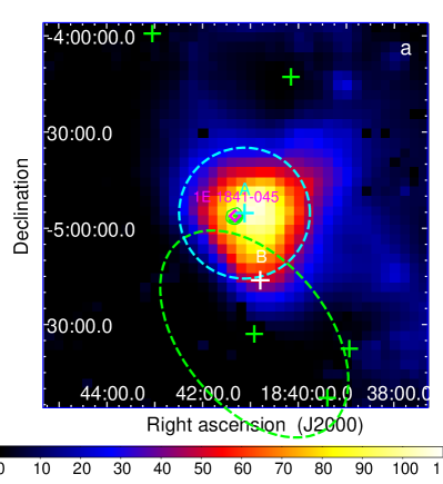
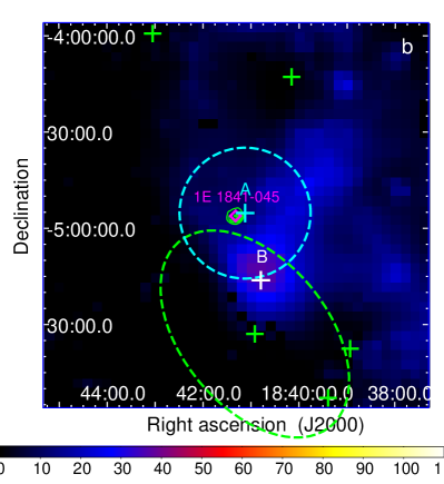
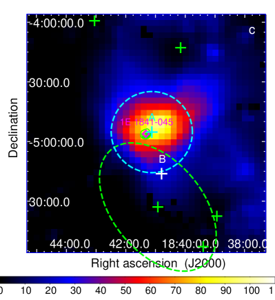
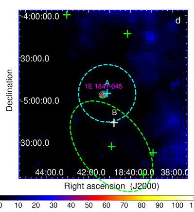
Figure 1: TS maps (1–300 GeV) of a $2^{\circ}\times 2^{\circ}$ region centered at Kes 73. The image scale of the map is $0\fdg 05$ pixel^-1. (a) All sources in the baseline model have been included. (b) All sources in the baseline model as well as source A (as a point source) have been included. (c) All sources in the baseline model as well as source B have been included. (d) All sources in the baseline model as well as source A (as an extended source) and B have been included. The green crosses label the positions of 3FGL sources, the cyan cross labels the best-fit position of source A, and its best fitted disk template is shown with a dashed cyan circle. The white cross indicates the location of an additional source (B) we added in the source model (for details, see §3.1.1). The magenta diamond represents the location of 1E 1841$-$045. The image is overlaid with NVSS 1.4 GHz radio continuum contours. The dashed-green oval depicts the spatial template of the extended 3FGL source HESS J1841$-$055.

At first, a binned likelihood analysis (using gtlike, a tool in the ScienceTools package) was applied in the energy range 1–300 GeV. In order to search for indications of $\gamma$-ray emission that is probably associated to Kes 73, we generated a Test Statistic (TS) map for a $2^{\circ}\times 2^{\circ}$ region centered at Kes 73 (see Figure 1). The TS value is defined as $2(\log{\mathcal{L}}/{\mathcal{L}}_{0})$, where ${\mathcal{L}}_{0}$ is the likelihood of null hypothesis and ${\mathcal{L}}$ is the likelihood with a test source included at a given position. As shown in Figure 1a, with all components in the baseline model treated as the background, the TS value around SNR Kes 73, especially on its western side, was quite high ($\sim 110$), implying lots of residual $\gamma$-ray emission in this area. To approximate the residual $\gamma$-ray emission, we added a point source with a simple power law (PL) spectrum to the baseline model at the TS peak position. Then we applied another binned likelihood analysis in the energy range 1–300 GeV on the newly updated source model. Next, we ran gtfindsrc (a tool in the ScienceTools package) and located the best-fit position of the newly added source (hereafter source A) at R.A.= 18^h 41^m 07${}^{\rm s}\!$, decl.= $-$4^∘ 55^′ 19${}^{\prime\prime}\!$ (J2000) with a 68% confidence error circle of $5.^{\prime}4$ in angular radius. For the following analyses, the center of source A is fixed in this position.

Next, to find out whether such a point source could well approximate the residual emission or not, we generated another TS map centered at Kes 73 with the contribution from the newly added source subtracted. As can be seen from Figure 1b, the TS value to the southwest of Kes 73 was still high ($>25$), implying many residual $\gamma$-rays that might come from another unknown $\gamma$-ray source.. To test this hypothesis, we performed similar procedures to those for the detection and localization of source A. By adding another point source (hereafter source B) with a PL spectrum at the peak position in the latter TS map, we adjusted the model and performed another binned likelihood analysis in the energy range 1–300 GeV. Then we located the best-fit position of source B at R.A.=${18}^{{\rm h}}{40}^{{\rm m}}{47}^{\rm s}$, decl.= ${-5}^{\circ}{16}^{\prime}{13}^{\prime\prime}$ (J2000) with a 68% confidence error circle of $3^{\prime}.0$ in angular radius utilizing gtfindsrc. With the two point sources (A and B) added to the baseline model, the residual emission was then found to be negligible and the value of the likelihood function increases significantly. In the energy range 1–300 GeV, the significance is $\sim 10.2\sigma$ for source A and $\sim 8.8\sigma$ for source B, with both assumed to be point sources.

In the above procedures, adding source A improves the source model likelihood by 121.7, and additionally adding source B further improves the likelihood by 21.2. Compared with source A, which is almost coincident with SNR Kes 73; however, source B seems to be far ($21.^{\prime}6$ projectively) away from the SNR. Therefore, we made another TS map (Figure 1c) with source B included in the model as a background source.

3.1.2 Spatial Analysis

As shown in Figure 1c, the residual emission coincident with Kes 73 looks diffuse rather than point-like. It was thus necessary to test the extension of source A. Using the definition and method in Lande et al. (2012), we modeled the surface brightness profile for an extended source as a uniform disk. The tested radius range for uniform disk models is $0\fdg 2-0\fdg 4$ with a step of $0\fdg 02$. We performed a likelihood-ratio test by comparing the likelihood of a uniform disk hypothesis (${\mathcal{L}}_{\rm disk}$) with that of point-source hypothesis (${\mathcal{L}}_{\rm point}$) to test the significance of extension. The $\gamma$-ray source was considered to be significantly extended only if ${\rm TS}_{\rm ext}$, defined as $2\log({\mathcal{L}}_{\rm disk}/{\mathcal{L}}_{\rm point})$, was $\geq 16$. We listed the ${\rm TS}_{\rm ext}$ values obtained from the uniform disk models with various radii in Table 1. The highest ${\rm TS}_{\rm ext}$, $40.1$ (corresponding to a significance of $\sim 6.3\sigma$) is achieved when the disk radius is $0\fdg 34^{+0\fdg 06}_{-0\fdg 04}$ . As shown in Figure 1d, with source A, source B, and other 3FGL background sources included in the background model, the residual emission is ignorable. Thus, in the following analyses, the $\gamma$-ray emission of source A is treated as an extended source (of which the centroid appears on the west of the SNR) and source B as a point source, and the $\gamma$-ray emission significances in the energy range 1–300 GeV for them are $\sim 13.3\sigma$ and $\sim 7.3\sigma$, respectively.

3.1.3 Spectral Analysis

We then performed a spectral analysis for a diagnostic of the physical property of source A. During this process, only FRONT events of energy ranging from 0.1 to 300 GeV were selected to lessen the contamination from nearby sources.

We first fit the 0.1–300 GeV spectral data of source A with a PL model. Under this assumption, the TS value of source A is 467.5, corresponding to a significance of $21.6\sigma$, and the obtained spectral shape is relatively flat with a photon index of $\Gamma=2.21\pm 0.06$. The flux is $(6.11\pm 1.14_{\rm stat}\pm 1.69_{\rm sys})\times 10^{-11}\,\mbox{erg}\,{\rm cm}^{-2}\,{\rm s}^{-1}$, corresponding to a luminosity of $\sim 5.9\times 10^{35}d_{9}^{2}$ erg s^-1, where $d_{9}=d/9$kpc is the distance to SNR Kes 73 in units of a reference value 9 kpc (see § 4.1 for details).

Next, we examined other possible spectral models, such as an exponentially cutoff power law (PLEC), a log-parabola model (LogP), and a broken power law (BKPL), and performed likelihood-ratio tests between the PL model (as the null hypothesis) and the other spectral models, parameterized with index TS${}_{\rm model}=2\log({\mathcal{L}}_{\rm model}/{\mathcal{L}}_{\rm PL})$. The functional forms for these models are presented in Table 2, while the fitting results were tabulated in Table 3. The TS_PLEC value $-4.4$ indicates that an additional exponential cutoff (typical for a pulsar) does not improve the fitting results compared to the pure PL model. We find TS${}_{\rm LogP}=6.7$ and TS${}_{\rm BKPL}=14.4$, with corresponding significance of $\sim 2.6\sigma$ and $\sim 3.8\sigma$, respectively, indicate a possibility for a curved spectrum or a spectral steepening above $\sim 1$ GeV. However, these two TS values are below the threshold 16, not high enough for the latter two models to replace the PL model.

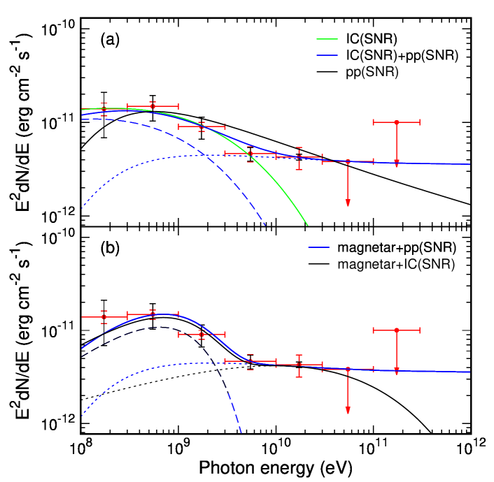
Figure 2: Fermi $\gamma$-ray SED of Kes 73, fitted with various models (see §4.3). Systematic errors (see §3.1.3) are indicated by black bars, and the statistical errors are indicated by red bars. In the upper panel, the long-dashed and short-dashed lines indicate the IC and p-p interaction components of Model I, respectively. In the bottom panel, the long-dashed line represents the magnetar emission in both Model III and Model IV; the short-dashed blue and black lines indicate the p-p interaction component in Model III and the IC component in Model IV, respectively.

The spectral energy distribution (SED) of source A was extracted via the maximum likelihood analysis of the FRONT events in seven divided energy bands from 0.1 to 300 GeV (see Table 4). The spectral normalization parameters of the sources within $5^{\circ}$ of Kes 73 and the diffuse background components were set free, while all the other parameters were fixed. In order to estimate the possible systematic errors caused by the imperfection of the Galactic diffuse background model, we artificially varied the normalization of the Galactic diffuse background by $\pm 6\%$ from the best-fit values in each energy bin (Abdo et al., 2009). The maximum deviations of the flux due to these changes in the Galactic diffuse background intensities were considered as the systematic errors. The resultant $\gamma$-ray spectrum is given in Figure 2.

3.1.4 Timing analysis

To search for long-term variability in source A, we follow the method described in Nolan et al. (2012) and calculate its Variability_Index (${\rm TS}_{\rm var}$) by dividing FRONT events in the energy range 0.1$-$300 GeV into approximately monthly time bins. If the flux is constant, then ${\rm TS}_{\rm var}$ is distributed as $\chi^{2}$ with 90 degree of freedom, and variability would be considered probable if ${\rm TS}_{\rm var}$ exceeds the threshold 124.1 corresponding to 99$\%$ confidence. The ${\rm TS}_{\rm var}$ of source A with all 91 time bins in 0.1$-$300 GeV is 98.9. Therefore, there is no significant long-term variability detected in source A.

In an attempt to explore the origin of the $\gamma$-ray emission of source A, we searched in the SIMBAD Astronomical Database (Wenger et al., 2000) within the $3\sigma$ error circle of the source for possible candidates of its counterpart(s). Among all the known objects (stars, MCs, H ii region, etc) in this area, SNR Kes 73 or the Kes 73 /1E 1841$-$045 system is most likely to be associated to the $\gamma$-ray emission given the GeV $\gamma$-ray analysis results.

3.1.5 Comparison with Previous Research

The detection of the GeV-bright extended source, “source A”, through the Fermi data analyses, confirms the discovery reported previously (Acero et al., 2016; Li et al., 2017; Yeung et al., 2017). But our analysis has some differences from theirs. In Li et al. (2017), on the assumption that the extended $\gamma$-ray emission is produced only by the SNR, they obtained a stringent upper limit on the 0.1–10 GeV emission of 1E 1841$-$045 ($<2.02\times 10^{-11}$ erg cm^-2 s^-1) via adding a point source at the position of 1E 1841$-$045. Taking a different approach, Yeung et al. (2017) treated these diffuse $\gamma$-rays as a combination of the contribution from SNR Kes 73 and magnetar 1E 1841$-$045, and performed spectral analyses of the source (Fermi J1841.1$-$0458 therein) in two energy bands (0.1–-10 GeV and 10–-200 GeV) separately.

In our analysis, the centroid of the extended source A is located to the west of the SNR, nearly on the western edge of the SNR, which is offset from the centroid of Fermi J1841.1$-$0.458. The angular radius of source A is a bit larger than that of Fermi J1841.1$-$0.458. Moreover, our spectral analysis was performed on the whole energy band (0.1–300 GeV) instead of dividing them into two energy band (0.1–10 GeV and 10–200 GeV). Also, we added source B as a background source. Due to these different treatments, the flux of source A that we obtained in 0.1–10 GeV is a bit lower than the flux of Fermi J1841.1$-$0.458 reported by Yeung et al. (2017).

3.2 CO Line Emission

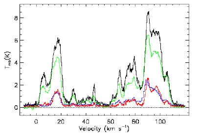
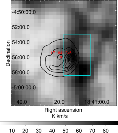
Figure 3: Left: average CO spectra from a $3.5^{\prime}\times 5.5^{\prime}$ region centered at R.A.$=18^{h}41^{m}10^{s}.7$, decl.$=-4^{\circ}55^{\prime}53^{\prime\prime}.7$, covering the SNR Kes 73, which has an LSR velocity range of 10–$120\,{\,{\rm km}\,{\rm s}^{-1}}$. The black line is for ${}^{12}{\rm CO}$ ($J$=1-0), the green line is for ${}^{12}{\rm CO}$ ($J$=2-1), the blue line is for ${}^{12}{\rm CO}$ ($J$=3-2), and the red line is for ${}^{13}{\rm CO}$ ($J$=1-0). Right: ${}^{12}{\rm CO}$ ($J$=1-0) integrated intensity map in the velocity range 85–$96\,{\,{\rm km}\,{\rm s}^{-1}}$. The map is overlaid with the NVSS $1.4\,{\rm GHz}$ radio continuum contours with levels 6, 63, 121, 178, 235, 293, and 350 mJy beam^-1. The cyan box indicates the region (region “W”) from which we extracted the CO-line spectra.

The GeV $\gamma$-ray emission (source A, §3.1) that is very likely to be associated with SNR Kes 73 seems to have a centroid on the west of the SNR and the $\gamma$-ray spectrum seems unlikely to be accounted for with a SNR leptonic component or a magnetar emission alone (see §4.3 below). We explore the possible molecular gas contributing to the hadronic component to the emission. For this purpose, we extracted CO-line spectra (Figure 3, left panel) from a $3.5^{\prime}\times 5.5^{\prime}$ region in the western boundary of the SNR (region “W” defined in Figure 3, right panel). The spectra are presented in a broad LSR velocity range $V_{\scriptscriptstyle\rm LSR}=-10$ – $120\,{\,{\rm km}\,{\rm s}^{-1}}$; and beyond this range, virtually no ${}^{12}{\rm CO}$ and ${}^{13}{\rm CO}$ emission is detected. There are several prominent peaks in the spectra at $V_{\scriptscriptstyle\rm LSR}\sim 10,18,30,47,67,75,80,90$, and $110\,{\rm km}\,{\rm s}^{-1}$. By inspecting the intensity maps in the above velocity range, however, we only found two velocity components (around 18 and $90\,{\rm km}\,{\rm s}^{-1}$) in which the ${}^{12}{\rm CO}$ emission demonstrates morphological correspondence with the SNR. The possibility of the association of the $\sim 18\,{\rm km}\,{\rm s}^{-1}$ MC with the SNR can be precluded due to its improper kinematic distances (see details in §4.1). We thus focused on the $90\,{\rm km}\,{\rm s}^{-1}$ component.

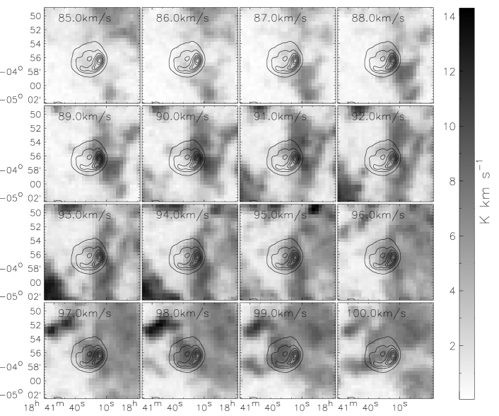
Figure 4: ${}^{12}{\rm CO}$ ($J$=1-0) intensity maps integrated over successive $1\,{\,{\rm km}\,{\rm s}^{-1}}$ intervals in the velocity range 84.5$-$100.5$\,{\,{\rm km}\,{\rm s}^{-1}}$. The velocity labeling each image is the central velocity of the interval. The contours are the same as those in Figure 3.

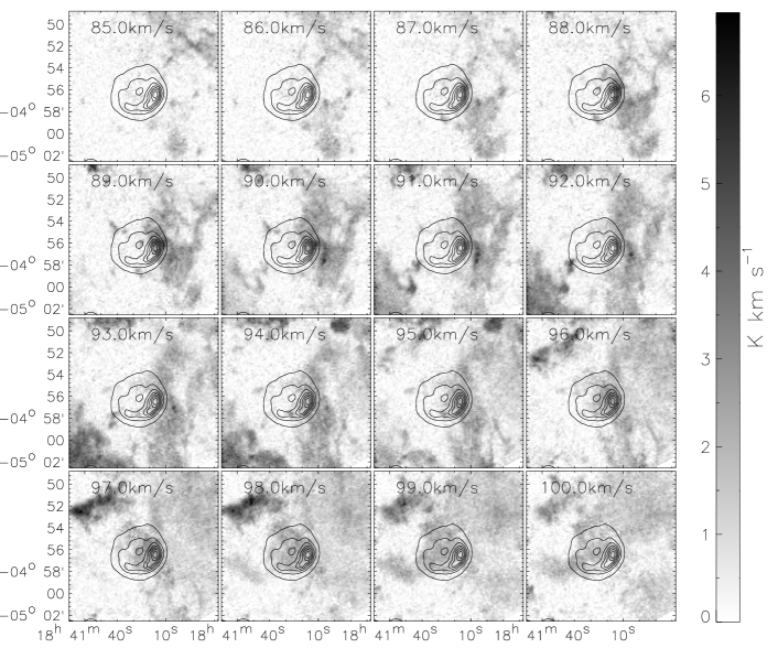
Figure 5: ${}^{12}{\rm CO}$ ($J$=3-2) intensity maps integrated over successive $1\,{\,{\rm km}\,{\rm s}^{-1}}$ intervals in the velocity range between 84.5 and $100.5\,{\,{\rm km}\,{\rm s}^{-1}}$. The velocity labeling each image is the central velocity of the interval. The contours are the same as those in Figure 3.

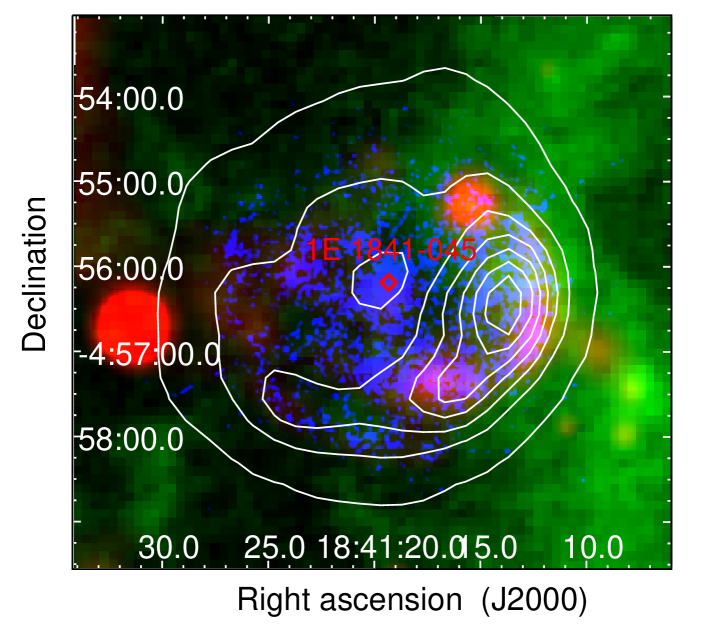
Figure 6: Tricolor image of Kes 73 for multiple wavelengths. Red: mid-IR emission at $22\,\mu{\rm m}$ (Band 4) from WISE observation. Blue: X-ray emission (2.7–7  keV) from Chandra observation (ObsID: 729). Green: ${}^{12}{\rm CO}$ ($J$=3-2) integrated intensity map in the velocity range 85–$96\,{\,{\rm km}\,{\rm s}^{-1}}$. The contours are the same as those in Figure 3.

Figure 4 and Figure 5 show the ${}^{12}{\rm CO}$ ($J$=1-0)- and ${}^{12}{\rm CO}$ ($J$=3-2)-line channel maps in the $86-100\,{\,{\rm km}\,{\rm s}^{-1}}$ velocity interval. In the interval 85–$96\,{\,{\rm km}\,{\rm s}^{-1}}$, an extended, curved MC along the north-south orientation appears to overlap the western region of the SNR Kes 73, where the radio, mid-IR and X-ray emission are brightened (also see Figure 6). This demonstrates the morphological agreement between the SNR shell and the MC.

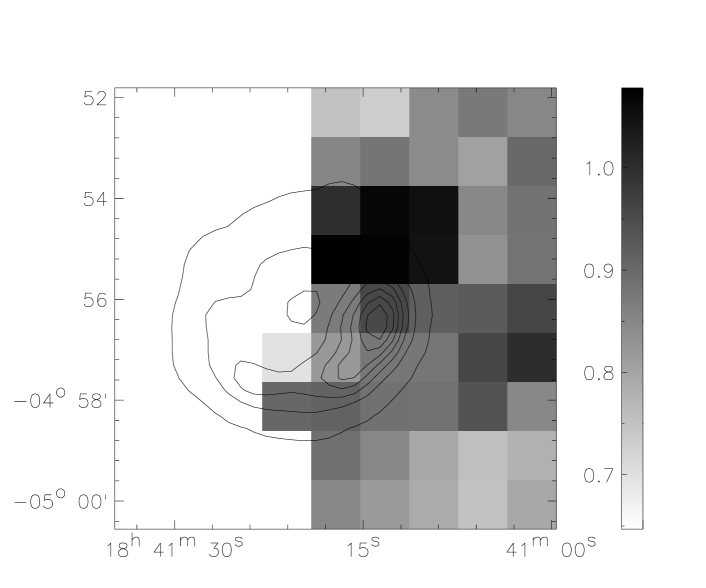
Figure 7: ${}^{12}{\rm CO}$ $J$=2-1/$J$=1-0 line ratio map for the LSR velocity range 85–$88\,{\,{\rm km}\,{\rm s}^{-1}}$. The pixels with ${}^{12}{\rm CO}$ ($J$=1-0) or ${}^{12}{\rm CO}$ ($J$=2-1) significance $<3\sigma$ are left blank. The contours are the same as those in Figure 3.

The integrated CO line emission with a high high-to-low excitation line ratio in the line wing is suggested as a probe of the SNR-MC interaction (Seta et al., 1998; Jiang et al., 2010; Chen et al., 2014). The ${}^{12}{\rm CO}$ ($J$=2-1) /${}^{12}{\rm CO}$ ($J$=1-0) ratio map in the left (blue) wing $85-88\,{\,{\rm km}\,{\rm s}^{-1}}$ is shown in Figure 7. We see along the northwestern rim the ratios are prominently elevated to $\sim 1.1$. These locations with elevated ratios may trace the relatively warm gas disturbed and heated by the SNR shock, and provide kinematic evidence for the SNR-MC interaction.

4 Discussion

4.1 The kinematic distance

It is mentioned in §3.2 that molecular components at around 18 and $90\,{\rm km}\,{\rm s}^{-1}$ appear to have morphological correspondence with the SNR. Each $V_{\scriptscriptstyle\rm LSR}$ corresponds to two (near and far) kinematic distances. Here we use the Clemens’ (1985) rotation curve of the Milky Way (Clemens, 1985) together with $R_{0}=8.0\,{\rm kpc}$ (Reid, 1993) and $V_{0}=220\,{\rm km}\,{\rm s}^{-1}$ to estimate kinematic distances of the two molecular components. $V_{\scriptscriptstyle\rm LSR}\sim 18\,{\rm km}\,{\rm s}^{-1}$ corresponds to 1.1 kpc or 13.1 kpc, but they are both outside the allowed range $7.5$–$9.4$ kpc estimated from the H i absorption data (Tian & Leahy, 2008), and thus it is very unlikely for this component of molecular gas to be associated with the SNR. $V_{\scriptscriptstyle\rm LSR}\sim 90\,{\rm km}\,{\rm s}^{-1}$ corresponds to 5.2 kpc or 9.0 kpc, and the latter falls in the allowed range. We have shown evidence in §3.2 for the physical association of the $\sim 90\,{\rm km}\,{\rm s}^{-1}$ MC with the SNR, and therefore we adopt 9.0 kpc as the distance to the MC/SNR association system.

4.2 Parameters of molecular gas

We fit the CO emissions with Gaussian lines for the $\sim 90\,{\rm km}\,{\rm s}^{-1}$ molecular gas in region “W”, and the derived parameters, molecular column density $N(\mbox{H}_{2})$, excitation temperature $T_{\rm ex}$, and optical depth of ${}^{13}{\rm CO}$ ($J$=1-0) $\tau$(${}^{13}{\rm CO}$), are summarized in Table 6. Here, the distance to the MC is taken to be 9.0  kpc. The column density of H₂ and the mass of the molecular gas are estimated using two methods. In the first method, the conversion relation for the molecular column densities, $N$(H₂) $\approx 7\times 10^{5}N$ (${}^{13}{\rm CO}$) (Frerking et al., 1982) is used under the assumption of local thermodynamic equilibrium for the molecular gas and optically thick conditions for the ${}^{12}{\rm CO}$ ($J$=1-0) line. In the second method, a value of the CO-to-H₂ mass conversion factor (the “X-factor”), $N$(H₂)/$W$(${}^{12}{\rm CO}$), $1.8\times 10^{20}$ cm^-2 K^-1 km^-1 s (Dame et al., 2001) is adopted.

4.3 The origin of $\gamma$-ray emission in the region of Kes 73

A physical association of SNR Kes 73 with the $\sim 90\,{\,{\rm km}\,{\rm s}^{-1}}$ MC can naturally explain the enhanced multiwavelength emissions along the western boundary (see Figure 6). The brightened radio emission can result from the magnetic field compression and amplification when the SNR blast wave hits the adjacent western MC and is drastically decelerated. More dust grains are swept up and heated in the west, which causes mid-IR enhancement of the western part of the shell. In a Chandra X-ray analysis of Kes 73 (Kumar et al., 2014), the western boundary (“region 1” therein) has the highest absorbing hydrogen column density and volume emission measure of the hard component that is ascribed to the forward shock. This is consistent with the encounter of the forward shock with the western dense gas (i.e., MC). The proximity of the MC on the west of the SNR is expected to play a role in the hadronic $\gamma$-ray emission from the corresponding region.

We examine the obtained $\gamma$-ray spectrum (Figure 2) by analyzing the possible leptonic and hadronic contribution to the emission from the Kes 73 region. We assume the accelerated electrons and protons have a PL distribution in energy with a high-energy cutoff $E_{i,{\rm cut}}$, namely

$$dN_{i}/dE_{i}\propto E^{-\alpha_{i}}{\rm exp}(-E_{i}/E_{i,{\rm cut}})$$ (1)

where $i=e,p$, $E_{i}$ is the particle kinetic energy, $\alpha_{i}$ is the PL index. The normalization is determined by the total energy in particles with energies above 1 GeV, $W_{i}$.

We first consider a pure leptonic model in which the $\gamma$-rays come from the relativistic electrons scattering off the seed photons, e.g., the cosmic microwave background, but find that the IC $\gamma$-rays from a single population of electrons cannot simultaneously account for the flux data at below and above 10 GeV. If only the flux measurements below 10 GeV are matched (see the green line in Figure 2a) and $\alpha_{e}=2.36$ is adopted for a consistency with the radio emission index 0.68 of the SNR (Green, 2009), the fitted parameters are $E_{e,{\rm cut}}=350$ GeV and $W_{e}=1.6\times 10^{51}d_{9}^{2}$ erg; this energy in electrons is much larger than the energy budget, a couple of tenths of the supernova explosion energy ($E_{\rm SN}\sim 10^{51}\,{\rm erg}$, canonically), which is converted to the accelerated protons and electrons.

So we add a hadronic component originating from the decay of $\pi^{0}$ mesons produced by the pp interaction between the shock-accelerated protons and the ambient gas. In this lepto-hadronic hybrid model (Model I), we set $\alpha_{e}=\alpha_{p}$ (assuming the electrons and protons are accelerated by the SNR shock), and $E_{p,{\rm cut}}=3$ PeV. The data can be fitted with parameters $\alpha_{e}=\alpha_{p}=$2.1, $E_{e,{\rm cut}}=200$ GeV, $W_{e}=$7.8$\times 10^{50}d_{9}^{2}$ erg, and $n_{t}=17(W_{p}/10^{50}\ {\rm erg})^{-1}d_{9}^{2}\,{\rm cm}^{-3}$ where $n_{t}$ is the average density (averaged over the entire shock surface) of the target protons (with which the energetic particles interact), and $W_{p}$, the energy in the accelerated protons, is assumed to be $10\%E_{\rm SN}$. In Figure 2a, the components of IC emission and pp emission dominate the flux below and above 2 GeV, respectively. In this case, however, the total energy in electrons is still unreasonably large for an SNR. Even if we consider the IR photons with energy density of $1{\rm eV\,cm}^{-3}$ and spectrum corresponding to a 40 K temperature, the energy budget of electrons $W_{e}$ would be reduced to $\sim 4.3\times 10^{50}d_{9}^{2}$ erg, which is still too high.

We then consider a pure hadronic model (Model II). As can been seen from Figure 2a, the hadronic model seems to be capable of accounting for the Fermi data, too. Also fixing the cutoff energy as $E_{p,{\rm cut}}=3$ PeV in this case, we find $\alpha_{p}=2.4$ and $n_{t}=40(W_{p}/10^{50}\ {\rm erg})^{-1}d_{9}^{2}\,{\rm cm}^{-3}$. The proton index $\alpha_{p}=2.4$ is very close to the index 2.36 of the radio-emitting electrons (derived from the radio spectral index 0.68, Green 2009), showing the consistency in the frame of the diffusive shock acceleration (DSA) theory. The proton energy budget means that if the protons accelerated by the SNR shock take up an energy $\sim 10^{50}\,{\rm erg}$, they can yield the observed $\gamma$-rays by bombarding the proximate dense gas with an average hydrogen density $n_{t}\sim 40\ {\rm cm^{-3}}$.

In Model I, an unreasonable energy in shock-accelerated electrons is obtained for the IC+pp hybrid case. The magnetar 1E 1841$-$045 seems to be a possible candidate in view of potential energy that could be released from the magnetic field decay (Takata et al., 2013; An et al., 2013). Indeed, the magnetic field decay rate ($L_{B}\gtrsim 10^{36}\,{\rm erg}\,{\rm s}^{-1}$, Yeung et al. 2017) could afford the contribution to the $\gamma$-ray emission. Therefore, we next explore whether the contribution from the magnetar can be substitute for the IC component, namely whether the $\gamma$-ray spectrum can be fitted with a combination of pp emission and emission from the magnetar (Model III). We adopt an outer gap model for isolated pulsars and AXPs (Cheng & Zhang 2001; Li et al. 2013, and specifically eq.(24) therein), in which the GeV $\gamma$-rays are the curvature radiation released by the electric field-accelerated electrons/positrons. Here the energy input is considered to be dominated by the magnetic field decay, and we assume $L_{B}=10^{36}\,{\rm erg}\,{\rm s}^{-1}$. Other model parameters are the magnetic inclination $\alpha$, the azimuthal angle $\Delta\phi$, the dimensionless parameter $\sigma_{g}$ and the solid angle of $\gamma$-ray beaming $\Delta\Omega$ (or $f_{\Omega}^{\rm th}=\Delta\Omega/4\pi$). With the parameters given in Table 5, the flux data can be fitted with the blue solid line in Figure 2b; the magnetar’s emission, represented by the long-dashed line, contributes to the flux below 10 GeV, while the pp interaction dominates the flux above 10 GeV. Like the case of pure IC emission, the magnetar emission alone cannot reproduce the Fermi $\gamma$-ray spectrum.

Next, we explore the case of Model IV, in which the flux at low energies is dominated by the magnetar, while the flux in high energies is dominated by the IC emission of the SNR shock-accelerated electrons. The electron index $\alpha_{e}$ is fixed to 2.36 again. The model curve (the black solid line in Figure 2b) appears to also be capable of matching the data points. However, the energy deposited in the accelerated electrons, $W_{e}=1.5\times 10^{50}d_{9}^{2}$ erg, is again too large to be physical.

In a short summary, the pure SNR IC emission or pure magnetar emission cannot account for the observed Fermi $\gamma$-ray spectrum. The spectral shape can be reproduced with IC+pp or IC+magnetar hybrid models (Models I and IV), but the energy in shock-accelerated electrons is unphysically large in each case. Both the pure pp hadronic interaction (Model II) and the combination of hadronic and magnetar emissions (Model III) seem to be able to account for the spectrum. They both invoke a dense adjacent gas (a few tens of H atoms cm^-3). The $\sim 90\,{\rm km}\,{\rm s}^{-1}$ cloud appears to be a suitable target of the proton bombardment. The location of the MC along the western boundary of the SNR appears to be consistent with the westward offset of the $\gamma$-ray centroid from the SNR center (§3.1.2). From Figures 3–6, we crudely estimate the subtended angle of the shock-MC interaction region as $\sim 100^{\circ}$, which corresponds to a solid angle $\Omega^{\rm had}\sim 0.7\pi$ or a fraction $f_{\Omega}^{\rm had}\sim 1/6$ of the remnant surface. We obtain an estimate for the density of the molecular gas $n({\rm H}_{2})=(1/2)n_{t}/f_{\Omega}^{\rm had}\sim 120(n_{t}/40\,{\rm cm}^{-3})\,\,{\rm cm}^{-3}$. Adopting the column density $N({\rm H}_{2})\sim 1\times 10^{22}\,{\rm cm}^{-2}$ from Table 6, the line-of-sight size of the MC is inferred to be $\sim 27(n_{t}/40\,{\rm cm}^{-3})^{-1}$ pc. But the column density given in Table 6 should be an upper limit for the associated MC because of possible contamination from other molecular gas by velocity crowding in the interval of interest as well as the potential gas at the near distance (5.2 kpc, see §4.1). Hence the line-of-sight size may be somewhat overestimated.

In Model III, the central magnetar plays an important role in the $\gamma$-ray emission from the Kes 73 region. Although the timing analysis performed by Li et al. (2017) did not detect any statistically significant $\gamma$-ray pulsation below 10 GeV being from the magnetar 1E 1841$-$045, our $\gamma$-ray spectral analysis leaves the possibility of the emission component from the magnetar.

The extension in our disk model for the $\gamma$-ray source is $0\fdg 34^{+0\fdg 06}_{-0\fdg 04}$ in radius, similar to $0\fdg 32\pm 0\fdg 03$ obtained by Li et al. (2017) and $0\fdg 32^{+0\fdg 05}_{-0\fdg 01}$ obtained by Yeung et al. (2017). As noted by Li et al. (2017), such an extension is larger than the size of SNR Kes 73. The extension is comparable to the size of the region,$45^{\prime}\times 45^{\prime}$, of our PMOD CO observation. The CO emission of the $\sim 90\,{\,{\rm km}\,{\rm s}^{-1}}$ ($85$–$96\,{\,{\rm km}\,{\rm s}^{-1}}$) MC actually pervades in the region, but the molecular gas is mainly distributed along the western boundary of the SNR (as shown in Figures 3–5). Apart from the adjacent MC and the magnetar, there may be other sources that potentially also contribute to the extended emission, such as a radio complex (Li et al., 2017) and two H ii clouds (G27.276$+$0.148 and G27.491$+$0.189, Yeung et al. 2017). Moreover, contamination from the nearby background source HESS J1841$-$055 (Aharonian et al., 2008) might be underestimated. However, given the centroid of the $\gamma$-ray emission is located on the west of the SNR, the detected Fermi GeV $\gamma$-ray emission may primarily arise from the SNR/magnetar system.

5 Summary

For the young shell-type SNR Kes 73 that harbors the central magnetar 1E 1841$-$045, we have performed an independent study of GeV $\gamma$-ray emission and carried out CO-line millimeter observations toward it. We utilized 7.6 years of Fermi-LAT observation data in a $14^{\circ}\times 14^{\circ}$ region centered on the SNR. We find an extended $\gamma$-ray source (“source A”) with the centroid on the west of the SNR, with a significance of $21.6\sigma$ in 0.1–300 GeV and an error circle of $5.^{\prime}4$ in angular radius. The $\gamma$-ray spectrum cannot be described by a pure leptonic emission (IC scattering from PL electrons with a cutoff) or a pure emission from the magnetar, and a hadronic emission component seems necessary. The CO-line observations reveal an MC at $V_{\scriptscriptstyle\rm LSR}\sim 90\,{\rm km}\,{\rm s}^{-1}$, which shows a morphological agreement with the western edge of the SNR that is brightened in multiwavelength. The ratio between ${}^{12}{\rm CO}$ $J$=2-1 and ${}^{12}{\rm CO}$ $J$=1-0 in the left (blue) wing 85–88$\,{\rm km}\,{\rm s}^{-1}$ is prominently elevated to $\sim 1.1$ in the northwestern boundary, providing kinematic evidence of the SNR-MC interaction. This SNR-MC association yields a kinematic distance of $9\,{\rm kpc}$. It is shown that the MC is an appropriate target for the p-p collision for generating the hadronic $\gamma$-ray emission component. The $\gamma$-ray spectrum can be interpreted with a pure hadronic emission or a magnetar+hadronic hybrid emission. In the case of pure hadronic emission, the spectral index of the protons 2.4 is very close to that of the radio emitting electrons, which is essentially consistent with the DSA theory. In the case of magnetar+hadronic hybrid emission, a magnetic field decay rate $\gtrsim 10^{36}\,{\rm erg}\,{\rm s}^{-1}$ is needed to power the curvature radiation of the magnetar. If leptonic emission of the SNR is considered as a component of the detected $\gamma$-rays, the electron energy budget would be unphysically high.

Table 1: The TS_ext values obtained from uniform disk model with various radii

Radius $r_{disk}$ ($\arcdeg$)	point	$0.20$	$0.22$	$0.24$	$0.26$	$0.28$
TSext	—	32.0	33.8	35.9	38.0	38.8
Radius ($\arcdeg$)	$0.30$	$0.32$	$0.34$	$0.36$	$0.38$	$0.40$
TSext	39.0	39.6	40.1	39.9	39.6	38.7

Table 2: Formulae for different spectrum types

Name	Formula/Function
PL	$\mathrm{d}N/\mathrm{d}E=N_{0}(E/E_{0})^{-\Gamma}$
PLEC	$\mathrm{d}N/\mathrm{d}E=N_{0}(E/E_{0})^{-\Gamma}\exp(-E/E_{\mathrm{cut}})$
LogP	$\mathrm{d}N/\mathrm{d}E=N_{0}(E/E_{0})^{-\Gamma-\beta\log(E/E_{0})}$
BKPL	$\mathrm{d}N/\mathrm{d}E=\begin{cases}N_{0}(E/E_{\mathrm{b}})^{-\Gamma_{1}}&\mbox{if }E<E_{\mathrm{b}}\\ N_{0}(E/E_{\mathrm{b}})^{-\Gamma_{2}}&\mbox{otherwise}\end{cases}$

Table 3: Results from spectral analysis for different spectrum types

model	$\Gamma$ or $\Gamma_{1}$	$\beta$ or $\Gamma_{2}$	$E_{\mathrm{cut}}$ or $E_{\mathrm{b}}$  (GeV)	$2\log({\mathcal{L}}_{\rm model}/{\mathcal{L}}_{\rm PL})$	${\rm TS}$
PL	2.21$\pm$0.06	—	—	—	467.5
PLEC	2.07$\pm$0.13	—	30.0$\pm$23.6	$-$4.4	420.1
LogP	1.99$\pm$0.06	0.05$\pm$0.02	0.3	6.6	434.6
BKPL	1.79$\pm$ 0.05	2.35$\pm$0.02	1.00$\pm$0.01	14.3	429.7

Table 4: Fermi LAT flux measurements of source A in the Kes 73 region

$E_{\rm ph}$ (energy band)	$E_{\rm ph}^{2}dN(E_{\rm ph})/dE_{\rm ph}$	TS
(GeV)	($10^{-12}$ erg cm-2 s-1)
0.173 (0.100–0.300)	13.9$\pm$2.1$\pm$7.1	85.1
0.548 (0.300–1.000)	14.8$\pm$1.8$\pm$4.5	249.6
1.732 (1.000–3.000)	9.0$\pm$1.0$\pm$2.4	136.2
5.477 (3.000–10.00)	4.6$\pm$0.9$\pm$0.8	40.1
17.32 (10.00–30.00)	4.3$\pm$1.1$\pm$0.3	20.4
54.77 (30.00–100.0)	$\leq 3.8$	1.2
173.2 (100.0–300.0)	$\leq 10.0$	5.2

Table 5: Model parameters

		pp		IC
Model	$\alpha_{p}$	$n_{t}$	$\alpha_{e}$	$E_{e,{\rm cut}}$	$W_{e}$
		$(W_{p}/10^{50}\ {\rm erg})^{-1}d_{9}^{2}\,{\rm cm}^{-3}$		TeV	$10^{50}$ erg
I. lepto-hadronic	2.1	17	2.1	0.2	7.8
II. hadronic	2.4	40	—	—	—
III. magnetar + hadronic	2.1	17	—	—	—
IV. magnetar + leptonic	—	—	2.36	2.5	1.5

Table 6: Fitted and Derived Parameters for the MCs Around $90\,{\rm km}\,{\rm s}^{-1}$ in Region “W”

Gaussian components
Line	Center ($\,{\rm km}\,{\rm s}^{-1}$)	FWHM ($\,{\rm km}\,{\rm s}^{-1}$)	$T_{\rm peak}$(K)	$W$(K $\,{\rm km}\,{\rm s}^{-1}$)
${}^{12}{\rm CO}$($J$=1-0)	$90.1$	5.9	8.1	50.9
${}^{13}{\rm CO}$($J$=1-0)	$89.9$	4.2	2.5	11.0
Molecular gas parameters
$N$(H2)($10^{21}$cm-2)	$M(10^{4}d_{9}^{-2}M_{\odot})$	$T_{\rm ex}$(K)	$\tau$(${}^{13}{\rm CO}$)
13.5/9.2	2.9/2.0	15.3	0.37

References

- Abdo et al. (2009) Abdo, A. A., Ackermann, M., Ajello, M., et al. 2009, ApJ, 706, L1
- Abdo et al. (2010) —. 2010, Science, 327, 1103
- Acero et al. (2015) Acero, F., Ackermann, M., Ajello, M., et al. 2015, ApJS, 218, 23
- Acero et al. (2016) —. 2016, ApJS, 224, 8
- Aharonian et al. (2008) Aharonian, F., Akhperjanian, A. G., Barres de Almeida, U., et al. 2008, A&A, 477, 353
- An et al. (2013) An, H., Hascoët, R., Kaspi, V. M., et al. 2013, ApJ, 779, 163
- Atwood et al. (2009) Atwood, W. B., Abdo, A. A., Ackermann, M., et al. 2009, ApJ, 697, 1071
- Beloborodov & Thompson (2007) Beloborodov, A. M., & Thompson, C. 2007, ApJ, 657, 967
- Borkowski & Reynolds (2017) Borkowski, K. J., & Reynolds, S. P. 2017, ApJ, 846, 13
- Chen et al. (2014) Chen, Y., Jiang, B., Zhou, P., et al. 2014, in IAU Symposium, Vol. 296, Supernova Environmental Impacts, ed. A. Ray & R. A. McCray, 170–177
- Cheng & Zhang (2001) Cheng, K. S., & Zhang, L. 2001, ApJ, 562, 918
- Clemens (1985) Clemens, D. P. 1985, ApJ, 295, 422
- Condon et al. (1998) Condon, J. J., Cotton, W. D., Greisen, E. W., et al. 1998, AJ, 115, 1693
- Dame et al. (2001) Dame, T. M., Hartmann, D., & Thaddeus, P. 2001, ApJ, 547, 792
- Dempsey et al. (2013) Dempsey, J. T., Thomas, H. S., & Currie, M. J. 2013, ApJS, 209, 8
- Frerking et al. (1982) Frerking, M. A., Langer, W. D., & Wilson, R. W. 1982, ApJ, 262, 590
- Gao et al. (2016) Gao, Z. F., Li, X.-D., Wang, N., et al. 2016, MNRAS, 456, 55
- Green et al. (1997) Green, A. J., Frail, D. A., Goss, W. M., & Otrupcek, R. 1997, AJ, 114, 2058
- Green (2009) Green, D. A. 2009, Bulletin of the Astronomical Society of India, 37, 45
- Helfand et al. (1994) Helfand, D. J., Becker, R. H., Hawkins, G., & White, R. L. 1994, ApJ, 434, 627
- Helfand et al. (1992) Helfand, D. J., Zoonematkermani, S., Becker, R. H., & White, R. L. 1992, ApJS, 80, 211
- Jiang et al. (2010) Jiang, B., Chen, Y., Wang, J., et al. 2010, ApJ, 712, 1147
- Kilpatrick et al. (2016) Kilpatrick, C. D., Bieging, J. H., & Rieke, G. H. 2016, ApJ, 816, 1
- Kumar et al. (2014) Kumar, H. S., Safi-Harb, S., Slane, P. O., & Gotthelf, E. V. 2014, ApJ, 781, 41
- Lande et al. (2012) Lande, J., Ackermann, M., Allafort, A., et al. 2012, ApJ, 756, 5
- Li et al. (2017) Li, J., Rea, N., Torres, D. F., & de Oña-Wilhelmi, E. 2017, ApJ, 835, 30
- Li et al. (2013) Li, X., Jiang, Z. J., & Zhang, L. 2013, ApJ, 765, 124
- Massaro et al. (2004) Massaro, E., Perri, M., Giommi, P., & Nesci, R. 2004, A&A, 413, 489
- Nolan et al. (2012) Nolan, P. L., Abdo, A. A., Ackermann, M., et al. 2012, ApJS, 199, 31
- Pavlovic et al. (2014) Pavlovic, M. Z., Dobardzic, A., Vukotic, B., & Urosevic, D. 2014, Serbian Astronomical Journal, 189, 25
- Reid (1993) Reid, M. J. 1993, ARA&A, 31, 345
- Seta et al. (1998) Seta, M., Hasegawa, T., Dame, T. M., et al. 1998, ApJ, 505, 286
- Shan et al. (2012) Shan, W., Yang, J., Shi, S., et al. 2012, IEEE Transactions on Terahertz Science and Technology, 2, 593
- Takata et al. (2013) Takata, J., Wang, Y., Wu, E. M. H., & Cheng, K. S. 2013, MNRAS, 431, 2645
- Tian & Leahy (2008) Tian, W. W., & Leahy, D. A. 2008, ApJ, 677, 292
- Ulich & Haas (1976) Ulich, B. L., & Haas, R. W. 1976, ApJS, 30, 247
- Vasisht & Gotthelf (1997) Vasisht, G., & Gotthelf, E. V. 1997, ApJ, 486, L129
- Verbiest et al. (2012) Verbiest, J. P. W., Weisberg, J. M., Chael, A. A., Lee, K. J., & Lorimer, D. R. 2012, ApJ, 755, 39
- Wenger et al. (2000) Wenger, M., Ochsenbein, F., Egret, D., et al. 2000, A&AS, 143, 9
- Wright et al. (2010) Wright, E. L., Eisenhardt, P. R. M., Mainzer, A. K., et al. 2010, AJ, 140, 1868
- Yeung et al. (2017) Yeung, P. K. H., Kong, A. K. H., Tam, P. H. T., et al. 2017, ApJ, 837, 69
- Zuo et al. (2011) Zuo, Y. X., Li, Y., Sun, J. X., et al. 2011, Acta Astronomica Sinica, 52, 152