Uniformly rotating, axisymmetric and triaxial quark stars in general relativity

Abstract

Quasi-equilibrium models of uniformly rotating axisymmetric and triaxial quark stars are computed in general relativistic gravity scenario. The Isenberg-Wilson-Mathews (IWM) formulation is employed and the Compact Object CALculator (cocal) code is extended to treat rotating stars with finite surface density and new equations of state (EOSs). Besides the MIT bag model for quark matter which is composed of de-confined quarks, we examine a new EOS proposed by Lai and Xu that is based on quark clustering and results in a stiff EOS that can support masses up to $3.3M_{\odot}$ in the case we considered. We perform convergence tests for our new code to evaluate the effect of finite surface density in the accuracy of our solutions and construct sequences of solutions for both small and high compactness. The onset of secular instability due to viscous dissipation is identified and possible implications are discussed. An estimate of the gravitational wave amplitude and luminosity based on quadrupole formulas is presented and comparison with neutron stars is discussed.

I Introduction

The recent gravitational-wave (GW) event GW170817 together with accompanying electromagnetic emission observations The LIGO Scientific Collaboration and The Virgo Collaboration (2017); The LIGO Scientific Collaboration et al. (2017a) from a binary neutron star (BNS) merger has opened a brand new multi-messenger observation era for us to explore the Universe. Apart from enriching our knowledge on origins of short gamma-ray bursts LIGO Scientific Collaboration et al. (2017) and nucleosynthesis associated with BNS mergers The LIGO Scientific Collaboration et al. (2017b); Baiotti and Rezzolla (2017), it also provides an effective way for us to constrain the equation of state (EOS) of neutron stars (NS). In addition to systems such as binary black-hole mergers and BNS mergers, rapidly rotating compact stars have also been considered as important candidates of GW sources Andersson et al. (2011), which could be detected by ground-based GW observatories Abramovici et al. (1992); Punturo et al. (2010); Accadia et al. (2011); Kuroda and LCGT Collaboration (2010); Aso et al. (2013) and help us understand the nature of strong interaction of dense matter.

It has been long since the equilibrium models of self-gravitating, uniformly rotating, incompressible fluid stars were systematically studied in a Newtonian gravity scheme Chandrasekhar (1969). Depending on the rotational kinetic energy, the configuration could be axisymmetric Maclaurin ellipsoids as well as nonaxisymmetric ellipsoids, such as Jacobian (triaxial) ellipsoid. For compact stars that we are interested in for GW astronomy, however, general relativity is required to replace Newtonian gravity. The field of relativistic rotating stars has been studied for many years Meinel et al. (2008); Friedman and Stergioulas (2013).

A rotating NS will spontaneously break its axial symmetry if the rotational kinetic energy to gravitational binding energy ratio, $T/|W|$ exceeds a critical value. This instability can either be of secular type Shapiro and Zane (1998); Bonazzola et al. (1996); Gondek-Rosińska and Gourgoulhon (2002); Bonazzola et al. (1998) or dynamical Houser and Centrella (1996); Pickett et al. (1996); Brown (2000); New et al. (2000); Liu (2002); Watts et al. (2005); Baiotti et al. (2007); Manca et al. (2007); Corvino et al. (2010), depending on the process driving the instability and with only small modifications if a magnetisation is present Camarda et al. (2009); Franci et al. (2013); Muhlberger et al. (2014) (see Andersson (2003) for a review). A high $T/|W|$ ratio can also be reached for a newly born rotating compact star during a core collapse supernova or for a NS which is spun up by accretion Lai and Shapiro (1995); Bildsten (1998); Woosley and Janka (2005); Watts et al. (2008); Piro and Thrane (2012).

Quasi-equilibrium figures of triaxially rotating NSs have also been created and studied in full general relativity Huang et al. (2008); Uryū et al. (2016). In this case, the bifurcation from an axisymmetric to triaxial configuration happens very close to the mass shedding limit, and, for soft NS EOSs or for NSs with large compactness, the triaxial sequence could totally vanish James (1964); Bonazzola et al. (1996, 1998); Hachisu and Eriguchi (1982); Lai et al. (1993). As a result, it is presently unclear whether triaxial configurations of NSs can actually be realized in practice.

On the other hand, it is worth noting that the EOS of compact stars is still a matter of lively debate since astronomical observations are not sufficient to rule out many of the nuclear-physics EOSs that are compatible with the observations. As a result, besides the popular idea of NSs, other models for compact stars are possible and have been considered in the past. A particularly well developed literature is the one concerned with strange quark stars (QSs), since it was long conjectured that strange quark matter composed of de-confined up, down and strange quarks could be absolutely stable Bodmer (1971); Witten (1984). There is also possible observational evidence indicating the existence of QSs (for a recent example, see Dai et al. (2016)). Additionally, the small tidal deformability of QSs is favoured by the observation of GW170817 Lai et al. (2017) and possible models with QS merger or QS formations are also suggested to explain the electromagnetic counterparts for a short gamma-ray burst (c.f. Li et al. (2016); Lai et al. (2017)).

Following this possibility, a large effort has been developed to calculate equilibrium configurations of QSs, starting from the first attempts Itoh (1970); Alcock et al. (1986); Haensel et al. (1986). At present, both uniformly rotating Gondek-Rosińska et al. (2000); Gourgoulhon et al. (1999); Stergioulas et al. (1999) and differentially rotating QSs Szkudlarek et al. (2012) have been studied in full general relativity. Unlike NSs, which are bound by self-gravity, QSs are self-bound by strong interaction. Consequently, rotating QSs can reach a much larger $T/|W|$ ratio compared with NSs and the triaxial instability could play a more important role Gondek-Rosinska et al. (2000); Gondek-Rosińska et al. (2000, 2001). The triaxial bar mode (Jacobi-like) instability for MIT bag-model EOS has been investigated in a general relativistic framework Gondek-Rosińska et al. (2003).

We here use the Compact Object CALculator code, cocal, to build general-relativistic triaxial QS solution sequences using different EOS models. cocal is a code to calculate general-relativistic equilibrium and quasi-equilibrium solutions for binary compact stars (black hole and NS) as well as rotating (uniformly or differentially) NSs Uryū and Tsokaros (2012); Uryū et al. (2012); Tsokaros and Uryū (2012); Tsokaros et al. (2015); Huang et al. (2008); Uryū et al. (2016). The part of the cocal code handling the calculation of the EOS was originally designed for piecewise polytropic EOSs. We have here extended the code to include polynomial type of EOSs, as those that can be used to describe QSs. In doing so the trivial relationship between the thermodynamic quantities for a piecewise polytrope (e.g., see Eqs. (64)–(68) in Tsokaros et al. (2015)), is lost and now one has to apply root finding methods. Another issue is related to the surface fitted coordinates that are used in cocal to track the surface of the star. For NSs, the surface was identified as the place where the rest-mass density goes to zero or where the specific enthalpy becomes one. This is no longer generally true for a self-bound QS and a different approach needs to be developed. The nonlinear algebraic system that determines the angular velocity, the constant from the Euler equation, and the renormalization constant of the spherical grid has to be modified in order to accommodate the arbitrary surface enthalpy.

We here compute solutions for both axisymmetric and triaxial rotating QSs with the new code, as well as sequences with various QS EOS and different compactnesses. We checked our new implementation for those cases were previous studies have been possible Huang et al. (2008), and we confirm the accuracy of our new code. We discuss the astrophysical implications of the quantities of rotating QSs at the bifurcation point. For instance, the spin frequency at the bifurcation point could be a more realistic spin up limit for compact stars rather than the mass shedding limit, which relates to the fastest spinning pulsar we might be able to observe. The GW strain and luminosity estimates for our models are given, while full numerical simulations are left for the future (see Tsokaros et al. (2017) for recent simulations involving triaxial NSs).

The structure of this paper is organized as follows: In Sec. II we discuss the formulation we used and the field equations (Sec. II.1), the hydrodynamics (Sec. II.2) and the EOS part (Sec. II.3). In order to test the behavior of the modified code, we have performed convergence tests with five resolutions and compared with rotating NS solutions built by the original cocal code. These tests can be found in Sec. III. Triaxially deformed rotating QS sequences for different compactnesses, are presented in Sec. IV, while the implications for the astrophysical observations of this work are presented in Sec. VI. Hereafter we use units with $G=c=M_{\odot}=1$ unless otherwise stated; a conversion table to the standard cgs units can be found, for instance, in Rezzolla and Zanotti (2013).

II Formulation and numerical method

II.1 Field equations

In order to solve the field equations numerically, the Isenberg-Wilson-Mathews (IWM) formulation Isenberg and Nester (1980); Isenberg (2008); Wilson and Mathews (1989) is employed. In a coordinate chart $\{t,x^{i}\}$, the $\mathrm{3+1}$ decomposition of the spacetime metric gives

$$ds^{2}=-\alpha^{2}dt^{2}+\psi^{4}\delta_{ij}(dx^{i}+\beta^{i}dt)(dx^{j}+\beta^{j}dt)\,,$$ (1)

where $\alpha,\ \beta^{i}$ are the lapse and shift vector (the kinematical quantities), while $\gamma_{ij}=\psi^{4}\delta_{ij}$ is the IWM approximation for the three-metric.

The extrinsic curvature of the foliation is defined by

$$K_{ab}\,:=\,-\frac{1}{2\alpha}\partial_{t}\gamma_{ab}+\frac{1}{2\alpha}\mbox{\pounds}_{\beta}\gamma_{ab}\,.$$ (2)

and a maximal slicing condition $K=0$ is assumed.

Decomposing the Einstein equations with respect to the normal $n^{\alpha}$ of foliation, we get the following 5 equations in terms of the five metric coefficients $\{\psi,\beta^{a},\alpha\}$ on the initial slice $\Sigma_{0}$:

$$(G_{\alpha\beta}-8\pi T_{\alpha\beta})\,n^{\alpha}n^{\beta}\ \,=\,0,$$ (3)

$$(G_{\alpha\beta}-8\pi T_{\alpha\beta})\,\gamma^{i\alpha}n^{\beta}\,=\,0,$$ (4)

$$(G_{\alpha\beta}-8\pi T_{\alpha\beta})\,\Big{(}\gamma^{{\alpha\beta}}+\frac{1}{2}n^{\alpha}n^{\beta}\Big{)}\,=\,0,$$ (5)

where the first and second equations are the Hamiltonian and momentum constraints, respectively. Here $\gamma_{\alpha\beta}=g_{\alpha\beta}+n_{\alpha}n_{\beta}$ is the projection tensor onto the spatial slices. These equations can be written in the form of elliptic equations with the non-linear source terms, respectively,

$$\!\!\!\!\!\!\!\nabla^{2}\psi\,=\,-\frac{\psi^{5}}{8}A_{ab}A^{ab}-2\pi\psi^{5}\rho_{\rm H},$$ (6)

$$\!\!\!\!\!\!\!\nabla^{2}\beta^{a}+\frac{1}{3}\partial^{a}\partial_{b}\beta^{b}\,=\,-2\alpha A^{ab}\partial_{b}\ln\frac{\psi^{6}}{\alpha}+16\pi\alpha j^{a},$$ (7)

$$\!\!\!\!\!\!\!\nabla^{2}(\alpha\psi)\,=\,\frac{7}{8}\alpha\psi^{5}A_{ab}A^{ab}+2\pi\alpha\psi^{5}(\rho_{\rm H}+2S).$$ (8)

where $A^{ij}=K^{ij}={\psi^{-4}}(\partial^{i}\beta^{j}+\partial^{j}\beta^{i}-\frac{2}{3}\delta^{ij}\partial_{k}\beta^{k})/{2\alpha}$, and the source terms of matter are defined by $\rho_{\rm H}:=T_{\alpha\beta}n^{\alpha}n^{\beta}$, $j^{i}:=-T_{\alpha\beta}\gamma^{i\alpha}n^{\beta}$, and $S:=T_{\alpha\beta}\gamma^{\alpha\beta}$.

The above set of equations must be supplied with boundary conditions at infinity. Since we are working in the inertial frame and we impose asymptotic flatness, we must have

$$\lim_{r\rightarrow\infty}\psi=1\,,\qquad\lim_{r\rightarrow\infty}\alpha=1\,,\qquad\lim_{r\rightarrow\infty}\beta^{i}=0\,.$$ (9)

II.2 Hydrostatic equilibrium

The hydrostatic equation for a perfect fluid in quasi-equilibrium can be derived from the relativistic Euler equation Rezzolla and Zanotti (2013)

$$u^{\beta}\nabla_{\beta}(hu_{\alpha})+\nabla_{\alpha}h\,=0\,,$$ (10)

where $u^{\alpha}=u^{t}(1,v^{i})=u^{t}(1,\Omega\phi^{i})$ is the 4-velocity of the fluid, $\phi^{i}=(-y,x,0)$, and $h$ is the specific enthalpy defined by $h:=(\epsilon+p)/\rho$ ($\rho$ is the rest-mass density and $\epsilon$ the total energy density).

When the symmetry along a helical Killing vector $k^{\alpha}=t^{\alpha}+\Omega\phi^{\alpha}$ is imposed for the fluid variables, which is approximately true also in the case for a rotating nonaxisymmetric star in quasi-equilibrium, the integral of the Euler equation becomes

$$\frac{h}{u^{t}}\,=\,\mathcal{E}\,,$$ (11)

where $\mathcal{E}$ is a constant. From the normalization of the four velocity $u_{\alpha}u^{\alpha}=-1$, one obtains

$$u^{t}=\frac{1}{\sqrt{\alpha^{2}-\omega_{a}\omega^{a}}}=\frac{1}{\sqrt{\alpha^{2}-\psi^{4}\delta_{ab}\,\omega^{a}\omega^{b}}}\,,$$ (12)

where $\omega^{a}=\beta^{a}+\Omega\phi^{a}$. The fluid sources of Eqs. (6)–8, i.e., $\rho_{\mathrm{H}}$, $j_{a}$ and $S$, are defined in terms of the energy momentum tensor in the previous section. In terms of the fluid and field variables they can be written as Rezzolla and Zanotti (2013)

$$\rho_{\mathrm{H}}=\rho[h(\alpha u^{t})^{2}-q],$$ (13)

$$j^{i}=\rho h\alpha(u^{t})^{2}\gamma^{i\alpha}u_{\alpha},$$ (14)

$$S=\rho h(\alpha u^{t})^{2}-\rho h+3\rho q,$$ (15)

in which $q:=p/\rho$ is the relativistic analogue of the Emden function. Here $u^{t}$ is related to $h$ through Eq. (11). Therefore in order to close the system, an additional relationship is needed between the specific enthalpy, the pressure and the rest-mass density of the fluid, i.e., an EOS. Once such a relation is available, to solve the field equations [Eqs. (6)–8] and the hydrostatic equation [Eq. (11)] one has to find the two constants $\{\Omega,\mathcal{E}\}$ that appear in all of them. This procedure is described in detail for example in Ref. Tsokaros et al. (2015).

II.3 Equation of State

In this work, we have considered two types of EOS for QSs. One of them is the MIT bag-model EOS Chodos et al. (1974), since it is the most widely used EOS for QSs. In the case when strange quark mass is neglected, the pressure is related to total energy density according to

$$p=\sigma(\epsilon-\epsilon_{s})\,,$$ (16)

where $\sigma,\ \epsilon_{s}$ are two constants, the second being the total energy density at the surface. Related to $\epsilon_{s}$ is the so called bag constant, $B=\epsilon_{s}/4$. In this work, and following Limousin et al. (2005), the simplest MIT bag-model EOS has been employed, where $\sigma=1/3$ and $B^{1/4}=138\,\mathrm{MeV}$.

Besides the MIT bag-model EOS, we have also considered another QS EOS suggested by Lai and Xu Lai and Xu (2009), which we will refer to as the LX EOS hereafter. Unlike the conventional QS models (e.g., the MIT bag-model EOS) which are composed of de-confined quarks, Lai and Xu Lai and Xu (2009) suggested that quark clustering is possible at the density of a cold compact star since the coupling of strong interaction is still decent at such energy scale. Due to the non-perturbative effect of strong interaction at low energy scales and the many-body problem, it is very difficult to derive the EOS of such a quark-cluster star from first principles.

Lai and Xu attempted to approach the EOS of such quark-cluster star with phenomenological models, i.e., to compare the intercluster potential with the interaction between inert molecules (a similar approach has also been discussed in Guo et al. (2014)). They also take the lattice effects into account as the potential could be deep enough to trap the quark clusters. Combining the inter-cluster potential and the lattice thermodynamics, they have derived an EOS in the following form:

$$p=4U_{0}(12.4r_{0}^{12}n^{5}-8.4r_{0}^{6}n^{3})+\frac{1}{8}(6\pi^{2})^{\frac{1}{3}}\hbar cn^{\frac{4}{3}}\,,$$ (17)

where $\hbar$ is the reduced Planck constant. The parameters in this expression, $U_{0}$ and $r_{0}$, are the depth of the potential and characteristic range of the interaction, respectively. The EOS is also dependent on the number of quarks in each cluster ($N_{\mathrm{q}}$) since it relates the energy density ($\epsilon$) and rest-mass density ($\rho$) to the number-density of quark clusters ($n$ in Eq. (17)). Similarly to the MIT bag-model EOS case, we use the rest-mass density parameter, which is

$$\rho=m_{\mathrm{u}}\frac{N_{\mathrm{q}}}{3}n\,,$$ (18)

where $m_{\mathrm{u}}=931\mathrm{MeV}/c^{2}$ is the atomic mass unit. While several different choices of parameters are considered in Ref. Lai and Xu (2009), in our work we restrict our attention to $U_{0}=50\,\mathrm{MeV}$ and for $N_{\mathrm{q}}=18$. We also note that although it is not as obvious as for the MIT bag-model EOS, the LX EOS also has a nonzero surface density since expression Eq. (17) has a unique zero root when the number density is positive.

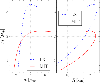
Figure 1: The TOV solution sequences for MIT bag-model EOS (red solid line) and the LX EOS (blue dashed line) respectively. The left panel shows the mass-central density relationship for each model and the right panel is the mass-radius diagram. The bag constant we apply in this work for the MIT bag-model EOS satisfies the 2 solar mass constraint from observations.

Being a stiff EOS, the LX EOS is favored by the discovery of massive pulsars Lai and Xu (2011); Demorest et al. (2010); Antoniadis et al. (2013). The rest-mass density and mass-radius relationships for spherical models can be seen in Fig. 1, and the characteristics of the maximum mass models are reported in Table 2. The LX EOS has also been discussed in relation with the possibility of understanding some puzzling observations related to compact stars, such as the energy release during pulsar glitches Zhou et al. (2014), the peculiar X-ray flares Xu and Liang (2009) and the optical/UV excess of X-ray-dim isolated NSs Wang et al. (2017). Particularly, a solid QS model has been suggested in order to understand those observations Xu (2003). However, as pointed out in Zhou et al. (2014), the critical strain of such a star is very small. A starquake will be induced when the relative difference in ellipticity is $10^{-6}$, for most, between the actual configuration of the star and the configuration as if the star is a perfect fluid. This is consistent with the pulsar glitch observations on Vela. Therefore, we find it a good approximation to calculate the quasi-equilibrium configuration of such a star with perfect fluid assumption.

Understanding the models and properties of the QS EOSs that we want to consider, we can modify the EOS part of the simulation code, which was originally designed for NS models, accordingly.

As mentioned above, in the case of NSs, a piecewise-polytropic EOS is usually assumed to describe the EOS Read et al. (2009); Rezzolla and Zanotti (2013). In each piece, the pressure and rest-mass density are related as

$$p_{i}=\kappa_{i}\rho^{\Gamma_{i}}=\kappa_{i}\rho^{1+1/n_{i}}\,,\qquad i=1,2,\ldots,N\,.$$ (19)

For QSs, due to the nonzero surface density and nonzero energy density integration constant, we will assume that the EOS is generally a polynomial

$$p=\sum\limits_{i=1}^{N}\kappa_{i}\rho^{\Gamma_{i}}\,.$$ (20)

Given the relationship between $p$ and $\rho$, one can apply the first law of thermodynamics to obtain other quantities such as the energy density and the specific enthalpy. In the zero-temperature case, the first law of thermodynamics can be expressed as Rezzolla and Zanotti (2013)

$$d\epsilon=\frac{\epsilon+p}{\rho}d\rho,\quad\mbox{or}\quad d\left(\frac{\epsilon}{\rho}\right)=\frac{p}{\rho^{2}}d\rho\,,$$ (21)

which can be integrated to obtain the total energy density. The integral constant is usually chosen to be 1, since when there is no internal energy, the energy density and the rest-mass density coincide (apart from the square of the speed of light). However, for QS EOSs (like in Guo et al. (2014) and the MIT bag-model EOS), the integral constant is different from unity and needs to be properly taken into account.

MIT bag-model EOS
$C=-c^{2}$	$\rho_{s}=1.4\rho_{\mathrm{nuc}}$	$h_{s}=0.89697478c^{2}$
$N=2$	$\kappa_{i}$	$\Gamma_{i}$
$i=1$	$2.7977907\times 10^{15}$	$\frac{4}{3}$
$i=2$	$-7.5279768\times 10^{34}$	$0$
LX EOS
$C=0$	$\rho_{s}=2.0\rho_{\mathrm{nuc}}$	$h_{s}=0.96828675c^{2}$
$N=3$	$\kappa_{i}$	$\Gamma_{i}$
$i=1$	$2.0824706\times 10^{-39}$	$5$
$i=2$	$-6.1559375\times 10^{-10}$	$3$
$i=3$	$7.1307226\times 10^{13}$	$\frac{4}{3}$

Table 1: Quark EOS parameters in cgs units for MIT and the LX EOSs respectively. $\rho_{\mathrm{nuc}}$ is the nuclear saturation density which is chosen to be $2.67\times 10^{14}\,\mathrm{g\,cm^{-3}}$. Unlike NSs which have a surface enthalpy $h_{s}=1$, for QSs this value is an input parameter for a specific model. In practice one inputs the rest-mass density at the surface $\rho_{s}$ and then $h_{s}$ is computed from the EOS. The constant $C$ is the integration constant of the first law and determines the limit of the thermodynamic variables at the surface of the star.

In this case, the energy density and specific enthalpy are related to the rest-mass density by

$$\epsilon=\sum\limits_{i=1}^{N}\frac{\kappa_{i}}{\Gamma_{i}-1}\rho^{\Gamma_{i}}+\rho(1+C)\,,$$ (22)

$$h=\frac{\epsilon+p}{\rho}=\sum\limits_{i=1}^{N}\frac{\Gamma_{i}\kappa_{i}}{\Gamma_{i}-1}\rho^{\Gamma_{i}-1}+1+C\,.$$ (23)

Here $C$ is the integral constant we mentioned above. It is usually taken to be zero for NS models. Here it is introduced again in order to accommodate stars that have different surface limit for the thermodynamic variables.

The nonzero surface density of QSs requires a different boundary condition in our simulation. For typical NSs when we adjust the position of the surface, we are actually locating the points where the specific enthalpy is $1$. For QSs, the surface identification will be at values of the specific enthalpy different from unity and consistent with Eq. (23). What we typically use as input parameter is the surface rest-mass density $\rho_{s}$, from which we then calculate $h_{s}$ using Eq. (23).

As an example, for MIT bag-model EOS the first law at zero temperature implies

$$\epsilon = \frac{1}{1+\sigma}\left(\bar{C}\rho^{1+\sigma}+\sigma\epsilon_{s}\right),$$ (24)

$$p = \frac{\sigma}{1+\sigma}\left(\bar{C}\rho^{1+\sigma}-\epsilon_{s}\right),$$ (25)

$$h = \bar{C}\rho^{\sigma},$$ (26)

where $\bar{C}$ is a constant of integration. The above EOS is of the form (20) with

$$\kappa_{1}=\frac{\sigma\bar{C}}{1+\sigma},\quad\Gamma_{1}=1+\sigma,\quad\kappa_{2}=-\frac{\sigma\epsilon_{s}}{1+\sigma},\quad\Gamma_{2}=0\,,$$ (27)

and $C=-1$. Having all thermodynamical variables in terms of the rest-mass density is convenient from the computational point of view since this is one of the fundamental variables used in the cocal code, therefore the modifications with respect to the EOS will be minimal.

Given a fixed choice of $\sigma$ and $B$ for the MIT bag-model EOS, one can obtain a unique solution of the field equations under hydrostatic equilibrium (see Secs. II.1 and II.2). In other words, the relationship between the gravitational mass versus the central energy density, the mass-radius relationship and the spacetime metric will not depend on the coefficient $\bar{C}$, as it is eliminated out from Eq. (16) (similar argument can be found in Li et al. (2017); Bhattacharyya et al. (2016)). At the same time, it will indeed affect the rest mass hence the binding energy of the QS since it relates the rest-mass density and the number density of the components. Hence a reasonable choice for $\bar{C}$ will still be helpful although it will not affect anything that we are interested in for this work. Here we chose $\bar{C}$ such that the EOS corresponds to the $a_{4}=0.8$ model as in Alford et al. (2005) and we assume a rest mass of $931\,{\rm MeV}/c^{2}$ for each baryon number ($n_{b}=n_{q}/3$, where $n_{q}$ is the number density of quarks). Any other choices for $\bar{C}$ are in principle possible and they will not affect our solution except for the rest mass of the star. Actual values of these constants can be found in Table 1 in cgs units.

In Eqs. (24) and (25) we have employed the relationship which is quite similar to the explicit form of MIT bag model. By factoring out the rest mass, those two equations can be rewritten as a function of number density instead of rest-mass density. However, one clarification we want to discuss at this point is that, the choice of using Eq. (24) and (25) is not essential. Moreover, Eqs. (24) and (25) are related by the first law of thermodynamics [see Eq. (21)], which is not essential as well. We can describe the MIT EOS Eq. (16), in a parametric form $(p(\rho),\epsilon(\rho))$ with an arbitrary parameter $\rho$, as long as the functions $p(\rho)$ and $\epsilon(\rho)$ satisfy Eq. (16). In doing so we choose to satisfy Eq. (21) and therefore arrive at Eq. (24), (25). As one can see from Eqs. (13)–(15), the fluid terms that appear are $q\rho=p$ and $h\rho=\epsilon+p$. Thus, for the MIT bag-model EOS, the only thermodynamic variable that appears in the field equations is $\epsilon$. Every model thus calculated will be uniquely defined by a deformation parameter and the central total energy density. The scaling constant which is analogous to scaling as $\kappa^{n/2}$ for NSs Rezzolla and Zanotti (2013), is here $\epsilon_{s}^{-1/2}$.

EOS	$(p/\rho)_{c}$	$\epsilon_{c}$	$\rho_{c}$	$M$	$\mathcal{C}$
MIT	0.2940	$2.609\times 10^{-3}$	$2.342\times 10^{-3}$	2.217	0.2706
LX	2.326	$2.451\times 10^{-3}$	$1.744\times 10^{-3}$	3.325	0.3956

Table 2: Pressure, energy density, rest-mass density, gravitational mass, and compactness at the maximum mass of spherical solutions for the two EOSs in this work.

Before concluding this discussion on the EOSs we should mention that although a polynomial-type EOS is implemented for the calculation of QSs with a finite surface density, the developments in the new version of cocal allow us to calculate any compact star with an EOS that can be described by a polynomial function, including NSs and hybrid stars. For instance, some phenomenological approaches suggested recently in Ref. Baym et al. (2017) also result in a polynomial-type EOS, which can be computed straightforwardly with the new code.

III Code tests

The working properties of the cocal code for single rotating stars is presented in detail in previous works, e.g., Huang et al. (2008); Uryū et al. (2016), so that here we will only mention the most important quantities that are used in our simulations. The method has its origins in the works of Ostriker and Marck Ostriker and Mark (1968), who used it to compute Newtonian stars, and the works of Komatsu, Eriguchi, and Hachisu Komatsu et al. (1989), who devised a stable numerical algorithm and obtained first axisymmetric general relativistic rotating stars. From this latest work the method is commonly referred as the KEH method and consists of an integral representation of the Poisson equation commonly referred as the representation formula. Since we have only one computational domain with trivial boundary conditions at infinity, the Green’s function is $G(x,x^{\prime})=1/|x-x^{\prime}|$ and is expanded as a series of the associated Legendre polynomials and trigonometric functions. The maximum number of the terms included in this expansion is given as $L$ in Table 3.

This approach is used to compute the gravitational fields $\{\alpha,\psi,\beta^{i}\}$ while hydrostatic equilibrium is achieved through Eq. (11). At every step in the iteration to reach the solution at the desired accuracy, three constants need to be computed. The first one is the angular velocity of the star, $\Omega$, while the second one is the constant from the Euler integral, $\mathcal{E}$, in Eq. (11), and, finally, the third constant is $R_{0}$, a normalization factor for the whole domain where the equations are solved. At every step during the iteration the nonlinear equation with respect to these three constants is solved typically by evaluating Eq. (11) at three points in the star. For axisymmetric configurations, we use the center of the star and two points on the surface, one on the positive $x$-axis and one at the North pole of the stellar model. An axisymmetric equilibrium is achieved by setting the ratio between the polar axis over the equatorial radius along the $x$-axis. For triaxial configurations, on the other hand, the three points are the center of the star together with two points again on the surface, one at the positive $x$-axis, and one on the positive $y$-axis. Each triaxial solution has a fixed ratio of the radius on the $y$-axis over the radius of the $x$-axis.

From a numerical point of view, cocal is a finite-difference code that uses spherical coordinates $(r,\theta,\phi)\in[0,r_{b}]\times[0,\pi]\times[0,2\pi]$ and the basic parameters are summarized in Table 3. In the angular directions $\theta,\phi$ the discretization is uniform, i.e., $\Delta\theta=\pi/N_{\theta}$, and $\Delta_{\phi}=2\pi/N_{\phi}$. In the radial direction the grid is uniform until point $r_{c}$ with $\Delta r_{i}=r_{c}/{N_{r}^{\rm m}}$, and in the interval $[r_{c},r_{b}]$ the radial grid in non-uniform and follows a geometric series law Huang et al. (2008). While field variables are evaluated at the gridpoints, source terms under the integrals are evaluated at midpoints between two successive gridpoints since the corresponding integrals use the midpoint rule. For integrations in $r$ and $\phi$ we use a second-order midpoint rule. For integrations in $\theta$ we use a fourth-order midpoint rule. This was proven necessary to keep second order convergence at the region of maximum field strength Uryū et al. (2012). Derivatives at midpoints are calculated using second-order rule for the angular variables $\theta,\phi$, and third-order order rule for the radial variable $r$ (again for keeping second-order convergence at same regions Uryū and Tsokaros (2012)). Derivatives evaluated at gridpoints always use a fourth-order formula in all variables.

$r_{a}$	:	Radial coordinate where the grid $r_{i}$ starts.
$r_{b}$	:	Radial coordinate where the grid $r_{i}$ ends.
$r_{c}$	:	Radial coordinate between $r_{a}$ and $r_{b}$ where the
		grid changes from equidistant to non-equidistant.
$N_{r}$	:	Total number of intervals $\Delta r_{i}$ between $r_{a}$ and $r_{b}$.
${N_{r}^{\rm m}}$	:	Number of intervals $\Delta r_{i}$ in $[0,r_{c}]$.
${N_{r}^{\rm f}}$	:	Number of intervals $\Delta r_{i}$ in $[0,R(\theta,\phi)]$.
$N_{\theta}$	:	Total number of intervals $\Delta\theta_{i}$ for $\theta\in[0,\pi]$.
$N_{\phi}$	:	Total number of intervals $\Delta\phi_{i}$ for $\phi\in[0,2\pi]$.
$L$	:	Number of multipole in the Legendre expansion.

Table 3: Summary of parameters used for rotating star configurations.

Type	$r_{a}$	$r_{b}$	$r_{c}$	$N_{r}$	${N_{r}^{\rm m}}$	${N_{r}^{\rm f}}$	$N_{\theta}$	$N_{\phi}$	$L$
H2.0	0	$10^{6}$	1.25	192	80	64	48	48	12
H2.5	0	$10^{6}$	1.25	288	120	96	72	72	12
H3.0	0	$10^{6}$	1.25	384	160	128	96	96	12
H3.5	0	$10^{6}$	1.25	576	240	192	144	144	12
H4.0	0	$10^{6}$	1.25	768	320	256	192	192	12

Table 4: Five different resolutions used for convergence tests. Parameters are shown in Table 3. The number of points that covers the largest star radius is ${N_{r}^{\rm f}}$.

It is worth noting that, since for QSs the relationship between the specific enthalpy and the rest-mass density follows a general polynomial function [cf., Eq. (23)], a root-finding method needs to be employed when calculating the thermodynamical quantities from the enthalpy. The regular polynomial expression of the specific enthalpy with respect to rest-mass density allows us to use a Newton-Raphson method as the derivative can also be expressed easily. In view of this, the computational costs with a QS EOS are not significantly larger than those with NS EOS. However, in order to guarantee a solution of rest-mass density when the specific enthalpy is given, a bi-section root-finding method needs to be employed if the Newton-Raphson method does not converge sufficiently rapidly. In this case, the initial range of the bi-section method is set to be the specific enthalpy corresponding to the rest-mass densities at the stellar center and at the surface, respectively.

In previous works Huang et al. (2008); Uryū et al. (2012, 2016); Tsokaros et al. (2016), the cocal code has been extensively tested, both with respect to its convergence properties, as well as with respect in actual evolutions with other well established codes Tsokaros et al. (2016).

In what follows we report the convergence tests we have performed in order to investigate the properties of the code under these new conditions. Before doing that, we note that special care is needed when using a root-finding method to calculate thermodynamical quantities for a given specific enthalpy in the case of rotating QSs. In particular, it is crucial to consider what is the accuracy set during the root-finding step. Of course, it is possible to require that the accuracy in the root-finding step is much higher than the other convergence criteria in the code to guarantee an accurate result. In this way, however, the computational costs will increase considerably, since the thermodynamical quantities need to be calculated at every gridpoint and at every iteration. We found that an accuracy of $10^{-10}$ for the thermodynamic variables solutions neither compromises the accuracy of the solutions, nor slows down the code significantly.

III.1 Comparison with rotating NSs

Although the newly developed code presented here is intended for QS EOSs, it can be also used to produce rotating NSs if one restricts the EOS to a single polytrope. This can be accomplished by setting the polynomial terms to be only one, the surface rest-mass density $\rho_{s}=0$ and the energy integral constant $C=0$. In this case, Eq. (20) becomes

$$p=\kappa\rho^{\Gamma}=\kappa\rho^{1+1/n}\,,$$ (28)

and the relationship between the energy density, the specific enthalpy and the rest-mass density [Eqs. (22) and 23] will be exactly the same as that for a polytropic NS.

We choose a stiff EOS with $n=0.3$ and produce axisymmetric solution sequences for small and high compactness $\mathcal{C}:=M_{\rm ADM}/R=0.1,0.2$, and $M_{\rm ADM}$ is the corresponding Arnowitt-Deser-Misner (ADM) mass for a nonrotating model, both with the original rotating-NS and the modified rotating-QS solver. The grid-structure parameters used are $N_{r}=240$, ${N_{r}^{\rm m}}=80$, ${N_{r}^{\rm f}}=64$, $N_{\theta}=96$, $N_{\phi}=192$, $L=12$, $r_{b}=10^{4}$, and $r_{c}=1.25$ (see Table 3). Overall, we have found that the relative difference in all physical quantities is of the order of $10^{-6}$, which is what is expected since the criteria for convergence in cocal are that the relative difference in metric and fluid variables between two successive iterations is less than $10^{-6}$.

III.2 Convergence test for rotating QSs

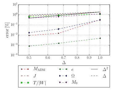
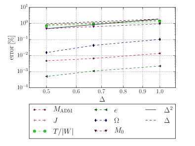
Figure 2: Normalized differences $|(f_{{\rm H}3.0}-f_{{\rm H}2.0})/f_{{\rm H}4.0}|$, $|(f_{{\rm H}3.5}-f_{{\rm H}2.5})/f_{{\rm H}4.0}|$, and $|(f_{{\rm H}4.0}-f_{{\rm H}3.0})/f_{{\rm H}4.0}|$ are plotted for $\Omega$, $M_{\rm ADM}$, $J$, $T/|W|$, $M_{0}$ and $e:=\sqrt{1-({\bar{R}}_{z}/{\bar{R}}_{x})^{2}}$ against the resolutions $\Delta_{{\rm H}3.0}$, $\Delta_{{\rm H}2.5}$, and $\Delta_{{\rm H}2.0}$. Black solid line is proportional to $\Delta^{2}$, while black dashed line is proportional to $\Delta$. The left panel refers to the LX EOS (Table 1) with central rest-mass density $\epsilon_{c}=1.301\times 10^{-3}$ and axis ratio in the coordinate length $R_{z}/R_{x}=0.75$. The right panel is the same but for the MIT bag-model EOS with $\epsilon_{c}=7.361\times 10^{-4}$ and the same deformation as the LX plot.

For the convergence analysis in this work we use the five resolutions shown in Table 4. The outer boundary of the domain is placed at $r_{b}=10^{6}$, while the surface of the star is always inside the sphere $r=1$. The radius along the $x$-axis is exactly $r=1$ in the normalized variables. There are exactly ${N_{r}^{\rm f}}$ intervals along the radii in the $x$, $y$, and $z$ directions. The number of Legendre terms used in the expansions is kept constant ($L=12$) in all resolutions since convergence with respect of those has been already investigated in Tsokaros and Uryū (2007). When going from the low-resolution setup H2.0 to the high-resolution one H4.0, the spacings $\Delta r,\Delta\theta,\Delta\phi$ decrease as $2/3,\ 3/4,\ 2/3,\ 3/4$.

As a result, if we denote as $f_{\mu}$, $f_{\nu}$ a quantity evaluated at two different resolutions, then

$$f_{\mu}\,-\,f_{\nu}\,\approx\,A\left[\left(\frac{\Delta_{\mu}}{\Delta_{\nu}}\right)^{n}-1\right]\Delta^{n}_{\nu}\,,$$ (29)

where $A$ is a constant and $\Delta_{\mu}$ is the grid separation at resolution ${\rm H}\mu$. Choosing the combinations $f_{{\rm H}3.0}-f_{{\rm H}2.0}$, $f_{{\rm H}3.5}-f_{{\rm H}2.5}$, and $f_{{\rm H}4.0}-f_{{\rm H}3.0}$ so that we have $\Delta_{\mu}/\Delta_{\nu}=1/2$ and normalizing by $f_{{\rm H}4.0}$ we plot in Fig. 2 the relative error with respect to the grid spacing for $\Omega$, $M_{\rm ADM}$, $J$, $T/|W|$, $M_{0}$ and the eccentricity $e:=\sqrt{1-({\bar{R}}_{z}/{\bar{R}}_{x})^{2}}$, both for the LX EOS (left panel) and for the MIT bag-model EOS (right plot). The deformation is kept at $R_{z}/R_{x}=0.75$ for both EOSs, while the central densities are $\epsilon_{c}=1.301\times 10^{-3}$, and $\epsilon_{c}=7.361\times 10^{-4}$ for LX and MIT bag-model EOS respectively. The dashed black line reports a reference first-order convergence, while the solid black line refers to second-order convergence.

Note that quantities like the ADM mass, the angular velocity and the eccentricity converge to second order, while quantities like the angular momentum, the ratio $T/|W|$, and the rest-mass converge to an order that is closer to first. Furthermore, Fig. 2 shows that some quantities (e.g., the ADM mass of the LX EOS) shows a convergence order that is larger than second, but this is an artefact of the specific deformation. In general, we found second-order convergence in $M_{\rm ADM},\ \Omega,\ e$ and at least first order for $J,\ T/|W|,\ M_{0}$.

Note also that the two panels in Fig. 2 are very similar, even though the EOSs are quite different, with the MIT bag-model EOS being relatively soft (i.e., $p\propto\rho^{4/3}$), while the LX EOS is comparatively stiff (i.e., $p\propto\rho^{5}$). Hence, the overall larger error that is reported in Fig. 2 when compared to the corresponding Fig. 1 in Ref. Huang et al. (2008), is mostly due to the finite rest-mass density at the stellar surface. In the original rotating-NS code, in fact, the surface was determined through a first-order interpolation scheme. This approach, however, is not sufficiently accurate for rotating QSs and would not lead to the desired convergence order unless the surface finder scheme was upgraded to second order.

IV Triaxial solutions

The onset of a secular instability to triaxial solutions for the MIT bag-model EOS stars has been studied previously via a similar method in Ref. Gondek-Rosińska et al. (2003). Surface-fitted coordinates have been used to accurately describe the discontinuous density at the surface of the star, and a set of equations similar to the one of the conformal flat approximation used here was solved. In order to find the secular bar-mode instability point, the authors of Ref. Gondek-Rosińska et al. (2003) performed a perturbation on the lapse function of an axisymmetric solution and build a series of triaxial quasi-equilibrium configurations to see whether this perturbation is damped or grows.

Here, we build quasi-equilibrium sequences with constant rest mass (axisymmetric and triaxial) for both the MIT bag-model EOS and the LX EOS. We begin with the axisymmetric sequence in which we calculate a series of solutions with varying parameters, i.e., the parameters that determine the compactness (e.g., the central rest-mass density $\rho_{c}$) and the rotation ($R_{z}/R_{x}$). In doing so, we impose axisymmetry as a separate condition and manage to reach eccentricities as high as $e\simeq 0.96$ for $R_{z}/R_{x}=0.2656$ and compactness $\mathcal{C}=0.1$. In order to access the triaxial branch of solutions, we recompute the above sequence of solutions but this time without imposing axisymmetry. As the rotation rate increases ($R_{z}/R_{x}$ decreases) the triaxial deformation ($R_{y}/R_{x}<1$) is spontaneously triggered, since at large rotation rate the triaxial configuration possesses lower total energy and is therefore favoured over the axisymmetric solution. This approach is different from the approach followed in Ref. Gondek-Rosińska and Gourgoulhon (2002), where the triaxial $m=2$ perturbation was triggered after a suitable modification of a metric potential.

We keep decreasing $R_{z}/R_{x}$ to reach the mass shedding limit with the triaxial configuration. We can then move along the triaxial solution sequence by increasing $R_{y}/R_{x}$ which now acts as the new rotating parameter. The sequence is then terminated close to the axisymmetric sequence. The bifurcation point can be found by extrapolating this triaxial sequence towards the axisymmetric solutions. The largest triaxial deformation calculated in this work, for both the MIT bag-model EOS and the LX EOS, is $R_{y}/R_{x}=0.5078$ for the $\mathcal{C}=0.1$ case (a three-dimensional of the surface for this solution is shown in Fig. 3), $R_{y}/R_{x}=0.5234$ for $\mathcal{C}=0.15$, and $R_{y}/R_{x}=0.6757$ for $\mathcal{C}=0.2$. Similar with NSs Huang et al. (2007), the endpoint of the triaxial sequence happens in lower eccentricities as the compactness increases.

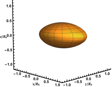
Figure 3: Illustration of the three-dimensional surface of a QS solution with the largest triaxial deformation for the MIT bag-model with corresponding spherical compactness $\mathcal{C}=0.2$. The axis ratio $R_{y}/R_{x}$ is 0.6757 and $R_{z}/R_{x}=0.4375$. The solid black lines on the surface corresponds to fixed values of the latitude angle and the fact that they are not parallel is a result of the triaxial deformation.

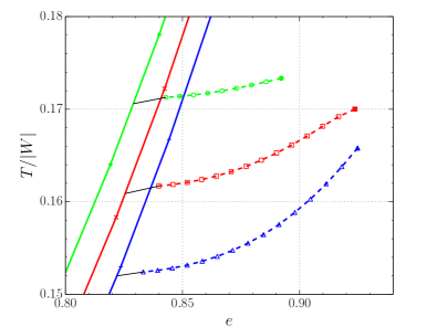
Figure 4: Left panel: $T/|W|$ versus eccentricity $e:=\sqrt{1-({\bar{R}}_{z}/{\bar{R}}_{x})^{2}}$ (in proper length) for MIT bag-model EOS sequences. Solid curves are axisymmetric solution sequences, and dashed curves are triaxial solution sequences, that correspond, to $\mathcal{C}=M/R=0.2$ (green curves), $0.15$ (red curves) and $0.1$ (blue curves) respectively. Note that $M$ is the spherical ADM mass. Right panel: magnification of the region near the onset of the triaxial solutions marked with empty symbols, while filled symbols mark the models at the mass-shedding limit. Solutions labelled with ”ML” are axisymmetric solutions (Maclaurin spheroids), while those labeled “JB” are triaxial solutions (Jacobi ellipsoids).

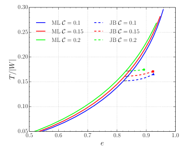
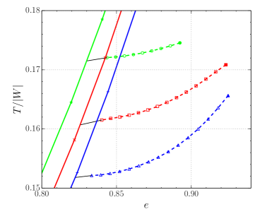
Figure 5: The same as Fig. 4 but for the LX EOS sequences.

In Figs. 4 and 5, the relation between the $T/|W|$ ratio versus the eccentricity of the star has been plotted for three different compactnesses ($\mathcal{C}=0.1,\ 0.15\ \mathrm{and}\ 0.2$) for both the MIT bag-model EOS and the LX EOS. Unlike in a Newtonian incompressible star, for which the bifurcation to triaxial deformation happens at $(T/|W|)_{\rm crit,Newt}\simeq 0.1375$ for any compactness, in general relativity the bifurcation point depends on the compactness. According to Gondek-Rosińska and Gourgoulhon (2002),

$$\left(\frac{T}{|W|}\right)_{\mathrm{\rm crit}}=\left(\frac{T}{|W|}\right)_{\rm crit,Newt}+0.126\,\mathcal{C}\left(1+\mathcal{C}\right)\,.$$ (30)

This relation holds true not only for NSs but also for QSs with the MIT bag-model EOS (see Fig. 1 of Gondek-Rosińska et al. (2003)). The largest $T/|W|$ for the onset of secular instability is found to be $\simeq 0.17$ for rotating QSs in the configurations that we considered for both the MIT bag-model EOS and the LX EOS, and it will be even larger for higher compactnesses. Both the LX EOS and the MIT bag-model EOS in our calculations follow this relationship within a maximum error of $3\%$. This implies that the secular instability to a ”Jacobi type” ellipsoidal figure in general relativity is not particularly affected by the stiffness of the EOS for quark matter.

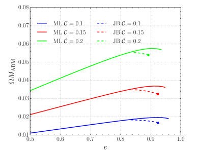
Figure 6: Plots of $\Omega M_{\rm ADM}$ versus eccentricity for MIT bag model sequences. Solid curves are axisymmetric solution sequences, and dashed curves are triaxial solution sequences, that correspond to $\mathcal{C}=M/R=0.2$ (top green curve), $0.15$ (middle red curve) and $0.1$ (bottom blue curve) respectively. Note that $M$ is the spherical ADM mass.

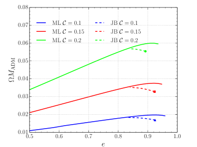
Figure 7: The same as Fig. 6 but for the LX EOS sequences.

EOS	$\mathcal{C}$	$R_{x}$	$R_{z}/R_{x}$	$\epsilon_{c}$	$\Omega$	$M_{\rm ADM}$	$J$	$T/|W|$	$I$	$Z_{\rm p}$
MIT	0.1	7.021 (8.077)	0.5647 (0.5693)	$6.200\times 10^{-4}$	0.02808	0.6515	0.4580	0.1520	16.31	0.1343
MIT	0.15	7.962 (9.922)	0.5565 (0.5640)	$6.811\times 10^{-4}$	0.02985	1.169	1.293	0.1609	43.30	0.2231
MIT	0.2	8.415 (11.43)	0.5478 (0.5590)	$7.696\times 10^{-4}$	0.03199	1.731	2.649	0.1706	82.83	0.3308
LX	0.1	5.698 (6.557)	0.5644 (0.5689)	$9.144\times 10^{-4}$	0.03451	0.5312	0.3039	0.1518	8.805	0.1343
LX	0.15	6.515 (8.130)	0.5566 (0.5639)	$9.542\times 10^{-4}$	0.03630	0.9686	0.8850	0.1607	24.38	0.2251
LX	0.2	6.972 (9.528)	0.5469 (0.5574)	$9.977\times 10^{-4}$	0.03838	1.481	1.932	0.1715	50.34	0.3401
$n=0.3$	0.1	6.624 (7.634)	0.5634(0.5693)	$9.221\times 10^{-4}$	0.03180	0.5841	0.3708	0.1507	11.66	0.1328
$n=0.3$	0.2	7.312 (9.979)	0.5394(0.5535)	$1.243\times 10^{-3}$	0.03926	1.435	1.835	0.1688	46.72	0.3311
$n=0.5$	0.1	10.30 (11.83)	0.5461(0.5536)	$5.153\times 10^{-4}$	0.02197	0.8416	0.7644	0.1493	34.80	0.1281

Table 5: Quantities at the point of bifurcation of triaxial sequences from axisymmetric ones for the two EOSs considered. The compactness of the spherical star with the same rest mass $\mathcal{C}$ are the model parameters. In the above, $R_{x}$ is the equatorial radius, and $R_{z}/R_{x}$ is the ratio of polar to the equatorial radius. Each has two values; one is measured in the coordinate length, and the other in parenthesis is in proper length. $\epsilon_{c}$ is the energy density at the center of the compact star, $\Omega$ is the angular velocity. In the last three lines we report the bifurcation point of simple polytropes with polytropic index $n$ as computed in Huang et al. (2008) for comparison. Note that we have chosen appropriate values for $\kappa$ such that the TOV maximum mass for those polytropic EOS reach 2.5 $M_{\odot}$. The definitions of $M_{\rm ADM}$, $J$, $T/|W|$, and $I$ can be found in the Appendix A of Tsokaros et al. (2015). $Z_{\rm p}$ is the polar redshift.

It is worth noting that when compared with the rotating NSs calculated in Ref. Uryū et al. (2016), rotating QSs have longer triaxial sequences. In another word, the triaxial sequence of rotating QSs terminates at larger eccentricity as well as larger triaxial deformation (in another word, smaller $R_{y}/R_{x}$ ratio). A rotating NS with $\Gamma=4$ and compactness $\mathcal{C}=0.1$ bifurcates from axisymmetry at $e\simeq 0.825$ and can rotate as fast as to reach eccentricities $e<0.9$ (see Fig. 6 in Uryū et al. (2016)). For the QS models considered here and both EOSs, we have a bifurcation point at $e\simeq 0.825$ and the mass shedding limit at $e\simeq 0.93$. For more compact NSs with $\mathcal{C}=0.2$, the bifurcation point happens at $e\simeq 0.835$ and the mass shedding limit at $e\simeq 0.88$. The corresponding compactness QS models bifurcate at $e\simeq 0.83$ and rotate as fast as $e\simeq 0.89$.

A few remarks are useful to make at this point. First, we note that these values of eccentricity are strictly valid under the assumption of the conformal flatness approximation, which is however accurate for smaller compactnesses. These estimates are less accurate when the compactness increases and are slightly different when adopting more accurate formulations, such as the waveless approximation (see Fig. 6 in Uryū et al. (2016)). Second, another difference between triaxial NSs and QSs is that for triaxial NSs, the ratio $T/|W|$ is essentially constant along the triaxial sequence, especially for higher compactnesses (for lower compactnesses there is an increase towards the mass shedding limit, but this is very slight). For rotating triaxial QSs, on the other hand, although this qualitative behaviour is still true, a greater curvature towards higher $T/|W|$ ratios can be seen. For example, for the $\mathcal{C}=0.1$ models mentioned above, the difference between the critical value of $T/|W|$ and the one at mass-shedding limit is $(T/|W|)_{\rm ms}-(T/|W|)_{\rm crit}\simeq 0.0015$ for NSs while it is $0.0137$ for QSs. Third, in Ref. Gondek-Rosińska et al. (2003) it has been shown that at the bifurcation point the relation between the scaled angular frequency, $f/\bar{\epsilon}_{s}^{1/2}$ where $\bar{\epsilon}_{s}=\epsilon_{s}/(c^{2}\,10^{14}\,\mathrm{g\,cm^{-3}}$), and the scaled gravitational mass $M_{\mathrm{ADM}}\bar{\epsilon}_{s}^{1/2}$, depends only very weakly on the bag constant. If we consider models with compactness $\mathcal{C}=0.1$ model (see top line in Table 5), $M_{\mathrm{ADM}}\bar{\epsilon}_{s}^{1/2}=1.193\,M_{\odot}$ and $f/\bar{\epsilon}_{s}^{1/2}=495.9\,\mathrm{Hz}$, while the scaled bifurcation frequency for such a scaled mass model is roughly $492-494\,\mathrm{Hz}$ as deduced from Fig. 7 in Gondek-Rosińska et al. (2003). Similarly, for the $\mathcal{C}=0.15$ models, the renormalized ADM mass and frequency are $2.140\,M_{\odot}$ and $527.2\,\mathrm{Hz}$, while the corresponding range is $523-527\,\mathrm{Hz}$ in Ref. Gondek-Rosińska et al. (2003); finally, for the $\mathcal{C}=0.2$ case, the values are $3.168\,M_{\odot}$ and $565.0\,\mathrm{Hz}$, respectively, while the range $558-566\,\mathrm{Hz}$ is found in Gondek-Rosińska et al. (2003). Overall, the comparison of these three values shows a very good agreement with the results presented in Fig. 7 of Ref. Gondek-Rosińska et al. (2003).

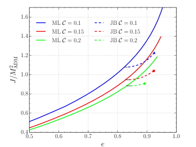
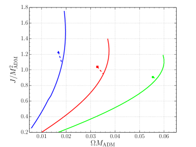
Figure 8: Spin angular momentum versus the eccentricity and angular velocity for the LX EOS sequences. Dashed curves and solid curves from the top to the bottom in each panel correspond to $\mathcal{C}=0.2$ (green), $0.15$ (red) and $0.1$ (blue) respectively.

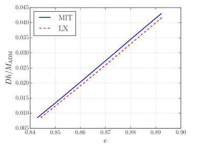
Figure 9: Estimate of the GW strain amplitude for the $\mathcal{C}=0.2$ triaxial sequence for both the MIT bag-model EOS (blue solid curve) and the LX EOS (red dashed curve). The quantities are estimated according to the quadrupole formula. Shown is the GW strain for the $\ell=m=2$ mode normalized by the distance $D$ and the ADM mass $M_{\mathrm{ADM}}$ of the source.

In order to understand the rotation properties of the triaxial solutions, we also report quantities such as dimensionless spin and dimensionless angular momentum in Fig. 6- 8. The dimensionless spin as a function of the eccentricity for MIT bag-model and LX model are shown in Fig. 6 and 7, respectively. The top panel of Fig. 8 reports the spin angular momentum as a function of the eccentricity for the LX EOS. Similar as $T/|W|$, the angular momentum increases with the eccentricity. The main difference is that the relative positioning of the curves as a function of compactness is reversed when compared with the $T/|W|$ plots. In other words for a given eccentricity the greatest angular momentum is achieved for the smallest compactness, while the greatest $T/|W|$ for the largest one. This is true both for axisymmetric and triaxial solutions. Also as we can see from the bottom panel of Fig. 8, more compact objects can reach greater rotational frequencies while less compact can reach larger angular momenta, which can exceed unity. According to Fig. 6 and 7 as well as the bottom panel of Fig. 8, triaxial sequences lose angular velocity and gain spin angular momentum as one moves towards the mass shedding limit.

An obviously interesting property of triaxially rotating compact stars is that they can act as strong sources of GWs. A full general-relativistic evolution needs to be employed in order to determine accurately the details of the GW emission from such triaxially rotating stars and this is beyond the scope of this paper (see however Ref. Tsokaros et al. (2017) for the case of NSs). At the same time, we can apply the quadrupole formula to make reasonable estimates using the quasi-equilibrium initial data we have computed. The relationship between the normalized GW strain and the eccentricity of the star is shown in the top panel of Fig. 9. Compared with the results of triaxially rotating NSs calculated in Tsokaros et al. (2017), we find that the GW strain for QSs are several times larger for similar values of the compactness. For example, model G4C025 in Tsokaros et al. (2017) with $e=0.8685$ radiates GW with normalized strain 0.007357, while the corresponding amplitude for both the MIT bag-model EOS and the LX EOS is around 0.025 with same eccentricity (see Fig. 9). Also shown in Fig. 9 for the two EOSs considered, are the relations between the strain and the eccentricity, which are very similar and both essentially linear.

V Triaxial supramassive solutions

Besides the constant rest-mass sequences mentioned above, we have also built sequences with constant central rest-mass density for both the MIT bag-model EOS and the LX EOS. We recall that when fixing the central rest-mass density, the mass of the solutions will increase as the axis ratio $R_{z}/R_{x}$ decreases. Furthermore, since we do not impose axisymmetry, the triaxial deformation will be spontaneously triggered when $T/|W|$ is large enough. Therefore, with such calculations we can determine whether triaxial supramassive QSs, i.e., triaxial solutions with ADM mass larger than the TOV maximum mass ($M_{\mathrm{TOV}}$) exist and the properties of such solutions (Note that all models shown in Figs. 4–8 are not supramassive).

According to Uryū et al. (2016), triaxial supramassive NS does exist for the case with polytropic EOS in the range $\Gamma\gtrsim 4$. Furthermore, for the case with a two segments piecewise polytropic EOS, sequences of triaxial supramassive NS solutions become longer, and hence the existence of supramassive triaxial NS becomes evident, when the EOS of the lower density region is stiff ($\Gamma=4$), and the higher density region is soft ($\Gamma=2.5$)Uryū et al. (2016). Therefore, it is likely that the triaxial supramassive QS also exists because the QS EOS used in this paper has an analogous property, namely, the effective $\Gamma$ is smaller (softer) in the higher density region, and larger (stiffer) in the lower density region (for the MIT model, see Gourgoulhon et al. (1999)). Besides having an interest of its own, determining the existence of such solutions could be relevant to establish whether a BNS merger could lead to the formation of such an object. Based on current mass measurement constraints Demorest et al. (2010); Antoniadis et al. (2013) and on known BNS systems, the mass of the post-merger product will very likely be larger than $M_{\mathrm{TOV}}$.

In order to study this, we have fixed the central rest-mass density close to the value corresponding to $M_{\mathrm{TOV}}$ and built rotating solution sequences for both the MIT bag-model EOS and the LX EOS, respectively. In this way, we were indeed able to find triaxial supramassive solutions for both EOSs, reporting in Table.6 the solutions with largest triaxial deformation, i.e., the smallest ratio $R_{y}/R_{x}$.

Finally, we note that although such models have large compactnesses and we are aware that the IWM formalism becomes increasingly inaccurate for large compactnesses (i.e., with $\mathcal{C}\gtrsim 0.3$), we also believe that the associated $\sim 3\%$ errors will not change the qualitative result, namely, that triaxial supramassive QS models exist for the EOSs considered here. At the same time, we plan to re-investigate this point in the future, when more accurate methods, such as waveless formulation, will be employed to compute QS solutions.

EOS	$R_{z}/R_{x}$	$R_{y}/R_{x}$	$R_{x}$	$\epsilon_{c}$	$\Omega$	$M_{\rm ADM}$	$J$	$T/|W|$	$I$	$M_{\mathrm{TOV}}$
MIT	0.4375 (0.4713)	0.7657 (0.7938)	9.978 (16.32)	$1.259\times 10^{-3}$	0.03870	2.862	6.847	0.1839	173.1	2.217
LX	0.4375 (0.4912)	0.7586 (0.8104)	7.660 (16.49)	$1.348\times 10^{-3}$	0.05001	3.727	11.30	0.1948	222.1	3.325

Table 6: Quantities of triaxial supramassive QS solutions with the largest triaxial deformation (smallest $R_{y}/R_{x}$ ratio) in our calculations. The above quantities are defined in the same way as in Table.5. The TOV maximum mass of each EOS is also shown as a comparison. Due to the limitation of IWM formulation, there might be $\sim 3\%$ errors on the quantities listed above (see related discussions in Sec.V).

VI Conclusion

We have presented a new version of the cocal code to compute axisymmetric and triaxial solutions of uniformly rotating QSs in general relativity with two EOSs, i.e., the MIT bag-model and the LX EOS. Comparisons have been made with NSs as well. Overall, three main properties are found when comparing solution sequences of QSs with of NSs. Firstly, QSs generally have a longer triaxial sequences of solutions than NSs. In another words, QSs can reach a larger triaxial deformation (or smaller $R_{y}/R_{x}$ ratio) before terminating the sequence at the mass-shedding limit; this is mostly due to the larger $T/|W|$ ratio that can be attained by QSs. Secondly, when considering similar triaxial configurations, QSs are (slightly) more efficient GW sources; this is mostly due to the finite surface rest-mass density and hence larger mass quadrupole for QSs. Thirdly, triaxial supramassive solutions can be found for QSs as well; this is due again to the fact that larger values of the $T/|W|$ ratio can be sustained before reaching the mass-shedding limit.

Besides having an interest of its own within solutions of self-gravitating objects in general relativity, triaxially rotating compact stars are important sources for ground-based GW observatories. Our calculations have shown that for rotating QSs with different EOSs, the bifurcation point to triaxial sequence happens at a spin period of $\sim 1\,{\rm ms}$, so that the corresponding GW frequency is $\sim 2\,{\rm kHz}$ and hence within the band of GW observatories such as Advanced LIGO or Virgo. Indeed, exploiting the largest triaxial deformation solution obtained in our calculations, the GW strain amplitude can be as large as $10^{-23}$ at a distance of $\sim 30\,{\rm Mpc}$.

Although this is an interesting prospect, it is still unclear whether such triaxial configurations can be produced in practice, since the radiation-reaction timescales needed for the triggering of the secular triaxial instability are still very uncertain, as are the other mechanisms that could contrast the instability. For example, if the triaxial deformation is induced in an isolated star, e.g., a newly born fast rotating star, GW radiation may take away the excess angular momentum very rapidly so that the star would go back to the axisymmetric sequence again after the $T/|W|$ ratio drops below the critical value. Similarly, when considering stars in binary systems, there is the prospect that an accreting system, such as the one spinning up pulsars, could drive the accreting compact star to exceed the critical $T/|W|$ ratio, hence leading to a break of axisymmetry. In this process, which is also known as forced GW emission, the triaxial deformation can be maintained via the angular momentum supplied by the accreted matter. Notwithstanding the large uncertainties involved with the details of this picture, such as the presence or not of bifurcation point or the realistic degree of deformation attained by the unstable stars, the fact that these details depend sensitively on the EOS Uryū et al. (2016), suggests that a detection of this type of signal could serve as an important probe for distinguishing the EOS of compact stars.

Finally, we note that the triaxial configurations could also be invoked to explain the spin-up limit for rotating compact stars, which is far smaller than the mass-shedding limit. The results presented here and in Ref. Huang et al. (2008) suggest that when triaxial deformations are taken into account, the rotational period of a compact star actually decreases as it gains angular momentum, e.g., by accretion, along the triaxial sequence. As a result, the “spin-up” process provided by the accretion of matter onto the pulsar can actually spin down the pulsar if the bifurcation point is reached. In this case, no accreting pulsar could spin up faster than the period at the bifurcation point. Of course, depending on the microphysical properties of the QS (e.g., the magnitude of the shear viscosity or of the breaking strain in the crust) it is also possible that other mechanisms of emission of gravitational waves, (e.g., other dynamical instabilities such as the barmode instability Watts et al. (2005); Corvino et al. (2010) or the $r$-mode instability Andersson (1998); Friedman and Morsink (1998); Andersson et al. (1999), or nonzero ellipticities) could intervene at lower spinning frequencies and therefore before the onset of instability to a triaxial deformation is reached Bildsten (1998); Andersson et al. (2011). As a result, the search for fast spinning pulsars with more powerful radio telescopes, such as the Square Kilometre Array (SKA) and the Five-hundred-meter Aperture Spherical radio Telescope (FAST) Kramer and Stappers (2015); Nan et al. (2011) could provide important clues on the properties of pulsars and test the validity of the solid QS assumption Xu (2003).