Quasi-Euclidean tilings over $2$–dimensional Artin groups and their applications

Abstract.

We describe the structure of quasiflats in two-dimensional Artin groups. We rely on the notion of metric systolicity developed in our previous work. Using this weak form of non-positive curvature and analyzing in details the combinatorics of tilings of the plane we describe precisely the building blocks for quasiflats in all two-dimensional Artin groups – atomic sectors. This allows us to provide useful quasi-isometry invariants for such groups – completions of atomic sectors, stable lines, and the intersection pattern of certain abelian subgroups. These are described combinatorially, in terms of the structure of the graph defining an Artin group. As an important tool, we introduce an analogue of the curve complex in the context of two-dimensional Artin groups – the intersection graph. We show quasi-isometric invariance of the intersection graph under natural assumptions.

As immediate consequences we present a number of results concerning quasi-isometric rigidity for the subclass of CLTTF Artin groups. We give a necessary and sufficient condition for such groups to be strongly rigid (self quasi-isometries are close to automorphisms), we describe quasi-isometry groups, we indicate when quasi-isometries imply isomorphisms for such groups. In particular, there exist many strongly rigid large-type Artin groups. In contrast, none of the right-angled Artin groups are strongly rigid by a previous work of Bestvina, Kleiner and Sageev.

1. Introduction

Overview

Let $\Gamma$ be a finite simple graph with each edge labeled by an integer $\geq 2$. An Artin group with defining graph $\Gamma$, denoted $A_{\Gamma}$, is given by the following presentation. Generators of $A_{\Gamma}$ are in one to one correspondence with vertices of $\Gamma$, and there is a relation of the form

$\underbrace{aba\cdots}_{m}=\underbrace{bab\cdots}_{m}$

whenever two vertices $a$ and $b$ are connected by an edge labeled by $m$.

Despite the seemingly simple presentation, the most basic questions (torsion, center, word problem and cohomology) on Artin groups remain open, though partial results are obtained by various authors. We refer to the survey papers by Godelle and Paris [MR3203644], and McCammond [jonproblems]. Other fundamental and natural questions for Artin groups which are equally exciting and difficult can be found in Charney [charney2016problems].

One common feature of various classes of Artin groups studied so far is that they all exhibit features of non-positive curvature of certain form:

• small cancellation [AppelSchupp1983, Appel1984, Pride, Peifer];

• bi-automaticity, automaticity, or some form of combing [Charney1992, MR1314589, charney2003k, MR2208796, holt2011artin, MR2985512, MR3351966];

• other notions of combinatorial non-positive curvature [Bestvina1999, Artinsystolic];

• $CAT(0)$ [charney1995k, BradyMcCammond2000, brady2002two, bell2005three, brady2010braids, haettel20166];

• hierarchical hyperbolicity (hence coarse median) [CharneyCrispAutomorphism, MR3650081, gordon2004artin, behrstock2015hierarchically];

• relative hyperbolicity [kapovich2004relative, charney2007relative];

• acylindrical hyperbolicity [calvez2016acylindrical, charney2019artin] and hyperbolicity in a statistical sense [cumplido2017loxodromic, yang2016statistically].

Conjecturally, all Artin groups should be non-positively curved in an appropriate sense, and this is intertwined with understanding many fundamental questions about Artin groups.

As most of the Artin groups have many abelian subgroups intersecting in a highly non-trivial way [davis2017determining], it is natural to compare them with other “higher rank spaces with non-positive-curvature features”  like symmetric spaces of non-compact type of rank $>1$, Euclidean buildings, mapping class groups and Teichmuller spaces of surfaces etc., and ask how much of the properties on geometry and rigidity of these spaces still hold for Artin groups and what are the new phenomena for Artin groups.

Motivated by such considerations, we study Gromov’s program of understanding quasi-isometric classification and rigidity of groups and metric spaces in the realm of $2$–dimensional Artin groups. We build upon a previous result [Artinmetric], where it was shown that all $2$–dimensional Artin groups satisfy a form of non-positive curvature called metric systolicity. In the current paper, we will show that certain “$0$–curvature chunks” of the group have a very specific structure, which gives rise to rigidity results.

Background

Previous works on quasi-isometric rigidity and classification of Artin groups fall into the following three classes, listed from the most rigid to the least rigid situation.

1. Some affine type Artin groups are commensurable to mapping class groups of surfaces [CharneyCrispAutomorphism]. Hence the quasi-isometric rigidity results for mapping class groups [behrstock2012geometry, hamenstaedt2005geometry] apply to them.

2. Atomic right-angled Artin groups [bestvina2008asymptotic] and their right-angled generalizations beyond dimension 2 [MR3692971, huang2016groups, huang2016commensurability, huang2016quasi].

3. Artin groups whose defining graphs are trees [behrstock2008quasi] (they are fundamental groups of graph manifolds) and a right-angled generalization beyond dimension 2 [MR2727658].

Most of the mapping class groups of surfaces enjoy the strong quasi-isometric rigidity property that any quasi-isometry of the group to itself is uniformly close to an automorphism. However, it follows implicitly from [bestvina2008asymptotic, Section 11] that none of the right-angled Artin groups satisfies such form of rigidity (see [MR3692971, Example 4.14] for a more detailed explanation).

One is more likely to obtain stronger rigidity result when the complexity of the intersection pattern of flats in the space is higher. Thus we are motivated to study Artin groups which are not necessarily right-angled, whose structure is generally more intricate than the one of right-angled ones. One particular case is the class of large-type Artin group, where the label of each edge in the defining graph is $\geq 3$. A commensuration rigidity result was proved by Crisp [MR2174269] for certain class of large-type Artin groups.

An Artin group is $n$–dimensional if it has cohomological dimension $n$. One-dimensional Artin groups are free groups. The class of two-dimensional Artin groups is much more abundant – all large-type Artin groups have dimension $\leq 2$. By Charney and Davis [CharneyDavis], $A_{\Gamma}$ has dimension $\leq 2$ if and only if for any triangle $\Delta\subset\Gamma$ with its sides labeled by $p,q,r$, we have $\frac{1}{p}+\frac{1}{q}+\frac{1}{r}\leq 1$. A model example to keep in mind is $A_{\Gamma}$ with $\Gamma$ being a complete graph with all its edges labeled by $3$.

Structure of quasiflats

Let $A_{\Gamma}$ be a two-dimensional Artin group. We study $2$–dimensional quasiflats in $A_{\Gamma}$, since the structure of top-dimensional quasiflats often plays a fundamental role in quasi-isometric rigidity of non-positively curved spaces, see the list of references after Theorem 1.1.

Let $X^{\ast}_{\Gamma}$ be the universal cover of the standard presentation complex of $A_{\Gamma}$. Modulo some technical details, quasiflats can be viewed as subcomplexes of $X^{\ast}_{\Gamma}$ which are homeomorphic to $\mathbb{R}^{2}$ and are quasi-isometric to $\mathbb{E}^{2}$ with the induced metric. Such subcomplexes are called quasi-Euclidean tilings over $X^{\ast}_{\Gamma}$ and studying such tilings of $\mathbb{R}^{2}$ is of independent interests. This viewpoint is motivated by both the geometric aspects of quasiflats explored in [bks] and diagrammatic aspects studied in [AppelSchupp1983, Pride, olshanskii2017flat].

To construct such a tiling, one can first search for tilings of Euclidean sectors appearing in $X^{\ast}_{\Gamma}$ (see Figure 1 for some examples), then glue these sectors along their boundaries in a cyclic fashion to form a quasi-Euclidean tiling. The following theorem says that this is essentially the only way one can obtain a quasiflat. Inside $X^{\ast}_{\Gamma}$ one can build a list of sectors which naturally arise from certain abelian subgroups, or centralizers of certain elements in $A_{\Gamma}$. We call them atomic sectors (cf. Section 5.2, in particular, Table 2 on page 2) since they are building blocks of quasiflats. Some of them are shown in Figure 1.

Theorem 1.1 (=Theorem 9.2).

Suppose $A_{\Gamma}$ is two-dimensional. Then any $2$–dimensional quasiflat $Q$ of $X^{\ast}_{\Gamma}$ is at finite Hausdorff distance away from a union of finitely many atomic sectors in $X^{\ast}_{\Gamma}$.

Figure 1. Some atomic sectors.

A simpler but less concise restatement of the above theorem is that every 2-dimensional quasiflat is made of “fragments” of subgroups of $A_{\Gamma}$ of form $F_{n}\times F_{m}$ ($n,m\geq 1$), where $F_{n}$ denotes the free group with $n$ generators.

Previously, structure theorems for quasiflats were proved for Euclidean buildings and symmetric spaces of non-compact type [kleiner1997rigidity, eskin1997quasi, wortman2006quasiflats], universal covers of certain Haken manifolds [kapovich1997quasi], certain CAT(0) complexes [bks, MR3654109] and hierarchically hyperbolic spaces [behrstock2017quasiflats].

Our viewpoint of tilings is convenient for, simultaneously, analyzing relevant group theoretic information and studying geometric aspects of quasiflats. The combinatorics of the group structure make up a substantial part. This is quite different from the more geometric situation in [bks, MR3654109, behrstock2017quasiflats]. Some of the atomic sectors are actually half-flats (see Definitions 5.13–5.16 below). This might seems strange compared to several previous quasiflat results, however, these sectors arise naturally when considering the group structure and they are convenient for our later applications.

Atomic sectors are not necessarily preserved under quasi-isometries. However, atomic sectors have natural completions (cf. Section 5.4) which are preserved under quasi-isometries (see Corollary 10.6 for a precise statement).

The following theorem says that certain $\mathbb{Z}$–subgroups corresponding to boundaries of atomic sectors are preserved under quasi-isometries. These $\mathbb{Z}$–subgroups act on what we call stable lines, and they are analogues of $\mathbb{Z}$–subgroups generated by Dehn twists in mapping class groups.

Theorem 1.2 (=Theorem 10.11).

Suppose $A_{\Gamma_{1}}$ and $A_{\Gamma_{2}}$ are two-dimensional Artin groups. Let $q\colon X^{\ast}_{\Gamma_{1}}\to X^{\ast}_{\Gamma_{2}}$ be an $(L,A)$–quasi-isometry. Then there exists a constant $D$ such that for any stable line $L_{1}\subset X^{\ast}_{\Gamma_{1}}$, there is a stable line $L_{2}\subset X^{\ast}_{\Gamma_{2}}$ with $d_{H}(q(L_{1}),L_{2})<D$.

For each $2$–dimensional Artin group $A_{\Gamma}$, we define an intersection graph $\mathcal{I}_{\Gamma}$ (Definition 10.13), which describes the intersection pattern of certain abelian subgroups. This object can be viewed as an analogue of the spherical building at infinity for symmetric spaces of non-compact type, or the curve graph in the case of mapping class groups. When $\Gamma$ is a triangle with its edges labeled by $3$, the group $A_{\Gamma}$ is commensurable to the mapping class group of the $5$–punctured sphere [CharneyCrispAutomorphism], and $\mathcal{I}_{\Gamma}$ is isomorphic to the curve complex of the $5$–punctured sphere.

Theorem 1.3.

Let $A_{\Gamma}$ and $A_{\Gamma^{\prime}}$ be two $2$–dimensional Artin groups and let $q\colon A_{\Gamma}\to A_{\Gamma^{\prime}}$ be a quasi-isometry. Then $q$ induces an isomorphism from the stable subgraph of $\mathcal{I}_{\Gamma}$ onto the stable subgraph of $\mathcal{I}_{\Gamma^{\prime}}$. In particular, if both $A_{\Gamma}$ and $A_{\Gamma^{\prime}}$ have finite outer automorphism group and $\Gamma$ has more than two vertices, then $q$ induces an isomorphism between their intersection graphs.

We refer to Theorem 10.16 for a more general version of Theorem 1.3.

Analogously, quasi-isometries of higher rank symmetric spaces of non-compact type and Euclidean buildings induce automorphisms of their spherical buildings at infinity [kleiner1997rigidity, eskin1997quasi]; and quasi-isometries of most mapping class groups induce automorphisms of their curve complexes [hamenstaedt2005geometry, behrstock2012geometry, behrstock2017quasiflats].

Recall that a finitely generated group $H$ is virtually $A_{\Gamma}$ if there exists a finite index subgroup $H^{\prime}\leq H$ and a homomorphism $\phi\colon H^{\prime}\to A_{\Gamma}$ with finite kernel and finite index image.

Corollary 1.4.

Let $A_{\Gamma}$ be a $2$–dimensional Artin group with finite outer automorphism group. Suppose $\Gamma$ has more than two vertices. If $q\colon A_{\Gamma}\to A_{\Gamma}$ is an $(L,A)$–quasi-isometry inducing the identity map on $\mathcal{I}_{\Gamma}$, then there exists $C=C(L,A,\Gamma)$ such that $d(q(x),x)\leq C$ for any $x\in A_{\Gamma}$. Thus the map $\operatorname{QI}(A_{\Gamma})\to\operatorname{Aut}(\mathcal{I}_{\Gamma})$ described in Theorem 1.3 is an injective homomorphism.

Thus if we know in addition that the homomorphism $A_{\Gamma}\to\operatorname{Aut}(\mathcal{I}_{\Gamma})$ induced by the action $A_{\Gamma}\curvearrowright\operatorname{Aut}(\mathcal{I}_{\Gamma})$ has finite index image, then any finitely generated groups quasi-isometric to $A_{\Gamma}$ is virtually $A_{\Gamma}$.

We refer to Corollary 10.17 for a more general version of Corollary 10.17.

Unlike the case of mapping class groups, $\operatorname{Aut}(\mathcal{I}_{\Gamma})$ could be much larger than $\operatorname{QI}(A_{\Gamma})$ in the context of Corollary 1.4. This happens for example in the right-angled case [MR3692971, Corollary 4.20]. However, we expect more rigidity to occur outside the right-angled world – see the next subsection for some special cases.

Rigidity of certain large-type Artin groups

We now discuss some immediate consequences of the results from the previous subsection. We will restrict ourselves to the class of CLTTF Artin groups introduced by Crisp [MR2174269] in order to use his results directly. Nevertheless, we believe that similar goals for more general classes of Artin groups can be achieved using the invariants described above. See the list of questions in Section 12 for possible further directions.

Definition 1.5.

An Artin group $A_{\Gamma}$ is CLTTF if all of the following conditions are satisfied:

• (C) $\Gamma$ is connected and has at least three vertices;

• (LT) $A_{\Gamma}$ is of large type;

• (TF) $\Gamma$ is triangle-free, i.e. $\Gamma$ does not contain any triangles.

In particular, CLTTF Artin groups are $2$–dimensional. As pointed out by Crisp, (C) serves to rule out $2$–generator Artin groups, which are best treated as a separate case. Here, we improve the commensurability rigidity of [MR2174269, Theorem 3] to quasi-isometric rigidity results and point out some new phenomena in the setting of quasi-isometries.

Theorem 1.6 (=Corollary 11.8).

Let $A_{\Gamma}$ and $A_{\Gamma^{\prime}}$ be CLTTF Artin groups. Suppose $\Gamma$ does not have separating vertices and edges. Then $A_{\Gamma}$ and $A_{\Gamma^{\prime}}$ are quasi-isometric if and only if $\Gamma$ and $\Gamma^{\prime}$ are isomorphic as labeled graphs.

By [MR2174269, Theorem 1], a CLTTF Artin group has finite outer automorphism group if and only if its defining graph has no separating vertices and edges. So Theorem 1.6 can be compared to [MR3692971, Theorem 1.1].

Theorem 1.7 (=Theorem 11.9).

Let $A_{\Gamma}$ be a CLTTF Artin group such that $\Gamma$ does not have separating vertices and edges. Let $\operatorname{QI}(A_{\Gamma})$ be the quasi-isometry group of $A_{\Gamma}$. Let $\operatorname{Isom}(A_{\Gamma})$ be the isometry group of $A_{\Gamma}$ with respect to the word distance for the standard generating set. Then the following hold.

1. Any quasi-isometry from $A_{\Gamma}$ to itself is uniformly close to an element in $\operatorname{Isom}(A_{\Gamma})$.

2. There are isomorphisms $\operatorname{QI}(A_{\Gamma})\cong\operatorname{Isom}(A_{\Gamma})\cong\operatorname{Aut}(D_{\Gamma})$, where $\operatorname{Aut}(D_{\Gamma})$ is the simplicial automorphism group of the Deligne complex $D_{\Gamma}$ of $A_{\Gamma}$.

There are counterexamples if we drop the condition that $\Gamma$ does not have separating vertices and edges, see [MR2174269, Lemma 42].

If $A_{\Gamma}$ is right-angled then $\operatorname{QI}(A_{\Gamma})$ is much smaller than $\operatorname{Aut}(D_{\Gamma})$, see [MR3692971, Corollary 4.20]. This suggests that the Artin groups in Theorem 1.7 are more rigid than right-angled Artin groups. On the other hand, the Artin groups in Theorem 1.7 may not be as rigid as mapping class groups, since elements in $\operatorname{Isom}(A_{\Gamma})$ are not necessarily uniformly close to automorphisms of $A_{\Gamma}$. A group $G$ is strongly rigid if any element in $\operatorname{QI}(G)$ is uniformly close to an element in $\operatorname{Aut}(G)$. Now we characterize all strongly rigid members of the class of large-type and triangle-free Artin groups.

Theorem 1.8 (=Theorem 11.10).

Let $A_{\Gamma}$ be a large-type and triangle-free Artin group. Then $A_{\Gamma}$ is strongly rigid if and only if $\Gamma$ satisfies all of the following conditions:

1. $\Gamma$ is connected and has $\geq 3$ vertices;

2. $\Gamma$ does not have separating vertices and edges;

3. any label preserving automorphism of $\Gamma$ which fixes the neighborhood of a vertex is the identity.

Moreover, if a large-type and triangle-free Artin group $A_{\Gamma}$ satisfies all the above conditions and $H$ is a finitely generated group quasi-isometric to $A_{\Gamma}$, then $H$ is virtually $A_{\Gamma}$.

Remark 1.9.

We note that the above quasi-isometric rigidity results do not use the full strength of Theorem 1.1 and Theorem 1.2, since proving the two theorems in the special cases of triangle-free Artin groups and Artin groups of hyperbolic type in the sense of [MR2174269] are much easier (though still non-trivial). Moreover, if an Artin group is triangle-free, then it acts geometrically on a $2$–dimensional CAT(0) complex [brady2000three], and it is C(4)-T(4) with respect to the standard presentation [Pride]. There are alternative starting points of studying quasiflats in such complexes, either by using [bks], or using [olshanskii2017flat]. However, several new ingredients are needed to deal with the general $2$–dimensional case. We present the above quasi-isometric rigidity results in order to demonstrate the potential of using Theorem 1.1 and Theorem 1.2 to obtain similar results for more general classes of Artin groups.

Comments on the proof

First we discuss the proof of Theorem 1.1. Let $X^{\ast}_{\Gamma}$ be the universal cover of the standard presentation complex of a $2$–dimensional Artin group $A_{\Gamma}$. To avoid technicalities, we assume the quasiflat is a subcomplex $Q$ of $X^{\ast}_{\Gamma}$ homeomorphic to $\mathbb{R}^{2}$ and quasi-isometric to $\mathbb{E}^{2}$, and we would like to understand the tiling of $Q$.

Step 0: The general idea is to use geometry of $A_{\Gamma}$ to control the tiling of $Q$. We start by showing that $A_{\Gamma}$ is non-positively curved in an appropriate sense. We would like to use CAT(0) geometry, however, at the time of writing, it is not known whether all $2$–dimensional Artin groups are CAT(0). Moreover, [brady2002two] implies that if certain $2$–dimensional Artin groups act geometrically on CAT(0) complexes, the dimension of the complexes is $\geq 3$. There are quite non-trivial technicalities in studying $2$–quasiflats in higher dimensional complexes and relating them to the combinatorics of groups, which we would like to bypass.

In [Artinmetric], we built a geometric model $X_{\Gamma}$ for $A_{\Gamma}$ with features of both CAT(0) geometry and two-dimensionality. More precisely, $X_{\Gamma}$ is a thickening of $X^{\ast}_{\Gamma}$. We equip the $2$–skeleton $X_{\Gamma}^{(2)}$ with a metric and it turns out that $X_{\Gamma}$ becomes non-positively curved in the sense that any $1$–cycle can be filled by a CAT(0) disc in $X_{\Gamma}^{(2)}$. Such a complex $X_{\Gamma}$ is an example of a metrically systolic complex.

Step 1. We study the local structure of $Q$ and show that outside a compact set, $Q$ is locally flat in an appropriate combinatorial sense.

Step 1.1. We approximate $Q$ by a CAT(0) subcomplex $Q^{\prime}$ in $X_{\Gamma}$ such that $Q^{\prime}$ is homeomorphic to $\mathbb{R}^{2}$. To do that, we pick larger and larger discs in $Q$, and we replace them by minimal discs in $X_{\Gamma}^{(2)}$, which are CAT(0), then we take a limit. By a version of Morse Lemma proved in [Artinmetric], $Q^{\prime}$ is at bounded Hausdorff distance from $Q$. An argument on area growth implies that $Q^{\prime}$ is flat outside a compact set. In fact, we obtain the following result in the more general setting of all metrically systolic complexes (see Theorem 2.7 for the detailed statement).

Theorem 1.10.

(cf. Theorem 2.7) Every quasiflat in a metrically systolic complex $X$ can be uniformly approximated by a simplicial map $q^{\prime}\colon Y\to X$ from a CAT(0) triangulation $Y$ of $\mathbb{R}^{2}$ being flat outside a compact set such that $q^{\prime}$ is injective on neighbourhoods of flat vertices.

Recently, independently, Elsner [elsner2017] has obtained an analogous result for systolic complexes. Theorem 1.10 applies to a larger class of spaces, however, Elsner’s result provides better control on the structure of quasiflats in the systolic setting.

Step 1.2. Though $Q^{\prime}$ is CAT(0) and flat outside a compact set, the cell structure on $Q^{\prime}$ is not ideal. A priori there may be triangles in $Q^{\prime}$ such that their angles are irrational multiples of $\pi$, and the cell structure is not compatible with the intersection pattern of quasiflats of $A_{\Gamma}$. So we go back to $X^{\ast}_{\Gamma}$, whose combinatorial structure is simpler than the one of $X_{\Gamma}$. By the design of $X_{\Gamma}$, there is a partial retraction $\rho$ from $X_{\Gamma}$ (defined on a subcomplex of $X_{\Gamma}$) to $X^{\ast}_{\Gamma}$. We argue that outside a compact subset, $\rho$ is well-defined on $Q^{\prime}$. Let $Q^{\prime\prime}=\rho(Q^{\prime})$. Then $Q^{\prime\prime}$ is a subcomplex with a “hole” (since $\rho$ may not be defined on all of $Q^{\prime}$). The map $\rho$ transfers information on local structure of $Q^{\prime}$ to information on local structure of $Q^{\prime\prime}$ (cf. Lemma 4.11). This step is discussed in Section 3 and Section 4.

Step 2. So far, we have a subcomplex $Q^{\prime\prime}$ about which we know that its local structure belongs to one of several types (as in Lemma 4.11). The next goal is to run a local-to-global argument in order to produce the sectors as required.

Step 2.1. We first produce a boundary ray for the sector, which is easier than producing the whole sector. To guess what kind of ray it could be, we look at a motivating example $X=\mathrm{SL}(3,\mathbb{R})/\mathrm{SO}(3,\mathbb{R})$. Quasiflats in $X$ are Hausdorff close to a finite union of Weyl cones [kleiner1997rigidity, eskin1997quasi]. The boundary of a Weyl cone is a singular ray, i.e. this ray is contained in the intersection of two flats. Analogously, we search for singular rays in $X_{\Gamma}$, which are possibly contained in the intersection of two free abelian subgroups of rank $2$. A list of plausible singular rays is given in Section 5.

Step 2.2. We show that there is at least one singular ray in $Q^{\prime\prime}$. The strategy is to start at one vertex of $Q^{\prime\prime}$, then walk away from this vertex and collect information about local landscape from Step 1.2 along the way to decide where to go further. Note that there is a “hole” in $Q^{\prime\prime}$ we want to avoid. This can be handled in the following way. Paths in $Q^{\prime\prime}$ have shadows in $Q^{\prime}$. Thus we can use the CAT(0) geometry in $Q^{\prime}$ to control where to go so we can avoid the “hole”. Section 6, Section 7 and Section 8 are devoted to the proof of the existence of singular rays in $Q^{\prime\prime}$. Another thing we need to be careful about is that the local structure discussed in Step 1.2 concerns not just the shapes of the cells around one vertex, but also the orientation of the edges around that vertex. In Section 7 we deal with the orientation issues.

Step 2.3. Now we know there is at least one singular ray in $Q^{\prime\prime}$. We start with this singular ray, and use the local characterization from Step 1.2 to “sweep out” a sector which ends in another singular ray. This uses a development argument. Now we iterate this process. It turns out that each sector in $Q^{\prime\prime}$ corresponds to a CAT(0) sector in $Q^{\prime}$ with angle bounded below by a uniform number. Since $Q^{\prime}$ has quadratic growth, after finitely many steps we produce enough sectors to fill $Q^{\prime\prime}$, which finishes the proof of Theorem 1.1. This step is discussed in Section 9.

Finally, we discuss how to deduce the quasi-isometric rigidity theorems for CLTTF Artin groups from Theorem 1.1. Again, we proceed in several steps. The first two steps can be generalized in an appropriate way to all $2$–dimensional Artin groups (cf. Theorem 10.11 and Theorem 10.16).

Step 1: Let $A_{\Gamma}$ be a CLTTF Artin. We consider the collection of maximal cyclic subgroups of $A_{\Gamma}$ with centralizers commensurable to $F_{2}\times\mathbb{Z}$. We show that these cyclic subgroups are preserved under quasi-isometries.

Step 2: Let $\Theta_{\Gamma}$ be a graph whose vertices correspond to cyclic subgroups from the previous step, and two vertices are adjacent if the associated cyclic subgroups generate a free abelian subgroup of rank $2$. This graph was introduced by Crisp [MR2174269]. We show that any quasi-isometry from $A_{\Gamma}$ to itself induces an automorphism of $\Theta_{\Gamma}$.

Step 3: Crisp [MR2174269] showed that any automorphism of $\Theta_{\Gamma}$ is induced by a canonical bijection from $A_{\Gamma}$ to itself, under appropriate additional conditions. In such way we approximate quasi-isometries by maps which preserve more combinatorial structure, and then deduce the quasi-isometric rigidity results listed above, see Section 11.

On the structure of the paper

In Section 2 we analyze the structure of quasiflats in metrically systolic complexes and we prove Theorem 1.10 above (Theorem 2.7 in the text). In Sections 3– 9 we describe the structure of complexes approximating quasiflats in two-dimensional Artin groups. In Section 9 we prove Theorem 1.1 (Theorem 9.2). In Section 10 we prove Theorem 1.2 (Theorem 10.11) and Theorem 1.3 (Theorem 10.16). In Section 11 we provide proofs of the results concerning CLTTF Artin groups: Theorem 1.6 (Corollary 11.8), Theorem 1.7 (Theorem 11.9), and Theorem 1.8 (Theorem 11.10).

Acknowledgment

J.H. would like to thank M. Hagen for a helpful discussion in July 2014, and R. Charney and T. Haettel for a helpful discussion in June 2016. J.H. also thanks the Max-Planck Institute for Mathematics, where part of the work was done, for its hospitality. Part of the work on the paper was carried out while D.O. was visiting McGill University. We would like to thank the Department of Mathematics and Statistics of McGill University for its hospitality during that stay. The authors were partially supported by (Polish) Narodowe Centrum Nauki, grants no. UMO-2015/18/M/ST1/00050 and UMO-2017/25/B/ST1/01335. This work was partially supported by the grant 346300 for IMPAN from the Simons Foundation and the matching 2015-2019 Polish MNiSW fund.

2. Quasiflats in metrically systolic complexes

We start with several notations. Let $X$ be a combinatorial cell complex. For a subset $Y\subset X$, the carrier of $Y$ in $X$ is the union of closed cells in $X$ which contain at least one point of $Y$ in their interior. For a vertex $x\in X$, the closed star of $v$ in $X$, denoted by $\operatorname{St}(x,X)$, is the union of closed cells in $X$ which contain $x$. When $X$ is a piecewise Euclidean polyhedral complex, i.e. $X$ is obtained by taking the disjoint union of a family of convex polyhedra in Euclidean spaces of various dimensions and gluing them along isometric faces, see [BridsonHaefliger1999, Definition I.7.37], the $\epsilon$–sphere around each vertex of $X$ inherits a natural polyhedral complex structure from $X$, for $\epsilon$ small (see [BridsonHaefliger1999, Definition I.7.15]). This polyhedral complex is called the link of $x$ in $X$, and is denoted by $\operatorname{lk}(x,X)$. If $X$ is a $2$–dimensional simplicial complex, then we always identify $\operatorname{lk}(x,X)$ with the full subgraph of the one-skeleton $X^{(1)}$ of $X$ spanned by vertices adjacent to $x$.

For a metric space $Z$ and a point $z\in Z$, we use $B(z,R)$ to denote the $R$–ball in $Z$ centered at $z$. For a subset $Y\subset Z$, we use $N_{R}(Y,R)$ to denote the $R$–neighborhood of $Y$ in $Z$.

2.1. Preliminaries on metrically systolic complexes

Let $X$ be a flag simplicial complex. We put a piecewise Euclidean structure on $X^{(2)}$ (the $2$–skeleton of $X$) in the following way. Since $X^{(2)}$ can be viewed as a disjoint collection of simplices with identifications between their faces, we assume every $2$–simplex (triangle) is isometric to a non-degenerate Euclidean triangle and all the identifications are isometries. This gives a length metric on $X^{(2)}$, which we denote by $d$. Since we will work with the $2$–skeleton of $X$, for a vertex $v\in X$, we define its link to be the full subgraph of $X^{(1)}$ spanned by all vertices adjacent to $v$ as explained as above. Every link is equipped with an angular metric, defined as follows. For an edge $\overline{v_{1}v_{2}}$, we define the angular length of this edge to be the angle $\angle_{v}(v_{1},v_{2})$ with the apex $v$. This turns the link into a metric graph, and the angular metric, which we denote by $d_{\angle}$, is the path metric of this metric graph (note that a priori we do not know $\angle_{v}(v_{1},v_{2})=d_{\angle}(v_{1},v_{2})$ for adjacent vertices $v_{1}$ and $v_{2}$). The angular length of a path $\omega$ in the link, which we denote by $\operatorname{length}_{\angle}(\omega)$, is the summation of angular lengths of edges in this path. In this paper we assume that the following weak form of triangle inequality holds for angular lengths of edges in $X$: for each $v\in X$ and every three pairwise adjacent vertices $v_{1},v_{2},v_{3}$ in the link of $v$ we have that $\angle_{v}(v_{1},v_{3})\leq\angle_{v}(v_{1},v_{2})+\angle_{v}(v_{2},v_{3})$. Then we call $X$ (with metric $d$) a metric simplicial complex.

Remark 2.1.

We allow that the above inequality becomes equality – intuitively, it corresponds to degenerate $2$–simplices in a link, which correspond to degenerate $3$–simplices in $X$.

For $k=4,5,6,\ldots$, a simple $k$–cycle $C$ in a simplicial complex is $2$–full if there is no edge connecting any two vertices in $C$ having a common neighbor in $C$ (that is, there are no local diagonals).

Definition 2.2 (Metrically systolic complex).

A link in a metric simplicial complex is $2\pi$–large if every $2$–full simple cycle in the link has angular length at least $2\pi$. A metric simplicial complex $X$ is locally $2\pi$–large if every its link is $2\pi$–large. A simply connected locally $2\pi$–large metric complex is called a metrically systolic complex.

In Theorem 2.3 below we state a fundamental property of metrically systolic complexes. It concerns filling diagrams for cycles, and it is a main tool used in proofs of various results about such complexes in subsequent sections and, previously, in [Artinmetric].

Let $X$ be a simplicial complex. A cycle in $X$ is a simplicial map from a triangulated circle to $X$ which is injective on each edge. A singular disc $D$ is a simplicial complex isomorphic to a finite connected and simply connected subcomplex of a triangulation of the plane. There is the (obvious) boundary cycle for $D$, that is, a map from a triangulation of $1$–sphere (circle) to the boundary of $D$, which is injective on edges. More precisely, we can view $D$ as a subset of the $2$–sphere $\mathbb{S}^{2}$. Then $\mathbb{S}^{2}\setminus D$ is an open cell, and the boundary of this open cell gives rise to the boundary cycle of $D$. For a cycle $C\colon K\to X$ in a simplicial complex $X$, a singular disc diagram for $C$ is a simplicial map $f\colon D\to X$ from a singular disc $D$ to $X$ such that $C\colon K\to X$ factors through the boundary cycle of $D$. By the relative simplicial approximation theorem [Zeeman1964], for every cycle in a simply connected simplicial complex there exists a singular disc diagram (cf. also van Kampen’s lemma e.g. in [LSbook, pp. 150-151]). It is an essential feature of metrically systolic complexes that singular disc diagrams may be modified to ones with some additional properties; see Theorem 2.3 below.

A singular disc diagram is called nondegenerate if it is injective on all simplices. It is reduced if distinct adjacent triangles (i.e., triangles sharing an edge) are mapped into distinct triangles. For a metric simplicial complex $X$ and a nondegenerate singular disc diagram $f\colon D\to X$ we equip $D$ with a metric in which $f|_{\sigma}$ is an isometry onto its image, for every simplex $\sigma$ in $D$. Then, $f$ is a CAT(0) singular disc diagram if $D$ is CAT(0), that is, if the angular length of every link in $D$ being a cycle (that is, the link of an interior vertex in $D$) is at least $2\pi$. An internal vertex in $D$ is flat when the angular length of its link is exactly $2\pi$.

Theorem 2.3 (CAT(0) disc diagram).

[Artinmetric, Theorem 2.8] Let $f\colon D\to X$ be a singular disc diagram for a cycle $C$ in a metrically systolic complex $X$. Then there exists a singular disc diagram $f^{\prime}\colon D^{\prime}\to X$ for $C$ such that

1. $f^{\prime}\colon D^{\prime}\to X$ is a CAT(0) nondegenerate reduced disc diagram;

2. $f^{\prime}$ does not use any new vertices in the sense that there is an injective map $i$ from the vertex set of $D^{\prime}$ to the vertex set of $D$ such that $f=f^{\prime}\circ i$ on the vertex set of $D$;

3. if $v\in D^{\prime}$ is a flat interior vertex, then $f^{\prime}$ is injective on the closed star of $v$ in $D^{\prime}$.

The number of $2$–simplices in $D^{\prime}$ is at most the number of $2$–simplices in $D$.

The following result is immediate.

Corollary 2.4.

Suppose $X$ is a metrically systolic complex with finitely many isometry types of cells. Then there exists a constant $L>0$ such that for each cycle $C$ with $\leq n$ edges, there is a singular disc diagram for $C$ with $\leq Cn^{2}$ triangles in the disc diagram and the image of the singular disc diagram is contained in the $(L\cdot n)$–neighborhood of $C$.

Note that whenever there is a statement regarding metric on $X$, we always mean the length metric $d$ with respect to the piecewise Euclidean structure on $X^{(2)}$. If there are finitely many isometry types of cells in $X^{(2)}$, then $(X^{(2)},d)$ is a complete geodesic metric space [BridsonHaefliger1999, Theorem I.7.19]. Moreover, $d$ is quasi-isometric to the path metric on $X^{(1)}$ such that each edge has length $1$ [BridsonHaefliger1999, Proposition I.7.31].

We also need the following version of the Morse Lemma for discs in metrically systolic complexes. See [Artinmetric, Theorem 3.9] for the proof.

Lemma 2.5.

[Morse Lemma for $2$–dimensional quasi-discs] Let $D$ be a combinatorial ball in the Euclidean plane tiled by equilateral triangles. Let $f\colon D\to X$ be a disc diagram for a cycle $C$ in $X$ being an $(L,A)$–quasi-isometric embedding. Let $g\colon D^{\prime}\to X$ be a singular disc diagram for $C$. Then $\mathrm{im}(f)\subseteq N_{a}(\mathrm{im}(g))$, where $a>0$ is a constant depending only on $L$ and $A$.

2.2. The structure of quasiflats

Recall that $B_{X}(x,r)$ denotes the ball of radius $r$ centered at $x$ in a metric space $X$. Here and elsewhere we use the notation $d_{H}$ for the Hausdorff distance. The following is a consequence of [bks, Theorem 4.1].

Theorem 2.6.

Suppose $X$ is a $2$–dimensional piecewise Euclidean CAT(0) complex such that $X$ is homeomorphic to $\mathbb{R}^{2}$ and $X$ has finitely many isometry types of cells. If there is a constant $L>0$ and a base point $x\in X$ such that $\operatorname{Area}(B_{X}(x,r))\leq Lr^{2}$, for any $r>0$, then $X$ is flat outside a compact subset.

Theorem 2.7.

Let $X$ be a locally finite metrically systolic complex with finitely many isometry types of cells. Let $q\colon\mathbb{E}^{2}\to X$ be an $(L,A)$–quasi-isometric embedding. Then there exist a constant $M_{0}$ depending only on $L,A$ and $X$, a simplicial complex $Y$, and a reduced nondegenerate simplical map $q^{\prime}\colon Y\to X$ such that

1. $Y$ is a $2$–dimensional simplicial complex homeomorphic to $\mathbb{R}^{2}$;

2. if we endow $Y$ with the piecewise Euclidean structure such that each simplex in $Y$ is isometric to its $q^{\prime}$–image, then $Y$ is CAT(0);

3. $Y$ is flat outside a compact subset;

4. for any flat vertex $v\in Y$, $q^{\prime}$ is injective on $\operatorname{St}(v,Y)$; and if we view $\operatorname{lk}(v,Y)$ as a simple close cycle in $X$, then it does not bound a disc diagram without interior vertices;

5. $d_{H}(\operatorname{Im}q,\operatorname{Im}q^{\prime})<M_{0}$.

Proof.

Let $q\colon\mathbb{E}^{2}\to X$ be an $(L,A)$–quasi-isometric embedding. We view $\mathbb{E}^{2}$ as a simplicial complex which is tiled by equilateral triangles. Using Corollary 2.4 and a skeleton by skeleton approximation argument, we can assume $q$ is also $L^{\prime}$–Lipschitz. Since $X$ has finitely many isometry types of cells, it follows from $q$ being $L^{\prime}$–Lipschitz and [BridsonHaefliger1999, Lemma I.7.54] that if the diameter of equilateral triangles in $\mathbb{E}^{2}$ is small enough, then the $q$–image of the closed star of a vertex in $\mathbb{E}^{2}$ is contained in the closed star of a vertex in $X$. By a standard simplicial approximation argument, we can assume in addition that $q$ is a simplicial map. The new quasi-isometric constants of $q$ depend only on the old constants and $X$.

Pick a base vertex $x\in\mathbb{E}^{2}$. Let $D_{n}\subset\mathbb{E}^{2}$ be the full subcomplex spanned by vertices with combinatorial distance $\leq n$ from $x$. Up to attaching a thin annulus to $D_{n}$ along $\partial D_{n}$, we assume $q_{n}=q|_{D_{n}}$ maps each edge in $\partial D_{n}$ to an edge in $X$. As in Theorem 2.3, for each $n$, we modify $q_{n}\colon D_{n}\to X$ to obtain a reduced nondegenerate CAT(0) singular disc diagram $q^{\prime}_{n}\colon D^{\prime}_{n}\to X$ such that $q^{\prime}_{n}$ and $q_{n}$ have the same boundary cycle. Moreover, we assume $q^{\prime}_{n}\colon D^{\prime}_{n}\to X$ has the least number of triangles among all singular disc diagrams satisfying the conditions of Theorem 2.3 and has the same boundary cycle as $q_{n}$. Then

• $d_{H}(\operatorname{Im}q^{\prime}_{n},\operatorname{Im}q_{n})<M$ with $M$ depending only on $L$ and $A$;

• Theorem 2.7 (4) holds for flat interior vertices in $D^{\prime}_{n}$.

The first property follows from Lemma 2.5. For the second property, if $\operatorname{lk}(v,D^{\prime}_{n})$ bounds a singular disc diagram without interior vertices for some flat interior vertex $v\in D^{\prime}_{n}$, then we can replace $\operatorname{St}(v,D^{\prime}_{n})$ with such diagram to obtain a singular disc diagram $\bar{q}_{n}\colon\bar{D}_{n}\to X$ with fewer triangles. Now, use Theorem 2.3 to modify $\bar{q}_{n}$ further to obtain a singular disc diagram $\hat{q}_{n}\colon\widehat{D}_{n}\to X$. Then $\widehat{D}_{n}$ contradicts the minimality of $D^{\prime}_{n}$.

Let $A_{0}=\max\{L,A,L^{\prime},M\}$. For $R\geq 100A_{0}$ and $n\geq 100A_{0}R$, let $K_{R,n}\subset D^{\prime}_{n}$ be the largest possible subcomplex such that $q^{\prime}_{n}(K_{R,n})$ is contained in the $R$–ball $B_{X}(q(x),R)$ of $X$ centered at $q(x)$. Then the following hold:

1. $K_{R,n}$ is locally CAT(0);

2. there is $M^{\prime}$ depending only on $L$ and $A$ such that $q(\mathbb{E}^{2})\cap B_{X}(q(x),\frac{R}{2})$ is contained in the $M^{\prime}$–neighborhood of $q^{\prime}_{n}(K_{R,n})$;

3. $\operatorname{lk}(v,K_{R,n})$ is a circle for any vertex $v\in K_{\frac{R}{2},n}$;

(b) follows from the inequality $d_{H}(\operatorname{Im}q^{\prime}_{n},\operatorname{Im}q_{n})<M$, and (c) follows from the fact that $q^{\prime}_{n}(v)$ is far away from $q^{\prime}_{n}(\partial D^{\prime}_{n})$. Since $q^{\prime}_{n}$ does not use new vertices in the sense of Theorem 2.3, the cardinality of $K^{(0)}_{R,n}$ is $\leq$ the number of vertices in $\mathbb{E}^{2}$ whose $q$–images are contained in $B_{X}(q(x),R)$. Moreover, $X$ is locally finite by our assumption. Thus by passing to a subsequence, we assume for any $n$ and $m$, there is a simplicial isomorphism $\phi_{n,m}\colon K_{R,n}\to K_{R,m}$ such that $q^{\prime}_{n}=q^{\prime}_{m}\circ\phi_{n,m}$ on $K_{R,n}$. Now we let $R\to\infty$ and use a diagonal argument to produce $q^{\prime}\colon Y\to X$ such that for any $R$ and any subcomplex $K\subset Y$ such that $q^{\prime}(K)$ is contained in the $R$–ball of $x$, there exists $n$ and a simplicial embedding $\phi_{K}\colon K\to D^{\prime}_{n}$ such that $q^{\prime}=q^{\prime}_{n}\circ\phi_{K}$ on $K$.

Now we show that $q^{\prime}$ satisfies all the requirements. First we show $Y$ is simply-connected. Take a closed curve $C\subset Y$ and take $R$ such that $q^{\prime}(C)\subset B_{X}(q(x),\frac{R}{100})$. Let $K\subset Y$ be the maximal subcomplex such that $q(K)\subset B_{X}(q(x),R)$ and let $D^{\prime}_{n}$ be as above. Since $D^{\prime}_{n}$ is CAT(0), we can find a geodesic homotopy in $D^{\prime}_{n}$ that contracts $C$ to a point in $C$. Note that $q^{\prime}_{n}$ is Lipschitz since it is simplicial. Thus the $q$–image of this homotopy is contained in $B_{X}(q(x),R)$, and the homotopy actually happens inside $K$. This together with property (a) above implies that $Y$ is CAT(0). By (c), $Y$ is homeomorphic to $\mathbb{R}^{2}$. By Theorem 2.3, $q^{\prime}(Y)$ is contained in the full subcomplex of $X$ spanned by $q(\mathbb{E}^{2})$. This and property (b) above imply $d_{H}(\operatorname{Im}q^{\prime},\operatorname{Im}q)<M_{0}$ for $M_{0}=M_{0}(L,A,X)$. Also Theorem 2.7 (4) follows from Theorem 2.3 (3) and the properties of $q^{\prime}_{n}$ discussed before.

It remains to show $Y$ is flat outside a compact set. By Theorem 2.6, it suffices to estimate the area of balls in $Y$. Pick a base point $y\in Y$ such that $d(q^{\prime}(y),q(x))<M_{0}$. Let $B_{R}$ be the $R$–ball in $Y$ centered at $y$ with respect to the CAT(0) metric and let $K_{R}$ be the union of faces of $Y$ that intersect $B_{R}$. Then there exists $n$ and a simplicial embedding $\phi_{R}\colon K_{R}\to D^{\prime}_{n}$ such that $q^{\prime}=q^{\prime}_{n}\circ\phi_{R}$ on $K_{R}$. Thus we also view $y,B_{R}$ and $K_{R}$ as subsets of $D^{\prime}_{n}$. Since $B_{R}\subset B_{D^{\prime}_{n}}(y,R)$, it suffices to show $\operatorname{Area}(B_{D^{\prime}_{n}}(y,R))\leq L_{3}R^{2}$ for $L_{3}$ independent of $R$ and $n$.

Note that there exists a constant $0<\delta<1$ independent of $n$ and $R$ such that $B_{D^{\prime}_{n}}(y,\delta n)$ does not touch the boundary of $D^{\prime}_{n}$. This uses the fact that $q_{n}$ and $q^{\prime}_{n}$ agree on the boundary, $q_{n}$ is a quasi-isometry and $q^{\prime}_{n}$ is simplicial (hence Lipschitz). We assume $n$ is large enough so that $R<\delta n$. For $r<\delta n$, let $h_{r}\colon B_{D^{\prime}_{n}}(y,\delta n)\to B_{D^{\prime}_{n}}(y,r)$ be the map which moves every point $p\in B_{D^{\prime}_{n}}(y,\delta n)$ towards $y$ along the geodesic $\overline{py}$ by a factor of $\frac{r}{\delta n}$. Then $h_{r}$ is $\frac{r}{\delta n}$–Lipschitz and we have

$$\frac{\operatorname{Area}(B_{D^{\prime}_{n}}(y,\delta n))}{(\delta n)^{2}}\geq\frac{\operatorname{Area}(B_{D^{\prime}_{n}}(y,r))}{r^{2}}$$

On the other hand,

$$\operatorname{Area}(B_{D^{\prime}_{n}}(y,\delta n))\leq\operatorname{Area}(D^{\prime}_{n})\leq L_{1}(\ell(\partial D^{\prime}_{n}))^{2}=L_{1}(\ell(\partial D_{n}))^{2}\leq L_{2}n^{2}.$$

Here $L_{1}$ is the isoperimetric constant for CAT(0) space and $\ell(\partial D^{\prime}_{n})$ denotes the length of $\partial D^{\prime}_{n}$. Thus there exists $L_{3}$ independent of $n$ and $R$ such that $\operatorname{Area}(B_{D^{\prime}_{n}}(y,r))\leq L_{3}r^{2}$ for any $r<\delta n$. This finishes the proof. ∎

3. The complexes for dihedral Artin groups

In this section we recall the local structure of the complexes for dihedral Artin groups constructed in [Artinmetric] and study disc diagrams over such complexes.

3.1. The complex for dihedral Artin groups

Let $DA_{n}$ be the $2$–generator Artin group presented by $\langle a,b\mid\underbrace{aba\cdots}_{n}=\underbrace{bab\cdots}_{n}\rangle$.

Let $P_{n}$ be the standard presentation complex for $DA_{n}$. Namely the $1$–skeleton of $P_{n}$ is the wedge of two oriented circles, one labeled $a$ and one labeled $b$. Then we attach the boundary of a closed $2$–cell $C$ to the $1$–skeleton with respect to the relator of $DA_{n}$. Let $C\to P_{n}$ be the attaching map. Let $X^{\ast}_{n}$ be the universal cover of $P_{n}$. Then any lift of the map $C\to P_{n}$ to $C\to X^{\ast}_{n}$ is an embedding (cf. [Artinsystolic, Corollary 3.3]). These embedded discs in $X^{\ast}_{n}$ are called precells. Figure 2 depicts a precell $\Pi^{\ast}$. $X^{\ast}_{n}$ is a union of copies of $\Pi^{\ast}$’s. We pull back the labeling and orientation of edges in $P_{n}$ to obtain labeling and orientation of edges in $X^{\ast}_{n}$.

Figure 2. Precell $\Pi^{\ast}$.

We label the vertices of $\Pi^{\ast}$ as in Figure 2. The vertices $\ell$ and $r$ are called the left tip and the right tip of $\Pi^{\ast}$. The boundary $\partial\Pi^{\ast}$ is made of two paths. The one starting at $\ell$, going along $\underbrace{aba\cdots}_{n}$ (resp. $\underbrace{bab\cdots}_{n}$), and ending at $r$ is called the upper half (resp. lower half) of $\partial\Pi^{\ast}$. The orientation of edges inside one half is consistent, thus each half has an orientation.

We summarize several facts on how precells intersect each other.

Lemma 3.1.

[Artinsystolic, Corollary 3.4] Let $\Pi^{\ast}_{1}$ and $\Pi^{\ast}_{2}$ be two different precells in $X^{\ast}_{n}$. Then

1. either $\Pi^{\ast}_{1}\cap\Pi^{\ast}_{2}=\emptyset$, or $\Pi^{\ast}_{1}\cap\Pi^{\ast}_{2}$ is connected;

2. if $\Pi^{\ast}_{1}\cap\Pi^{\ast}_{2}\neq\emptyset$, $\Pi^{\ast}_{1}\cap\Pi^{\ast}_{2}$ is properly contained in the upper half or in the lower half of $\Pi^{\ast}_{1}$ (and $\Pi^{\ast}_{2}$);

3. if $\Pi^{\ast}_{1}\cap\Pi^{\ast}_{2}$ contains at least one edge, then one end point of $\Pi^{\ast}_{1}\cap\Pi^{\ast}_{2}$ is a tip of $\Pi^{\ast}_{1}$, and another end point of $\Pi^{\ast}_{1}\cap\Pi^{\ast}_{2}$ is a tip of $\Pi^{\ast}_{2}$, moreover, among these two tips, one is a left tip and one is a right tip.

Lemma 3.2.

[Artinmetric, Corollary 4.3] Let $\Pi^{\ast}_{1}$ and $\Pi^{\ast}_{2}$ be two different precells in $X^{\ast}_{n}$. If $\Pi^{\ast}_{1}\cap\Pi^{\ast}_{2}$ contains at least one edge, and $\Pi^{\ast}_{3}\cap\Pi^{\ast}_{2}=\Pi^{\ast}_{1}\cap\Pi^{\ast}_{2}$, then $\Pi^{\ast}_{3}=\Pi^{\ast}_{1}$.

Lemma 3.3.

Let $\{\Pi^{\ast}_{i}\}_{i=1}^{3}$ be three different precells in $X^{\ast}_{n}$. Suppose

1. $\Pi^{\ast}_{1}\cap\Pi^{\ast}_{2}$ contains an edge;

2. $\Pi^{\ast}_{1}\cap\Pi^{\ast}_{3}$ contains an edge;

3. $(\Pi^{\ast}_{1}\cap\Pi^{\ast}_{2})\cap(\Pi^{\ast}_{1}\cap\Pi^{\ast}_{3})$ is either one point or empty.

Then $\Pi^{\ast}_{2}\cap\Pi^{\ast}_{3}$ is either one point or empty.

Proof.

By Lemma 3.1, there are two cases to consider. Either $\Pi^{\ast}_{1}\cap\Pi^{\ast}_{2}$ and $\Pi^{\ast}_{1}\cap\Pi^{\ast}_{3}$ are in the same half of $\Pi^{\ast}_{1}$, or they are in different halves. The latter case follows from [Artinsystolic, Corollary 3.5]. For the former case, we assume without loss of generality that $\Pi^{\ast}_{1}\cap\Pi^{\ast}_{2}$ and $\Pi^{\ast}_{1}\cap\Pi^{\ast}_{3}$ are contained in the upper half of $\Pi^{\ast}_{1}$. By Lemma 3.1 (3) and Lemma 3.3 (3), we assume $\Pi^{\ast}_{1}\cap\Pi^{\ast}_{2}$ (resp. $\Pi^{\ast}_{1}\cap\Pi^{\ast}_{3}$) contains the left tip (resp. right tip) of $\Pi^{\ast}_{1}$, see Figure 3. Assume by contradiction that $\Pi^{\ast}_{2}\cap\Pi^{\ast}_{3}$ contains an edge. By [Artinsystolic, Corollary 3.5], if $\Pi^{\ast}_{2}\cap\Pi^{\ast}_{3}$ and $\Pi^{\ast}_{2}\cap\Pi^{\ast}_{1}$ are in different halves of $\Pi^{\ast}_{2}$, then $\Pi^{\ast}_{1}\cap\Pi^{\ast}_{3}$ can not contain any edge, which yields a contradiction. Thus $\Pi^{\ast}_{2}\cap\Pi^{\ast}_{3}$ and $\Pi^{\ast}_{2}\cap\Pi^{\ast}_{1}$ are in the same half of $\Pi^{\ast}_{2}$. It follows that $P$ is not an embedded path, where $P$ travels from the left tip of $\Pi^{\ast}_{2}$ to the left tip of $\Pi^{\ast}_{1}$, then travel to the right tip of $\Pi^{\ast}_{1}$ along the upper half of $\Pi^{\ast}_{1}$, then travel to the right tip of $\Pi^{\ast}_{3}$. On the other hand, since $P$ represents a word in the positive Artin monoid, $P$ is an embedded path by the injectivity of positive Artin monoid [deligne, brieskorn1972artin], which leads to a contradiction.

Figure 3.

∎

We subdivide each precell $\Pi^{\ast}$ in $X^{\ast}_{n}$ into a simplicial complex by placing a vertex in the middle of the precell, and adding edges which connect this new vertex and vertices in the boundary $\partial\Pi^{\ast}$. This subdivision turns $X^{\ast}_{n}$ into a simplicial complex $X^{\scalebox{0.53}{$\triangle$}}_{n}$. A cell of $X^{\scalebox{0.53}{$\triangle$}}_{n}$ is defined to be a subdivided precell, and we use the symbol $\Pi$ for a cell. The original vertices of $X^{\ast}_{n}$ in $X^{\scalebox{0.53}{$\triangle$}}_{n}$ are called the real vertices, and the new vertices of $X^{\scalebox{0.53}{$\triangle$}}_{n}$ after subdivision are called fake vertices. The fake vertex in a cell $\Pi$ is denoted $o$.

For each pair of cells $(\Pi_{1},\Pi_{2})$ in $X^{\scalebox{0.53}{$\triangle$}}_{n}$ such that $\Pi_{1}\cap\Pi_{2}$ contains at least two edges, we add an edge between the fake vertex of $\Pi_{1}$ and the fake vertex of $\Pi_{2}$. Let $X_{n}$ be the flag completion of the complex obtained by adding these edges to $X^{\scalebox{0.53}{$\triangle$}}_{n}$. There is a simplicial action $DA_{n}\curvearrowright X_{n}$.

Definition 3.4.

We assign lengths to edges of $X_{n}$. Edges connecting a real vertex to a fake vertex have length 1. Edges between two real vertices have length equal to the distance between two adjacent vertices in a Euclidean regular $(2n)$–gon with radius 1.

Now we assign lengths to edges between two fake vertices. First define a function $\phi\colon[0,\pi)\to\mathbb{R}$ as follows. Let $\triangle(ABC)$ be a Euclidean isosceles triangle with length of $AB$ and $AC$ equal to 1, and $\angle_{A}(B,C)=\alpha$. Then $\phi(\alpha)$ is defined to be the length of $BC$. Suppose $\Pi_{1}$ and $\Pi_{2}$ are cells such that $\Pi_{1}\cap\Pi_{2}$ contains $i$ edges ($i\geq 2$). Then the edge between the fake vertex of $\Pi_{1}$ and the fake vertex of $\Pi_{2}$ has length $=\phi(\frac{n-i}{2n}2\pi)$.

Remark 3.5 (Intuitive explanation of the construction of $X_{n}$).

A natural way to metrize $X^{\ast}_{n}$ to declare each $2$–cell in $X^{\ast}_{n}$ is a regular polygon in the Euclidean plane. However, if we take $\Pi_{1}$ and $\Pi_{2}$ (say, two $n$–gons) such that $P=\Pi_{1}\cap\Pi_{2}$ has $\geq 2$ edges, then any interior vertex of $P$ is not non-positively curved. Let $o_{i}$ be the fake vertex in $\Pi_{i}$ and let the two endpoints of $P$ be $v_{1}$ and $v_{2}$. Let $K$ be the region in $\Pi_{1}\cup\Pi_{2}$ bounded by the $4$–gon whose vertices are $o_{1}$, $o_{2}$, $v_{1}$ and $v_{2}$. Those positively curved cone points are contained in $K$. Now we replace $K$ by something flat as follows. Add a new edge $e$ between $o_{1}$ and $o_{2}$ and add two new triangles $\{\Delta_{i}\}_{i=1}^{2}$ such that the three sides of $\Delta_{i}$ are $e$, $\overline{o_{1}v_{i}}$ and $\overline{o_{2}v_{i}}$. We replace $K$ by $\Delta_{1}\cup\Delta_{2}$, which is flat. Moreover, we would like $\angle_{o_{1}}(v_{1},o_{2})=\angle_{o_{1}}(o_{2},v_{2})=\frac{|P|\pi}{2n}$ so that $o_{1}$ is still flat ($|P|$ is the number of edges in $P$). That is why we assign the length of $e$ as in Definition 3.4.

By [Artinmetric, Lemma 4.7], the lengths of the three sides of each triangle in $X^{(1)}_{n}$ satisfy the strict triangle inequality. Thus we can treat $X^{(2)}_{n}$ as a piecewise Euclidean complex such that each $2$–simplex is a Euclidean triangle whose lengths of sides coincide with the assigned lengths on $X^{(1)}_{n}$.

3.2. Local structure of $X_{n}$

For a vertex $v\in X_{n}$, define $\Lambda_{v}=\operatorname{lk}(v,X^{(2)}_{n})$. In this subsection we study the structure of $\Lambda_{v}$.

Pick an identification between real vertices of $X_{n}$ and elements of $DA_{n}$ via the action $DA_{n}\curvearrowright X_{n}$. Let $\Pi$ be a base cell in $X_{n}$ with its vertices and edges labeled as in Figure 2. We assume $u_{0}=d_{0}=\ell$, $u_{n}=d_{n}=r$, and $\ell$ is identified with the identity element of $DA_{n}$.

We first look at the case when $v$ is a real vertex. Up to action of $DA_{n}$, we assume $v=\ell$. Vertices of $\Lambda_{v}$ consist of two classes. (1) Real vertices $a^{i},a^{o},b^{i}$ and $b^{o}$, where $a^{i}$ and $a^{o}$ are the vertices in $\Lambda_{v}$ which corresponds to the incoming and outgoing $a$–edge containing $v$ ($b^{i}$ and $b^{o}$ are defined similarly). (2) Fake vertices. There is a 1-1 correspondence between such vertices and cells in $X_{n}$ containing $\ell$. Then the fake vertices of $\Lambda_{v}$ are of the form $w^{-1}o$ where $w$ is a vertex of $\partial\Pi$ and $o$ is the fake vertex in $\Pi$ ($w^{-1}o$ means the image of $o$ under the action of $w^{-1}$), that is $\{\ell^{-1}o,r^{-1}o,d^{-1}_{1}o,d^{-1}_{2}o,\ldots,d^{-1}_{n-1}o,u^{-1}_{1}o,u^{-1}_{2}o,\ldots,u^{-1}_{n-1}o\}$.

Edges of $\Lambda_{v}$ can be divided into two classes. Edges of type I in $\Lambda_{v}$ are edges between a real vertex and a fake vertex. These edges are drawn in Figure 4 (we use the convention that the real vertices are drawn as solid points and the fake vertices as circles). By [Artinmetric, Lemma 5.2], each edge of type I has angular length $=\frac{n-1}{4n}2\pi$.

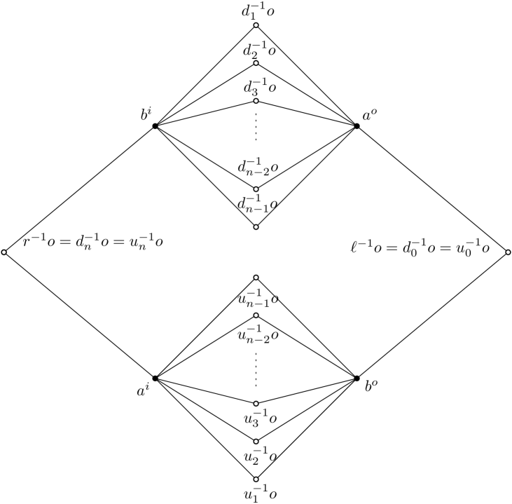
Figure 4. Edges of type I in the link of a real vertex.

Edges of type II in $\Lambda_{v}$ are edges between two fake vertices. They are characterized by Lemma 3.6. There do not exist edges of $\Lambda_{v}$ which are between two real vertices. We write $t\sim s$ (resp. $t\nsim s$) if vertices $t$ and $s$ are connected (resp. are not connected) by an edge.

Lemma 3.6.

1. $d^{-1}_{i}o\sim d^{-1}_{j}o$ if and only if $1\leq|j-i|\leq n-2$, in this case, the edge between $d^{-1}_{i}o$ and $d^{-1}_{j}o$ has angular length $=\frac{j-i}{2n}2\pi$. A similar statement holds with $d$ replaced by $u$.

2. If $1\leq i\leq n-1$ and $1\leq j\leq n-1$, then $d^{-1}_{i}o\nsim u^{-1}_{j}o$.

This lemma is deduced from the fact that $d^{-1}_{i}o\sim d^{-1}_{j}o$ if and only if $d^{-1}_{i}\Pi\cap d^{-1}_{j}\Pi$ has $\geq 2$ edges. We refer to [Artinmetric, Lemma 5.3] for a proof.

Now we study cycles in $\Lambda_{v}$. Let $\Lambda^{+}_{v}$ be the full subgraph of $\Lambda_{v}$ spanned by $\{b^{i},a^{o},d_{0}^{-1}o,d_{1}^{-1}o,\ldots,d_{n}^{-1}o\}$. Let $\Lambda^{-}_{v}$ be the full subgraph of $\Lambda_{v}$ spanned by $\{b^{o},a^{i},u_{0}^{-1}o,u_{1}^{-1}o,\ldots,u_{n}^{-1}o\}$.

Lemma 3.7.

[Artinmetric, Lemma 5.8] Suppose $\omega\subset\Lambda_{v}$ is a simple cycle. Then at least one of the following two situations happen:

1. $\omega\subset\Lambda^{+}_{v}$ or $\omega\subset\Lambda^{-}_{v}$;

2. $\ell^{-1}o\in\omega$ and $r^{-1}o\in\omega$.

Thus $\{\ell^{-1}o,r^{-1}o\}$ is called the necks of $\Lambda_{v}$. The next two lemmas give more detailed description of situations (1) and (2) of Lemma 3.7 respectively.

Lemma 3.8.

Suppose $\omega$ is a simple cycle in $\Lambda^{+}_{v}$ or $\Lambda^{-}_{v}$. Then $\omega$ is not $2$–full.

This follows from [Artinmetric, Lemma 5.6] and [Artinmetric, Lemma 5.7].

Lemma 3.9.

[Artinmetric, Lemma 5.11] Suppose $v$ is real and $\omega$ is an edge path from $r^{-1}o$ to $\ell^{-1}o$. Then $\omega$ has angular length $\geq\pi$.

If $\omega$ has angular length $=\pi$, then either $\omega\subset\Lambda^{+}_{v}$ or $\omega\subset\Lambda^{-}_{v}$, and the following are the only possibilities of $\omega$ when $\omega\subset\Lambda^{+}_{v}$:

1. $\omega=r^{-1}o\to b^{i}\to d^{-1}_{1}o\to d^{-1}_{0}o$;

2. $\omega=d^{-1}_{n}o\to d^{-1}_{n-1}o\to a^{o}\to\ell^{-1}o$;

3. $\omega=d^{-1}_{i_{1}}o\to d^{-1}_{i_{2}}o\to\cdots\to d^{-1}_{i_{k}}o$ where $n=i_{1}>i_{2}>\cdots>i_{k}=0$.

A similar statement holds for $\omega\subset\Lambda^{-}_{v}$.

Now we turn to the case when $v$ is a fake vertex. Up to the action of $DA_{n}$, we assume $v=o$. Vertices of $\Lambda_{v}$ consists of two classes. (1) Real vertices: these are the vertices in $\partial\Pi$. (2) Fake vertices: these are the fake vertices of cells $\Pi^{\prime}$ such that $\Pi^{\prime}\cap\Pi$ contain at least two edges.

By Lemma 3.1, $\Pi^{\prime}\cap\Pi$ is a connected path such that it contains exactly one of the tips of $\Pi$ and it is properly contained in a half of $\partial\Pi$. If $\Pi^{\prime}\cap\Pi$ is a path in the upper half (resp. lower half) of $\partial\Pi$ that has $m$ edges and contains the left tip, then we denote the fake vertex in $\Pi^{\prime}$ by $L_{m}$ (resp. $L^{\prime}_{m}$), and write $\Pi^{\prime}=\Pi_{L_{m}}$ (resp. $\Pi^{\prime}=\Pi_{L^{\prime}_{m}}$). Note that such $\Pi^{\prime}$ is unique by Lemma 3.2. Similarly, we define $R_{m}$, $R^{\prime}_{m}$, $\Pi_{R_{m}}$ and $\Pi_{R^{\prime}_{m}}$ respectively; see Figure 5.

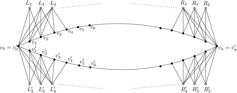
Figure 5. The link of a fake vertex.

The structure of $\Lambda_{v}$ will be easier to describe if we label vertices of $\partial\Pi$ differently as follows. The vertices in the upper half (resp. lower half) of $\partial\Pi$ are called $v_{0},v_{1},\ldots,v_{n}$ (resp. $v^{\prime}_{0},v^{\prime}_{1},\ldots,v^{\prime}_{n}$) from left to right. Note that $v_{0}=v^{\prime}_{0}$ and $v_{n}=v^{\prime}_{n}$.

Edges of $\Lambda_{v}$ consist of three classes:

1. Edges of type I. They are edges between real vertices of $\Lambda_{v}$. Hence they are edges in $\partial\Pi$. Each of them has angular length $=\frac{1}{2n}2\pi$.

2. Edges of type II. They are edges between a real vertex and a fake vertex, and they are characterized by Lemma 3.10 below.

3. Edges of type III. They are edges between fake vertices of $\Lambda_{v}$. We will not need information about them in this paper. The interested reader can find a description of them in [Artinmetric, Lemma 5.13].

We refer to Figure 5 for a picture of $\Lambda_{v}$. Edges of type I and some edges of type II are drawn. Edges of type III are not drawn in the picture.

Lemma 3.10.

1. The collection of vertices in $\partial\Pi$ adjacent to $L_{i}$ (resp. $L^{\prime}_{i}$) is $\{v_{0},v_{1},\ldots,\\ v_{i}\}$ (resp. $\{v^{\prime}_{0},v^{\prime}_{1},\ldots,v^{\prime}_{i}\}$).

2. The collection of vertices in $\partial\Pi$ adjacent to $R_{i}$ (resp. $R^{\prime}_{i}$) is $\{v_{n},v_{n-1},\\ \ldots,v_{n-i}\}$ (resp. $\{v^{\prime}_{n},v^{\prime}_{n-1},\ldots,v^{\prime}_{n-i}\}$).

3. The angular length of any edge between $L_{i}$ and a real vertex of $\Lambda_{v}$ is $\frac{i}{4n}2\pi$. The same holds with $L_{i}$ replaced by $L^{\prime}_{i},R_{i}$ and $R^{\prime}_{i}$.

Here (1) and (2) follow from the definition of $L_{i}$ and $R_{i}$. (3) follows from Definition 3.4.

Let $\Lambda^{+}_{v}$ be the full subgraph of $\Lambda_{v}$ spanned by

$$\{v_{0},v_{1},\ldots,v_{n}\}\cup\{L_{2},L_{3},\ldots,L_{n-1}\}\cup\{R_{2},R_{3},\ldots,R_{n-1}\}.$$

Let $\Lambda^{-}_{v}$ be the full subgraph of $\Lambda_{v}$ spanned by

$$\{v^{\prime}_{0},v^{\prime}_{1},\ldots,v^{\prime}_{n}\}\cup\{L^{\prime}_{2},L^{\prime}_{3},\ldots,L^{\prime}_{n-1}\}\cup\{R^{\prime}_{2},R^{\prime}_{3},\ldots,R^{\prime}_{n-1}\}.$$

The following is proved in [Artinmetric, Lemma 5.15] and [Artinmetric, Lemma 5.16]. It says that Lemma 3.7 and Lemma 3.8 continue to hold also in the case of $v$ being fake ($r^{-1}o$ and $\ell^{-1}o$ in the statement of Lemma 3.7 should be replaced by $v_{0}$ and $v_{n}$).

Lemma 3.11.

Suppose $\omega\subset\Lambda_{v}$ is a simple cycle. Then at least one of the following two situations happen:

1. $\omega\subset\Lambda^{+}_{v}$ or $\omega\subset\Lambda^{-}_{v}$;

2. $v_{0},v_{n}\in\omega$.

If $\omega$ is a simple cycle in $\Lambda^{+}_{v}$ or $\Lambda^{-}_{v}$ then $\omega$ is not $2$–full.

We call $\{v_{0},v_{n}\}$ the necks of $\Lambda_{v}$. The following is parallel to Lemma 3.9.

Lemma 3.12.

[Artinmetric, Lemma 5.18] Suppose $v$ is fake and $\omega$ is an edge path in $\Lambda_{v}$ from $v_{0}$ to $v_{n}$. Then $\omega$ has angular length $\geq\pi$.

If $\omega$ has angular length $=\pi$, then either $\omega\subset\Lambda^{+}_{v}$ or $\omega\subset\Lambda^{-}_{v}$, and the following are the only possibilities of $\omega$ when $\omega\subset\Lambda^{+}_{v}$:

1. $\omega$ does not contain fake vertices, i.e. $\omega=v_{0}\to v_{1}\to\cdots\to v_{n}$;

2. $\omega=v_{0}\to v_{1}\to\cdots\to v_{n-i_{1}}\to R_{i_{1}}\to\cdots\to R_{i_{m}}\to v_{n}$, where $i_{1}>\cdots>i_{m}\geq 2$;

3. $\omega=v_{0}\to L_{i_{1}}\to\cdots\to L_{i_{m}}\to v_{i_{m}}\to v_{i_{m}+1}\to\cdots\to v_{n}$, where $2\leq i_{1}<\cdots<i_{m}$;

4. $\omega=v_{0}\to L_{i_{1}}\to\cdots\to L_{i_{m}}\to v_{i_{m}}\to v_{i_{m+1}}\to\cdots\to v_{n-i^{\prime}_{1}}\to R_{i^{\prime}_{1}}\to\cdots\to R_{i^{\prime}_{m^{\prime}}}\to v_{n}$, where $2\leq i_{1}<\cdots<i_{m}$, $i^{\prime}_{1}>\cdots>i^{\prime}_{m^{\prime}}\geq 2$, and $i_{m}\leq n-i^{\prime}_{1}$.

A similar statement holds when $\omega\subset\Lambda^{-}_{v}$.

Remark 3.13.

Note that in all the cases (1)–(4) of Lemma 3.12, for any two non-neck vertices $u_{1},u_{2}\in\omega$ with $u_{1}$ real and $u_{2}$ fake, either $u_{1}$ is a tip of the cell $\Pi_{u_{2}}$ that contains $u_{2}$, or $u_{1}\notin\Pi_{u_{2}}$. This statement can be deduced from Lemma 3.10 and Lemma 3.1.

It follows from Lemma 3.7, Lemma 3.8, Lemma 3.9, Lemma 3.11 and Lemma 3.12 that $X_{n}$ is locally $2\pi$–large (cf. Definition 2.2). Moreover, we showed in [Artinmetric, Lemma 6.4] that $X_{n}$ is simply-connected.

Theorem 3.14.

$X_{n}$ is metrically systolic.

3.3. Flat vertices in disc diagrams over $X_{n}$

In this subsection, we explore links of certain flat vertices in reduced disc diagrams.

Definition 3.15.

A flat interior vertex in a disc diagram whose all neighbours are flat interior vertices is called a deep flat vertex.

Lemma 3.16.

Suppose $q^{\prime}\colon Y\to X_{n}$ satisfies all the conditions in Theorem 2.7. Let $y\in Y$ be a flat interior vertex and let $v=q^{\prime}(y)$. Then $q^{\prime}(\operatorname{lk}(y,Y))$ is a simple cycle in $\Lambda_{v}$ that is made of two paths of angular length $=\pi$ connecting the two necks of $\Lambda_{v}$, one in $\Lambda^{+}_{v}$ and one in $\Lambda^{-}_{v}$.

Proof.

Since $q^{\prime}$ is injective on $\operatorname{St}(y,Y)$, to simplify notation, we identify $\operatorname{lk}(y,Y)$ and $q^{\prime}(\operatorname{lk}(y,Y))$. By Lemma 3.7, Lemma 3.9 and Lemma 3.12, it suffices to rule out the cases $\operatorname{lk}(y,Y)\subset\Lambda^{+}_{v}$ and $\operatorname{lk}(y,Y)\subset\Lambda^{-}_{v}$. To rule out the former case, note that $\operatorname{lk}(y,Y)$ is a simple cycle in $\Lambda^{+}_{v}$, then by Lemma 3.8 (or Lemma 3.11), we can add a local diagonal to $\operatorname{lk}(y,Y)$ to cut it into a triangle and a cycle $\sigma$ with smaller number of edges. Now we apply same procedure to $\sigma$ (note that $\sigma\subset\Lambda^{+}_{v}$ since $\Lambda^{+}_{v}$ is a full subgraph of $\Lambda_{v}$ by definition). By repeating this process finitely many times, we know that $\operatorname{lk}(y,Y)$ bounds a disc diagram without interior vertices, which contradicts Theorem 2.7 (4). Similarly, we rule out the case $\operatorname{lk}(y,Y)\subset\Lambda^{-}_{v}$. ∎

Lemma 3.17.

Suppose $q^{\prime}\colon Y\to X_{n}$ satisfies all the conditions in Theorem 2.7. Let $v\in Y$ be a deep flat vertex. Then there do not exist two adjacent non-neck fake vertices in $q^{\prime}(\operatorname{lk}(v,Y))$.

To simply notation, denote $q^{\prime}(v)$ by $v$ and identify $\operatorname{lk}(v,Y)$ and $q^{\prime}(\operatorname{lk}(v,Y))$.

Proof.

Arguing by contradiction we assume there are two adjacent non-neck fake vertices $o_{1},o_{2}$ in $\operatorname{lk}(v,Y)$. We assume that $v=o$ when $v$ is fake (recall that $o$ is the fake vertex in the base cell $\Pi$), and $v=\ell$ when $v$ is real. For $i=1,2$, let $\Pi_{i}$ be the cell containing $o_{i}$.

Case 1: $v=\ell$. By Lemma 3.16, $\operatorname{lk}(v,Y)$ consists of two paths $\sigma_{1},\sigma_{2}$ of angular length $=\pi$ connecting the two necks of $\Lambda_{v}$. By Lemma 3.9, we can assume that $o_{1},o_{2}\in\sigma_{1}\subset\Lambda^{+}_{v}$. Then $\sigma_{1}$ must satisfy Lemma 3.9 (3), moreover, we can assume $d_{i_{2}}^{-1}o=o_{1}$ and $d_{i_{3}}^{-1}o=o_{2}$. See Figure 6.

Figure 6.

Now we consider the path $P=r^{-1}o\to v\to o_{2}$ in $\operatorname{lk}(o_{1},Y)$. Since $v$ is not a tip of $\Pi_{1}$, $v$ is not a neck of $\Lambda_{o_{1}}$. By Lemma 3.16, there is a path $\sigma$ of angular length $=\pi$ connecting the two necks of $\Lambda_{o_{1}}$ such that $P\subset\sigma\subset\operatorname{lk}(o_{1},Y)$. Since $P$ has a real vertex between two fake vertices, $\sigma$ satisfies Lemma 3.12 (4). It follows from Lemma 3.1 that $r^{-1}\Pi\cap\Pi_{1}\cap\Pi_{2}$ contains at least one edge. However, by Lemma 3.10, in case (4) of Lemma 3.12, $\Pi_{L_{i_{m}}}\cap\Pi\cap\Pi_{R_{i^{\prime}_{1}}}$ is either empty (when $i_{m}<n-i^{\prime}_{1}$) or one point (when $i_{m}=n-i^{\prime}_{1}$). This leads to a contradiction.

Case 2: $v=o$. By Lemma 3.16, $o_{1}$ and $o_{2}$ are consecutive non-neck fake vertices in a path of angular length $\pi$ between the two necks of $\Lambda_{o}$. By Lemma 3.12, we can assume either $o_{1}=L_{i_{1}}$, $o_{2}=L_{i_{2}}$, or $o_{1}=R_{i^{\prime}_{m^{\prime}-1}}$, $o_{2}=R_{i^{\prime}_{m^{\prime}}}$. Now we study the former case. See Figure 7.

Figure 7.

Consider the path $P=\ell\to o\to o_{2}$ in $\operatorname{lk}(o_{1},Y)$. Since $\ell$ is not a tip of $\Pi_{1}$, $\ell$ is not a neck of $\Lambda_{o_{1}}$. It follows that $P$ is contained in a path $\sigma\subset\Lambda_{o_{1}}$ of angular length $=\pi$ connecting the two necks of $\Lambda_{o_{1}}$. Note that $\ell\in\Pi_{2}$, but $\ell$ is not a tip of $\Pi_{2}$ (by applying Lemma 3.1 (3) to $\Pi_{2}\cap\Pi$). This contradicts Remark 3.13. The case $o_{1}=R_{i^{\prime}_{m^{\prime}-1}}$ and $o_{2}=R_{i^{\prime}_{m^{\prime}}}$ can be treated similarly. ∎

4. Local structure of quasi-Euclidean diagrams

In this section we recall the construction of the metrically systolic complexes for two-dimensional Artin groups, and use these complexes as a tool to study the local structure of quasi-Euclidean diagrams over the universal covers of standard presentation complexes of two-dimensional Artin groups.

4.1. The complex for $2$–dimensional Artin groups

Let $A_{\Gamma}$ be an Artin group with defining graph $\Gamma$. Let $\Gamma^{\prime}\subset\Gamma$ be a full subgraph with induced edge labeling and let $A_{\Gamma^{\prime}}$ be the Artin group with defining graph $\Gamma^{\prime}$. Then there is a natural homomorphism $A_{\Gamma^{\prime}}\to A_{\Gamma}$. By [lek], this homomorphism is injective. Subgroups of $A_{\Gamma}$ of the form $A_{\Gamma^{\prime}}$ are called standard subgroups. Let $P_{\Gamma}$ be the standard presentation complex of $A_{\Gamma}$, and let $X^{\ast}_{\Gamma}$ be the universal cover of $P_{\Gamma}$. We orient each edge in $P_{\Gamma}$ and label each edge in $P_{\Gamma}$ by a generator of $A_{\Gamma}$. Thus edges of $X^{\ast}_{\Gamma}$ have induced orientation and labeling. There is a natural embedding $P_{\Gamma^{\prime}}\hookrightarrow P_{\Gamma}$. Since $A_{\Gamma^{\prime}}\to A_{\Gamma}$ is injective, $P_{\Gamma^{\prime}}\hookrightarrow P_{\Gamma}$ lifts to various embeddings $X^{\ast}_{\Gamma^{\prime}}\to X^{\ast}_{\Gamma}$. Subcomplexes of $X^{\ast}_{\Gamma}$ arising in such way are called standard subcomplexes.

A block of $X^{\ast}_{\Gamma}$ is a standard subcomplex which comes from an edge in $\Gamma$. This edge is called the defining edge of the block. Two blocks with the same defining edge are either disjoint, or identical. A block is large if the label of the corresponding edge is at least $3$.

We define precells of $X^{\ast}_{\Gamma}$ as in Section 3.1. Each precell is embedded. We subdivide each precell as in Section 3.1 to obtain a simplicial complex $X^{\scalebox{0.53}{$\triangle$}}_{\Gamma}$. Fake vertices and real vertices of $X^{\scalebox{0.53}{$\triangle$}}_{\Gamma}$ are defined in a similar way.

Within each block of $X^{\scalebox{0.53}{$\triangle$}}_{\Gamma}$, we add edges between fake vertices as in Section 3.1. Then we take the flag completion to obtain $X_{\Gamma}$. The action $A_{\Gamma}\curvearrowright X^{\scalebox{0.53}{$\triangle$}}_{\Gamma}$ extends to a simplicial action $A_{\Gamma}\curvearrowright X_{\Gamma}$, which is proper and cocompact. A block in $X_{\Gamma}$ is defined to be the full subcomplex spanned by vertices in a block of $X^{\scalebox{0.53}{$\triangle$}}_{\Gamma}$. Intersection of two different blocks of $X_{\Gamma}$ does not contain fake vertices. Pick a block $B^{\Delta}\subset X^{\scalebox{0.53}{$\triangle$}}_{\Gamma}$, and let $B\subset X_{\Gamma}$ be the block containing $B^{\Delta}$. Let $n$ be the label of the defining edge of $B^{\Delta}$. Then by [Artinmetric, Lemma 6.3], the natural isomorphism $B^{\Delta}\to X^{\scalebox{0.53}{$\triangle$}}_{n}$ extends to an isomorphism $B\to X_{n}$.

Next we assign lengths to edges of $X_{\Gamma}$. Let $B\subset X_{\Gamma}$ be a block and let $B\to X_{n}$ be the isomorphism in the previous paragraph. We first rescale the edge lengths of $X_{n}$ defined in Section 3.1 by a uniform factor such that any edge between two real vertices has length $=1$. Then we pull back these edge lengths to $B$ by the above isomorphism. We repeat this process for each block of $X_{\Gamma}$. Note that if an edge of $X_{\Gamma}$ belongs to two different blocks, then this edge is between two real vertices, hence it has a well-defined length (which is $1$). The action of $A_{\Gamma}$ preserves edge lengths.

Theorem 4.1.

[Artinmetric, Theorem 6.1] If $A_{\Gamma}$ has dimension $\leq 2$, then $X_{\Gamma}$ with its piecewise Euclidean structure is metrically systolic.

From now on we will assume $A_{\Gamma}$ has dimension $\leq 2$.

Now we consider local structure of $X_{\Gamma}$. If $v\in X_{\Gamma}$ is a fake vertex, then there is a unique block $B\ni v$. Moreover, $\operatorname{lk}(v,X^{(2)}_{\Gamma})=\operatorname{lk}(v,B^{(2)})$ by our construction, which reduces to discussion in Section 3.2. Links of real vertices are more complicated since they can travel through several blocks. However, cycles of angular length $\leq 2\pi$ in the link have a relatively simple characterization as follows.

Lemma 4.2.

[Artinmetric, Lemma 6.7] Let $v\in X_{\Gamma}$ be a real vertex and let $\omega$ be a simple cycle in $\operatorname{lk}(v,X^{(2)}_{\Gamma})$ with angular length $\leq 2\pi$ in the link of $v$. Then exactly one of the following four situations happens:

1. $\omega$ is contained in one block;

2. $\omega$ travels through two different blocks $B_{1}$ and $B_{2}$ such that their defining edges intersect in a vertex $a$, and $\omega$ has angular length $=\pi$ inside each block, moreover, there are exactly two vertices in $\omega\cap B_{1}\cap B_{2}$ and they corresponding to an incoming $a$–edge and an outgoing $a$–edge based at $v$;

3. $\omega$ travels through three blocks $B_{1},B_{2},B_{3}$ such that the defining edges of these blocks form a triangle $\triangle(abc)\subset\Gamma$ and $\frac{1}{n_{1}}+\frac{1}{n_{2}}+\frac{1}{n_{3}}=1$ where $n_{1}$, $n_{2}$ and $n_{3}$ are labels of the edges of this triangle, moreover, $\omega$ is a $6$–cycle with its vertices alternating between real and fake such that the three real vertices in $\omega$ correspond to an $a$–edge, a $b$–edge and a $c$–edge based at $v$;

4. $\omega$ travels through four blocks such that the defining edges of these blocks form a full $4$–cycle in $\Gamma$, moreover, $\omega$ is a $4$–cycle with one edge of angular length $\pi/2$ in each block.

Note that in cases (2), (3) and (4), $\omega$ actually has angular length $=2\pi$.

4.2. Classification of flat points in diagrams over $X_{\Gamma}$

Let $q^{\prime}\colon Q^{\prime}\to X_{\Gamma}$ be a map which satisfies all the requirements of Theorem 2.7. We study the local properties of $q^{\prime}$ and $Q^{\prime}$ in this subsection.

We define a partial retraction $\rho$ from $X^{(2)}_{\Gamma}$ (defined on its subset) to $X^{\scalebox{0.53}{$\triangle$}}_{\Gamma}$ as follows. The map is the identity on the $2$–skeleton of $X^{\scalebox{0.53}{$\triangle$}}_{\Gamma}$. Let $\overline{o_{1}o_{2}}$ be an edge of $X^{(2)}_{\Gamma}$ not in $X^{\scalebox{0.53}{$\triangle$}}_{\Gamma}$, where $o_{i}$ is the fake vertex in some cell $\Pi_{i}$ for $i=1,2$. Let $m$ be the middle point of $\partial\Pi_{1}\cap\partial\Pi_{2}$ and let $x_{1},x_{2}$ be the two endpoints of $\partial\Pi_{1}\cap\partial\Pi_{2}$. We map $\overline{o_{1}o_{2}}$ homeomorphically to the concatenation of $\overline{o_{1}m}$ and $\overline{mo_{2}}$, and map the triangle $\triangle(o_{1}o_{2}x_{1})$ (resp. $\triangle(o_{1}o_{2}x_{2})$) homeomorphically to the region in $\Pi_{1}\cup\Pi_{2}$ bounded by $\overline{o_{1}x_{1}}$, $\overline{x_{1}o_{2}}$, $\overline{o_{2}m}$ and $\overline{mo_{1}}$ (resp. $\overline{o_{1}x_{2}}$, $\overline{x_{2}o_{2}}$, $\overline{o_{2}m}$ and $\overline{mo_{1}}$). This finishes the definition of $\rho$. Note that $\rho$ is not defined on the whole space $X^{(2)}_{\Gamma}$. That is why we call it a partial retraction. More precisely, for a triangle $\Delta\subset X^{(2)}_{\Gamma}$, $\rho(\Delta)$ is defined if and only if $\Delta$ satisfies one of the following two cases:

1. $\Delta$ has two real vertices and one fake vertices, in this case $\rho(\Delta)=\Delta$;

2. $\Delta$ has one real vertex $v$ and two interior vertices $o_{1}$ and $o_{2}$, moreover, $v$ is a tip of $\Pi_{1}$ or $\Pi_{2}$, where $\Pi_{i}$ is the cell containing $o_{i}$ for $i=1,2$.

Lemma 4.3.

Let $q=\rho\circ q^{\prime}$. If $\Delta\subset Q^{\prime}$ is a triangle such that all of its vertices are flat and deep, then $q(\Delta)$ is defined.

Proof.

If all vertices of $q^{\prime}(\Delta)$ are fake, then for any vertex $x\in\Delta$, the cycle $q^{\prime}(\operatorname{lk}(x,Q^{\prime}))$ in $\operatorname{lk}(q^{\prime}(x),X^{(2)}_{\Gamma})$ contains two consecutive fake vertices, hence contradicts Lemma 3.17. If $q^{\prime}(\Delta)$ has one real vertex $u$ and two interior vertices $o_{1}$ and $o_{2}$, but $u$ is neither the tip of $\Pi_{1}$ nor the tip of $\Pi_{2}$ ($\Pi_{i}$ is the cell containing $o_{i}$), then $u\in\Pi_{1}$ and $u$ is not a neck of $\operatorname{lk}(o_{2},X^{(2)}_{\Gamma})$, which contradicts Remark 3.13 (let the non-neck real vertex and the fake vertex in Remark 3.13 be $u$ and $o_{1}$ respectively). ∎

In what follows we use the map $q$ as in Lemma 4.3 (wherever it is well-defined). A vertex $x\in Q^{\prime}$ is real or fake if $q^{\prime}(x)=q(x)$ is, respectively, real or fake.

Lemma 4.4.

Suppose $x\in Q^{\prime}$ is flat, deep and fake, then the restriction of $q$ to $\operatorname{St}(x,Q^{\prime})$ is an embedding. Moreover, $q(\operatorname{St}(x,Q^{\prime}))$ contains the cell of $X^{\scalebox{0.53}{$\triangle$}}_{\Gamma}$ containing $q(x)$.

Proof.

By Theorem 2.7, the restriction of $q^{\prime}$ to the closed star $\operatorname{St}(x,Q^{\prime})$ is an embedding. Let $v=q^{\prime}(x)$ and let $\omega=q^{\prime}(\operatorname{lk}(x,Q^{\prime}))$. Then

1. $\omega$ is a concatenation of two paths $\omega^{+}$ and $\omega^{-}$ such that each of them connects the two necks of $\Lambda_{v}=\operatorname{lk}(v,X^{(2)}_{\Gamma})$, and $\omega^{+}\subset\Lambda^{+}_{v}$, $\omega^{-}\subset\Lambda^{-}_{v}$;

2. $\omega^{+}$ and $\omega^{-}$ do not contain consecutive fake vertices.

(1) follows from Lemma 3.16, (2) follows from Lemma 3.17. By (2) and Lemma 3.12, there are only four possibilities for $\omega^{+}$:

1. $\omega^{+}$ does not contain fake vertices, i.e. $\omega=v_{0}\to v_{1}\to\cdots\to v_{n}$;

2. $\omega^{+}=v_{0}\to v_{1}\to\cdots\to v_{n-i}\to R_{i}\to v_{n}$, where $i\geq 2$;

3. $\omega^{+}=v_{0}\to L_{i}\to v_{i}\to v_{i+1}\to\cdots\to v_{n}$, where $2\leq i$;

4. $\omega^{+}=v_{0}\to L_{i}\to v_{i}\to v_{i+1}\to\cdots\to v_{n-j}\to R_{j}\to v_{n}$, where $2\leq i$, $j\geq 2$, and $i\leq n-j$.

A similar statement holds for $\omega^{-}$. Then the lemma follows from Lemma 3.10 and the definition of $\rho$ (see Figure 8 for an example). ∎

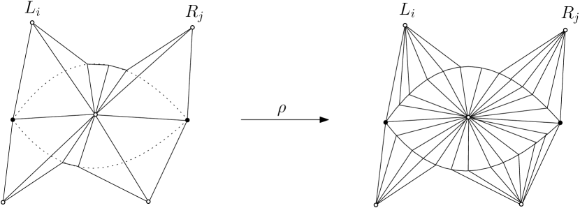
Figure 8.

Let $x$ be as in Lemma 4.4. Then for any fake vertex $x^{\prime}\in\operatorname{lk}(x,Q^{\prime})$, there are exactly two triangles in $\operatorname{St}(x,Q^{\prime})$ containing $x^{\prime}$. The union of these two triangles is called an ear of $\operatorname{St}(x,Q^{\prime})$. Note that $\operatorname{St}(x,Q^{\prime})$ can have at most four ears. By Lemma 4.4 again, there is a subset of $\operatorname{St}(x,Q^{\prime})$ which is mapped to the cell containing $q^{\prime}(x)$ homeomorphically by $q$. We denote this subset by $C_{x}$. Note that the boundary $\partial C_{x}$ cuts through the ears of $\operatorname{St}(x,Q^{\prime})$ and follows the edges in $\operatorname{lk}(x,Q^{\prime})$ that are between two real vertices.

Lemma 4.5.

Suppose $x\in Q^{\prime}$ is flat, deep and real. Let $v=q^{\prime}(x)$. Suppose the cycle $\omega=q^{\prime}(\operatorname{lk}(x,Q^{\prime}))$ in $\operatorname{lk}(v,X^{(2)}_{\Gamma})$ satisfies Lemma 4.2 (1), then the restriction of $q$ to $\operatorname{St}(x,Q^{\prime})$ is an embedding. Moreover, there are exactly four fake vertices in $\omega$, and the four cells containing these four fake vertices can be ordered as $\{\Pi_{i}\}_{i=1}^{4}$ such that (see Figure 9)

1. each $\Pi_{i}$ contains $v$, and $\Pi_{1},\Pi_{2},\Pi_{3},\Pi_{4}$ are in the same block;

2. $v$ is the right tip of $\Pi_{2}$ and is the left tip of $\Pi_{1}$;

3. $v$ is not a tip of $\Pi_{3}$ or $\Pi_{4}$;

4. each of $\Pi_{3}\cap\Pi_{2}$, $\Pi_{3}\cap\Pi_{1}$, $\Pi_{4}\cap\Pi_{2}$ and $\Pi_{4}\cap\Pi_{1}$ contains at least one edge, hence $\Pi_{i}\cap(\Pi_{1}\cup\Pi_{2})$ is a half of $\Pi_{i}$ for $i=3,4$ by Lemma 3.1;

5. if in addition each vertex in $\operatorname{lk}(x,Q^{\prime})$ is deep and flat, then $\operatorname{St}(x,Q^{\prime})$ is contained in $\cup_{i=1}^{4}C_{x_{i}}$, where $x_{i}$ is the fake vertex in $\operatorname{lk}(x,Q^{\prime})$ such that $q(x_{i})$ is the fake vertex in $\Pi_{i}$;

6. under the assumption of (5), $x\in C_{x_{i}}$ for each $i$.

Figure 9.

Proof.

Let $B$ be the block containing $\omega$. We argue as before to deduce $\omega$ is a concatenation of two paths $\sigma_{1}$ and $\sigma_{2}$ connecting two necks of $\operatorname{lk}(v,B^{(1)})$ such that each of them satisfies one of the three possibilities in Lemma 3.9. Moreover, by Lemma 3.17, $k=3$ in Lemma 3.9 (3). Thus there are four fake vertices in $\omega$. We can assume $\Pi_{1}=\Pi$ is the base cell of $X_{n}$. Then the conclusions (1)-(4) of the lemma follows by letting $\Pi_{2}=r^{-1}\Pi$, $\Pi_{3}=d_{i}^{-1}o$ and $\Pi_{4}=u_{j}^{-1}o$ for some $1\leq i,j\leq n-1$. For (5), it follows from our assumption that the link of each fake vertex in $\operatorname{lk}(x,Q^{\prime})$ is as described in the proof of Lemma 4.4. Thus (5) follows from the definition of $\rho$ and $C_{x_{i}}$. To see (6), note that for each $C_{x_{i}}$, $x$ is either a real vertex in an ear of $\operatorname{St}(x_{i},Q^{\prime})$, or $x$ is inside an edge of $\operatorname{lk}(x_{i},Q^{\prime})$ whose two end points are real. Thus $x\in C_{x_{i}}$. We refer to Figure 10 for a particular example. ∎

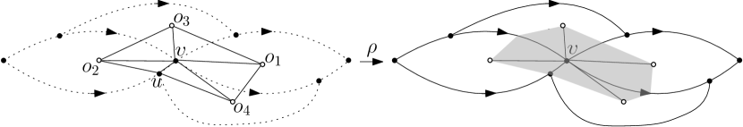
Figure 10. The path $o_{2}\to o_{3}\to o_{1}$ satisfies Lemma 3.9 (3), and the path $o_{2}\to u\to o_{4}\to o_{1}$ satisfies Lemma 3.9 (1).

Lemma 4.6.

Let $x,v,\omega$ be as in Lemma 4.5. If $\omega$ satisfies Lemma 4.2 (2), then the restriction of $q$ to $\operatorname{St}(x,Q^{\prime})$ is an embedding.

Let $\overline{ab},\overline{ac}\subset\Gamma$ be the defining edges of $B_{1}$ and $B_{2}$ as in Lemma 4.2 (2). For $i=1,2$, let the label of the defining edge of $B_{i}$ be $n_{i}$. Then there are exactly four fake vertices in $\omega$, and the four cells contains these four fake vertices can be ordered as $\{\Pi_{i}\}_{i=1}^{4}$ (see Figure 11) such that

1. each $\Pi_{i}$ contains $v$;

2. $\Pi_{1}$ and $\Pi_{2}$ are in $B_{1}$, and $\Pi_{3}$ and $\Pi_{4}$ are in $B_{2}$;

3. $\Pi_{1}\cap\Pi_{2}$ has $n_{1}-1$ edges, $\Pi_{3}\cap\Pi_{4}$ has $n_{2}-1$ edges, $\Pi_{1}\cap\Pi_{3}$ intersects along an $a$–edge, and $\Pi_{2}\cap\Pi_{4}$ intersects along an $a$–edge;

4. the analogous statements of Lemma 4.5 (5) and (6) hold.

Figure 11.

Remark 4.7.

We did not specify orientations of edges in Figure 11. However, it follows from Lemma 4.6 (3) that all vertical edges in Figure 11 have orientations pointing towards the same direction (all up or all down). All non-vertical edges in Figure 11 that are in $B_{1}$ have orientations pointing towards the same direction (all left or all right), and a similar statement holds with $B_{1}$ replaced by $B_{2}$.

Proof of Lemma 4.6.

We denote the two vertices in $\omega\cap B_{1}\cap B_{2}$ by $a^{i}$ and $a^{o}$ respectively. For $i=1,2$, let $\sigma_{i}$ be the sub-path of $\omega$ from $a^{o}$ to $a^{i}$ in $\operatorname{lk}(v,B^{(1)}_{i})$. We now study the possibilities for $\sigma_{1}$. We identify $B_{1}$ with $X_{n_{1}}$ and assume $v=\ell$ in the cell $\Pi$ of $X_{n_{1}}$.

By the discussion in Section 3.2, all edges of type II in $\operatorname{lk}(v,B^{(1)}_{1})$ (see Figure 4) are between two interior vertices, and there are no edges between real vertices. Thus to travel from one real vertex to another real vertex in $\operatorname{lk}(v,B^{(1)}_{1})$, one has to go through at least two edges of type I. However, only two edges of type I do not bring one from $a^{i}$ to $a^{o}$. So we need at least one another edge. By Lemma 3.6, an edge in $\operatorname{lk}(v,B^{(1)}_{1})$ has angular length at least $\frac{1}{2n}2\pi$. Thus $\sigma$ is made of two edges of type I and one edges of type II with minimal angular length. Thus $\sigma_{1}=a^{o}\to u_{0}^{-1}o\to u_{1}^{-1}o\to a^{i}$ or $\sigma_{1}=a^{o}\to d_{n_{1}-1}^{-1}o\to d_{n}^{-1}o\to a^{i}$. Note that $u_{0}^{-1}\Pi\cap u_{1}^{-1}\Pi$ has $n_{1}-1$ edges, and $d_{n-1}^{-1}\Pi\cap d_{n}^{-1}\Pi$ has $n_{1}-1$ edges (see Figure 12). A similar statement holds for $\sigma_{2}$. Now the lemma follows from the definition of $\rho$. ∎

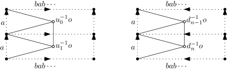
Figure 12.

Lemma 4.8.

Let $x,v,\omega$ be as in Lemma 4.5. If $\omega$ satisfies Lemma 4.2 (3), then the restriction of $q$ to $\operatorname{St}(x,Q^{\prime})$ is an embedding. Moreover, let $\{B_{i}\}_{i=1}^{3}$ be as in Lemma 4.2 (3). Then there are three cells $\{\Pi_{i}\subset B_{i}\}_{i=1}^{3}$ as in Figure 13 (left) such that

1. $v\in\Pi_{i}$ for $1\leq i\leq 3$;

2. each of $\Pi_{1}\cap\Pi_{2}$, $\Pi_{2}\cap\Pi_{3}$, and $\Pi_{3}\cap\Pi_{1}$ consists of one edge;

3. the analogous statements of Lemma 4.5 (5) and (6) hold.

A similar statement holds when $\omega$ satisfies Lemma 4.2 (4), where we have four squares around $v$, see Figure 13 right.

Figure 13.

Proof.

Take $\omega=\sigma_{1}\cup\sigma_{2}\cup\sigma_{3}$ where each $\sigma_{i}$ is a sub-path of $\omega$ made of two edges such that $\sigma_{i}\subset B_{i}$. For $1\leq i\leq 3$, we take $\Pi_{i}$ to be the cell that contains the fake vertex in $\sigma_{i}$. Then $\sigma_{i}\subset\Pi_{i}$. Thus $q^{\prime}(\operatorname{St}(x,Q^{\prime}))\subset X^{\scalebox{0.53}{$\triangle$}}_{\Gamma}$. Consequently, $\rho$ is the identity on $q^{\prime}(\operatorname{St}(x,Q^{\prime}))$. Hence the lemma follows. ∎

4.3. A new cell structure on the quasiflat

It follows from Lemma 4.3, Lemma 4.4, Lemma 4.5, Lemma 4.6 and Lemma 4.8 that if $x\in Q^{\prime}$ is flat and deep, then the restriction of $q$ to $\operatorname{St}(x,Q^{\prime})$ is well-defined (in particular, it is well-defined outside a compact set) and it is an embedding. Now we think of the range of $q$ as $X^{\ast}_{\Gamma}$. In this subsection we want to “pull back” the cell structure on $X^{\ast}_{\Gamma}$ to an appropriate subset of $Q^{\prime}$ via $q$.

Choose a base point $x_{0}\in Q^{\prime}$. For $R>0$, let $Q^{\prime}_{R}$ be the smallest subcomplex of $Q^{\prime}$ that contains $Q^{\prime}\setminus B(x_{0},R)$. Recall that $B(x_{0},R)$ is the ball of radius $R$ centered at $x_{0}$. Let $Q^{\prime}_{R^{+}}$ be the subcomplex made of all triangles of $Q^{\prime}$ which have non-trivial intersection with $Q^{\prime}_{R}$. By Theorem 2.7, we choose $R$ large enough such that each vertex in $Q$ that has combinatorial distance $\leq 5$ from $Q^{\prime}_{R^{+}}$ is flat and deep.

Lemma 4.9.

Suppose $C_{x_{1}}\cap C_{x_{2}}\neq\emptyset$ for two fake, deep and flat vertices $x_{1},x_{2}\in Q^{\prime}$. We also assume each vertex in $\operatorname{St}(x_{1},Q^{\prime})$ is flat and deep. Let $\Pi_{i}$ be the cell containing $o_{i}=q(x_{i})$. Then $q$ maps $C_{x_{1}}\cup C_{x_{2}}$ homeomorphically onto $\Pi_{1}\cup\Pi_{2}$. In particular, $C_{x_{1}}\cap C_{x_{2}}$ is a connected interval (possibly degenerate).

Proof.

Note that $x_{1}$ and $x_{2}$ have combinatorial distance $\leq 2$ in $Q^{\prime}$. We claim that if $x_{1}$ and $x_{2}$ are not adjacent, then $o_{1}$ and $o_{2}$ are not adjacent. To see this, note that there exists $x\in\operatorname{lk}(x_{1},Q^{\prime})$ such that $x_{1},x_{2}\in\operatorname{lk}(x,Q^{\prime})$. Since $x$ is deep and flat, the claim follows from the descriptions of $\operatorname{lk}(x,Q^{\prime})$ in Lemma 4.4, Lemma 4.5, Lemma 4.6 and Lemma 4.8.

If $x_{1}$ and $x_{2}$ are adjacent, then so are $o_{1}$ and $o_{2}$. It is clear that $q(C_{x_{1}}\cap C_{x_{2}})\subset\Pi_{1}\cap\Pi_{2}$. Let $\omega$ be the arc on $\partial C_{x_{1}}$ which is mapped homeomorphically to $\Pi_{1}\cap\Pi_{2}\subset\partial\Pi_{1}$. Then $C_{x_{1}}\cap C_{x_{2}}\subset\omega$ since $q|_{C_{x_{1}}}$ is an embedding. However, $\omega$ cuts through an ear of $\operatorname{St}(x_{1},Q^{\prime})$ thus, by definition of $C_{x_{i}}$, we have $\omega\subset C_{x_{1}}\cap C_{x_{2}}$. Hence $C_{x_{1}}\cap C_{x_{2}}=\omega$ and the lemma follows.

Suppose $x_{1}$ and $x_{2}$ are not adjacent. Since $C_{x_{1}}\cap C_{x_{2}}\neq\emptyset$, the intersection $\operatorname{St}(x_{1},Q^{\prime})\cap\operatorname{St}(x_{2},Q^{\prime})$ consists of at least one vertex. If there is a fake vertex $x\in\operatorname{St}(x_{1},Q^{\prime})\cap\operatorname{St}(x_{2},Q^{\prime})$, then let $\Pi_{x}$ be the cell containing $q(x)$. Since $x_{1}$ and $x_{2}$ are fake vertices in $\operatorname{lk}(x,Q^{\prime})$, by the description of $\operatorname{lk}(x,Q^{\prime})$ in Lemma 4.4, we know $\Pi_{1}\cap\Pi_{x}$ contains an edge, $\Pi_{2}\cap\Pi_{x}$ contains an edge and $(\Pi_{1}\cap\Pi_{x})\cap(\Pi_{2}\cap\Pi_{x})$ is at most one point. Thus $\Pi_{1}\cap\Pi_{2}$ is one point by Lemma 3.3 (note that $\Pi_{1},\Pi_{2}$ and $\Pi_{x}$ are in the same block). Thus the lemma follows by the discussion in the previous paragraph. Now suppose there are no fake vertices in $\operatorname{St}(x_{1},Q^{\prime})\cap\operatorname{St}(x_{2},Q^{\prime})$. If there is an edge $e$ in $\operatorname{St}(x_{1},Q^{\prime})\cap\operatorname{St}(x_{2},Q^{\prime})$, then $e\subset C_{x_{1}}\cap C_{x_{2}}$ since both endpoints of $e$ are real. Thus $q(e)$ is an edge in $\Pi_{1}\cap\Pi_{2}$. However, $\Pi_{1}\cap\Pi_{2}$ has at most one edge since $o_{1}$ and $o_{2}$ are not adjacent. Thus $e=C_{x_{1}}\cap C_{x_{2}}$ and the lemma follows. If there are no edges in $\operatorname{St}(x_{1},Q^{\prime})\cap\operatorname{St}(x_{2},Q^{\prime})$, then let $x$ be a vertex in this intersection. Since $x_{1}$ and $x_{2}$ are two fake vertices in $\operatorname{lk}(x,Q^{\prime})$, in all cases of Lemma 4.5, Lemma 4.6 and Lemma 4.8, $\Pi_{1}\cap\Pi_{2}$ is a point whenever $\operatorname{St}(x_{1},Q^{\prime})\cap\operatorname{St}(x_{2},Q^{\prime})$ is a real vertex. Hence the lemma follows. ∎

Lemma 4.10.

$Q^{\prime}_{R}$ is contained in the union of $C_{x}$ with $x$ varying among vertices of $Q^{\prime}_{R^{+}}$ that are flat, deep and fake.

Proof.

Recall that there are no triangles with three fake vertices in $X_{\Gamma}$, thus the same is true for $Q^{\prime}$. Thus $Q^{\prime}_{R}$ is contained in the union of $\operatorname{St}(x,Q^{\prime})$ with $x$ ranging over real vertices in $Q^{\prime}_{R}$. By Lemma 4.5, Lemma 4.6, Lemma 4.8 and our choice of $R$, for any real $x\in Q^{\prime}_{R}$, $\operatorname{St}(x,Q^{\prime})$ is contained in the union of $C_{y}$ with $y$ varying among fake vertices in $\operatorname{lk}(x,Q^{\prime})$. Note that $y\in Q^{\prime}_{R^{+}}$. Then the lemma follows. ∎

Let $Q_{R}$ be the union of $C_{x}$ with $x$ varying among fake vertices of $Q^{\prime}_{R^{+}}$. By Lemma 4.9 and Lemma 4.10, $Q_{R}$ has a well-defined cell structure whose closed $2$–cells are the $C_{x}$, and whose edges (resp. vertices) are arcs (resp. points) in the boundary of $C_{x}$ which are mapped to edges (resp. vertices) in $X^{\ast}_{\Gamma}$ by $q$. Also, Lemma 4.9 implies that we can pullback the orientation and labeling of edges of $X^{\ast}_{\Gamma}$ to orientation and labeling of edges of $Q_{R}$.

A vertex of $Q_{R}$ is interior if it has a neighborhood in $Q_{R}$ which is homeomorphic to an open disc. Let $\operatorname{St}(x,Q_{R})$ be the union of cells of $Q_{R}$ that contain $x$. Now we look at the structure of $\operatorname{St}(x,Q_{R})$.

Lemma 4.11.

Let $x\in Q_{R}$ be an interior vertex. Then the following are the only possibilities for $\operatorname{St}(x,Q_{R})$.

1. $\operatorname{St}(x,Q_{R})$ is a union of two $2$–cells.

2. The point $x$ corresponds to a real vertex in $Q^{\prime}$, and $q$ maps $\operatorname{St}(x,Q_{R})$ homeomorphically onto the union of the $\Pi_{i}$ in $X^{\ast}_{\Gamma}$ described in Lemma 4.5, Lemma 4.6, or Lemma 4.8.

Proof.

Suppose $x$ is not a real vertex of $Q^{\prime}$. There are at least two $2$–cells $C_{x_{1}}$, $C_{x_{2}}$ in $Q_{R}$ that contain $x$. Thus $x$ is in the interior of an ear of $\operatorname{St}(x_{i},Q^{\prime})$ for $i=1,2$. Hence $x_{1}$ and $x_{2}$ are adjacent in $Q^{\prime}$, and $\operatorname{St}(x_{1},Q^{\prime})$ and $\operatorname{St}(x_{2},Q^{\prime})$ share an ear. Now (1) follows.

Suppose $x$ is a real vertex of $Q^{\prime}$. Then each vertex of $\operatorname{St}(x,Q^{\prime})$ is flat and deep by our choice of $R$. If $x$ satisfies the assumptions of Lemma 4.5, then $\cup_{i=1}^{4}C_{x_{i}}\subset\operatorname{St}(x,Q^{\prime})$, by Lemma 4.5 (6). By Lemma 4.5 (5), $\cup_{i=1}^{4}C_{x_{i}}$ contains a disc neighborhood of $x$, thus $\cup_{i=1}^{4}C_{x_{i}}=\operatorname{St}(x,Q^{\prime})$. Since, by Lemma 4.9, $q$ maps $C_{x_{i}}\cup C_{x_{j}}$ homeomorphically onto $\Pi_{i}\cup\Pi_{j}$, $q$ maps $\cup_{i=1}^{4}C_{x_{i}}$ homeomorphically onto $\cup_{i=1}^{4}\Pi_{i}$. The cases of Lemma 4.6 and Lemma 4.8 are similar. ∎

Definition 4.12.

An interior vertex $v\in Q_{R}$ is of type O if it satisfies Lemma 4.11 (1), and is of type I, II, or III if it satisfies Lemma 4.5, Lemma 4.6, or Lemma 4.8, respectively. The support of a $2$–cell in $Q_{R}$ is the defining edge of the block of $X^{\ast}_{\Gamma}$ that contains the $q$–image of this $2$–cell. The support of a vertex of $Q_{R}$ is the union of the supports of $2$–cells in $Q_{R}$ that contain this vertex. For a type III vertex $v$, its support is either a triangle or a square, and $v$ is called either a $\triangle$–vertex or a $\square$–vertex, respectively. (See Table 1 on page 1.) By Lemma 4.2 (3) and (4), the Coxeter group whose defining graph is the support of $v$ acts on the Euclidean plane.

type O
type I
type II
type III $\triangle$–vertex
type III $\square$–vertex

Table 1. Types of flat vertices.

Note that $\operatorname{St}(v_{1},Q_{R})\cap\operatorname{St}(v_{2},Q_{R})$ contains two $2$–cells for two adjacent vertices $v_{1},v_{2}$ of type III, thus we have the following result.

Lemma 4.13.

If two vertices of type III of $Q_{R}$ are adjacent, then they have the same support.

Since $Q^{\prime}_{R}\subset Q_{R}$ by Lemma 4.10, we will assume the quasiflat is represented by $q\colon Q_{R}\to X^{\ast}_{\Gamma}$. Each $2$–cell in $Q_{R}$ corresponds to a fake vertex in $Q^{\prime}_{R}$, which is called the vertex dual to this $2$–cell.

5. Singular lines, singular rays and atomic sectors

Throughout this section $\Gamma$ will the defining graph of an Artin group $A_{\Gamma}$ with dimension $\leq 2$.

5.1. Singular lines and singular rays

Definition 5.1.

A diamond line is a locally injective cellular map $k\colon U\to X^{\ast}_{\Gamma}$ satisfying

1. $U=\cup_{i=-\infty}^{\infty}C_{i}$ such that each $C_{i}$ is a $2$–cell whose boundary is a $2n$–gon for $n\geq 3$, and each $C_{i}$ intersects $C_{i+1}$ and $C_{i-1}$ in opposite vertices (and has empty intersection with other $2$–cells), see Figure 14 for the $n=3$ case;

2. $k(U)$ is contained in a block;

3. $k(C_{i}\cap C_{i+1})$ is a tip of both $k(C_{i})$ and $k(C_{i+1})$.

We define a diamond ray in a similar way by replacing $\cup_{i=-\infty}^{\infty}C_{i}$ by $\cup_{i=0}^{\infty}C_{i}$.

Figure 14. A part of a diamond line.

Let $k,U$ be as in Definition 5.1 and let $\overline{ab}\subset\Gamma$ be the defining edge of the block containing $k(U)$. Then the two lines in the $1$–skeleton of $U$ corresponding to the bi-infinite alternating word $\cdots ababa\cdots$ are called the boundary lines of $U$.

Remark 5.2.

Roughly speaking, each diamond line corresponds to the centralizer of the stabilizer of the block of $X^{\ast}_{\Gamma}$ that contains this diamond line (note that the stabilizer of a block is a conjugate of the standard subgroup associated with the defining edge of this block).

Each diamond line is embedded and quasi-isometrically embedded in $X^{\ast}_{\Gamma}$. This is clear when $\Gamma$ is an edge, and the general case follows from a result by Charney and Paris [charney2014convexity, Theorem 1.2]. Note that each large block is a union of diamond lines.

Before we state the next definition, recall that each Coxeter group with defining graph $\Gamma$ gives rise to its Davis complex $\mathbb{D}_{\Gamma}$, whose $1$–skeleton is the Cayley graph of the associated Coxeter group with bigons collapsed to single edges. In particular, each edge of $\mathbb{D}_{\Gamma}$ is labeled by a vertex of $\Gamma$. A wall in $\mathbb{D}_{\Gamma}$ is the fixed point set of a reflection in the associated Coxeter group.

Definition 5.3.

Suppose the defining graph $\Gamma$ of the Artin group $A_{\Gamma}$ contains a triangle $\Delta\subset\Gamma$ such that the labels $m,n,r$ of the three sides of $\Delta$ satisfy $\frac{1}{m}+\frac{1}{n}+\frac{1}{r}=1$. Let $\mathbb{D}_{\Delta}$ be the Davis complex of the Coxeter group with the defining graph $\Delta$. Then $\mathbb{D}_{\Delta}$ is isometric to $\mathbb{E}^{2}$ and edges of $\mathbb{D}_{\Delta}$ are labeled by vertices of $\Delta$. Let $U$ be the carrier of a wall in $\mathbb{D}_{\Delta}$ (i.e. $U$ is the union of cells that intersect this wall). See Figure 15 for an example when $(m,n,r)=(2,3,6)$.

Figure 15. A part of a Coxeter line.

A Coxeter line of $X^{\ast}_{\Gamma}$ is a locally injective cellular map $k\colon U\to X^{\ast}_{\Gamma}$ such that

1. $k$ preserves the label of edges;

2. if we pull back the orientation of edges of $X^{\ast}_{\Gamma}$ to $U$, then there are no orientation reversing vertices in the boundary of $U$.

If we restrict $k$ to a subcomplex of $U$ homeomorphic to $[0,\infty)\times[0,1]$ (resp. $[0,k]\times[0,1]$), we obtain a Coxeter ray (resp. Coxeter segment).

Let $V$ be the carrier (in $\mathbb{D}_{\Delta}$) of the region bounded by two different parallel walls $\mathcal{W}_{1},\mathcal{W}_{2}$ in $\mathbb{D}_{\Delta}$. A thickened Coxeter line is a locally injective cellular map $k^{\prime}\colon V\to X^{\ast}_{\Gamma}$ such that $k^{\prime}$ preserves the label of edges and $k^{\prime}$ restricted to the carriers of $\mathcal{W}_{1}$ and $\mathcal{W}_{2}$ forms two Coxeter lines.

The maps $k$ and $k^{\prime}$ in Definition 5.3 are injective and they are quasi-isometric embeddings. This can be deduced by considering the quotient homomorphism from $A_{\Gamma}$ to the Coxeter group with the defining graph $\Gamma$.

For a set of vertices $V$ in $\Gamma$, let $V^{\perp}$ be the collection of vertices of $\Gamma$ that are adjacent to each element in $V$ along an edge labeled by $2$. If both $V\neq\emptyset$ and $V^{\perp}\neq\emptyset$, as $A_{\Gamma}$ is assumed to have dimension $\leq 2$, the subgroup of $A_{\Gamma}$ generated by $V^{\perp}$ has to be free, and so is the subgroup of $A_{\Gamma}$ generated by $V$. In particular, neither $V^{\perp}$ nor $V$ contain a pair of adjacent vertices of $\Gamma$.

Definition 5.4.

A plain line is a line $L$ in the $1$–skeleton of $X^{\ast}_{\Gamma}$ such that the collection $V_{L}$ of labels of edges satisfies either $V_{L}$ is a singleton or $V^{\perp}_{L}\neq\emptyset$. A plain ray is defined in a similar fashion. A plain line or ray is single-labeled if $V_{L}$ is a singleton. A plain ray is chromatic if $V_{r}$ is not a singleton for any sub-ray $r$ of this plain ray.

Let $U=\cup_{i=-\infty}^{\infty}C_{i}$ be a union of $2$–cells such that

1. $\partial C_{i}$ is a $2n$–gon for each $i$ ($n\geq 2$);

2. $C_{i}\cap C_{i-1}$ and $C_{i}\cap C_{i+1}$ are two disjoint connected paths in $\partial C_{i}$ and each of them has $n-1$ edges;

3. $C_{i}\cap C_{j}=\emptyset$ for $|i-j|\geq 2$.

A thickened plain line is a cellular embedding $k\colon U\to X^{\ast}_{\Gamma}$ such that $k$ restricted to the two boundary lines of $U$ are plain lines.

Again it follows from [charney2014convexity, Theorem 1.2] that each plain line is quasi-isometrically embedded for some uniform quasi-isometric constants independent of the plain line.

Definition 5.5.

A singular ray is either a diamond ray, or a Coxeter ray, or a plain ray. We define singular line analogously.

5.2. Flats, half-flats and sectors

Since the left action $A_{\Gamma}\curvearrowright X^{\ast}_{\Gamma}$ is simply transitive on the vertex set of $X^{\ast}_{\Gamma}$, we choose an identification between elements of $A_{\Gamma}$ and vertices of $X^{\ast}_{\Gamma}$.

Definition 5.6.

Let $L$ be a diamond line containing the identity element of $A_{\Gamma}$. A diamond-plain flat is a subcomplex of $X^{\ast}_{\Gamma}$ of the form $g\cup_{i=-\infty}^{\infty}a^{i}L$ or $g\cup_{i=-\infty}^{\infty}b^{i}L$, where $a$ and $b$ are the labels of edges in $L$, $a^{i}L$ means the left translation of $L$ under the group element $a^{i}$ and $g$ is an element in $A_{\Gamma}$. Note that each diamond-plain flat can be naturally realized as the image of a locally injective cellular map $f\colon U\to X^{\ast}_{\Gamma}$ where $U$ is a union of subcomplexes isomorphic to diamond lines; see Figure 16.

Figure 16. A part of a diamond-plain flat and a diamond-plain sector (shaded).

Lemma 5.7.

The map $f$ above is an embedding.

Proof.

Since the image of $f$ is contained in a block, it suffices to consider the case when $\Gamma$ is an edge. One can deduce the injectivity of $f$ from the solution of the word problem for spherical Artin groups [brieskorn1972artin, deligne]. Here we provide a geometric proof depending on a complex constructed by Jon McCammond [McCammond2010]. The construction of such complex was presented in the proof of [huang2015cocompactly, Theorem 5.1].

Suppose the edge of $\Gamma$ is labeled by $n$. Let $K_{n}$ be the cube complex described in the Figure 17 below.

Figure 17.

On the left we see part of the $1$–skeleton of $K_{n}$ consisting of three edges labelled by $a,b,t$, and the right side indicates how to attach a rectangle (subdivided into $n$ squares) along its boundary path $\underbrace{ab\dots}_{n}t^{-1}\underbrace{b^{-1}a^{-1}\dots}_{n}t^{-1}$. It is easy to check that the link of each of the two vertices in $K_{n}$ is isomorphic to the spherical join of two points with $n$ points, hence $K_{n}$ is nonpositively curved and its universal cover $\widetilde{K}_{n}$ is isometric to tree times $\mathbb{E}^{1}$. There is a homotopy equivalence $h\colon K_{n}\to P_{\Gamma}$ by collapsing the $t$–edge. This induces a map $\widetilde{K}_{n}\to X^{\ast}_{\Gamma}$. Note that $h$ gives a one to one correspondence between lifts of $t$–edges in $\widetilde{K}_{n}$ and vertices in $X^{\ast}_{\Gamma}$; as well as one to one correspondence between vertical flat strips in $\widetilde{K}_{n}$ and diamond lines in $X^{\ast}_{\Gamma}$. Now the lemma follows from the CAT(0) geometry on $\widetilde{K}_{n}$. ∎

Thus each diamond-plain flat $F$ is homeomorphic to $\mathbb{R}^{2}$. Moreover, there is a subgroup $A_{F}\leq A_{\Gamma}$ isomorphic to $\mathbb{Z}\oplus\mathbb{Z}$ acting cocompactly on $F$ (for example, when $F=\cup_{i=-\infty}^{\infty}a^{i}L$, then $A_{F}$ is generated by $a$ and the centralizer of the standard subgroup of $A_{\Gamma}$ generated by $a$ and $b$).

Definition 5.8.

Choose a diamond-plain flat $F$ and let $v\in F$ be a vertex of a diamond line $L$ in $F$ being the intersection of two $2$–cells of $L$. Let $L_{1}\subset L$ be a diamond ray based at $v$ and let $L_{2}\subset F$ be a plain ray based at $v$. Then the region in $F$ bounded by $L_{1}$ and $L_{2}$ (including $L_{1}$ and $L_{2}$) is called a diamond-plain sector; see Figure 16. $L_{1}$ and $L_{2}$ are called the boundary rays of the diamond-plain sector.

Definition 5.9.

Let $L\subset X^{\ast}_{\Gamma}$ be a Coxeter line containing the identity element of $A_{\Gamma}$ and let $e$ be the edge in $L$ such that $e$ is dual to the wall in $L$ and $e$ contains the identity element of $A_{\Gamma}$. Suppose the label of $e$ is $a$. Then a Coxeter-plain flat is a subcomplex of $X^{\ast}_{\Gamma}$ of the form $g\cup_{i=-\infty}^{\infty}a^{i}L$, where $g\in A_{\Gamma}$. Let $L^{\prime}\subset L$ be a Coxeter ray starting at the edge $e$. A Coxeter-plain sector is a subcomplex of $X^{\ast}_{\Gamma}$ of the form $g\cup_{i=0}^{\infty}a^{i}L^{\prime}$, where $g\in A_{\Gamma}$; see Figure 18. The Coxeter-plain sector has two boundary rays, one is $L^{\prime}$ and another one is the plain ray containing $e$.

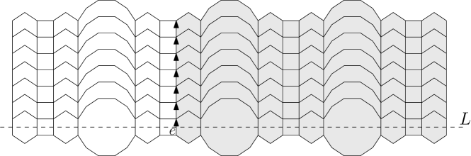
Figure 18. A part of a Coxeter-plain flat and a Coxeter-plain sector (shaded).

Since the Artin monoid injects into the Artin group by the work of Paris [paris2002artin], $L\cap a^{i}L=\emptyset$ for $i\geq 2$ and $L\cap aL$ is a boundary line of $L$. Thus each Coxeter-plain flat is a subcomplex of $X^{\ast}_{\Gamma}$ homeomorphic to $\mathbb{R}^{2}$.

Definition 5.10.

Let $\Delta$ and $\mathbb{D}_{\Delta}$ be as Definition 5.3. A Coxeter flat is a locally injective cellular map $f\colon\mathbb{D}_{\Delta}\to X^{\ast}_{\Gamma}$ such that

1. $f$ preserves the label of edges;

2. the orientation of edges in $\mathbb{D}_{\Delta}$ induced by $f$ satisfies the following: if two edges of $\mathbb{D}_{\Delta}$ are dual to parallel walls in $\mathbb{D}_{\Delta}$, then they are oriented towards the same direction.

By considering the $1$–Lipschitz quotient homomorphism from $A_{\Gamma}$ to the Coxeter group with defining graph $\Gamma$ as before (cf. the discussion after Definition 5.3), we know each Coxeter flat is embedded and quasi-isometrically embedded.

For each Coxeter flat $F$, there are exactly two families of parallel walls whose carriers in $F$ give rise to Coxeter lines. To see this, choose a $2$–cell $C\subset F$ with the maximal number of edges on its boundary and let $e_{1},e_{2}\subset\partial C$ be the two edges containing a tip $t\in\partial C$. Then by Definition 5.3 (2) and Definition 5.10 (2), the carrier of a wall $\mathcal{W}\subset F$ is a Coxeter line if and only if $\mathcal{W}$ is parallel to the wall of $F$ dual to $e_{1}$ or $e_{2}$.

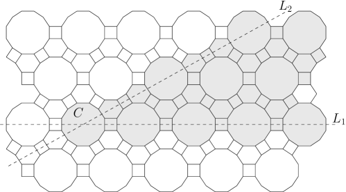
Figure 19. A part of a Coxeter flat and a Coxeter sector (shaded).

Definition 5.11.

Let $F$ be a Coxeter flat and choose two Coxeter lines $L_{1},L_{2}$ such that they intersect in a $2$–cell $C\in F$ (such Coxeter lines exists by the discussion in the previous paragraph). For $i=1,2$, let $L^{\prime}_{i}\subset L_{i}$ be a Coxeter ray starting at $C$. Then a Coxeter sector is defined to be the region in $F$ bounded by $L^{\prime}_{1}$ and $L^{\prime}_{2}$ (including $L^{\prime}_{1}$ and $L^{\prime}_{2}$); see Figure 19. $L^{\prime}_{1}$ and $L^{\prime}_{2}$ are called the boundary rays of the Coxeter sector.

Definition 5.12.

Let $Q$ be a quarter plane tiled by unit squares in a standard way. A plain sector is a locally injective cellular map $f\colon Q\to X^{\ast}_{\Gamma}$ such that $f$ restricted to the two boundary rays of $Q$ gives two plain rays.

For each plain sector, there is a full subgraph $\Gamma^{\prime}\subset\Gamma$ such that $Q$ is contained in a copy of $X^{\ast}_{\Gamma^{\prime}}$ inside $X^{\ast}_{\Gamma}$ and $A_{\Gamma^{\prime}}$ is a right-angled Artin group. Note that both $Q\to X^{\ast}_{\Gamma^{\prime}}$ and $X^{\ast}_{\Gamma^{\prime}}\to X^{\ast}_{\Gamma}$ are injective quasi-isometric embeddings (the first one follows from the fact that the Salvetti complexes of right-angled Artin groups are non-positively curved, and the second one follows from [charney2014convexity, Theorem 1.2]), thus $f$ is an injective quasi-isometric embedding.

Definition 5.13.

A diamond chromatic half-flat (DCH) is a locally injective cellular map $f\colon U=\cup_{i=1}^{\infty}L_{i}\to X^{\ast}_{\Gamma}$ such that

1. $f|_{L_{i}}$ is a diamond line for each $i$;

2. $L_{i}\cap L_{i+1}$ is a boundary line of both $L_{i}$ and $L_{i+1}$, moreover, $L_{i}\cap L_{j}=\emptyset$ for $|i-j|\geq 2$;

3. there does not exist $i_{0}\geq 1$ such that $f(\cup_{i=i_{0}}^{\infty}L_{i})$ is contained in a diamond-plain flat.

The boundary line of this DCH is defined to be the diamond line $f|_{L_{1}}$.

Figure 20. A part of a diamond chromatic half-flat (DCH).

By using the CAT(0) cube complex $\widetilde{K}_{n}$ in Lemma 5.7, one readily deduces that each DCH is embedded and quasi-isometrically embedded.

Definition 5.14.

A Coxeter chromatic half-flat (CCH) of type I is a locally injective cellular map $f\colon U=\cup_{i=1}^{\infty}L_{i}\to X^{\ast}_{\Gamma}$ such that

1. $f|_{L_{i}}$ is a thickened Coxeter line or a Coxeter line;

2. $L_{i}\cap L_{j}=\emptyset$ for $|i-j|\geq 2$;

3. $L_{i}\cap L_{i+1}$ is a boundary component of both $L_{i}$ and $L_{i+1}$, moreover, each vertex in $L_{i}\cap L_{i+1}$ is either of type O, or of type II (cf. Definition 4.12, and Table 1 on page 1);

4. there does not exist $i_{0}$ such that for all $i\geq i_{0}$, each vertex in $L_{i}\cap L_{i+1}$ is of type O; and there does not exist $i_{0}$ such that for all $i\geq i_{0}$, each vertex in $L_{i}\cap L_{i+1}$ is of type II.

The boundary line of this CCH is defined to be the Coxeter line containing $f|_{\partial U}$, where $\partial U$ is the boundary of $U$ in the topological sense.

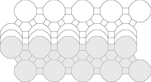
Figure 21. A part of a Coxeter chromatic half-flat (CCH) of type I. A thickened Coxeter line $L_{1}$ is shaded.

Definition 5.15.

Let $\Delta$ and $\mathbb{D}_{\Delta}$ be as Definition 5.3. Let $H$ be the carrier of a halfspace $\mathcal{H}\subset\mathbb{D}_{\Delta}$ bounded by a wall $\mathcal{W}_{1}$ of $\mathbb{D}_{\Delta}$. A Coxeter chromatic half-flat (CCH) of type II is a locally injective cellular map $f\colon H\to X^{\ast}_{\Gamma}$ satisfying all the following conditions:

1. $f$ preserves the label of edges;

2. $f$ restricted to the carrier of $\mathcal{W}_{1}$ is a Coxeter line;

3. there does not exist a halfspace $\mathcal{H}^{\prime}\subset\mathcal{H}$ such that the image of the carrier of $\mathcal{H}^{\prime}$ under $f$ is contained in a Coxeter flat; see Figure 22.

The boundary line of this CCH is the Coxeter line containing $f|_{\mathcal{W}_{1}}$.

Figure 22. A part of a Coxeter chromatic half-flat (CCH) of type II. The Carrier of $\mathcal{W}_{1}$ (shaded) is a Coxeter line. Orientations of edges along $L_{2}$ and $L_{3}$ are opposite.

As in the discussion after Definition 5.10, each CCH of type II is embedded and quasi-isometrically embedded.

Definition 5.16.

A plain chromatic half-flat (PCH) is a locally injective cellular map $f\colon U=\cup_{i=1}^{\infty}L_{i}\to X^{\ast}_{\Gamma}$ such that

1. $f|_{L_{i}}$ is a thickened plain line for each $i$;

2. $L_{i}\cap L_{j}=\emptyset$ for $|i-j|\geq 2$;

3. $L_{i}\cap L_{i+1}$ is a boundary line of both $L_{i}$ and $L_{i+1}$;

4. there does not exist $i_{0}\geq 1$ such that $f(\cup_{i=i_{0}}^{\infty}L_{i})$ is contained in a block;

5. there does not exist $i_{0}\geq 1$ such that $\cup_{i=i_{0}}^{\infty}L_{i}$ is made of squares.

Note that (5) implies that $f(\partial U)$ is a single-labeled plain line; see Figure 23. The boundary line of this PCH is $f|_{\partial U}$.

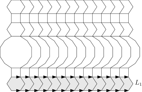
Figure 23. A part of a plain chromatic half-flat (PCH). A thickened plain line $L_{1}$ is shaded.

Definition 5.17.

An atomic sector is one of the objects among diamond-plain sector, Coxeter-plain sector, Coxeter sector, plain sector, DCH, CCH (of type I or II) and PCH. If $S$ is a DCH, CCH or PCH, then a boundary ray of $S$ is a singular ray contained in the boundary line of $S$.

For further reference, we collect all the types of atomic sectors in Table 2 on page 2.

One can build an atomic sector in a local and cell-by-cell fashion. There are plenty of atomic sectors in $X^{\ast}_{\Gamma}$. Actually, for any vertex in $X^{\ast}_{\Gamma}$, there is an atomic sector of given type whose image contains this vertex.

diamond-plain flat and sector
Coxeter-plain flat and sector
Coxeter flat and sector
diamond chromatic half-flat (DCH)
Coxeter chromatic half-flat (CCH) type I
Coxeter chromatic half-flat (CCH) type II
plain chromatic half-flat (PCH)

Table 2. Atomic sectors.

5.3. Properties of atomic sectors

For each Artin group $A_{\Gamma}$, Charney and Davis [CharneyDavis] defined an associated modified Deligne complex $D_{\Gamma}$. Now we recall their construction in the $2$–dimensional case, since it will be used for proving certain properties of atomic sectors. The vertex set $V$ of $D_{\Gamma}$ is in one to one correspondence with left cosets of the form $gA_{\Gamma^{\prime}}$, where $g\in A_{\Gamma}$ and $\Gamma^{\prime}$ is either the empty-subgraph of $\Gamma$ (in which case $A_{\Gamma^{\prime}}$ is the identity subgroup), or a vertex of $\Gamma$, or an edge of $\Gamma$. The rank of a vertex $gA_{\Gamma^{\prime}}$ of $V$ is the number of vertices in $\Gamma^{\prime}$. In other words, rank $2$ vertices of $V$ correspond to blocks of $X^{\ast}_{\Gamma}$, rank $1$ vertices of $V$ correspond to single-labeled plain lines in $X^{\ast}_{\Gamma}$, and rank $0$ vertices of $V$ correspond to vertices of $X^{\ast}_{\Gamma}$.

Note that $V$ has a partial order induced by inclusion of sets. A collection $\{v_{i}\}_{i=1}^{k}\subset V$ of vertices spans a $(k-1)$–dimensional simplex if $\{v_{i}\}_{i=1}^{k}$ form a chain with respect to the partial order. It is clear that $D_{\Gamma}$ is a $2$–dimensional simplicial complex, and $A_{\Gamma}$ acts on $D_{\Gamma}$ without inversions, i.e. if an element of $A_{\Gamma}$ fixes a simplex of $D_{\Gamma}$, then it fixes the simplex pointwise.

We endow $D_{\Gamma}$ with a piecewise Euclidean metric such that each triangle $\triangle(g_{1},g_{2}A_{s},g_{3}A_{\overline{st}})$ is a Euclidean triangle with angle $\pi/2$ at $g_{2}A_{s}$ and angle $\frac{\pi}{2n}$ at $g_{3}A_{\overline{st}}$ with $n$ being the label of the edge $\overline{st}$ of $\Gamma$. By [CharneyDavis, Proposition 4.4.5], $D_{\Gamma}$ is CAT(0) with such metric. As being observed in [MR2174269, Lemma 6], the action $A_{\Gamma}\curvearrowright D_{\Gamma}$ is semisimple.

Let $X^{b}_{\Gamma}$ be the barycentric subdivision of $X^{\ast}_{\Gamma}$. Then there is a simplicial map $\pi\colon X^{b}_{\Gamma}\to D_{\Gamma}$ which maps the center of each $2$–cell (resp. $1$–cell) in $X^{\ast}_{\Gamma}$ to the vertex in $D_{\Gamma}$ representing the block (resp. single-labeled plain line) of $X^{\ast}_{\Gamma}$ that contains this $2$–cell (resp. $1$–cell), and maps vertices of $X^{\ast}_{\Gamma}$ to the corresponding rank $0$ vertices in $D_{\Gamma}$.

Lemma 5.18.

If two different blocks $B$ and $B^{\prime}$ of $X^{\ast}_{\Gamma}$ satisfy that $B\cap B^{\prime}$ contains an edge, then $B\cap B^{\prime}$ is a single-labeled plain line.

Proof.

This follows from a more general fact by van der Lek [lek] that for any two full subgraphs $\Gamma_{1}$ and $\Gamma_{2}$ of $\Gamma$, we have $A_{\Gamma_{1}\cap\Gamma_{2}}=A_{\Gamma_{1}}\cap A_{\Gamma_{2}}$. ∎

Lemma 5.19.

Each atomic sector is embedded.

Proof.

It remains to prove the lemma for PCH and CCH of type I.

(PCH case.) Let $f\colon U=\cup_{i=1}^{\infty}L_{i}\to X^{\ast}_{\Gamma}$ be as in Definition 5.16. We group those consecutive $L_{i}$’s that are mapped by $f$ to the same block to form a new decomposition $U=\cup_{i=1}^{\infty}L^{\prime}_{i}$ so that the block $B_{i}$ containing $f(L^{\prime}_{i})$ satisfies $B_{i}\neq B_{i+1}$ for any $i\geq 1$. Each $B_{i}$ gives rise to a rank $2$ vertex in $D_{\Gamma}$, which we denote by $v_{i}$, and $B_{i}\cap B_{i+1}$ gives rise to a rank $1$ vertex in $D_{\Gamma}$ (cf. Lemma 5.18), which we denote by $w_{i}$. Then for each $i\geq 1$, $w_{i}$ is adjacent to $v_{i}$ and $v_{i+1}$ in $D_{\Gamma}$. Let $P\to D_{\Gamma}$ be the edge path starting from $v_{1}$ and traveling through $w_{1},v_{2},w_{2},v_{3},\ldots$. Note that $v_{i}\neq v_{i+1}$ (since $B_{i}\neq B_{i+1}$) and $w_{i}\neq w_{i+1}$ (since $f(L^{\prime}_{i+1})$ is embedded in $B_{i+1}$). Thus $P\to D_{\Gamma}$ is locally injective.

Let $g\in G$ be the generator of the stabilizer of $w_{1}$. Let $F_{g}$ be the fixed point set of $g$. Crisp [MR2174269] observed that $F_{g}$ is a tree. We repeat his argument here. Note that $F_{g}$ is a convex subcomplex of $D_{\Gamma}$. However, $g$ never fixes rank $0$ vertices, so $F_{g}$ lies in the part of the $1$–skeleton of $D_{\Gamma}$ which is spanned by rank $1$ and rank $2$ vertices. Thus $F_{g}$ is a tree.

Note that the edge path $P$ is actually contained in $F_{g}$. Since $P$ is locally injective, $P\to F_{g}$ is an embedding. Now we pick $i,j$ with $|i-j|\geq 2$. Then the segment of $P$ from $v_{i}$ from $v_{j}$ is a CAT(0) geodesic segment in $D_{\Gamma}$ made of $\geq 4$ edges thus, by the way we metrize $D_{\Gamma}$, there does not exist rank $0$ vertices which are adjacent to both $v_{i}$ and $v_{j}$. Also there are no rank $1$ vertices adjacent to both $v_{i}$ and $v_{j}$, since any such vertex has to be contained in $F_{g}$. Let $\pi\colon X^{b}_{\Gamma}\to D_{\Gamma}$ be the simplicial map defined as before. Note that each vertex in $\pi(B_{i})$ is adjacent to $v_{i}$. Thus $B_{i}\cap B_{j}=\emptyset$ whenever $|i-j|\geq 2$. From this, Lemma 5.18, and the fact that $f_{L^{\prime}_{i}}$ is injective for each $i$ we deduce that $f$ is injective.

(CCH of type I case.) Now let $f\colon U=\cup_{i=1}^{\infty}L_{i}\to X^{\ast}_{\Gamma}$ be as Definition 5.14. Walls in $U$ are defined to be the walls in the domains of Coxeter lines contained in $U$. If $\mathcal{W}\subset U$ is a wall, then $\pi(f(\mathcal{W}))$ is a geodesic line in the $1$–skeleton of $D_{\Gamma}$. We re-decompose $U$ as $U=\cup_{i=1}^{\infty}L^{\prime}_{i}$ such that

1. each $L^{\prime}_{i}$ is bounded by two walls;

2. either each vertex of $U$ in $L^{\prime}_{i}$ is of type III (we call such $L^{\prime}_{i}$ non-degenerate), or each vertex of $U$ in $L^{\prime}_{i}$ is of type O or type II (we call such $L^{\prime}_{i}$ degenerate);

3. $\{L^{\prime}_{i}\}_{i=1}^{\infty}$ alternates between non-degenerate and degenerate ones.

If $L^{\prime}_{i}$ is non-degenerate, then $\pi\circ f|_{L^{\prime}_{i}}$ is locally injective, hence injective by CAT(0) geometry. If $L^{\prime}_{i}$ is degenerate, then walls of $L^{\prime}_{i}$ are mapped by $\pi\circ f$ to the same geodesic line in $D_{\Gamma}$. Since each Coxeter line is periodic, pick an element $g\in A_{\Gamma}$ acting by translation on a Coxeter line $L\subset f(U)$. Note that $f(U)$ is invariant under the action of $g$. Moreover, let $\ell_{g}$ be the $\pi$–image of the wall in $L$, then $g$ acts by translation on $\ell_{g}$. Let $M_{g}$ be the collection of points in $D_{\Gamma}$ such that $d(x,gx)$ attains its minimum. Then $M_{g}$ admits a splitting $M_{g}=\ell_{g}\times T$ by [BridsonHaefliger1999, Theorem II.6.8]. Since $D_{\Gamma}$ is $2$–dimensional, $T$ is a tree. Note that $\pi\circ f(U)\subset M_{g}$. For each $i$, let $s_{i}\subset T$ be the orthogonal projection of $\pi\circ f(L^{\prime}_{i})$ onto the $T$–factor. If $L^{\prime}_{i}$ is non-degenerate, then $s_{i}$ is a segment with length $>0$. If $L^{\prime}_{i}$ is degenerate, then $s_{i}$ is a star shaped subset, i.e. $s_{i}$ is an union of segments along a vertex. We assume without loss of generality that $L^{\prime}_{1}$ is non-degenerate. Let $P\to T$ be the concatenation of $s_{2i+1}$ for $i\geq 0$ (note that the endpoint of $s_{2i-1}$ is the starting point of $s_{2i+1}$). By the argument in the PCH case, we know $f$ restricted to the carrier of $L^{\prime}_{i}$ in $U$ is injective for $i$ even. This implies that $P$ is locally injective at $s_{i}\cap s_{i+2}$ (for $i$ odd). Thus $P$ is an embedding. This and $f|_{L^{\prime}_{i}}$ being an embedding for each $i$ imply that $f$ is an embedding. ∎

Lemma 5.20.

Let $S_{1}$ and $S_{2}$ be two atomic sectors. If there is a sequence of $2$–dimensional discs $\{D_{i}\}_{i=1}^{\infty}\subset S_{1}\cap S_{2}$ such that $D_{i}$ contains a ball of radius $i$ in $S_{1}$ (with respect to the path metric on the $1$–skeleton of $S_{1}$), then $d_{H}(S_{1}\cap S_{2},S_{1})<\infty$ and $d_{H}(S_{1}\cap S_{2},S_{2})<\infty$. Moreover, $S_{1}$, $S_{2}$ and $S_{1}\cap S_{2}$ are atomic sectors of the same type.

Proof.

The lemma follows from a case by case inspection. Suppose $S_{1}$ and $S_{2}$ satisfy the assumption of the lemma. Let $D\subset S_{1}\cap S_{2}$ be a large disc. We only discuss the case when $S_{1}$ is a CCH of type I. Then other cases are either similar, or much simpler.

Let $S_{1}=\cup_{i=1}^{\infty}L^{\prime}_{i}$, $M_{g_{1}}=\ell_{g_{1}}\times T\subset D_{\Gamma}$ and the path $P\subset T$ be as in Lemma 5.19, where $g_{1}\in A_{\Gamma}$ is an element acting on $S_{1}$. Since a diamond-plain sector or a DCH is contained in a block, so $S_{2}$ can not be one of them. Also $S_{2}$ can not be a plain sector since a plain sector is made of squares. If $S_{2}$ is a PCH, then $D$ is contained in the carrier of $L^{\prime}_{i}$ (in $S_{1}$) for some $i$ even. Let $g_{2}\subset A_{\Gamma}$ be the element acting on $S_{2}$ and we define the tree $F_{g_{2}}$ as in Lemma 5.19. The existence of $D$ implies that a sub-segment of $F_{g_{2}}$ goes along the $\ell_{g}$ direction of $M_{g}$. The convexity of $F_{g_{2}}$ and $M_{g_{1}}$ implies that $F_{g_{2}}\cap M_{g_{2}}\subset\ell_{g}\times\{t\}$ for some $t\in T$. Since $\pi(S_{1})\subset M_{g_{2}}$ and each vertex of $\pi(S_{2})$ is either contained in $F_{g_{2}}$ or adjacent to a vertex in $F_{g_{2}}$, we know that $S_{1}\cap S_{2}$ is contained in the carrier of $L^{\prime}_{i}$ inside $S_{1}$. This rules out the possibility of $S_{2}$ being a PCH. The case of $S_{2}$ being a Coxeter-plain sector can be ruled out in a similar way. If $S_{2}$ is a Coxeter sector, then $D$ is contained in the carrier of $L^{\prime}_{i}$ (in $S_{1}$) for some $i$ odd and $\pi(S_{2})\subset M_{g_{1}}$. Note that $P$ and the projection of $\pi(S_{2})$ on $T$ are two rays which diverge from each other at some point, thus $S_{1}\cap S_{2}$ is contained in the carrier of $L^{\prime}_{i}$ inside $S_{1}$ for some odd $i$ and $S_{2}$ can not be a Coxeter sector.

Now suppose that $S_{2}$ is a CCH of type I or II and that $S_{2}$ is invariant under $g_{2}\in A_{\Gamma}$. The existence of $D$ implies that there is a Coxeter line $L\subset S_{2}$ such that $L\cap S_{1}$ contains a Coxeter segment $U$ (cf. Definition 5.3) which is sufficiently long. Thus we have the following two cases:

1. if $U$ is contained in a Coxeter line of $S_{1}$, then we know $L$ is a Coxeter line of $S_{1}$;

2. if $U$ is not contained in a Coxeter line of $S_{1}$, then $N$ is contained in a thickened Coxeter line of $S_{1}$, hence $L$ and a Coxeter line of $S_{1}$ span a Coxeter flat in $X^{\ast}_{\Gamma}$.

Let $\ell\subset D_{\Gamma}$ be the $\pi$–image of the wall in $L$. In both cases (1) and (2), we have $\ell\subset M_{g_{1}}$. If $\ell$ and $\ell_{g_{1}}$ are not parallel, then $P$ and the projection of $\ell$ on $T$ are two rays which diverge from each other at some point (since $\ell$ is periodic), which implies that $S_{1}\cap S_{2}$ is contained in the carrier of $L^{\prime}_{i}$ inside $S_{1}$ for some odd $i$. Thus $\ell$ and $\ell_{g_{1}}$ are parallel. Then $\pi(S_{2})\subset M_{g_{1}}$. The projections of $\pi(S_{1})$ and $\pi(S_{2})$ must contain a common geodesic ray, otherwise we can reach a contradiction as before. Now one readily deduces that $d_{H}(S_{1}\cap S_{2},S_{1})<\infty$ and $d_{H}(S_{1}\cap S_{2},S_{2})<\infty$. ∎

Now we recall the notion of locally finite homology. We use $\mathbb{Z}/2\mathbb{Z}$ coefficients throughout this paper. Recall that for a topological space $X$ we can consider locally finite chains in $X$, which are formal sums $\Sigma_{\lambda\in\Lambda}a_{\lambda}\sigma_{\lambda}$ where $a_{\lambda}\in\mathbb{Z}/2\mathbb{Z}$, $\sigma_{\lambda}$ are singular simplices, and any compact set in $X$ intersects the images of only finitely many $\sigma_{\lambda}$ with $a_{\lambda}\neq 0$. This gives rise to locally finite homology of $X$, denoted by $H^{\mathrm{lf}}_{*}(X)$. We define the relative locally finite homology $H^{\mathrm{lf}}_{*}(X,Y)$ for a subset $Y\subset X$ in a similar way. For a point $z\in Z\setminus Y$, there is a homomorphism $i\colon H^{\mathrm{lf}}_{k}(Z,Y)\to H^{\mathrm{lf}}_{k}(Z,Z\setminus\{z\})\cong H_{k}(Z,Z\setminus\{z\})$ induced by the inclusion of pairs $(Z,Y)\to(Z,Z-\{z\})$. For $[\sigma]\in H^{\mathrm{lf}}_{k}(Z,Y)$, we define the support set of $[\sigma]$, denoted $S_{[\sigma],Z,Y}$, to be $\{z\in Z\setminus Y\mid i_{\ast}[\sigma]\neq\textmd{Id}\}$. We will also use $S_{[\sigma]}$ to denote the support set if the underlying spaces $Z$ and $Y$ are clear.

Lemma 5.21.

Each atomic sector is quasi-isometrically embedded.

Proof.

The cases of diamond-plain sector, Coxeter-plain sector and Coxeter sector follow from the fact that any rank $2$ abelian subgroup of $A_{\Gamma}$ is quasi-isometrically embedded ([Artinmetric, Theorem 7.7]). The case of plain sector has already been discussed after Definition 5.12. It remains to consider chromatic half-flats. Let $U\subset X^{\ast}_{\Gamma}$ be a PCH and let $\{\ell_{i}\}_{i=1}^{\infty}$ be the collection of all plain lines in $U$ parallel to $\partial U$ such that $\ell_{1}=\partial U$ and $\ell_{i}$ is between $\ell_{i-1}$ and $\ell_{i+1}$. Since each $\ell_{i}$ is quasi-isometrically embedded with constants independent of $i$, it suffices to show that there is a constant $M$ such that $d_{A_{\Gamma}}(\ell_{i},\ell_{j})\geq M|i-j|$, where $d_{A_{\Gamma}}$ denotes the distance in the $1$–skeleton of $X^{\ast}_{\Gamma}$. Suppose the contrary holds. Then for any given $\epsilon>0$, there exists $\ell_{i},\ell_{j}$ such that $d_{A_{\Gamma}}(\ell_{i},\ell_{j})<\epsilon|i-j|$. Suppose $L=d_{A_{\Gamma}}(\ell_{i},\ell_{j})$. Then $|i-j|>L/\epsilon$. Let $P_{0}$ be a shortest edge path from a vertex $v_{0}\in\ell_{i}$ to a vertex $w_{0}\in\ell_{j}$. Let $g\in A_{\Gamma}$ be an element which translates $\ell_{i}$ by distance $L$. Let $C_{1}=v_{0}\to gv_{0}\to gw_{0}\to w_{0}\to v_{0}$ be the cycle traveling along $\ell_{i}$, $gP_{0}$, $\ell_{j}$ and $P_{0}$. Since $C_{1}$ has $\leq 4L$ edges and $A_{\Gamma}$ has quadratic Dehn function (by Corollary 2.4 and Theorem 4.1), there is a cellular $2$–chain $\sigma$ such that $\partial\sigma=C_{1}$, and $\sigma$ has at most $CL^{2}$ cells, where $C$ only depends on $A_{\Gamma}$. Since $\ell_{i}$ is quasi-isometrically embedded, $\alpha=\sum_{k=-\infty}^{\infty}g^{k}\sigma$ gives rise to a locally finite relative homology class $[\alpha]\in H^{\mathrm{lf}}_{2}(X^{\ast}_{\Gamma},\ell_{i}\cup\ell_{j})$. On the other hand, let $U_{ij}$ be the region of $U$ bounded by $\ell_{i}$ and $\ell_{j}$. The fundamental class of $U_{ij}$ gives another locally finite cellular chain $\beta$ such that $\partial\beta=\partial\alpha$. Then $[\beta]\in H^{\mathrm{lf}}_{2}(X^{\ast}_{\Gamma},\ell_{i}\cup\ell_{j})$ and $S_{[\beta]}=U_{ij}\setminus(\ell_{i}\cup\ell_{j})$. Note that $\alpha\cup\beta$ is a periodic “infinite cylinder”. Recall that $X^{\ast}_{\Gamma}$ is contractible by By [CharneyDavis, Theorem B] and [CharneyDavis, Corollary 1.4.2]. Then $X^{\ast}_{\Gamma}$ is also uniformly contractible since it is cocompact. Thus we can fill in the periodic infinite cylinder to obtain a locally finite singular $3$–chain $\gamma$ such that $\partial\gamma=\alpha-\beta$. Thus $[\alpha]=[\beta]$ and $S_{[\alpha]}=S_{[\beta]}=U_{ij}\setminus(\ell_{i}\cup\ell_{j})$. It is clear that $S_{[\alpha]}\subset\operatorname{Im}\alpha$, thus $U_{ij}\subset\operatorname{Im}\alpha$. Note that both $\operatorname{Im}\alpha$ and $U_{ij}$ are invariant under the action of the subgroup $\langle g\rangle\cong\mathbb{Z}$. Moreover, $\operatorname{Im}\alpha/\langle g\rangle$ has at most $CL^{2}$ $2$–cells, but $U_{ij}/\langle g\rangle$ has $L^{2}/\epsilon$ $2$–cells (since $|i-j|>L/\epsilon$). This will be contradictory to $U_{ij}\subset\operatorname{Im}\alpha$ if we take $\epsilon$ small enough. Similarly we deal with other chromatic half-flats, since they all have one periodic direction (the cases of DCH and CCH of type II have already been treated differently in Section 5.2). ∎

5.4. Completions of atomic sectors

A subset $A$ is coarsely contained in another subset $B$ of a metric space if $A$ is contained in the $R$–neighborhood of $B$ for some $R$. We say $A$ is the coarse intersection of a family of subsets $\{B_{i}\}_{i\in I}$ if there exists $R_{0}$ such that for all $R\geq R_{0}$, the Hausdorff distance between $A$ and $\cap_{i\in I}N_{R}(B_{i})$ is finite.

In the rest of this subsection, we define the completion of an atomic sector $S$, which (roughly speaking) is a “smallest possible subset” that is the coarse intersection of 2-dimensional quasiflats and coarsely contains $S$.

Lemma 5.22.

Let $S$ be an atomic sector which is not a plain sector or a diamond-plain sector. Then $S$ is a coarse intersection of finitely many $2$–dimensional quasiflats.

Proof.

Let $U=\cup_{i=1}^{\infty}L_{i}$ be a CCH of type I (see Table 2 on page 2). We assume without loss of generality that $L_{1}$ is a Coxeter line and $L_{2}$ is a thickened Coxeter line. Let $F$ be the Coxeter-plain flat containing $L_{1}$. Then the line $L_{1}\cap L_{2}$ divides $F$ into two half-spaces, which we denote by $U_{1}$ and $U_{2}$. Let $U_{3}=\cup_{i=2}^{\infty}L_{i}$. We glue $U_{1}$, $U_{2}$ and $U_{3}$ along $L_{1}\cap L_{2}$ to form a triplane $V$. Note that there is a locally injective map $V\to X^{\ast}_{\Gamma}$. By the same argument as in the proof of Lemma 5.19 and Lemma 5.21, we know that $U_{i}\cup U_{j}$ is embedded and quasi-isometrically embedded for any $1\leq i\neq j\leq 3$. Thus $U$ is the coarse intersection of the quasiflat $U_{3}\cup U_{1}$ and the quasiflat $U_{3}\cup U_{2}$. The case of CCH of type II is similar. If $U$ is a PCH, we can assume $L_{1}$ and $L_{2}$ are not in the same block. Let $F$ be the diamond flat containing $L_{1}$. Then we can form a triplane as before and find three quasiflats using the argument of Lemma 5.19 and Lemma 5.21. To deal with DCH, note that each DCH is contained in a large block. Then we can use the cube complex $\tilde{K}_{n}$ in Lemma 5.7 to conclude the proof.

If $S$ is a Coxeter sector, let $F$ be the Coxeter flat containing $S$. Let $L_{1}$ and $L_{2}$ be two Coxeter lines in $F$ that contains the two boundary rays of $S$. Then there are half-flats $H_{1}$ and $H_{2}$ of $F$ bounded by $L_{1}$ and $L_{2}$ respectively such that $S=H_{1}\cap H_{2}$. Since $F$ is quasi-isometrically embedded, $S$ is the coarse intersection of $H_{1}$ and $H_{2}$. However, each $H_{i}$ is the coarse intersection of two quasiflats by the argument in the previous paragraph. Thus we are done in the case of Coxeter sector. The case of Coxeter-plain sector is similar. ∎

We define the completion of an atomic sector which is not a plain sector or a diamond-plain sector to be itself. Before discussing completions of diamond-plain sectors and plain sectors, we need the following observation.

For two vertices $a,b\subset\Gamma$, we define $a\sim b$ if $a$ and $b$ are adjacent in $\Gamma$ along an edge labeled by an odd number. If $a\sim b$, then for each singled-labeled plain line $\ell_{a}$ in $X^{\ast}_{\Gamma}$ labeled by $a$, there is a thickened plain line $L$ such that

1. one boundary component of $L$ is $\ell_{a}$;

2. another boundary component of $L$ is a single-labeled plain line labeled by $b$.

Now we consider the equivalence relation on the vertex set of $\Gamma$ generated by $\sim$. Each equivalence class is called an odd component. Note that a plain line whose edges are labeled by an element in an odd component can be “parallelly transported” to a plain line with its edges labeled by another element in the same odd component via finitely many thickened plain lines.

If $S$ is a diamond-plain sector, let $F$ be the diamond flat containing $S$. Then $S$ is the intersection of two half-flats $H_{1},H_{2}$ of $F$ such that $H_{1}$ is bounded by a plain line $L_{1}$ and $H_{2}$ is bounded by a diamond line $L_{2}$. Note that $H_{2}$ is the coarse intersection of two 2-dimensional quasiflats. However, this may not be true for $H_{1}$ (e.g. when $\Gamma$ is an edge). Let $a\in\Gamma$ be the vertex corresponding to the label of edges in $L_{1}$. If every vertex in the odd component containing $a$ is a leaf in $\Gamma$ (recall that a leaf in a graph is a vertex which is only adjacent to one another vertex), then we define the completion of $S$ to be $H_{2}$. Observe that in this case either $a$ is a leaf in $\Gamma$ contained in an edge with an even label, or the component of $a$ in $\Gamma$ is an edge (with an odd label). If there exists a vertex $c$ in the odd component containing $a$ which is not a leaf, then the completion of $S$ is defined to be itself. In this case, we can form a triplane containing $H_{1}$, hence $H_{1}$ is the coarse intersection of two quasiflats and $S$ is the coarse intersection of finitely many quasiflats.

Now suppose $S$ is a plain sector. We write $S=r_{1}\times r_{2}$ where $r_{1}$ and $r_{2}$ are two boundary rays of $S$. For $i=1,2$, let $V_{i}\subset\Gamma$ be the collection of labels of edges in $r_{i}$. Let $V^{\perp}_{i}$ be the collection of vertices in $\Gamma$ which are adjacent to each vertex in $V_{i}$ along an edge labeled by $2$. The set $V_{i}$ is good if either $V^{\perp}_{i}$ has $\geq 2$ vertices, or $V_{i}$ is a singleton and there exists a non-leaf vertex in the odd component containing $V_{i}$. Since $V_{1}$ and $V_{2}$ form a join subgraph $\Gamma^{\prime}\subset\Gamma$, the latter case is equivalent to $V_{i}$ being a singleton and not a leaf.

If both $V_{1}$ and $V_{2}$ are good, then the completion of $S$ is $S$ itself. In this case, $S$ is the coarse intersection of finitely many $2$–dimensional quasiflats. Now we prove this statement. Note that $A_{\Gamma^{\prime}}$ is a right-angled Artin group. We assume $S$ is contained in a copy of $X^{\ast}_{\Gamma^{\prime}}$ in $X^{\ast}_{\Gamma}$. Then there is a flat $F=\ell_{1}\times\ell_{2}$ in $X^{\ast}_{\Gamma^{\prime}}$ such that $\ell_{i}$ is a geodesic line extending $r_{i}$ (such extension may not be unique). We know $S=H_{1}\cap H_{2}$ where $H_{i}$ is a half-flat in $F$ bounded by $\ell_{i}$. Since $F$ is isometrically embedded in $X^{\ast}_{\Gamma^{\prime}}$ and $X^{\ast}_{\Gamma^{\prime}}$ is quasi-isometrically embedded in $X^{\ast}_{\Gamma}$ ([charney2014convexity, Theorem 1.2]), we know $S$ is the coarse intersection of $H_{1}$ and $H_{2}$. Note that the labels of edges in $\ell_{i}$ are in $V_{i}$, then we deduce from the fact that $V_{1}$ and $V_{2}$ are good that each of $H_{1}$ and $H_{2}$ ia a coarse intersection of two quasiflats.

If only one of $V_{1},V_{2}$ is good, then $S$ is contained in a canonical half-flat $H$ such that $H$ is made of squares and $H$ is a coarse intersection of two quasiflats. Note that the boundary of $H$ is a single-labeled plain line. $H$ is defined to be the completion of $S$.

If both $V_{1}$ and $V_{2}$ are not good, then $V_{1}$ and $V_{2}$ are singletons. We extend $r_{i}$ to a single-labeled plain line $\ell_{i}$ and define the completion of $S$ to be the flat of the form $\ell_{1}\times\ell_{2}$.

Corollary 5.23.

For any atomic sector $S$, the completion $\bar{S}$ of $S$ is a coarse intersection of finitely many $2$–dimensional quasiflats.

6. Half Coxeter regions in $Q^{\prime}$ and $Q_{R}$

Let $x\in Q_{R}$ be a vertex of type III (see Table 1 on page 1). Let $K_{x}\subset Q^{\prime}$ be the convex hull of fake vertices of $Q^{\prime}$ that are dual to $2$–cells in $\operatorname{St}(x,Q_{R})$. Such $K_{x}$ is called a chamber or an $x$–chamber. Note that $K_{x}$ is either a triangle or a square, and define edges and vertices of $K_{x}$ with respect to the standard cell structure on a triangle or a square. $K_{x}$ is isometric to the standard fundamental domain of the action of a Euclidean Coxeter group on $\mathbb{E}^{2}$ (the defining graph of this Coxeter group is the support of $x$). Since $K_{x}\subset\operatorname{St}(x,Q^{\prime})$, the intersection of two different chambers is either empty, or a point, or an edge of both of the chambers. Each chamber $K_{x}$ has a support inherited from $x$.

Let $\mathcal{C}^{\prime}\subset Q^{\prime}$ be the union of $x$–chambers with $x$ ranging over vertices of type III in $Q_{R}$ (it is possible that $\mathcal{C}^{\prime}=\emptyset$). A Coxeter region of $Q^{\prime}$ is a connected component of $\mathcal{C}^{\prime}$, and a Coxeter region of $Q_{R}$ is the union of $\operatorname{St}(x,Q_{R})$ such that the associated $x$–chamber is in a Coxeter region of $Q^{\prime}$.

Lemma 6.1.

Let $C\subset Q_{R}$ be an interior $2$–cell, i.e. $C$ is disjoint from the boundary of $Q_{R}$. Let $V$ be the collection of type III vertices on $\partial C$. Suppose that $V\neq\emptyset$ and that $\partial C$ has $2n$ edges. Then all vertices of $V$ have the same support, and one of the following three possibilities happens:

1. $V$ is one point;

2. $V$ is the vertex set of an arc in $\partial C$ made of $n-1$ edges;

3. each vertex in $\partial C$ is in $V$.

Proof.

Suppose $V$ is not a singleton. Let $v_{1},v_{2}$ be two vertices of $V$ and let $\omega\subset\partial C$ a path of shortest combinatorial distance from $v_{1}$ to $v_{2}$. We claim each vertex of $\omega$ is in $V$. Let $v_{3}$ be a vertex in $\omega$ that is adjacent to $v_{2}$. Since $v_{2}$ is of type III, let $C,C^{\prime}$ be the two $2$–cells in $\operatorname{St}(v_{2},Q_{R})$ that contain $v_{3}$. By Lemma 4.11 and Lemma 4.8 (2), $v_{3}$ is not of type O. Moreover, since $C$ and $C^{\prime}$ are mapped to different blocks by $q$, $v_{3}$ is not of type I. If $v_{3}$ is of type II, let $C_{1}$ and $C^{\prime}_{1}$ be other cells in $\operatorname{St}(v_{3},Q_{R})$. Since $C\cap C^{\prime}$ is one edge, $C\cap C_{1}$ has $n-1$ edges by Lemma 4.11 and Lemma 4.6 (3). Thus $v_{1}\in C\cap C_{1}$. By Lemma 4.6 (3), $q(C)$ and $q(C_{1})$ are in the same block. This contradicts that $v_{1}$ is of type III since different cells containing a vertex of type III have $q$–images in different blocks. Thus $v_{3}$ must be of type III. Moreover, $v_{3}$ and $v_{2}$ have the same support by Lemma 4.13. Now the claim follows by repeating this argument for other vertices in $\omega$.

It follows from the above claim that either $V$ is the collection of all vertices in $\partial C$, or $V$ is the collection of vertices in an arc $\omega$ of $\partial C$ that has $\leq n-1$ edges. Suppose the number of edges in $\omega$ is $\geq 1$ and is $<n-1$. Let $v_{1}$ and $v_{2}$ be two endpoints of $\omega$. For $i=1,2$, let $w_{i}\in(\partial C\setminus\omega)$ be a vertex that is adjacent to $v_{i}$. Since $w_{i}$ is not of type III, by the discussion in the previous paragraph, $w_{i}$ is of type II. Moreover, there is a cell $C_{i}$ of $Q_{R}$ such that $C_{i}\cap C$ has $n-1$ edges and $(C_{i}\cap C)\cap\overline{v_{i}w_{i}}=w_{i}$. Since $\omega$ has at least one edge, $(C_{1}\cap C)\cap(C_{2}\cap C)$ contains at least one edge. Since $\omega$ has $<n-1$ edges, $(C_{1}\cap C)\neq(C_{2}\cap C)$, in particular $C_{1}\neq C_{2}$. This contradicts that $Q_{R}$ is planar. Thus $\omega$ is either a point, or an arc with $n-1$ edges. ∎

The following is a consequence of Lemma 6.1.

Corollary 6.2.

Let $\mathcal{C}^{\prime}\subset Q^{\prime}$ be a Coxeter region and let $x\in\mathcal{C}^{\prime}$ be a fake vertex such that the $2$–cell of $Q_{R}$ associated with $x$ is interior. Let $D_{\epsilon}$ be a disc of radius $\epsilon$ around $x$ in $Q^{\prime}$. Then for $\epsilon$ small enough, exactly one of the following possibilities happens:

1. $\mathcal{C}^{\prime}\cap D_{\epsilon}=K\cap D_{\epsilon}$ where $K$ is a chamber of $\mathcal{C}^{\prime}$ containing $x$;

2. $\mathcal{C}^{\prime}\cap D_{\epsilon}$ is a half disc of $D_{\epsilon}$;

3. $\mathcal{C}^{\prime}\cap D_{\epsilon}=D_{\epsilon}$.

In general, we do not have control of the local structure at each point of $\mathcal{C}^{\prime}$. This motivates us to pass to a subset of $\mathcal{C}^{\prime}$ as follows.

Definition 6.3.

Let $x\in Q_{R}$ be a vertex of type III. Suppose there exists an edge $e\subset Q_{R}$ containing $x$ such that

1. the geodesic line $\ell\subset Q^{\prime}$ that is orthogonal to $e$ (we can view $e$ as an edge in $Q^{\prime}$) and passes through the midpoint of $e$ satisfies that $d(x_{0},\ell)>R$, where $x_{0}$ is the base point in $Q^{\prime}$ as in Section 4.3 and $d$ denotes the CAT(0) distance;

2. $x$ and $x_{0}$ are on different sides of $\ell$;

3. let $H^{\prime}$ be the half-space of $Q^{\prime}$ that is bounded by $\ell$ and contains $x$, then $H^{\prime}\subset Q_{R}$ and any $2$–cell of $Q_{R}$ that intersects $H^{\prime}$ is interior.

Let $\mathcal{C}^{\prime}\subset Q^{\prime}$ be the Coxeter region containing $x$. The $(x,\ell)$–half Coxeter region of $Q^{\prime}$ is the connected component of $\mathcal{C}^{\prime}\cap H^{\prime}$ that contains $x$.

Remark 6.4.

There is a constant $L$ such that for any vertex $x\in Q_{R}$ of type III satisfying $d(x,x_{0})>LR$ (we can also view $x$ as a vertex in $Q^{\prime}$), there exists an edge of $Q_{R}$ containing $x$ that satisfies the conditions in Definition 6.3.

By Definition 6.3 (1) and (2), $H^{\prime}$ is isometric to a half-plane. Let $\mathcal{H}^{\prime}$ be the $(x,\ell)$–half Coxeter region. Then $\mathcal{H}^{\prime}$ is locally convex in $H^{\prime}$ by Lemma 6.1 and Definition 6.3 (3). Since $\mathcal{H}^{\prime}$ is connected, $\mathcal{H}^{\prime}$ is actually convex in $H^{\prime}$.

Lemma 6.5.

$\mathcal{H}^{\prime}$ is a union of chambers with the same support.

Proof.

Let $x\in Q_{R}$ be as in Definition 6.3. Let $K_{x}$ be the $x$–chamber. Then $K_{x}\subset\mathcal{H}^{\prime}$, and $K_{x}\cap\ell$ is an edge of $K_{x}$. Let $v_{1}$ be an endpoint of $K_{x}\cap\ell$ and let $\ell^{-}$ be the half-line of $\ell$ with endpoint $v_{1}$ such that $K_{x}\cap\mathcal{H}^{\prime}\nsubseteq\ell^{-}$. Note that $v_{1}$ is a fake vertex in $Q^{\prime}$. Let $\{K_{i}\}_{i=1}^{k}$ be the chambers of $\mathcal{C}^{\prime}$ that contain $v_{1}$. By Definition 6.3 (3) and Lemma 6.1, either $K_{i}\cap\ell$ is an edge of $K_{i}$, or $K_{i}\cap\ell=\{v_{1}\}$. If $(\cup_{i=1}^{k}K_{i})\cap\ell=K_{x}\cap\ell$, then $\ell^{-}\cap\mathcal{H}^{\prime}=\{v_{1}\}$ by the convexity of $\mathcal{H}^{\prime}$. If $(\cup_{i=1}^{k}K_{i})\cap\ell\neq K_{x}\cap\ell$, then there exists $K_{i}$ such that $K_{i}\cap\ell$ is an edge of $K_{i}$ and $K_{i}\cap\ell\neq K_{x}\cap\ell$. We can assume $K_{i}\subset H^{\prime}$ (if $K_{i}$ and $K_{x}$ are on different sides of $\ell$, then we must be in case (3) of Lemma 6.1). Thus $K_{i}\subset\mathcal{H}^{\prime}$. Let $v_{2}$ be the endpoint of $K_{i}\cap\mathcal{H}^{\prime}$ that is different from $v_{1}$. We then repeat previous discussion with $v_{1}$ replaced by $v_{2}$. Keep running this process to walk along $\ell\cap\mathcal{H}^{\prime}$ until one has to stop at an endpoint of $\ell\cap\mathcal{H}^{\prime}$. Then it follows that a small neighborhood of $\ell\cap\mathcal{H}^{\prime}$ in $\mathcal{H}^{\prime}$ is contained in a union of chambers inside $\mathcal{H}^{\prime}$ such that each chamber either intersects $\ell$ in an edge of this chamber, or intersects $\ell$ in a point. Thus $\mathcal{H}^{\prime}$ is a union of chambers. Lemma 6.1 and the connectedness of $\mathcal{H}^{\prime}$ imply that all chambers in $\mathcal{H}^{\prime}$ have the same support. ∎

By Lemma 6.5, $\mathcal{H}^{\prime}$ has a cell structure such that its vertices are fake vertices of $Q^{\prime}$ contained in $\mathcal{H}^{\prime}$ and its $2$–cells are chambers with the same support. We define the $(x,\ell)$–half Coxeter region $\mathcal{H}\subset Q_{R}$ corresponding to $\mathcal{H}^{\prime}$ to be the union of $2$–cells of $Q_{R}$ which are associated with fake vertices in $\mathcal{H}^{\prime}$. Each edge $e\subset\mathcal{H}^{\prime}$ has a dual edge in $Q_{R}$ which intersects $e$ in exactly one point. Thus edges of $\mathcal{H}^{\prime}$ inherit labels from edges of $Q_{R}$.

Let $\mathbb{D}$ be the Davis complex of the Coxeter group $W$ whose defining graph is the support of a chamber in $\mathcal{H}^{\prime}$. The collections of walls of $\mathbb{D}$ cut $\mathbb{D}$ into another complex $\mathbb{D}^{\prime}$, which is the dual of $\mathbb{D}$. Each edge of $\mathbb{D}^{\prime}$ inherits a label from its dual edge in $\mathbb{D}$ (edges of $\mathbb{D}$ are labeled by generators of $W$).

By Lemma 6.1, there exists a label-preserving cellular isometry from the closed star of each vertex of $\mathcal{H}^{\prime}$ to $\mathbb{D}^{\prime}$. Since $\mathcal{H}^{\prime}$ is simply connected (as $\mathcal{H}^{\prime}$ is convex in $H^{\prime}$), by Corollary 6.2 and a developing argument, we can produce a label-preserving cellular local isometry $i^{\prime}\colon\mathcal{H}^{\prime}\to\mathbb{D}^{\prime}$. Note that $i$ is actually an isometric embedding, since both $\mathcal{H}^{\prime}$ and $\mathbb{D}^{\prime}$ are CAT(0). By Lemma 4.11 (2), there is an induced cellular embedding $i\colon\mathcal{H}\to\mathbb{D}$ such that $i(\mathcal{H})$ is the union of $2$–cells dual to vertices in $i^{\prime}(\mathcal{H}^{\prime})$. We view $\mathcal{H}^{\prime}$ (resp. $\mathcal{H}$) as subcomplexes of $\mathbb{D}^{\prime}$ (resp. $\mathbb{D}$) via $i^{\prime}$ (resp. $i$). A wall in $\mathcal{H}^{\prime}$ (resp. $\mathcal{H}$) is the intersection a wall in $\mathbb{D}^{\prime}$ (resp. $\mathbb{D}$) with $\mathcal{H}^{\prime}$ (resp. $\mathcal{H}$). The definition of wall does not depend the choice of the label-preserving map $i^{\prime}$. We say $\mathcal{H}$ (or $\mathcal{H}^{\prime}$) is irreducible (resp. reducible) if the associated Coxeter group $W$ has defining graph being a triangle (resp. square).

7. Orientation of edges of Coxeter regions

Let $x,\ell$ and $H^{\prime}$ be as in Definition 6.3 and let $\mathcal{H}$, $\mathcal{H}^{\prime}$, $\mathbb{D}$ and $\mathbb{D}^{\prime}$ be as in the previous section.

A border of $\mathcal{H}^{\prime}$ is a maximal connected subset of $\partial\mathcal{H}^{\prime}$ which is convex in $\mathcal{H}^{\prime}$. A border of $\mathcal{H}^{\prime}$ is fake if this border is contained in $\ell$. Other borders are real. If we think of $\mathcal{H}^{\prime}$ as of a convex subcomplex of $\mathbb{D}^{\prime}$, then each border $\mathcal{B}^{\prime}\subset\mathcal{H}^{\prime}$ is contained in a wall $\mathcal{W}$ of $\mathbb{D}^{\prime}$. Let $\mathcal{W}^{+}$ (resp. $\mathcal{W}^{-}$) be the half-space of $\mathbb{D}^{\prime}$ bounded by $\mathcal{W}$ that contains (resp. does not contain) $\mathcal{H}^{\prime}$. Let $N_{\mathcal{B}^{\prime}}$ be the carrier of $\mathcal{B}^{\prime}$ in $\mathbb{D}$ (see the beginning of Section 2 for definition of carrier). Then $\mathcal{B}^{\prime}$ corresponds to an outer border $\mathcal{B}^{o}$ and an inner border $\mathcal{B}^{i}$ of $\mathcal{H}$, which are defined to be the maximal subcomplexes of $N_{\mathcal{B}^{\prime}}$ contained in $\mathcal{W}^{-}$ and $\mathcal{W}^{+}$, respectively. $\mathcal{B}^{o}$ or $\mathcal{B}^{i}$ is real or fake if $\mathcal{B}^{\prime}$ is real or fake. Recall that each edge of $Q_{R}$ inherits an orientation via $q\colon Q_{R}\to X^{\ast}_{\Gamma}$, so does each edge in $\mathcal{H}$. Now we study the orientation of edges along a border of $\mathcal{H}$.

The borders $\mathcal{B}^{o}$ and $\mathcal{B}^{i}$ are made of pieces, which are maximal subsegments of the border that are contained in a $2$–cell of $N_{\mathcal{B}^{\prime}}$. Each vertex in a border of $\mathcal{H}$ either belongs to one piece, or belongs to the intersection of two pieces.

7.1. Orientation along the borders

Lemma 7.1.

The orientation of edges on the same piece on a real outer border of $\mathcal{H}$ is consistent, i.e. there does not exist an interior vertex of a piece such that the orientation is reversed at that vertex. The same is true for real inner border.

Proof.

Let $\omega$ be a piece in the lemma. Then there exists one endpoint, say $v$, of $\omega$ such that $v$ belongs to two different cells $C_{1},C_{2}\subset\mathcal{H}$. Since $q$ maps $C_{1}$ and $C_{2}$ to cells in different blocks of $X^{\ast}_{\Gamma}$, we know $v$ is of type II or type III (see Table 1 on page 1). If $v$ is of type III, then we can enlarge $\mathcal{H}$ (hence $\mathcal{H}^{\prime}$) since $v$ is in a real border, which contradicts the maximality of $\mathcal{H}^{\prime}$. Hence $v$ is of type II. Note that if a piece is contained in a cell of $\mathcal{H}$ with $2n$ edges, then the piece has $n-1$ edges. Now, the statement about the outer border follows from Remark 4.7. The statement about the inner border follows from Lemma 7.2 below. ∎

We will be repeatedly using the following simple observation, which follows from Figure 2.

Lemma 7.2.

If we draw a cell of $X^{\ast}_{\Gamma}$ as a regular polygon in $\mathbb{E}^{2}$, then opposite sides of this polygon have orientations pointing towards the same direction.

Lemma 7.3.

Suppose $\mathcal{H}^{\prime}$ is irreducible. Suppose one real border $\mathcal{B}^{\prime}$ of $\mathcal{H}^{\prime}$ is unbounded. Let $\mathcal{B}^{o}\subset\mathcal{H}$ be the associated outer border. Then there exists a sub-ray $\mathcal{B}^{o}_{1}\subset\mathcal{B}^{o}$ such that edges in $\mathcal{B}^{o}_{1}$ have consistent orientation.

Proof.

We shall show the inner border $\mathcal{B}^{i}$ has only finitely many vertices where the orientation is reversed. Then the same holds for $\mathcal{B}^{o}$ by Lemma 7.2 and the corollary follows. Since $\mathcal{H}^{\prime}$ is a convex subcomplex of $\mathbb{D}^{\prime}$ which contains at least one chamber, there exists a wall $\mathcal{W}\subset\mathcal{H}^{\prime}$ such that $\mathcal{B}^{\prime}\nsubseteq\mathcal{W}$ and $\mathcal{W}$ is parallel to $\mathcal{B}^{\prime}$. Note that if $\mathcal{B}^{\prime}$ is a ray (resp. line), then $\mathcal{W}$ is a ray (resp. line). Suppose $\mathcal{W}$ is closest to $\mathcal{B}^{\prime}$ among all such walls. Since $\mathcal{B}^{\prime}$ is a real border, any orientation reserving vertex in the inner border $\mathcal{B}^{i}$ is the intersection of two pieces by Lemma 7.1.

We now conduct a case study and first assume the associated Coxeter group is $(2,3,6)$, i.e. the labels of edges in the defining graph of the Coxeter graph (which is a triangle) are $2,3,6$. Depending on the structure of the carrier of $\mathcal{B}$, we consider two sub-cases as follows.

Figure 24.

The first sub-case is indicated in Figure 24. Choose orientation reversing vertices $u,v\in\mathcal{B}^{i}$ such that there are no orientation reversing vertices in $\mathcal{B}^{i}$ between $u$ and $v$. We use Lemma 7.2 to find orientation of edges in the boundary of the carrier $N_{\mathcal{W}}$ of $\mathcal{W}$. Note that $u$ may give rise to more than one orientation reversing points (e.g. $w,z$ and $x$ in Figure 24), however, we take the “rightmost” one (e.g. $x$ in Figure 24). Similarly, we pick the “leftmost” orientation reserving vertex $y$ determined by $v$. Note that

1. $x$ and $y$ are in the same side of $\mathcal{W}$;

2. both $x$ and $y$ are contained in only one $2$–cell of $N_{\mathcal{W}}$;

3. there are no orientation reversing interior vertices in $\omega$, where $\omega$ is the shortest edge path in $\partial\mathcal{W}_{\mathcal{H}}$ from $x$ to $y$;

The vertex $x$ completely determines the orientation of edges in the unique $2$–cell of $N_{\mathcal{W}}$ that contains $x$, thus edge $1$ in Figure 24 is oriented downwards. Similarly, edge $1^{\prime}$ is oriented upwards. This contradicts Lemma 7.2.

We now consider the second $(2,3,6)$ sub-case. Let $u$ and $v$ be as before. Again we use Lemma 7.2 to find orientation of other edges. When there are at least two $12$–gons between $u$ and $v$, see Figure 25, Figure 26 and Figure 27. When there is only one $12$–gon between $u$ and $v$, see Figure 28. When there are no $12$–gons between $u$ and $v$, see Figure 27 left ($u^{\prime}$ and $v^{\prime}$ there play the roles of $u$ and $v$ respectively).

Figure 25. The orientations of edges labelled $1$ follow from Lemma 7.2. The orientations of edges labelled $2$ follow from the form of orientation of edges in the boundary of a cell (cf. Figure 2). The two vertical edges labelled by $2$ have opposite orientations, contradicting Lemma 7.2.

Figure 26. The orientations of edges labelled $1$ follow from Lemma 7.2. The orientations of edges labelled $2$ follow from the form of orientation of edges in the boundary of a cell (cf. Figure 2). The two vertical edges labelled by $2$ have opposite orientations, contradicting Lemma 7.2.

Figure 27. The orientations of edges labelled $1$ follow from Lemma 7.2. The orientations of edges labelled $2$ follow from the form of orientation of edges in the boundary of a cell (cf. Figure 2). The two vertical edges labelled by $2$ have opposite orientations, contradicting Lemma 7.2. The orientation of the hexagon on the left contradicts the form of cells (cf. Figure 2).

Figure 28. The following lead to contradictions: two vertical edges labelled $2$ on the left; two edges of the hexagon labelled $1$ and $2$ in the middle; orientation of the hexagon by edges labelled $1$ on the right.

The $(3,3,3)$ case and the $(2,4,4)$ case are similar and simpler. We omit the proof, but include Figure 29 for the convenience of the reader. Note that the second $(2,4,4)$ sub-case and the $(3,3,3)$ case are immediate since there is no gap between the carrier of $\mathcal{W}$ and the carrier of $\mathcal{B}^{\prime}$. ∎

Figure 29.

We record the following result which follows from the proof of Lemma 7.3.

Lemma 7.4.

Suppose $\mathcal{H}^{\prime}$ is irreducible. Let $\mathcal{B}^{\prime}$ be a real border of $\mathcal{H}^{\prime}$ which is homeomorphic to $\mathbb{R}$. Let $\mathcal{B}^{o}\subset\mathcal{H}$ be the associated outer border. Then there is at most one orientation reversing vertex on $\mathcal{B}^{o}$.

Proposition 7.5.

Let $\mathcal{H}\subset Q_{R}$ be the $(x,\ell)$–half Coxeter region. Suppose $\mathcal{H}$ is irreducible and unbounded. Then $\mathcal{H}$ contains a Coxeter ray.

Proof.

Recall that the $(x,\ell)$–half Coxeter region $\mathcal{H}^{\prime}$ associated with $\mathcal{H}$ can be embedded as a convex subcomplex of $\mathbb{D}^{\prime}$. By our assumption, $\mathcal{H}^{\prime}$ is also unbounded. Thus either $\mathcal{H}^{\prime}$ has a real border that is unbounded, or $\mathcal{H}^{\prime}$ has no real border and has only a fake border that is all of $\ell$. By Lemma 7.3, it remains to deal with the latter case. We also assume the associated Coxeter group is $(2,3,6)$, since the $(2,4,4)$ and $(3,3,3)$ cases are similar and simpler.

We think of $\mathcal{H}$ as of a subcomplex of $\mathbb{D}$. By Lemma 7.2, edges dual to the same wall of $\mathcal{H}$ have orientation pointing towards the same direction. Thus each wall of $\mathcal{H}$ has a well-defined orientation. Each wall $\mathcal{W}$ has an associated halfspace, which is the halfspace bounded by $\mathcal{W}$ such that $\mathcal{W}$ is oriented toward this halfspace.

First we consider the case that there are two different parallel walls $\mathcal{W}_{1}$ and $\mathcal{W}_{2}$ of $\mathcal{H}$ with opposite orientations. We assume without loss of generality that $\mathcal{W}_{1}$ and $\mathcal{W}_{2}$ are not separated by any other wall of $\mathcal{H}$, and they are oriented as in Figure 30. We define sequences of consecutive points $\{v_{i}\}_{i=1}^{\infty}\subset\mathcal{W}_{1}$ and $\{u_{i}\}_{i=1}^{\infty}\subset\mathcal{W}_{2}$ such that each $v_{i}$ (resp. $u_{i}$) is the center of a $12$–gon $C_{i}$ (resp. $C^{\prime}_{i}$) and $\angle_{v_{i}}(u_{i},v_{i+1})=\angle_{u_{i}}(v_{i+1},u_{i+1})=\pi/6$ for $i\geq 1$. Assume without loss of generality that $v_{i},u_{i}\in\mathcal{H}$ for all $i$. For each $i\geq 1$, let $\mathfrak{W}_{i}$ be the collection of walls that are different from $\mathcal{W}_{1}$ and $\mathcal{W}_{2}$, and contain at least one of $v_{j}$ or $u_{j}$ for $j\geq i$. An element in $\mathfrak{W}_{i}$ is positively oriented if its associated halfspace contains all but finitely many $v_{i}$, otherwise it is negatively oriented. We claim for $i$ large enough, either each element in $\mathfrak{W}_{i}$ is positively oriented, or each element in $\mathfrak{W}_{i}$ is negatively oriented.

Let $L$ be a straight line parallel to $\mathcal{W}_{1}$ such that $L$ is between $\mathcal{W}_{1}$ and $\mathcal{W}_{2}$ (see the dotted line in Figure 30). Then $\mathfrak{W}_{1}\cap L$ is a discrete subset of $L$, which can be naturally identified with the positive integers $\mathbb{Z}^{+}$. This gives rise to a total order on $\mathfrak{W}_{1}$. If the smallest element $\mathcal{W}$ of $\mathfrak{W}_{1}$ is negatively oriented, then the orientation of $\mathcal{W}$ and $\mathcal{W}_{1}$ gives rise to an orientation-reversing vertex in the boundary of $C_{1}$, hence the orientation of each edge in $C_{1}$ is determined as in Figure 30. Let $\mathcal{W}_{12}$ be the wall containing $u_{1}$ and $v_{1}$. Then the orientation of $\mathcal{W}_{2}$ and $\mathcal{W}_{12}$ gives rise to an orientation reversing vertex in the boundary of $C^{\prime}_{1}$, hence the orientation of each edge in $C^{\prime}_{1}$ is determined as in Figure 30. By repeating this process, we know the claim holds with $i=1$. If $\mathcal{W}$ is positively oriented, let $\mathcal{W}^{\prime}$ be the smallest element in $\mathfrak{W}_{1}$ that is negatively oriented (if such $\mathcal{W}^{\prime}$ does not exist, then we are done). Suppose $v=\mathcal{W}^{\prime}\cap\mathcal{W}_{1}$. If $\mathcal{W}^{\prime}$ is the smallest element in $\mathfrak{W}_{1}$ that contains $v$, then we finish the proof as before. Otherwise, let $\mathcal{W}^{\prime\prime}$ be the biggest element in $\mathfrak{W}_{1}$ that contains $v$. By considering the orientation of edges in the boundary of the $2$–cell containing $v$, we know $\mathcal{W}^{\prime\prime}$ is negatively oriented. Since $\mathcal{W}^{\prime\prime}$ intersects $\mathcal{W}_{1}$ in a 30 degree angle, we argue as before to show any element of $\mathfrak{W}_{1}$ which is $\geq\mathcal{W}^{\prime\prime}$ is negatively oriented.

Figure 30.

Now we produce a Coxeter ray from the above claim. If $\mathcal{W}_{1}$ and $\mathcal{W}_{2}$ are as in Figure 25, then there are two centers of $12$–gons in $\mathcal{W}_{1}$ between $v_{1}$ and $v_{2}$, which we denote by $v^{\prime}_{1}$ and $v^{\prime\prime}_{1}$. Now we define $\mathfrak{W}^{\prime}_{1}$ and $\mathfrak{W}^{\prime\prime}_{1}$ as in the previous paragraph, and the above claim still holds for them. Since there are infinitely many walls in $\mathfrak{W}^{\prime}_{1}\cap\mathfrak{W}_{1}$ and $\mathfrak{W}^{\prime\prime}_{1}\cap\mathfrak{W}_{1}$, by deleting finitely many walls from $\mathfrak{W}^{\prime}_{1}\cup\mathfrak{W}^{\prime\prime}_{1}\cup\mathfrak{W}_{1}$, all of the rest are positively oriented (or negatively oriented). This gives rise to a Coxeter ray in the carrier of $\mathcal{W}_{1}$. If $\mathcal{W}_{1}$ and $\mathcal{W}_{2}$ are as in Figure 31, then by the above claim, we assume without loss of generality that the orientation of edges is as in Figure 31. We have yet to determine the orientation of $\overline{st}$. If $\mathcal{W}_{2}$ is oriented downwards (resp. upwards) and $\mathcal{W}_{1}$ is oriented upwards (resp. downwards), then the orientation reverses at $y$ (resp. $x$) if we consider the hexagon containing $y$ (resp. $x$), hence $\overline{st}$ (resp. $\overline{s^{\prime}t^{\prime}}$) is oriented from $s$ to $t$ (resp. $s^{\prime}$ to $t^{\prime}$). It follows that there is a Coxeter ray contained in the carrier of $\mathcal{W}_{1}$.

Figure 31.

It remains to consider the case where each pair of parallel walls of $\mathcal{H}$ are oriented towards the same direction. However, it is straightforward to produce a Coxeter ray in such case. ∎

7.2. Orientation around the corners

Let $\mathcal{H}^{\prime}\subset Q^{\prime},H^{\prime},\ell$ be as in Definition 6.3. A corner of $\mathcal{H}^{\prime}$ is the intersection of two real borders of $\mathcal{H}^{\prime}$. Note that if $\mathcal{H}^{\prime}$ is bounded, then it has at least one corner.

Lemma 7.6.

Suppose $\mathcal{H}^{\prime}$ is irreducible. Then there does not exist a real border of $\mathcal{H}^{\prime}$ such that it has two corners of angle $=\pi/2$.

Proof.

By Corollary 6.2, the cell in $\mathcal{H}$ that contains a right-angled corner of $\mathcal{H}^{\prime}$ must be a square. Thus it suffices to consider the $(2,3,6)$ case and the $(2,4,4)$ case. The $(2,3,6)$ case has two sub-cases. The first sub-case is indicated in Figure 32, where $k_{1}$ and $k_{2}$ are two right-angled corners.

Figure 32.

By Lemma 7.1, we can assume without loss of generality that both $\overline{r_{1}s_{1}}$ and $\overline{s_{1}t_{1}}$ are oriented downwards. Thus $\overline{u_{1}u^{\prime}_{1}}$ is oriented downwards since it is parallel to $\overline{s_{1}t_{1}}$. Using Lemma 7.1 again, we determine the orientation of each edge in the path $\omega_{1}$ from $u_{1}$ to $v_{1}$. Hence we know the orientation of $\overline{w_{1}x_{1}}$ and $\overline{u^{\prime}_{2}x^{\prime}_{1}}$ (since each of them is parallel to one edge in $\omega_{1}$), and the orientation of $\overline{z_{1}z^{\prime}_{1}}$ (since it is parallel to $\overline{r_{1}s_{1}}$). Let $\omega^{\prime}_{1}$ be the path made of 6 edges from $w_{1}$ to $z^{\prime}_{1}$, containing $x_{1}$. The orientation of $\overline{w_{1}x_{1}}$ and $\overline{z_{1}z^{\prime}_{1}}$ implies edges in $\omega^{\prime}_{1}$ are oriented consistently. In particular, $\overline{y_{1}z_{1}}$ is oriented downwards. Using Lemma 7.1 again, we deduce the orientation of each edge in the path $\omega_{2}$ from $u_{2}$ to $v_{2}$, since one edge of $\omega_{2}$ and one edge of $\omega^{\prime}_{1}$ are parallel. Hence $\overline{w_{2}x_{2}}$ is oriented upwards. Since $\overline{y_{2}z_{2}}$ is oriented downwards (it is parallel to $\overline{y_{1}z_{1}}$), edges in the path $\omega^{\prime}_{2}$ of length 5 from $w_{2}$ to $z_{2}$ are oriented consistently. Now we can define $\omega_{3}$ and determine orientation of its edges as before. Since $\overline{x^{\prime}_{2}u^{\prime}_{3}}$ is oriented upwards, $u^{\prime}_{3}$ is an orientation-reversing point. We can continue this process to deduce that $u^{\prime}_{n}$ is an orientation-reversing point, however, this is impossible since $u_{n}$ is of type II by Lemma 7.1. The second $(2,3,6)$ sub-case (see Figure 33) can be studied in a similar way. Note that the orientation of the edges labeled $n$ in Figure 33 can be deduced from orientation of edges whose labels are $<n$, for example, $6$ follows from $5$ and $2$. We deduce that $u_{n}$ is an orientation-reversing point, which leads to a contradiction.

Figure 33.

The $(2,4,4)$ case is similar and simpler, so we omit the proof, but we attach Figure 34 for the convenience of the reader.

Figure 34.

∎

8. Existence of singular rays

The goal of this section is proving Proposition 8.3. Let $Q^{\prime},Q_{R}$ and $x_{0}$ be as in Section 4.2 and Section 4.3 (recall that $x_{0}$ is the base point in $Q^{\prime}$). Let $x,\ell$ and $H^{\prime}$ be as in Definition 6.3 and let $\mathcal{H}^{\prime}$ and $\mathcal{H}$ be as in Section 6.

Lemma 8.1.

A corner of $\mathcal{H}^{\prime}$ with acute angle gives rise to a diamond ray.

We refer to Figure 35 for the following proof.

Proof.

Let $s\in\mathcal{H}^{\prime}$ be an acute corner. Let $\Pi_{1}\subset\mathcal{H}$ be the cell containing $s$. We are in the situation of Lemma 6.1 (1) and Corollary 6.2 (1). Let $K$ be the unique chamber in $\mathcal{H}^{\prime}$ containing $s$. Let $r_{K}\subset Q^{\prime}$ be a CAT(0) geodesic ray such that $r_{K}\cap K=s$ and the angles between $r_{K}$ and the two sides of $K$ at $s$ are equal. In all cases we have $r_{K}\subset H^{\prime}$, in particular $r_{K}\subset Q_{R}$.

Let $\Pi,\Pi^{\prime}$ be the $2$–cells in $\mathcal{H}$ that intersect $\Pi_{1}$. Then $\Pi_{1}\cap\Pi\cap\Pi^{\prime}$ is a vertex of type III (see Table 1 on page 1), which we denote by $x_{1}$. Note that $\Pi_{1}\cap\Pi$ (resp. $\Pi_{1}\cap\Pi^{\prime}$) is an edge containing $x_{1}$. Let $y_{1}$ (resp. $y^{\prime}_{1}$) be the other endpoint of this edge. By Lemma 6.1 (1), $y_{1}$ and $y^{\prime}_{1}$ are not of type III, hence they are of type II.

Suppose $\Pi_{1}$ has $2n$ edges. Since $s$ is an acute corner, $n\geq 3$. Since $\Pi\cap\Pi_{1}$ (resp. $\Pi\cap\Pi^{\prime}_{1}$) has only one edge, by Lemma 4.11 and Lemma 4.6, there is a $2$–cell $C_{1}\subset\operatorname{St}(y_{1},Q_{R})$ (resp. $C^{\prime}_{1}\subset\operatorname{St}(y^{\prime}_{1},Q_{R})$) such that $C_{1}\cap\Pi_{1}$ (resp. $C^{\prime}_{1}\cap\Pi_{1}$) is a path with $n-1$ edges, moreover, $C_{1}$, $C^{\prime}_{1}$ and $\Pi_{1}$ are in the same block. Let $x_{2}$ be the vertex in $\partial\Pi_{1}$ that is opposite to $x_{1}$. Then $x_{2}\in(C_{1}\cap C^{\prime}_{1}\cap\Pi_{1})$. Note that $x_{2}\in r_{K}\subset Q_{R}$. Thus by Lemma 4.11 and Lemma 4.5, $x_{2}$ is of type I. Let $\Pi_{2}$ be the other $2$–cell in $\operatorname{St}(x_{2},Q_{R})$ besides $C_{1}$, $C^{\prime}_{1}$ and $\Pi_{1}$. Either $x_{2}$ is the tip of both $\Pi_{1}$ and $\Pi_{2}$, or $x_{2}$ is the tip of both $C_{1}$ and $C^{\prime}_{1}$. We deduce from Lemma 4.5 and $n\geq 3$ that the latter case is impossible. Also we deduce from Lemma 4.5 that $C_{1}\cap\Pi_{2}$ is an edge. Let $y_{2}$ be the endpoint of this edge that is not $x_{2}$. We claim $y_{2}$ is of type I.

Since $y_{2}$ is an interior vertex of $Q_{R}$, Lemma 4.11 describes all possibilities of $\operatorname{St}(y_{2},Q_{R})$. Lemma 4.11 (1) can be ruled out immediately. Note that $y_{2}$ is not of type III since $C_{1}$ and $\Pi_{2}$ are in the same block. If $y_{2}$ is of type II, then Lemma 4.6 (2) and (3) imply $C_{1}\cap\Pi_{2}$ has $n-1$ edges, which is contradictory to $n\geq 3$. Thus the above claim follows.

Note that $y_{2}$ is not a tip of $\Pi_{2}$ (since $x_{2}$ is a tip of $\Pi_{2}$). Hence $y_{2}$ is a tip of $C_{1}$. By Lemma 4.5, there is a $2$–cell $C_{2}\subset\operatorname{St}(y_{2},Q_{R})$ such that $C_{2}\cap\Pi_{2}$ is a path with $n-1$ edges. We define $C^{\prime}_{2}$ similarly. Let $x_{3}$ be the vertex in $\partial\Pi_{2}$ opposite to $x_{2}$. Again we know $x_{3}\in r_{K}\subset Q_{R}$ and $x_{3}$ is contained in three cells $C_{2},C^{\prime}_{2}$ and $\Pi_{2}$ which are in the same block. Hence $x_{3}$ is of type I and the pair $(\Pi_{2},\Pi_{3})$ plays the role of $(\Pi_{1},\Pi_{2})$ in Figure 9. By repeating this argument, we can inductively produce a sequence of $2$–cells $\{\Pi_{i}\}_{i=1}^{\infty}$ such that $\Pi_{i}\cap\Pi_{i+1}$ is a vertex of type I contained in $r_{K}$ and $(\Pi_{i},\Pi_{i+1})$ plays the role of $(\Pi_{1},\Pi_{2})$ in Figure 9, which finishes the proof. ∎

Figure 35.

Corollary 8.2.

Suppose that outside any compact subset of $Q_{R}$ there is a $\triangle$–vertex (i.e. type III vertex whose support is a triangle). Then there is either a diamond ray, or a Coxeter ray in $Q_{R}$.

Proof.

Consider an irreducible $(x,\ell)$–half Coxeter region $\mathcal{H}^{\prime}$. If $\mathcal{H}^{\prime}$ is unbounded, then we obtain a Coxeter ray by Proposition 7.5. If $\mathcal{H}^{\prime}$ contains an acute corner, then we obtain a diamond ray by Lemma 8.1. Now we assume $\mathcal{H}^{\prime}$ is bounded and does not contain any acute corner. By Lemma 7.6, $\mathcal{H}^{\prime}$ contains a unique right-angled corner $s$.

Let $K$ be the unique chamber in $\mathcal{H}^{\prime}$ containing $s$. We extend the two borders of $\mathcal{H}^{\prime}$ meeting at $s$ to two CAT(0) geodesic lines $\ell_{1},\ell_{2}$ in $Q^{\prime}$. Since $\mathcal{H}^{\prime}$ is bounded and $s$ is the only corner of $\mathcal{H}^{\prime}$, we know that $\ell,\ell_{1}$ and $\ell_{2}$ bound a triangle which contains $K$. Note that the angle between $\ell_{1}$ (or $\ell_{2}$) and $\ell$ is $\geq 30^{\circ}$. Thus by choosing $s$ sufficiently far away from the base point $x_{0}$ of $Q^{\prime}$, we know at least one of $\ell_{1}$ and $\ell_{2}$, say $\ell_{1}$, satisfies that $\ell_{1}\subset Q_{R}$ and that $K$ and $x_{0}$ are on the same side of $\ell_{1}$.

Let $\mathcal{C}^{\prime}_{K}$ be the Coxeter region containing $K$. Let $\ell^{\prime}_{1}\subset\ell_{1}$ be the connected component of $\mathcal{C}^{\prime}_{K}\cap\ell_{1}$ containing $s$. By local convexity of $\mathcal{C}^{\prime}_{K}$ along $\ell^{\prime}_{1}$, we know the intersection of $\mathcal{C}^{\prime}_{K}$ and an $\epsilon$–neighborhood of $\ell_{1}$ (for $\epsilon$ small enough) is on one side of $\ell_{1}$. If $\ell^{\prime}_{1}$ is unbounded, i.e. $\ell^{\prime}_{1}$ is a ray based at $s$, then by Corollary 6.2 and the argument in Lemma 7.3, we know a sub-ray of $\ell^{\prime}_{1}$ gives rise to a Coxeter ray. If $\ell^{\prime}_{1}$ is bounded, let $t$ be the other endpoint of $\ell^{\prime}_{1}$. Then $t$ satisfies Corollary 6.2 (1). The proof of Lemma 7.6 implies that the angle at $t$ is acute, then we can produce a diamond ray by repeating the argument in Lemma 8.1 (we define a ray $r$ based at $t$ as in the first paragraph of the proof of Lemma 8.1, then $r$ and $K$ are in different sides of $\ell_{1}$, hence, $r$ and the base point $x_{0}$ are in different sides of $\ell_{1}$, thus $r\subset Q_{R}$, the rest of the proof is identical). ∎

Proposition 8.3.

$Q_{R}$ contains a singular ray.

Proof.

By Corollary 8.2, it suffices to consider the case that all the $\triangle$–vertices of type III are contained in a bounded subset of $Q^{\prime}$. We assume without loss of generality that $Q_{R}$ does not contain any $\triangle$–vertex.

Suppose there is an interior vertex $y_{0}\in Q_{R}$ such that $y_{0}$ is of type II or $y_{0}$ is a $\square$–vertex. Pick edges $e_{0},e_{1}$ of $Q_{R}$ containing $y_{0}$ such that

1. for $i=0,1$, $e_{i}$ is the intersection of two $2$–cells of $\operatorname{St}(y_{0},Q_{R})$ that are in different blocks;

2. $e_{0}$ and $e_{1}$ are not contained in the same $2$–cell.

By Lemma 4.6 and Lemma 4.8, $e_{0}$ and $e_{1}$ always exist (such pair is unique when $y_{0}$ is of type II). By Lemma 4.2 (2), $e_{0}$ and $e_{1}$ are also edges in $Q^{\prime}$, and the concatenation of $e_{1}$ and $e_{0}$ is a CAT(0) geodesic segment in $Q^{\prime}$.

Let $r^{+}$ and $r^{-}$ be two CAT(0) geodesic rays based at $y_{0}$ containing $e_{1}$ and $e_{0}$ respectively. Then the angle between $\overline{x_{0}y_{0}}$ (recall that $x_{0}$ is the base point of $Q^{\prime}$) and at least one of $r^{+}$ and $r^{-}$, say $r^{+}$, is $\geq 90^{\circ}$. Then $d(r^{+},x_{0})\geq d(y_{0},x_{0})$ by CAT(0) geometry. Hence $r^{+}\subset Q_{R}$. We claim $r^{+}$ is a plain ray. Let $y_{1}$ be the other endpoint of $e_{1}$. Since $e_{1}$ is contained in two $2$–cells that are in different blocks, $y_{1}$ is not of type I. Hence $y_{1}$ is of type II or $y_{1}$ is a $\square$–vertex. By Lemma 4.6 and Lemma 4.8, there is another edge $e_{2}$ containing $y_{1}$ such that the above two conditions hold with $e_{0},e_{1},y_{0}$ replaced by $e_{1},e_{2},y_{1}$. Note that $e_{2}\subset r^{+}$. By repeating such argument, we know $r^{+}$ is a union of edges $\{e_{i}\}_{i=1}^{\infty}$ such that $e_{i}\cap e_{i+1}$ is a vertex of type II for each $i$. Hence $r^{+}$ is a plain ray.

It remains to consider the case when every interior vertex of $Q_{R}$ is of type I. One readily verifies that there is a diamond ray in such case. ∎

9. Development of singular rays

A flat sector (with angle $\alpha$) in $Q^{\prime}$ is a subset of $Q^{\prime}$ isometric to a sector in the Euclidean plane $\mathbb{E}^{2}$ bounded by two rays meeting at an angle $\alpha$ with $0\leq\alpha\leq\pi$. Since $Q^{\prime}$ is homeomorphic to $\mathbb{R}^{2}$, we specify an orientation of $Q^{\prime}$. Let $\gamma\subset Q^{\prime}$ be a CAT(0) geodesic ray. We think of $\gamma$ as being oriented from its base point to infinity (if $\gamma$ happens to be mapped to the $1$–skeleton of $X^{\ast}_{\Gamma}$, then such orientation of $\gamma$ may be different from the induced orientation from $X^{\ast}_{\Gamma}$). Recall that we use $d_{H}$ to denote the Hausdorff distance. A flat sector $S$ with angle $0\leq\alpha\leq\pi$ is on the right side of $\gamma$ if

1. one boundary ray $\gamma_{1}$ of $S$ satisfies that $d_{H}(\gamma_{1},\gamma)<\infty$;

2. the interior of $S$ has empty intersection with $\gamma$;

3. $S$ is to the right of $\gamma$ with respect to the orientation of $\gamma$ and $Q^{\prime}$.

Since a flat sector with angle $0$ is just a geodesic ray of $Q^{\prime}$, we know from the above definition the meaning of a geodesic ray $\gamma^{\prime}$ on the right side of $\gamma$.

The goal of this section is the following theorem. Recall the Definition 5.17 of atomic sectors and Table 2 on page 2.

Theorem 9.1.

Let $r\subset Q_{R}$ be a singular ray. Then there is a CAT(0) geodesic ray $\gamma$ in the $1$–skeleton of $Q^{\prime}$ with $\gamma\subset r$. And there exists a singular ray $r_{1}\subset Q_{R}$ such that

1. the CAT(0) geodesic ray $\gamma_{1}\subset r_{1}$ satisfies that $d_{H}(\gamma_{1},\gamma)<\infty$;

2. $r_{1}$ is a boundary ray of an atomic sector $S_{1}$ in $Q_{R}$;

3. there is a flat sector $S^{\prime}_{1}$ in $Q^{\prime}$ such that $S^{\prime}_{1}\subset S_{1}$ and $d_{H}(S_{1},S^{\prime}_{1})<\infty$;

4. $S^{\prime}_{1}$ is on the right side of $\gamma$;

5. the angle of $S^{\prime}_{1}$ is $\geq\pi/6$.

Since $Q^{\prime}$ is flat outside a compact subset, (1) actually means something stronger: a sub-ray of $\gamma$ and a sub-ray of $\gamma_{1}$ bound an isometrically embedded flat strip $[0,\infty)\times[0,a]$ in $Q^{\prime}$.

Assuming Theorem 9.1, we can deduce the following, being one of our main results (see Theorem 1.1 in Introduction).

Theorem 9.2.

There are finitely many mutually disjoint atomic sectors $\{S_{i}\}_{i=1}^{n}$ in $Q_{R}$ such that $d_{H}(\cup_{i=1}^{n}S_{i},Q_{R})<\infty$. Hence each $2$–quasiflat in $X^{\ast}_{\Gamma}$ is at bounded distance from a union of finitely many atomic sectors.

Proof.

By Proposition 8.3, there exists at least one singular ray $r_{1}$ in $Q_{R}$. Now we apply Theorem 9.1 to $r_{1}$ to obtain an atomic sector $S_{1}\subset Q_{R}$ and a CAT(0) sector $S^{\prime}_{1}\subset Q^{\prime}$. Let $r_{2}$ be a boundary ray of $S_{1}$ such that $d_{H}(r_{2},r_{1})=\infty$. We apply Theorem 9.1 to $r_{2}$ to produce $S_{2}$ and $S^{\prime}_{2}$. Let $S_{i}$ and $S^{\prime}_{i}$ be the sectors produced by repeating this process for $i$ times. Consider $\{\partial_{T}S^{\prime}_{i}\}$ in the Tits boundary $\partial_{T}Q^{\prime}$ of $Q^{\prime}$. Since $Q^{\prime}$ comes from a quasiflat, $\partial_{T}Q^{\prime}$ is a circle whose length is $\geq 2\pi$ and $<\infty$. By Theorem 9.1, the length of each $\partial_{T}S^{\prime}_{i}$ is between $\pi/6$ and $\pi$, and $\partial_{T}Q^{\prime}$ inherits an orientation from $Q^{\prime}$ such that the terminal point of $\partial_{T}S^{\prime}_{i}$ is the starting point of $\partial_{T}S^{\prime}_{i+1}$. So there exists $n$ such that $\cup_{i=1}^{n}S^{\prime}_{i}$ covers $\partial_{T}Q^{\prime}$. We take $n$ to be the smallest possible. It is clear that $d_{H}(\cup_{i=1}^{n}S^{\prime}_{i},\partial_{T}Q^{\prime})<\infty$, hence $d_{H}(\cup_{i=1}^{n}S_{i},Q_{R})<\infty$.

Now we show that it is possible to arrange $\{S_{i}\}_{i=1}^{n}$ such that they are mutually disjoint in $Q_{R}$ (however, we are not claiming their images in $X^{\ast}_{\Gamma}$ are also mutually disjoint). It suffices to show the terminal point of $\partial_{T}S^{\prime}_{n}$ is the starting point $\eta$ of $\partial_{T}S^{\prime}_{1}$, then we can pass to suitable sub-sectors of $S_{i}$ such that they are mutually disjoint. Suppose by contradiction that $\eta$ is in the interior of $\partial S^{\prime}_{n}$. Then there is a boundary ray $r$ of $S_{1}$ such that $r$ is contained in $S_{n}$ (modulo a compact subset of $r$), but $r$ is not at finite Hausdorff distance away from any of the boundary rays of $S_{n}$. However, this is impossible by definitions of atomic sectors. Now the theorem follows. ∎

In the rest of this section, we prove Theorem 9.1. The proof is divided into three cases when $r$ is a plain ray (Section 9.1), a Coxeter ray (Section 9.2), or a diamond ray (Section 9.3). We conclude the proof at the end of the section.

9.1. Development of plain rays

We start with several preparatory observations. An interior vertex $v\in Q_{R}$ is good if $\operatorname{St}(v,Q_{R})$ has four $2$–cells $\{\Pi_{i}\}_{i=1}^{4}$ as in Figure 11 such that

1. $\partial\Pi_{1}$ and $\partial\Pi_{2}$ have $2n_{1}$ edges, $\partial\Pi_{3}$ and $\partial\Pi_{4}$ have $2n_{2}$ edges;

2. $\Pi_{3}\cap\Pi_{2}=\Pi_{1}\cap\Pi_{4}=\{v\}$;

3. $\Pi_{1}\cap\Pi_{2}$ has $n_{1}-1$ edges, $\Pi_{3}\cap\Pi_{4}$ has $n_{2}-1$ edges, $\Pi_{1}\cap\Pi_{3}$ is an edge $e_{1}$ and $\Pi_{2}\cap\Pi_{4}$ is an edge $e_{2}$.

Suppose $v$ is good. If $\Pi_{1},\Pi_{2},\Pi_{3},\Pi_{4}$ are contained in the same block, then $v$ is of type I (see Table 1 on page 1). If $\{\Pi_{i}\}_{i=1}^{4}$ are contained in two different blocks, then $v$ is of type II. If $\{\Pi_{i}\}_{i=1}^{4}$ are contained in more than two different blocks, then $v$ is a $\square$–vertex. We record the following observations, which follow from the argument in the second paragraph of the proof of Lemma 4.6 (see also Figure 12).

Lemma 9.3.

Suppose $v$ is a good vertex and let $e_{1}$ and $e_{2}$ be as above. Let $u$ be the endpoint of $\Pi_{1}\cap\Pi_{2}$ with $u\neq v$. Then

1. $e_{1}$ and $e_{2}$ are also edges in $Q^{\prime}$ and their concatenation forms a CAT(0) geodesic segment in $Q^{\prime}$;

2. the convex hull of $e_{1}$ (or $e_{2}$) and $u$ in $Q^{\prime}$ is a flat triangle with a right angle at $v$ and an angle of $\pi/2n$ at $u$, where $2n$ is the number of edges in $\partial\Pi_{1}$.

Let $Z$ be $\mathbb{E}^{2}$ tiled by unit squares. Suppose the tiling is compatible with the coordinate system on $\mathbb{E}^{2}$. So it makes sense to talk about vertical edges, or horizontal edges of $Z$. A subcomplex of $P\subset Q_{R}$ is quasi-rectangular, or $Z^{\prime}$–quasi-rectangular, if there exists a homeomorphism $h$ from a convex subcomplex $Z^{\prime}\subset Z$ to $P$ such that for each square $\sigma\subset Z^{\prime}$, $h(\sigma)$ is a $2$–cell $C$ of $P$, $h(\partial\sigma)=\partial C$ and $h$ maps the two vertical edges of $\sigma$ to a pair of opposite edges on $\partial C$. We refer to Figure 36 right for an example of a $[0,4]\times[0,5]$–quasi-rectangular subcomplex of $Q_{R}$. Each interior vertex of the quasi-rectangular region $P$ is either a vertex of type O, or a good vertex.

Let $r\subset Q_{R}$ be a plain ray based at a vertex $y$. By Definition 5.4 and Table 1, each vertex in $r$ that is not $y$ and is not adjacent to $y$ is good. Thus by passing to a sub-ray, we assume each vertex of $r$ is good. By Lemma 9.3 (1), $r$ is a CAT(0) geodesic ray in $Q^{\prime}$. Let $\ell_{r}$ be a CAT(0) geodesic line orthogonal to $r$ at $y$. Let $H_{r}$ be the halfspace which is bounded by $\ell_{r}$ and contains $r$. Up to passing to a sub-ray of $r$, we assume $H_{r}$ is sufficiently far away from the base point $x_{0}$ of $Q^{\prime}$ so that $H_{r}$ is in the interior of $Q_{R}$.

The thickening $T_{r}$ of $r$ is defined to be the union of $2$–cells of $Q_{R}$ which contains an edge of $r$. We label these $2$–cells and vertices of $r$ as in Figure 36 left, namely, the $2$–cells that contain the edge $\overline{y_{0,j-1}y_{0j}}$ are denoted by $C_{0j}$ and $C_{1j}$. Suppose $\partial C_{01}$ (resp. $\partial C_{11}$) is made of $2n_{0}$ (resp. $2n_{1}$) edges. Since each $y_{0j}$ is a good vertex, $\partial C_{ij}$ is made of $2n_{i}$ edges for $i=0,1$ and $j\geq 1$ and $C_{ij}\cap C_{i,j+1}$ is a path with $n_{i}-1$ edges.

Figure 36.

Now we look at the vertex $y_{11}$ in Figure 36, i.e. $y_{11}=\partial T_{r}\cap C_{12}\cap C_{11}$. Since $y_{01}$ is good, by Lemma 9.3 (2), $y_{01},y_{11}$ and $y_{00}$ span a triangle in $Q^{\prime}$ with a right-angle at $y_{01}$. Hence $y_{11}\in H_{r}$ and $y_{11}$ satisfies Lemma 4.11 by our choice of $H_{r}$.

Lemma 9.4.

1. If $y_{11}$ is not good, then $r$ bounds a diamond-plain sector (see Table 2 on page 2) on the right side of $r$.

2. If $y_{11}$ is good, then $y_{1i}$ is good for all $i\geq 1$.

The reader might find Table 1 helpful for the following proof.

Proof.

We prove (1). Since $C_{11}\cap C_{12}$ has $n_{1}-1$ edges, $y_{11}$ is not a $\triangle$–vertex. Since $y_{11}$ is not good, it is of type I and $n_{1}\geq 3$. Let $C_{22}$ and $C_{21}$ be other two $2$–cells containing $y_{11}$. For $j\geq 2$, let $C_{2j}$ be the $2$–cell containing $\overline{y_{1j}y_{1,j-1}}$ such that $C_{2j}\neq C_{1j}$. Note that $C_{12}\cap C_{22}=\overline{y_{11}y_{12}}$ (since other edges of $\partial C_{12}$ are also contained in either $C_{13}$, or $C_{11}$, or $C_{02}$). By Lemma 4.5 (2) and (3), either $y_{11}$ is a tip of both $C_{11}$ and $C_{22}$, or $y_{11}$ is a tip of both $C_{12}$ and $C_{21}$. If the latter case is true, then by Lemma 4.5 (4), $C_{11}\cap C_{21}$ has one edge (since $C_{11}\cap C_{12}$ has $n_{1}-1$ edges) and $C_{22}\cap C_{21}$ has $n_{1}-1$ edges (since $C_{12}\cap C_{22}$ has one edge), which implies $y_{11}$ is good and leads to a contradiction. Thus the former case holds.

Since $C_{12},C_{22}$ and $C_{13}$ are in the same block, $y_{12}$ is of type I. We deduce from $C_{12}\cap C_{22}$ is an edge and Lemma 4.5 (4) that $y_{12}$ is good. Moreover, since $y_{12}$ is not a tip of $C_{22}$, $y_{12}$ is a tip of both $C_{12}$ and $C_{23}$. By repeating this argument (note that $y_{1j}\in H_{r}\subset Q_{R}$), we deduce that for each $j\geq 2$, $y_{1j}$ is a good vertex of type I and $y_{1j}$ is a tip of $C_{1j}$ and $C_{2,i+1}$.

Suppose $z\in\partial C_{22}$ is the endpoint of $C_{21}\cap C_{22}$ such that $z\neq y_{11}$. It is clear that $z\in H_{r}$, hence $z$ satisfies Lemma 4.11. We claim $z$ is of type I. Since $C_{21}$ and $C_{22}$ are in the same block, $z$ is either type I or type II (note that $z\in Q_{R}$). However, since $y_{11}$ is not good, $C_{22}\cap C_{21}$ has $<n_{1}-1$ edges, which contradicts Lemma 4.6 (3). Thus $z$ is of type I.

Let $y_{22}$ be the end point of $C_{22}\cap C_{23}$ with $y_{22}\neq y_{12}$. Since both $y_{01}$ and $y_{02}$ are good, we deduce from the relation between $Q^{\prime}$ and $Q_{R}$ that the convex hull of $y_{01},y_{02},y_{11}$ and $y_{22}$ in $Q^{\prime}$ is isometric to a flat rectangle. Since $y_{12}$ is good, by Lemma 9.3 (2), $y_{12},y_{11}$ and $y_{22}$ span a flat triangle in $Q^{\prime}$ with a right angle at $y_{12}$. Hence $y_{22}\in H_{r}$ and $y_{22}$ satisfies Lemma 4.11.

Since $y_{11}$ is a tip of $C_{22}$, $z$ is not a tip of $C_{22}$. Thus $z$ is a tip of both $C_{21}$ and $C_{32}$. By Lemma 4.5 (4), $C_{22}\cap(C_{21}\cup C_{32})$ is a half of $C_{22}$. Thus $C_{22}\cap C_{32}$ is a path from $z$ to $y_{22}$. We deduce that $y_{22}$ is not good and is of type I, and we can apply the previous discussion to $y_{22}$.

The above argument enable us to build inductively a diamond ray $L=\cup_{i=1}^{\infty}C_{ii}$ and a sector between $r$ and $L$. Moreover, for each $i\geq 1$, $\cup_{j=1}^{\infty}C_{j,j+i}$ is a diamond ray. Since $y_{i,i+k}$ is good for each $i\geq 0$ and $k\geq 1$, one readily verify that this sector is a diamond-plain sector.

(2) already follows from the proof of (1). ∎

By Lemma 9.3, the vertices $\{y_{ii}\}_{i=0}^{\infty}$ are contained in a CAT(0) geodesic ray $L^{\prime}$ emanating from $y_{00}$, and the convex hull of $r$ and $L^{\prime}$ in $Q^{\prime}$ is a flat sector with angle $\frac{n_{1}-1}{2n_{1}}\pi\geq\pi/3$. This flat sector is at finite Hausdorff distance from the diamond-plain sector of $Q_{R}$ produced above in Lemma 9.4.

It follows from Lemma 9.4 that exactly one of the following holds:

1. $r$ bounds a $[0,\infty)\times[0,\infty)$–quasi-rectangular region $P$ on its right side with $r=\{0\}\times[0,\infty)$;

2. there are a $[0,n]\times[0,\infty)$–quasi-rectangular region $P_{1}$ and a diamond-plain sector $P_{2}$ such that $r$ bounds $P_{1}$ on its right side with $r=\{0\}\times[0,\infty)$ and $P_{1}\cap P_{2}=\{n\}\times[0,\infty)$.

Now we look at case (a) in more detail. We identify $P$ with $[0,\infty)\times[0,\infty)$ via $h\colon[0,\infty)\times[0,\infty)\to P$ (note that not all vertices of $P$ have integer $x$–coordinates). Let $\ell^{\prime}$ be a CAT(0) geodesic line in $Q^{\prime}$ that contains $r$, and let $H_{P}$ be the half-space bounded by $\ell^{\prime}$ with $P\subset H_{P}$. By possibly replacing $[0,\infty)\times[0,\infty)$ by $[m,\infty)\times[0,\infty)$, we assume $H_{P}$ is sufficiently far away from the base point $x_{0}$ of $Q^{\prime}$ such that $H_{P}$ is contained in the interior of $Q_{R}$. There are three cases to consider.

Case 1: Suppose each vertex of $P$ in $[0,\infty)\times\{0\}$ is either of type O, or a good vertex. If $P$ is made of squares, then it is a plain sector. Now we assume at least one $2$–cell of $P$ is not a square. For each integer $k\geq 0$, let $w_{k}=\{k\}\times\{0\}$. Let $\Pi_{k}$ and $\Pi^{\prime}_{k}$ be the two $2$–cells in $Q_{R}$ that contain $w_{k}$ and are not contained in $P$. There exists an integer $k_{0}$ such that the vertex $w_{k_{0}}$ is contained in a cell $\Pi$ of $P$ with $\geq 6$ edges. Since $w_{k_{0}}$ is of type II, $\Pi_{k_{0}}\cap\Pi^{\prime}_{k_{0}}$ is one edge. Now we can prove inductively that $\Pi_{k}\cap\Pi^{\prime}_{k}$ is one edge for all $k\geq 0$. Thus we can enlarge $P$ to be a $[0,\infty)\times[-1,\infty)$–quasi-rectangular region. If we can repeat this process for infinitely many times to obtain a $[0,\infty)\times(-\infty,\infty)$–quasi-rectangular region $P^{\prime}$, then at least one of the following cases hold:

• a sub-region of $P^{\prime}$ of form $[m,\infty)\times(-\infty,\infty)$ is made of squares, in which case $P^{\prime}$ contains a plain sector on the right side of $r$;

• $P^{\prime}$ is a PCH as in Definition 5.16 (see Table 2 on page 2), in which case $P^{\prime}$ is Hausdorff close to a half-flat in $Q^{\prime}$ by Lemma 9.3;

• there exists $m\geq 0$ such that the subcomplex $P^{\prime\prime}\subset P^{\prime}$ corresponding to $[m,\infty)\times(-\infty,\infty)$ is contained in a block. Since $P^{\prime\prime}$ is quasi-rectangular, it is actually contained in a diamond-plain flat. Consequently $P^{\prime\prime}$ contains diamond-plain sector on the right side of $r$.

Case 2: Suppose there is a vertex of $P$ in $[0,\infty)\times\{0\}$, say $y_{00}=\{0\}\times\{0\}$, of type I but not good. Then $n_{1}\geq 3$ (recall that $C_{11}$ has $2n_{1}$ edges). Let $C_{00},C_{10}$ be $2$–cells containing $y_{00}$ other than $C_{01}$ and $C_{11}$.

If $y_{00}$ is a tip of both $C_{00}$ and $C_{11}$ (we refer to Figure 37 right) then, by Lemma 4.5, $C_{01}\cap(C_{00}\cup C_{11})$ is a half of $\partial C_{01}$. Thus $C_{01}\cap C_{00}$ has $n_{1}-1$ edges. Since $y_{00}$ is not good, $C_{10}\cap C_{11}$ has $<n_{1}-1$ edges. Let $z$ be the end point of $C_{10}\cap C_{11}$ other than $y_{00}$. Then $z$ is an interior vertex of the path from $y_{00}$ to $y_{10}$. Since $C_{10}$ and $C_{11}$ are in the same block, $z$ is either of type I or of type II. In the former case, since $z$ is not a tip of $C_{11}$, $z$ is a tip of $C_{10}$ and $C_{20}$. Then $C_{11}\cap(C_{10}\cup C_{20})$ is a half of $\partial C_{11}$. Hence $y_{10}$ is an interior point of the interval $C_{11}\cap C_{20}$, which contradicts that $Q_{R}$ is a manifold around $y_{10}$. In the later case, we still have $C_{11}\cap(C_{10}\cup C_{20})$ is a half of $\partial C_{11}$, which can be deduced from Lemma 4.6 (2) and (3). Thus we reach a contradiction as before.

Thus $y_{00}$ is a tip of both $C_{01}$ and $C_{10}$ (we refer to Figure 37 left). In this case, we argue as in Lemma 9.4 to produce a diamond ray $\cup_{i=0}^{\infty}C_{i,1-i}$ such that $r$ and this diamond ray bound a diamond-plain sector $S_{1}$. Moreover, $S_{1}$ contains a flat sector $S^{\prime}_{1}\subset Q^{\prime}$ with angle $=\frac{n_{1}+1}{2n_{1}}\pi$ (recall that $2n_{1}$ is the number of edges in $\partial C_{11}$).

Figure 37.

Case 3: Suppose there is a vertex $v$ of $P$ in $[0,\infty)\times\{0\}$ such that $v$ is a $\triangle$–vertex. In the light of Case 1 and Case 2, this is the only possibility left for discussion. Let $x_{v}$ be the $x$–coordinate of $v$ and let $\{v_{i}\}_{i=0}^{\infty}$ be consecutive vertices of $P$ on $[x_{v},\infty)\times\{0\}$ with $v_{0}=v$.

If each $v_{i}$ is of type III, then $[x_{v},\infty)\times\{0\}$ or its appropriate sub-ray can be realized as part of the outer border of some half Coxeter region of $Q_{R}$. Then by Lemma 7.3, there is a sub-ray $r^{\prime}$ of $[x_{v},\infty)\times\{0\}$ such that $r^{\prime}$ is the boundary of a Coxeter ray. We deduce from $P$ being quasi-rectangular that $r^{\prime}\times[0,\infty)$ is a Coxeter-plain sector, moreover, by Lemma 9.3, $P$ is Hausdorff close to a flat sector of angle $\pi/2$ in $Q^{\prime}$.

Now we assume at least one of $\{v_{i}\}$ is not of type III and assume without loss of generality that $v_{1}$ is the first vertex which is not of type III. Let $\Pi_{1},\Pi_{2}$ be the two $2$–cells containing $\overline{v_{0}v_{1}}$ with $\Pi_{1}\subset P$. Since $v_{0}$ is of type III, $\Pi_{1}$ and $\Pi_{2}$ are in different blocks. Thus $v_{1}$ is either a $\triangle$–vertex with the same support as $v_{0}$ (Lemma 4.13), which can be ruled out by our assumption, or $v_{1}$ is of type II. Let $\Pi_{3},\Pi_{4}$ be another two $2$–cells such that $\Pi_{1}\cap\Pi_{3}$ contains at least one edge. Suppose $\Pi_{i}$ has $2m_{i}$ edges. Since $\Pi_{1}\cap\Pi_{2}=\overline{v_{0}v_{1}}$ is one edge, by Lemma 4.6, $\Pi_{3}\cap\Pi_{1}$ has $m_{1}-1$ edges. We deduce that $\Pi_{1}\cap(\Pi_{2}\cup\Pi_{3})$ has $m_{1}$ edges. Since $\Pi_{1}\cap([0,\infty)\times\{0\})$ has $m_{1}-1$ edges, $\Pi_{1}\cap\Pi_{3}$ has at least one edge which is not contained in $[0,\infty)\times\{0\}$. Hence $\Pi_{3}\subset P$. Moreover, $\Pi_{1}\cap\Pi_{3}$ is an edge since $P$ is quasi-rectangular. Thus $m_{i}=2$ and both $\Pi_{1}$ and $\Pi_{3}$ are squares.

We claim either all $v_{i}$ with $i\geq 2$ are of type II, or there exists $v_{i_{0}}$ with $i_{0}\geq 2$ such that $v_{i_{0}}$ is a $\triangle$–vertex with the same support as $v_{0}$ and $v_{i}$ is of type II for each $1\leq i<i_{0}$. To see this, note that $v_{2}$ is contained in $\Pi_{3}$ and $\Pi_{4}$ which are in different blocks, so $v_{2}$ is either of type II or type III. If $v_{2}$ is of type II, let $\Pi_{5}$ and $\Pi_{6}$ be another two $2$–cells of $Q_{R}$ containing $v_{2}$. Then $\Pi_{5}$ is a square in $P$ and $|\partial\Pi_{6}|=|\partial\Pi_{4}|=|\partial\Pi_{2}|$ ($|\partial\Pi_{i}|$ denotes the number of edges in $\partial\Pi_{i}$). If $v_{2}$ is of type III, since $\Pi_{4}$ and $\Pi_{2}$ (and $\Pi_{3}$ and $\Pi_{1}$) are in the same block, $v_{2}$ is a $\triangle$–vertex with the same support as $v_{0}$. We now deduce the claim by repeating this argument.

If $v_{i}$ is of type II for each $i\geq 2$, then there is a sub-region $P_{1}\subset P$ of form $[m,\infty)\times[0,\infty)$ for some $m$ such that each cell in $P_{1}$ is a square. Thus $P_{1}$ is a plain sector and it is isometric to a right-angled flat sector.

It remains to consider the case where $v_{i_{0}}$ in the above claim exists. We claim for all $i\geq i_{0}$, $v_{i}$ is a $\triangle$–vertex with the same support as $v_{i_{0}}$. Given this claim, one can find as before a sub-ray $r^{\prime\prime}$ of $[x_{v},\infty)\times\{0\}$ such that $r^{\prime\prime}\times[0,\infty)$ is a Coxeter-plain sector. We argue by contradiction and assume there is $v_{i_{1}}$ such that $v_{i_{1}}$ is not of type III and $v_{i}$ is of type III for $i_{0}\leq i<i_{1}$. We deduce as before that there exist two squares in $P$ containing $v_{i_{1}}$. The same holds for $v_{i_{0}-1}$. Then $v_{i_{0}-1}$ and $v_{i_{1}}$ give rise to two right-angled corners of a Coxeter region, and by the proof of Lemma 7.6, this is impossible.

9.2. Development of Coxeter rays

Let $r$ be a Coxeter ray. Then $r$ is quasi-rectangular. Hence we identify $r$ with $[0,\infty)\times[0,1]$. Let $v$ be the vertex of $r$ with coordinates $(1,0)$ and let $\{v_{i}\}_{i=0}^{\infty}$ be consecutive vertices of $r$ on $[1,\infty)\times\{0\}$ with $v_{0}=v$.

Lemma 9.5.

1. If $v$ is of type III, then each vertex of $r$ on $[1,\infty)\times\{0\}$ is of type III.

2. If $v$ is of type II, then each vertex of $r$ on $[1,\infty)\times\{0\}$ is either of type O or of type II.

Proof.

For (1) we use induction. Suppose $v_{i}$ is of type III. Let $\Pi_{1}$ and $\Pi_{2}$ be the two $2$–cells of $Q_{R}$ containing $\overline{v_{i}v_{i+1}}$ with $\Pi_{1}\subset r$. Since $\Pi_{1}$ and $\Pi_{2}$ are in different blocks, $v_{i+1}$ is of type II or type III. If $v_{i+1}$ is of type II, let $\Pi_{3}$ be the cell containing $v_{i+1}$ such that $\Pi_{3}\cap\Pi_{1}$ has at least one edge and $\Pi_{3}\neq\Pi_{2}$. We argue as in Section 9.1 to deduce that $\Pi_{3}\subset r$ and that $\Pi_{1}$ and $\Pi_{3}$ are squares which intersect along an edge. However, this is impossible by the definition of Coxeter ray. Thus $v_{i+1}$ is of type III. (2) can be proved by using Lemma 4.6 ∎

Note that the two $2$–cells in $r$ containing $v_{0}$ are in different blocks, thus $v_{0}$ is either of type II or type III. By Lemma 9.5, we can assume (up to passing to a sub-ray of $r$) that either all vertices of $r$ on $[0,\infty)\times\{0\}$ are of type III, or all vertices with coordinate $(n,0)$ with $n\geq 0$ are of type II. We deduce from Lemma 4.6 and Lemma 4.8 that in either cases, each vertical edge of $r$ (i.e. edge of $r$ of form $\{n\}\times[0,1]$ with $n\geq 0$) is also an edge of $Q^{\prime}$ and different vertical edges are the opposite sides of a flat rectangle in $Q^{\prime}$. Thus there is a CAT(0) geodesic ray $\gamma\subset Q^{\prime}$ such that it is based at $(0,1/2)$ and intersects each vertical edge of $r$ orthogonally at its midpoint.

We think of $\gamma$ as being oriented from its base point to infinity and suppose $[0,\infty)\times\{0\}$ (resp. $[0,\infty)\times\{1\}$) is on the right (resp. left) side of $\gamma$ with respect to the orientation of $\gamma$ and $Q^{\prime}$. $[0,\infty)\times\{0\}$ (resp. $[0,\infty)\times\{0\}$) is called the right border (resp. left border) of $r$.

Let $\ell_{r}\subset Q^{\prime}$ be a CAT(0) geodesic line containing $\gamma$ and let $H^{\prime}_{r}\subset Q^{\prime}$ be the half-space bounded by $\ell_{r}$ on the right side of $\gamma$. By repeatedly applying Lemma 9.6 below, we can replace $r$ by an appropriate Coxeter ray such that $H^{\prime}_{r}$ is sufficient far away from the base point $x_{0}$ of $Q^{\prime}$ so that $H^{\prime}_{r}$ and its carrier in $Q_{R}$ are contained in the interior of $Q_{R}$.

Lemma 9.6.

Suppose $r$ is a Coxeter ray in $Q_{R}$ with its associated CAT(0) geodesic ray $\gamma$. There there is a Coxeter ray $r_{1}\subset Q_{R}$ on the right side of $r$ such that its associated CAT(0) geodesic $\gamma_{1}$ satisfies that a sub-ray of $\gamma_{1}$ and a sub-ray of $\gamma$ bound a flat strip in $Q^{\prime}$ isometric to $[0,\infty)\times[0,1]$.

Proof.

If Lemma 9.5 (2) holds, then there is another Coxeter ray $r_{1}$ such that $r_{1}\cap r=[0,\infty)\times\{0\}$. We define $\gamma_{1}$ to be the CAT(0) geodesic ray associated with $r_{1}$. If Lemma 9.5 (1) holds, then there is a half Coxeter region $\mathcal{H}^{\prime}\subset Q^{\prime}$ such that a sub-ray of $\gamma^{\prime}$ is a real border of $\mathcal{H}^{\prime}$. As in the first paragraph of the proof of Lemma 7.3, there exists a wall $\mathcal{W}\subset\mathcal{H}^{\prime}$ such that $\mathcal{W}\cap\gamma^{\prime}=\emptyset$ and $\mathcal{W}$ is an infinite ray parallel to $\gamma^{\prime}$. We define $r_{1}$ to be the carrier (in $Q_{R}$) of an appropriate sub-ray of $\mathcal{W}$. Then $r_{1}$ is a Coxeter ray by Lemma 7.2. ∎

Let $v=(1,0)\in r=[0,\infty)\times[0,1]$ be as before. We now consider the case when $v$ is of type III in more detail. Let $\mathcal{H}^{\prime}_{r}\subset Q^{\prime}$ be the $(v,\ell_{r})$–half Coxeter region and let $\mathcal{H}_{r}\subset Q_{R}$ be the associated half Coxeter region (see Section 6). Note that $\mathcal{H}^{\prime}_{r}$ contains a sub-ray of $\gamma$ by Lemma 9.5 (2).

Let $K$ be a chamber of $\mathcal{H}^{\prime}_{r}$. The angle between a real border and a fake border of $\mathcal{H}^{\prime}_{r}$ must be a multiple of an (internal) angle of $K$, and the angle between two real borders of $\mathcal{H}^{\prime}_{r}$ is equal to an angle of $K$ (Corollary 6.2 (1)). Since a sub-ray of $\gamma$ is contained in the real border of $\mathcal{H}^{\prime}_{r}$, a computation of angles yields that exactly one of the following possibilities holds for $\mathcal{H}^{\prime}_{r}$:

1. $\mathcal{H}^{\prime}_{r}=H^{\prime}_{r}$;

2. $\mathcal{H}^{\prime}_{r}$ has two parallel unbounded borders, one real and one fake, and one bounded border, in this case $d_{H}(\mathcal{H}^{\prime}_{r},\gamma)<\infty$;

3. $\mathcal{H}^{\prime}_{r}$ is a flat strip isometric to $(-\infty,\infty)\times[0,s]$;

4. $\mathcal{H}^{\prime}_{r}$ has two unbounded borders, one real and one fake, and they are not parallel, in this case $\mathcal{H}^{\prime}_{r}$ has at most one bounded border and has finite Hausdorff distance from a flat sector in $\mathcal{H}^{\prime}_{r}$.

Lemma 9.7.

1. If case (d) holds, then Theorem 9.1 holds with $S_{1}$ being a Coxeter sector.

2. If case (a) holds, then Theorem 9.1 holds with $S_{1}$ being a Coxeter sector or a CCH of type II.

Proof.

We first verify assertion (1). Recall that each wall of $\mathcal{H}^{\prime}_{r}$ has an orientation by Lemma 7.2. A wall $\mathcal{W}$ of $\mathcal{H}^{\prime}_{r}$ with $\mathcal{W}\nsubseteq\ell_{r}$ is positively oriented if the half-space $H_{\mathcal{W}}$ induced by the orientation of $\mathcal{W}$ satisfies that $H_{\mathcal{W}}$ contains $\gamma$ up to a finite segment. Recall that $\mathcal{H}^{\prime}_{r}$ has a simplicial structure where each $2$–simplex is a chamber of $\mathcal{H}^{\prime}_{r}$. Let $\alpha$ be the value of the smallest angle of a chamber of $\mathcal{H}^{\prime}_{r}$. A vertex $u$ of $\mathcal{H}^{\prime}_{r}$ is special if $u$ is contained in a chamber whose angle at $u$ is $\alpha$.

Let $\mathcal{B}_{1}$ and $\mathcal{B}_{2}$ be two borders of $\mathcal{H}^{\prime}_{r}$ with $\mathcal{B}_{1}$ fake (hence $\mathcal{B}_{1}\subset\ell_{r}$). Let $\{\mathcal{W}_{i}\}_{i=1}^{\infty}$ be parallel walls in $\mathcal{H}^{\prime}_{r}$ such that $\mathcal{W}_{1}=\mathcal{B}_{1}$ and $\mathcal{W}_{i}$ and $\mathcal{W}_{i+1}$ are not separated by other walls of $\mathcal{H}^{\prime}_{r}$ for each $i\geq 1$. Note that for each $i$, $\mathcal{W}_{i}$ has a sub-ray $\mathcal{W}^{\prime}_{i}$ such that the carrier of $\mathcal{W}^{\prime}_{i}$ (in $Q_{R}$) is a Coxeter ray. This is clear when $i=1$ since $r$ is a Coxeter ray. The $i>1$ case follows from Lemma 7.2. We assume without loss of generality that the starting point $w_{i}$ of each $\mathcal{W}^{\prime}_{i}$ is a special vertex of $\mathcal{H}^{\prime}_{r}$ and that each wall $\mathcal{W}$ of $\mathcal{H}^{\prime}_{r}$ that intersects $\mathcal{W}_{i}$ transversely is positively oriented. By Lemma 7.3, the carrier (in $Q_{R}$) of a sub-ray of $\mathcal{B}_{2}$ is a Coxeter ray. Hence there exists $i_{0}\geq 1$ such that $\mathcal{W}_{i}$ and $\mathcal{W}_{j}$ are oriented towards the same direction for any $i,j\geq i_{0}$.

Suppose $\mathcal{W}_{i}$ is negatively oriented for $i\geq i_{0}$. Let $\mathcal{S}^{\prime}_{i}$ be the flat sector with angle $\alpha$ in $\mathcal{H}_{r}^{\prime}$ based at $w_{i}$ with one side of $\mathcal{S}^{\prime}_{i}$ being $\mathcal{W}^{\prime}_{i}$ (such $\mathcal{S}^{\prime}_{i}$ always exists and is a convex subcomplex of $\mathcal{H}^{\prime}_{r}$). One readily verifies that for each $i\geq i_{0}$, the carrier of $\mathcal{S}^{\prime}_{i}$ in $Q_{R}$ is a Coxeter sector. We define $S^{\prime}_{1}$ in Theorem 9.1 to be any $\mathcal{S}^{\prime}_{i}$ with $i\geq i_{0}$.

It remains to consider the case where each $\mathcal{W}_{i}$ for $i\geq i_{0}$ is positively oriented. Though we can still consider the carrier of the sector $\mathcal{S}^{\prime}_{i}$ as before, one boundary ray of this carrier does not have the correct orientation in order for it to be a Coxeter ray. So we will consider a different sector as below.

We first claim the Tits angle (cf. [BridsonHaefliger1999, Definition II.9.4]) between $\mathcal{B}_{2}$ and $\mathcal{B}_{1}$ is $\pi-\alpha$. Suppose the claim is not true (i.e. the Tits angle is $<\pi-\alpha$). Then there exists a special vertex $u\in\mathcal{B}_{2}$ of form $u=\mathcal{W}_{i_{1}}\cap\mathcal{B}_{2}$ for some $i\geq i_{0}$ such that $\mathcal{W}_{u}\cap\mathcal{W}^{\prime}_{1}\neq\emptyset$ where $\mathcal{W}_{u}$ is the wall of $\mathcal{H}^{\prime}_{r}$ containing $u$ and intersecting $\mathcal{B}_{1}$ in an angle $=\alpha$ (this can always be arranged if one chooses $i_{1}$ sufficiently large). We refer to Figure 38.

Figure 38.

Our choice implies that both $\mathcal{W}_{u}$ and $\mathcal{W}_{i_{1}}$ are positively oriented. Let $C_{u}$ be the $2$–cell in $\mathcal{H}_{r}$ dual to $u$. Then there is an orientation reserving vertex $y\in\partial C_{u}$ contained in the sector of $\mathcal{H}^{\prime}_{r}$ bounded by $\mathcal{W}_{i_{1}}$ and $\mathcal{W}_{u}$. By Lemma 7.1, $y$ is contained in an edge of $C_{u}$ that is dual to $\mathcal{B}_{2}$. This yields a contradiction since $\mathcal{W}_{i_{1}},\mathcal{W}_{u}$ and $\mathcal{B}_{2}$ are pairwise distinct walls.

Let $\mathcal{S}^{\prime}_{i}$ be the flat sector with angle $\pi-\alpha$ in $\mathcal{H}_{r}^{\prime}$ based at $w_{i}$ such that one boundary ray of $\mathcal{S}^{\prime}_{i}$ is $\mathcal{W}^{\prime}_{i}$. The existence of $\mathcal{S}^{\prime}_{i}$ follows from the previous claim. By the argument in the previous paragraph, we can find orientation reversing vertex on the boundary of each $2$–cell $C$ of $\mathcal{H}_{r}$ dual to a special vertex in $\mathcal{S}^{\prime}_{i}$ ($i\geq i_{0}$), hence the orientation of each edge of $C$ can be determined. Now one readily verify that the carrier of $\mathcal{S}^{\prime}_{i}$ in $\mathcal{H}_{r}$ is a Coxeter sector and conclude the proof as before.

It remains to prove assertion (2). Let $\mathfrak{W}$ be the collection of walls in $\mathcal{H}^{\prime}_{r}$ intersecting $\mathcal{W}_{1}$ transversally. Let $\mathfrak{W}=\sqcup_{k=1}^{m}\mathfrak{W}_{k}$ be the decomposition into parallel classes.

Suppose there exists $k$ such that there is a pair of walls $\mathcal{W},\mathcal{W}^{\prime}$ in $\mathfrak{W}_{k}$ with opposite orientation. By the argument in Proposition 7.5, we know that $\mathcal{W}$ has a sub-ray whose carrier in $Q_{R}$ is a Coxeter ray. Thus there exists $i_{0}\geq 0$ such that all $\mathcal{W}_{i}$ are oriented towards the same direction for $i\geq i_{0}$, then we argue as before to produce a Coxeter sector.

Suppose for each $k$, each pair of walls in $\mathfrak{W}_{k}$ are oriented towards the same direction. Recall that $\mathcal{W}_{1}$ contains a ray $\mathcal{W}^{\prime}_{1}$ whose carrier in $Q_{R}$ is a Coxeter ray. Since each $\mathfrak{W}_{k}$ contains at least one wall that intersects $\mathcal{W}^{\prime}_{1}$, either all walls in $\mathfrak{W}$ are positively oriented, or they are all negatively oriented. Hence $\mathcal{W}_{1}$ is a Coxeter line. If there exists $i_{0}\geq 0$ such that all $\mathcal{W}_{i}$ are oriented towards the same direction for $i\geq i_{0}$, then we argue as before. If such $i_{0}$ does not exist, then $\mathcal{H}_{r}$ is a CCH of type II. ∎

The angle $\alpha$ defined in the proof of Lemma 9.7 satisfies $\alpha\geq\pi/6$. Hence the associated CAT(0) sector has angle $\geq\pi/6$.

Now we are ready to prove Theorem 9.1 in the case when $r$ is a Coxeter ray. Starting from $r\cong[0,\infty)\times[0,1]$. If Lemma 9.5 (2) holds, then there is another Coxeter ray $r_{1}$ such that $r_{1}\cup r$ is a quasi-rectangular region of $Q_{R}$, which we identify with $[0,\infty)\times[-1,1]$. By Lemma 9.3 (2), $r_{1}$ is contained in the half-space $H^{\prime}_{r}$ defined before Lemma 9.6. Hence Lemma 4.11 holds for vertices of $r_{1}$ and we can apply Lemma 9.5 to $[0,\infty)\times\{-1\}$. Then either we are able to repeat this argument for infinitely many times to produce a Coxeter-plain sector with one of its boundary ray being $r$, or after finitely many steps we find a vertex of type III on the boundary $[0,\infty)\times\{-m\}$ of the quasi-rectangular region we produced. In the latter case we assume without loss of generality that $m=0$, which leads to (a), (b), (c) and (d) discussed before. By Lemma 9.7, it remains to consider cases (b) and (c).

Suppose (b) or (c) holds for $\mathcal{H}^{\prime}_{r}$. Let $\mathcal{B}_{1}$ and $\mathcal{B}_{2}$ be two parallel unbounded borders of $\mathcal{H}^{\prime}_{r}$ such that $\mathcal{B}_{2}$ is not real. By Lemma 7.3, there exists a sub-ray of $\mathcal{B}_{2}$ such that its carrier $r_{2}$ in $Q_{R}$ is a Coxeter ray and $d_{H}(r,r_{2})<\infty$. By the previous discussion, either $r_{2}$ is the boundary ray of a Coxeter-plain sector, or we find a Coxeter ray $r_{3}$ on the right side of $r_{2}$ such that $r_{3}$ has a vertex of type III on its right border. Note that $r_{2}\neq r_{3}$ by our choice of $r_{2}$. Moreover, the left border of $r_{3}$ satisfies Lemma 9.5 (2). Now we define $\mathcal{H}^{\prime}_{r_{3}}$, $H^{\prime}_{r_{3}}$, $\gamma_{3}$ and $\ell_{r_{3}}$ as before. Let $\mathcal{C}^{\prime}_{r_{3}}$ be the Coxeter region containing $\mathcal{H}^{\prime}_{r_{3}}$. Since the left border of $r_{3}$ satisfies Lemma 9.5 (2), the intersection of a sufficiently small ball around each interior point of $\gamma_{3}$ with $\mathcal{C}^{\prime}_{r_{3}}$ satisfies Corollary 6.2 (2). Now we consider the connected component $P$ of $\partial\mathcal{C}^{\prime}_{r_{3}}$ that contains $\gamma_{3}$. By Corollary 6.2 and an induction argument, we know either $P=\ell_{r_{3}}$, or $P$ travels into the interior of $H^{\prime}_{r_{3}}$ at some point and remains there. Thus $\mathcal{C}^{\prime}_{r_{3}}\subset H^{\prime}_{r_{3}}$. It follows that $\mathcal{C}^{\prime}_{r_{3}}=\mathcal{H}^{\prime}_{r_{3}}$. We claim $\mathcal{H}^{\prime}_{r_{3}}$ can not satisfy (b). By $\mathcal{C}^{\prime}_{r_{3}}=\mathcal{H}^{\prime}_{r_{3}}$ and Corollary 6.2 (1), the only way $\mathcal{H}^{\prime}_{r_{3}}$ can satisfy (b) is that the bounded border of $\mathcal{H}^{\prime}_{r_{3}}$ is orthogonal to both of its unbounded borders, however, this can be ruled out by Lemma 7.6.

From the above discussion, we deduce that at least one of following holds:

1. there is a Coxeter sector or a Coxeter-plain sector $S$ on the right side of $r$ such that one boundary ray $r^{\prime}$ of $S$ satisfies $d_{H}(r,r^{\prime})<\infty$;

2. there is a Coxeter line $L$ on the right side of $r$ such that $L$ coarsely contains $r$ and $L$ bounds a CCH of type II;

3. there are subcomplexes $\{U_{i}\}_{i=1}^{\infty}$ of $Q_{R}$ such that

   1. each $U_{i}$ coarsely contains $r$ and is on the right side of $r$;

   2. each $U_{i}$ is either a $(-\infty,\infty)\times[0,m_{i}]$–quasi-rectangular region ($m_{i}>0$) or a Coxeter region such that the associated Coxeter region $U^{\prime}_{i}$ in $Q^{\prime}$ is isometric to a flat strip $(-\infty,\infty)\times[0,m_{i}]$; moreover, there does not exist $i$ such that both $U_{i}$ and $U_{i+1}$ are quasi-rectangular;

   3. $U_{i}\cap U_{i+1}$ is a boundary line of both $U_{i}$ and $U_{i+1}$, and each vertex in $U_{i}\cap U_{i+1}$ is either of type O or of type II;

   4. there does not exist $i_{0}$ such that all $U_{i}$ are quasi-rectangular regions for $i\geq i_{0}$ (otherwise we will be in case (1) with $S$ being a Coxeter-plain region).

To finish the proof of Theorem 9.1 in the Coxeter ray case, it remains to show $\cup_{i=1}^{\infty}U_{i}$ is a CCH of type I in case (3). Assume without loss of generality that $U_{1}$ is a Coxeter region. It suffices to prove there are no orientation reversing vertices on $U_{1}\cap U_{2}$, since one can deduce from this, Lemma 7.2 and Remark 4.7 that there are no orientation reversing vertices on $U_{i}\cap U_{i+1}$ for each $i$, which implies the claim. By (3b) and (3c), $U_{i}\cap U_{i+1}$ is the outer border of a Coxeter region for each $i$. Hence by Lemma 7.4, there is at most one orientation reversing vertex on $U_{i}\cap U_{i+1}$. Suppose there is an orientation reversing vertex $v\in U_{1}\cap U_{2}$. We first look at the case $U_{2}$ is quasi-rectangular. Then $U_{3}$ is a Coxeter region and there is exactly one orientation reversing vertex in $U_{2}\cap U_{3}$ by Remark 4.7. Let $\mathcal{W}_{1}$ and $\mathcal{W}_{2}$ be two parallel boundary walls of the Coxeter region $U^{\prime}_{3}\subset Q^{\prime}$ associated with $U_{3}$. Suppose $2n$ is the largest possible number of edges on the boundary of a $2$–cell in $U_{3}$. Choose a vertex $v\in\mathcal{W}_{1}$ such that it is dual to a $2$–cell with $2n$ edges in $U_{3}$. Consider the zig-zag line $\ell_{v}$ containing $v$ as in Figure 39 such that $\ell_{v}$ is a union of straight line segments from a point in $\mathcal{W}_{1}$ to a point in $\mathcal{W}_{2}$ such that each segment has angle $\pi/n$ with $\mathcal{W}_{1}$. We deduce that each segment of $\ell_{v}$ is contained in a wall of $U^{\prime}_{3}$. Let $\mathfrak{W}$ be the collection of walls which contain a segment of $\ell_{v}$.

Figure 39.

We assign a total order on $\mathfrak{W}$ by looking at intersection points of elements in $\mathfrak{W}$ along a straight line $\ell$ (see the dotted line in Figure 39) between $\mathcal{W}_{1}$ and $\mathcal{W}_{2}$. Since there is exactly one orientation reversing vertex in $U_{2}\cap U_{3}$, there is exactly one pair of walls $\mathcal{W},\mathcal{W}^{\prime}$ in $\mathfrak{W}$ which are adjacent with respect to the total order such that one is oriented towards left and one is oriented towards right. Note that $u=\mathcal{W}\cap\mathcal{W}^{\prime}$ is either in $\mathcal{W}_{1}$ or $\mathcal{W}_{2}$. Let $C_{u}$ be the $2$–cell in $U_{3}$ dual to $u$. By Lemma 7.1, there are no orientation reversing vertices in $\partial C_{u}\cap\partial U_{3}$. Thus either both $\mathcal{W}$ and $\mathcal{W}^{\prime}$ are oriented towards left, or they are oriented towards right. This leads to a contradiction. The case $U_{2}$ is a Coxeter region is similar.

Each CCH in $Q_{R}$ contains a CAT(0) half-flat of $Q^{\prime}$ which is Hausdorff close this CCH. To see this, note that a CCH has infinitely many Coxeter lines, each of them contains a CAT(0) geodesic line of $Q^{\prime}$ by a similar argument as before. A pair of such CAT(0) geodesic lines bounds a flat strip, and the union of these flat strips gives the half-flat as required.

9.3. Development of diamond rays

Let $r=\cup_{i=0}^{\infty}C_{i}$ be a diamond ray in $Q_{R}$ with $C_{i}$ satisfying Definition 5.1. There is a CAT(0) geodesic ray $\gamma\subset r$ defined as follows. For each $C_{i}$, let $h_{i}$ be the CAT(0) geodesic segment in $Q^{\prime}$ connecting the two tips of $C_{i}$. By Lemma 4.5, Lemma 3.9 and Lemma 3.12, $\gamma=\cup_{i=1}^{\infty}$ is a CAT(0) geodesic ray in $Q^{\prime}$. As before we think of $\gamma$ as being oriented from its base vertex to infinity, and we talk about right side or left side of $r$ and $\gamma$ with respect to the orientation of $\gamma$ and $Q^{\prime}$.

Lemma 9.8.

Suppose $r$ is contained in the interior of $Q_{R}$. Then there is a diamond ray $r^{\prime}$ such that $r\cap r^{\prime}$ is contained in the right boundary of $r$.

Proof.

Let $v_{i}=C_{i}\cap C_{i+1}$ for $i\geq 1$. Since $C_{i}$ and $C_{i+1}$ are in the same block, but they only intersect along one vertex, we know from Lemma 4.5 and Lemma 4.6 that $v_{i}$ is of type I (see Table 1 on page 1) for each $i$. Let $C^{\prime}_{i}$ be the $2$–cell containing $v_{i}$ on the right side of $r$. We claim $C^{\prime}_{i}\cap C^{\prime}_{i+1}$ is a tip of both $C^{\prime}_{i}$ and $C^{\prime}_{i+1}$ for $i\geq 0$. Then $r^{\prime}=\cup_{i=0}^{\infty}C^{\prime}_{i}$ is a diamond ray by this claim.

Now we prove the claim. By Lemma 4.5, $C^{\prime}_{i}\cap(C_{i}\cup C_{i+1})$ is a half of $\partial C^{\prime}_{i}$. Let $v^{\prime}_{i}$ be the endpoint of the path $C^{\prime}_{i}\cap C_{i+1}$ such that $v^{\prime}_{i}\neq v_{i}$. Then $v^{\prime}_{i}$ is a tip of $C^{\prime}_{i}$ by Lemma 3.1 (2). Since $C^{\prime}_{i}$ and $C_{i+1}$ are in the same block, $v^{\prime}_{i}$ is either of type I or type II. Let $C^{\prime\prime}_{i+1}$ be the $2$–cell different from $C_{i+1},C^{\prime}_{i}$ such that $v^{\prime}_{i}\in C^{\prime\prime}_{i+1}$ and $C^{\prime\prime}_{i+1}\cap C_{i+1}$ contains at least an edge. By Lemma 4.5 and Lemma 4.6, $C^{\prime\prime}_{i+1}\cup C^{\prime}_{i}$ is a point and $C_{i+1}\cap(C^{\prime\prime}_{i+1}\cup C^{\prime}_{i})$ is a half of $\partial C_{i+1}$. Thus $v_{i+1}\in C^{\prime\prime}_{i+1}$. It follows that $C^{\prime\prime}_{i+1}=C^{\prime}_{i+1}$ since $v_{i+1}$ is of type I. Now we know $C^{\prime\prime}_{i+1}$, $C^{\prime}_{i}$ and $C_{i+1}$ are in the same block. Thus $v^{\prime}_{i}$ is of type I, and $C^{\prime}_{i+1}$ and $C^{\prime}_{i}$ both contain $v^{\prime}_{i}$ as a tip. Hence the claim follows. ∎

In the above proof, by reading off the label of edges in the path $C_{i+1}\cap C^{\prime}_{i}$ traveling from $v_{i}$ to $v^{\prime}_{i}$, we obtain a word, and this word does not depend on $i$. We denote this word and its length by $\delta_{r,r^{\prime}}$ and $|\delta_{r,r^{\prime}}|$. Let $2n$ be the number of edges in the boundary of $C_{0}$. Then $1\leq|\delta_{r,r^{\prime}}|\leq n-1$. Suppose $|\delta_{r,r^{\prime}}|>1$. Let $v^{\prime}_{-1}$ be the tip of $C^{\prime}_{0}$ other than $v^{\prime}_{0}$. Since $C_{0}$ and $C^{\prime}_{0}$ are in the same block and $C_{0}\cap C^{\prime}_{0}$ has $n-|\delta_{r,r^{\prime}}|<n-1$ edges, $v^{\prime}_{-1}$ can not be of type II by Lemma 4.6 (2) and (3). Thus $v^{\prime}_{-1}$ is of type I. Let $C^{\prime}_{-1}$ be the $2$–cell such that $C^{\prime}_{-1}\neq C^{\prime}_{0}$ and $C^{\prime}_{-1}$ contains $v^{\prime}_{-1}$ as a tip. Then $\cup_{i=-1}^{\infty}C^{\prime}_{i}$ is a diamond ray, which is defined to be the right shift of $r$. If $|\delta_{r,r^{\prime}}|=1$, then the right shift of $r$ is defined to be $\cup_{i=0}^{\infty}C^{\prime}_{i}$.

Let $\ell_{r}\subset Q^{\prime}$ be a CAT(0) geodesic line that contains the geodesic ray $\gamma$ associated with $r$ and let $H^{\prime}_{r}$ be the half-space bounded by $\ell_{r}$ on the right side of $\ell_{r}$. By applying finitely many right shifts to $r$, we assume without loss of generality that $H^{\prime}_{r}$ is sufficiently far away from the base point $x_{0}$ of $Q^{\prime}$ such that $H^{\prime}_{r}$ and its carrier in $Q_{R}$ are contained in the interior of $Q_{R}$.

Lemma 9.9.

Let $r^{\prime}$ be a right shift of $r$. If $1<|\delta_{r,r^{\prime}}|<n$, then we can extend $r$ and $r^{\prime}$ to diamond lines $L$ and $L^{\prime}$ in $Q_{R}$ respectively such that $L\cap L^{\prime}$ is a boundary line of both $L$ and $L^{\prime}$.

Proof.

Let $r=r_{0}=\cup_{i=0}^{\infty}C_{i}$, $r^{\prime}=r^{\prime}_{-1}=\cup_{i=-1}^{\infty}C^{\prime}_{i}$. Let $v_{-1}$ be the tip of $C_{0}$ with $v_{-1}\neq v_{0}$. Then $v_{-1}$ is an endpoint of $C_{0}\cap C^{\prime}_{-1}$, and the number of edges in $C_{0}\cap C^{\prime}_{-1}=|\delta_{r,r^{\prime}}|$ is $<n$. Thus $v_{-1}$ is type I. Let $C_{-1}\subset Q_{R}$ be the $2$–cell containing $v_{-1}$ as a tip such that $C_{-1}\neq C_{0}$. Now we can enlarge $r$ to a new diamond ray $\cup_{i=-1}^{\infty}C_{i}$. Note that $r_{-1}=\cup_{i=-1}^{\infty}C_{i}$ is contained in the interior of $Q_{R}$ by our choice of $H^{\prime}_{r}$. Note that $\delta_{r_{-1},r^{\prime}_{-1}}=\delta_{r,r^{\prime}}>1$. Thus we can define the right shift $r^{\prime}_{-2}=\cup_{i=-2}^{\infty}C^{\prime}_{i}$ of $r_{-1}$, then enlarge $r_{-1}$ to $r_{-2}$ as before. The lemma follows by repeating this braiding process. ∎

Now we define a sequence of diamond rays $\{r_{i}\}_{i=0}^{\infty}$ such that $r_{0}=r$, and $r_{i}$ is the right shift of $r_{i-1}$. By our choice of $H^{\prime}_{r}$, it is possible to define these diamond rays.

Lemma 9.10.

If there exists $i_{0}$ such that $|\delta_{r_{i_{0}-1},r_{i_{0}}}|=1$ and $|\delta_{r_{i_{0}},r_{i_{0}+1}}|=n-1$, then there exists a diamond line $L$ containing $r_{i_{0}}$.

Proof.

We assume without loss of generality $i_{0}=1$. Let $r_{0}=\cup_{i=0}^{\infty}C_{i}$, $r_{1}=\cup_{i=0}^{\infty}C^{\prime}_{i}$ and $r_{2}=\cup_{i=-1}^{\infty}C^{\prime\prime}_{i}$. Let $v^{\prime}_{0}\in C^{\prime}_{0}$. Then $v^{\prime}_{0}$ is an endpoint of both $C^{\prime}_{0}\cap C_{0}$ and $C^{\prime}_{0}\cap C^{\prime\prime}_{-1}$ by Lemma 3.1 (2). By $|\delta_{r_{1},r_{2}}|=n-1$, we know $C^{\prime}_{0}\cap C^{\prime\prime}_{-1}$ has $n-1$ edges. By $|\delta_{r_{0},r_{1}}|=1$, we know $C_{1}\cap C^{\prime}_{0}$ has one edge, hence $C_{0}\cap C^{\prime}_{0}$ has $n-1$ edges. Now the lemma follows from the same argument in Lemma 8.1 (note that $C_{0}$, $C^{\prime}_{0}$ and $C^{\prime\prime}_{-1}$ play the role of $C_{1},\Pi_{1}$ and $C^{\prime}_{1}$ in Figure 35 respectively). ∎

Now we are ready to prove Theorem 9.1 in the case $r$ is a diamond line. Note that this is the only case left to be verified.

If there exists $i_{0}$ such that $|\delta_{r_{i_{0}},r_{i_{0}+1}}|=n-1$ for all $i\geq i_{0}$, or $|\delta_{r_{i_{0}},r_{i_{0}+1}}|=1$ for all $i\geq i_{0}$, then $\cup_{i=i_{0}}^{\infty}r_{i}$ is a diamond-plain sector.

We assume such $i_{0}$ does not exist. If there exists $i_{1}$ such that $1<|\delta_{r_{i_{1}},r_{i_{1}+1}}|<n$, then we can extend $r_{i_{1}}$ to a diamond line $L_{i_{1}}$ by Lemma 9.9. Hence each $r_{i}$ for $i\geq i_{1}$ can be extended to a diamond line $L_{i}$ by the argument in Lemma 9.8. We deduce from the non-existence of $i_{0}$ that $\cup_{i=i_{1}}^{\infty}L_{i}$ is a DCH. If for all $i$, $|\delta_{r_{i_{1}},r_{i_{1}+1}}|$ is either $1$ or $n-1$, then there exists $i_{2}$ such that the assumption of Lemma 9.10 is satisfied. So we can extend $r_{i_{2}}$ to a diamond line $L_{i_{2}}$ and deduce as before that $L_{i_{2}}$ bounds a DCH. Note that each DCH in $Q_{R}$ contains a CAT(0) half-flat of bounded Hausdorff distance from this DCH. Indeed, each $L_{i}$ contains a CAT(0) geodesic line $\ell_{i}$, and $\ell_{i}$ and $\ell_{i+1}$ bound a flat strip isometric to $[0,m_{i}]\times\mathbb{E}^{1}$, then the union of these flat strips gives the half-flat.

In Sections 9.1, 9.2, and 9.3 we treated all the cases for the singular ray $r$. Therefore, Theorem 9.1 follows.

10. Quasi-isometry invariants for $2$–dimensional Artin groups

10.1. Preservation of completions of atomic sectors

Definition 10.1.

Let $\{S_{j}\}_{j=1}^{n}$ be a collection of subsets of $X^{\ast}_{\Gamma}$. We say $\{S_{j}\}_{j=1}^{n}$ touch along discs if there exist $L$, $A$ and a sequence of $(L,A)$–quasi-isometric embeddings $f_{i}\colon D_{i}\to X^{\ast}_{\Gamma}$ such that each $D_{i}$ is a disc in the Euclidean plane with radius $m_{i}\to\infty$ and $f(D_{i})\subset\cap_{j=1}^{n}N_{A}(S_{j})$.

Here $X^{\ast}_{\Gamma}$ has a piecewise Euclidean structure inherited from $X_{\Gamma}$, which gives rise to a length metric on $X^{\ast}_{\Gamma}$ that is quasi-isometric to $A_{\Gamma}$. We use $N_{A}(X)$ to denote the $A$ neighborhood of $X$.

Lemma 10.2.

Let $S_{1}$ and $S_{2}$ be atomic sectors. If they touch along discs, then $d_{H}(S_{1}\cap S_{2},S_{1})<\infty$ and $d_{H}(S_{1}\cap S_{2},S_{2})<\infty$.

Proof.

By modifying the map $f_{i}$ in Definition 10.1, there are $L^{\prime}$ and $A^{\prime}$ independent of $i$ such that for each $D_{i}$, there are continuous $(L^{\prime},A^{\prime})$–quasi-isometric embeddings $g_{i}\colon D_{i}\to S_{1}$ and $h_{i}\colon D_{i}\to S_{2}$ such that for any $x\in D_{i}$, $d_{X^{\ast}_{\Gamma}}(g_{i}(x),h_{i}(x))<A^{\prime}$. By Lemma 5.21, we can assume $g_{i}$ and $h_{i}$ are also $(L^{\prime},A^{\prime})$–quasi-isometric embeddings with respect to the intrinsic metric on $S_{1}$ and $S_{2}$. For the convenience of later computation, we assume $S_{1}$ and $S_{2}$ are tilings of flat Euclidean sectors (this can always be arranged up to quasi-isometries). Let $\sigma$ be a singular chain representing the fundamental class in $H_{2}(D_{i},\partial D_{i})$. Let $\alpha_{i}=(g_{i})_{\ast}\sigma$ and $\beta_{i}=(h_{i})_{\ast}\sigma$.

We claim there exists $M>1$ independent of $i$ such that $[\partial\alpha_{i}]$ is nontrivial in $H_{1}(S_{1}\setminus B_{S_{1}}(g_{i}(c_{i}),\frac{n_{i}}{M}))$, where $B_{S_{1}}(g_{i}(c_{i}),\frac{n_{i}}{M})$ denotes the ball in $S_{1}$ centered at $g_{i}(c_{i})$ and has radius $\frac{n_{i}}{M}$ with respect to the flat metric on $S_{1}$. To see the claim, we construct a continuous map $g^{-1}_{i}\colon\operatorname{Im}g_{i}\to D_{i}$ such that $g^{-1}\circ g$ and $g\circ g^{-1}$ are identity maps up to a bounded error which depends only on $L^{\prime}$ and $A^{\prime}$. Hence $g^{-1}\circ g$ and $g\circ g^{-1}$ are homotopic to identity where the homotopy moves points by a distance $\leq N=N(L^{\prime},A^{\prime})$. Now we assume without loss of generality that $n_{i}\gg L^{\prime}$, $n_{i}\gg A^{\prime}$ and $n_{i}\gg N$ for all $i$. Then the claim follows. It follows from the claim that the image of $[\alpha_{i}]$ is non-trivial under $H_{2}(S_{1},S_{1}\setminus B_{S_{1}}(g_{i}(c_{i}),\frac{n_{i}}{M}))\to H_{2}(S_{1},S_{1}\setminus\{p\})\to H_{2}(X^{\ast}_{\Gamma},X^{\ast}_{\Gamma}\setminus\{p\})$ (recall that $S_{1}$ is embedded in $X^{\ast}_{\Gamma}$ by Lemma 5.19, hence the two maps here are both injective). Hence the support set $S_{[\alpha]}$ of the homology class $[\alpha]\in H_{2}(X^{\ast}_{\Gamma},g_{i}(\partial D_{i}))$ satisfies $B_{S_{1}}(g_{i}(c_{i}),\frac{n_{i}}{M})\subset S_{[\alpha]}$.

Since $d_{X^{\ast}_{\Gamma}}(g_{i}(x),h_{i}(x))<A^{\prime}$ for each $x\in\partial D_{i}$ and $X^{\ast}_{\Gamma}$ is uniformly contractible, there exists a continuous map $F\colon\partial D_{i}\times[0,1]\to X^{\ast}_{\Gamma}$ such that $F|_{\partial D_{i}\times\{0\}}=g_{i}|_{\partial D}$, $F|_{\partial D_{i}\times\{1\}}=h_{i}|_{\partial D}$ and $d_{H}(\operatorname{Im}F,g_{i}(\partial D_{i}))<A_{1}$ for $A_{1}$ independent of $i$. Then $F$ gives rise to a $2$–chain $\gamma_{i}$ such that $\partial\gamma_{i}=\partial\alpha_{i}-\partial\beta_{i}$ and $d_{H}(\operatorname{Im}\gamma_{i},\operatorname{Im}\partial\alpha_{i})<A_{2}$ for $A_{2}$ independent of $i$. Then $\partial(\gamma_{i}+\beta_{i})=\partial\alpha_{i}$. Since $H_{2}(X^{\ast}_{\Gamma})$ is trivial, there exists a $3$–chain $\rho$ such that $\partial\rho=\gamma_{i}+\beta_{i}-\alpha_{i}$. Thus $[\gamma_{i}+\beta_{i}]=[\alpha_{i}]$ in $H_{2}(X^{\ast}_{\Gamma},g_{i}(\partial D_{i}))$ and $S_{[\gamma_{i}+\beta_{i}]}=S_{[\alpha_{i}]}\supset B_{S_{1}}(g_{i}(c_{i}),\frac{n_{i}}{M})$. By assuming $n_{i}\gg A_{2}$ and possibly enlarging $M$, we have $B_{S_{1}}(g_{i}(c_{i}),\frac{n_{i}}{M})\cap\operatorname{Im}\gamma_{i}=\emptyset$. Thus $[\beta_{i}]$ is nontrivial in $H_{2}(X^{\ast}_{\Gamma},X^{\ast}_{\Gamma}\setminus\{p\})$ for any $p\in B_{S_{1}}(g_{i}(c_{i}),\frac{n_{i}}{M})$. Hence $B_{S_{1}}(g_{i}(c_{i}),\frac{n_{i}}{M})\subset\operatorname{Im}\beta_{i}\subset S_{2}$. Thus $S_{1}\cap S_{2}$ contains larger and larger discs and the lemma follows from Lemma 5.20. ∎

Lemma 10.3.

Let $S$ be an atomic sector and let $Q\subset X^{\ast}_{\Gamma}$ be a $2$–dimensional quasiflat. Let $\{S_{i}\}_{i=1}^{n}$ and $Q_{R}$ be as in Theorem 9.2. If $S$ and $Q$ touch along discs, then there exists an $S_{i}$ such that $d_{H}(S\cap S_{i},S)<\infty$ and $d_{H}(S\cap S_{i},S_{i})<\infty$. In particular, $S\subset N_{A}(Q)$ for some $A$.

Proof.

Let $q^{\prime}\colon Q^{\prime}\to X_{\Gamma}$ be the CAT(0) approximation of $Q$ as in Theorem 2.7. Let $D$ be the image of an $(L,A)$–quasi-isometric embedding from a disc of radius $m$ to $Q$. Since $q^{\prime}$ is Lipschitz, $(q^{\prime})^{-1}(D)$ contains a ball of radius $\frac{m}{M}$ in $Q^{\prime}$ with $M$ depending on $L,A$. By Theorem 9.1 and Theorem 9.2, there are disjoint flat sectors $\{S^{\prime}_{i}\}_{i=1}^{n}$ in $Q^{\prime}$ such that $d_{H}(Q^{\prime},\cup_{i=1}^{n}S^{\prime}_{i})<\infty$ and $d_{H}(S_{i},S^{\prime}_{i})<\infty$. Since $Q^{\prime}$ is a CAT(0) plane, for sufficiently large $m$, any ball of radius $\frac{m}{M}$ in $Q^{\prime}$ (with respect to the CAT(0) metric on $Q$) must contain a ball of radius $\frac{m}{M^{\prime}}$ in one of the $S^{\prime}_{i}$ for some $M^{\prime}>M$ (with respect to the CAT(0) metric on $S^{\prime}_{i}$). By Lemma 5.21, the CAT(0) metric on $S^{\prime}_{i}$ and the metric on $S_{i}$ induced from $X^{\ast}_{\Gamma}$ are quasi-isometric. Let $m\to\infty$. By passing to a subsequence we know $S$ and at least one of the $S_{i}$ touch along discs. Then the lemma follows from Lemma 10.2. ∎

Lemma 10.4.

Let $\{Q_{i}\}_{i=1}^{n}$ be a finite collection of $2$–dimensional quasiflats. If they touch along discs, then there exists an atomic sector $S$ and $A>0$ such that $S\subset\cap_{i=1}^{n}N_{A}(Q_{i})$.

Proof.

By Theorem 9.2, we can assume each $Q_{i}$ is a union of finitely many atomic sectors. By the proof of Lemma 10.3, we know that for each $(L,A)$–quasi-isometric embedding $D_{m}\to\cap_{i=1}^{n}N_{A}(Q_{i})$ (where $D_{m}$ denotes a disc of radius $m$ in the Euclidean plane), there exist constants $L^{\prime},A^{\prime},M>1$ independent of $m$, atomic sector $S_{i}$ of $Q_{i}$ for each $i$ and an $(L^{\prime},A^{\prime})$–quasi-isometric embedding $D_{\frac{m}{M}}\to\cap_{i=1}^{n}N_{A^{\prime}}(S_{i})$. Since each $Q_{i}$ has only finitely many atomic sectors, we can assume $S_{i}$ does not change as $m\to\infty$ by passing to a subsequence. Thus the collection $\{S_{i}\}_{i=1}^{n}$ touch along discs and we are done by Lemma 10.2. ∎

Lemma 10.5.

Let $S$ be an atomic sector and let $Q$ be a $2$–dimensional quasiflat. Let $Q_{R}$ and $\{S_{i}\}_{i=1}^{n}$ be as in Theorem 9.2. If there exists $A>0$ such that $S\subset N_{A}(Q)$, then the completion $\bar{S}$ of $S$ satisfies that $d_{H}(\bar{S}\cap Q_{R},\bar{S})<\infty$. In particular, $\bar{S}\subset N_{A^{\prime}}(Q)$ for some $A^{\prime}>0$.

Proof.

By Lemma 5.22, it suffices to consider the case when $S$ is a diamond-plain sector or a plain sector. By Lemma 10.2, we can assume $S=S_{1}$.

First we assume $S_{1}$ is a diamond-plain sector. Suppose $S_{1}$ is bounded by a plain ray $r_{1}$ and a diamond ray $r^{\prime}_{1}$. Then the discussion in Section 9.1 implies that we can assume $S_{2}$ has a boundary ray $r_{2}$ such that

1. $r_{2}$ is a plain ray;

2. $r_{1}$ and $r_{2}$ bound a (possibly degenerate) quasi-rectangular region $P$, in particular, $d_{H}(r_{1},r_{2})<\infty$.

Also we know from Section 9.1 that the possibilities for $S_{2}$ are diamond-plain sector, Coxeter-plain sector, plain sector and PCH. Let $a\in\Gamma$ be the label of edges in $r_{1}$ and $\overline{ab}$ be the defining edge of the block $B$ that contains $S$. The interesting case is that every vertex in the odd component (cf. Section 5.4) containing $a$ is a leaf. Thus either $a$ is a leaf and $\overline{ab}$ is labeled by an even number $>2$, or $\overline{ab}$ has odd label and $\overline{ab}$ is a connected component of $\Gamma$. In both cases we can deduce the following

1. $P\subset B$;

2. $r_{2}$ is single labeled by either $a$ or $b$;

3. $S_{2}$ is a diamond-plain sector in $B$.

Thus a sub-half-flat of $\bar{S}$ is contained in $Q_{R}$.

Now assume $S_{1}$ is a plain sector. Write $S_{1}=r_{1}\times r^{\prime}_{1}$, where $r_{1}$ and $r^{\prime}_{1}$ are boundary rays of $S_{1}$. Let $V_{1}$ and $V^{\prime}_{1}$ be the collection of labels of edges in $r_{1}$ and $r^{\prime}_{1}$ respectively. First we consider the case when $V_{1}$ is good (in the sense of Section 5.4) and $V_{2}$ is not good. Since we always have $V_{1}\subset V^{\perp}_{2}$, $V_{1}$ has to be a singleton. $V_{2}$ either satisfies $|V_{2}|\geq 2$ and $V^{\perp}_{2}=V_{1}$, or $|V_{2}|=1$ and $V_{2}$ is a leaf. In the latter case we also have $V^{\perp}_{2}=V_{1}$.

Let $S_{2},r_{2}$ and $P$ be as before. We claim that if $P$ is non-degenerate, then $P$ is made of squares. Now we prove the claim. In the case $|V_{2}|\geq 2$, there exists a vertex $v\in r_{1}$ such that the two edges in $r_{1}$ containing $v$ have different labels. Since the two squares of $S_{1}$ containing $v$ are in different blocks, $v$ is either of type II, or is a $\square$–vertex. By Lemma 4.6, the other two cells containing $v$ are also squares. Now we walk along $r_{1}$ from $v$ to other vertices to prove inductively that each vertex in $r_{1}$ which is not the endpoint of $r_{1}$ is contained in four squares. This shows that the first layer of $P$ is made of squares and we can repeat this argument to show $P$ is made of squares. In the case $|V_{2}|=1$, if a vertex $v\in r_{1}$ is contained in a non-square cell, then $V_{2}$ is adjacent to another vertex in $\Gamma$ via an edge whose label is not 2. This contradicts that $V^{\perp}_{2}=V_{1}$ and $V_{2}$ is a leaf, hence the first layer of $P$ is made of squares. Now we conclude the proof as before.

The above argument also shows that $S_{2}$ is made of squares, hence $S_{2}$ is a plain sector. And $V^{\perp}_{2}=V_{1}$ determines what this plain sector is. Thus a sub-half-flat of $\bar{S}$ is contained in $Q_{R}$. The remaining case that both $V_{1}$ and $V^{\prime}_{1}$ are not good is similar. ∎

Corollary 10.6.

Suppose that $A_{\Gamma_{1}}$ and $A_{\Gamma_{2}}$ are two-dimensional Artin groups. Let $q\colon X^{\ast}_{\Gamma_{1}}\to X^{\ast}_{\Gamma_{2}}$ be a quasi-isometry. Then for any atomic sector $S_{1}$ in $X^{\ast}_{\Gamma_{1}}$, there exists an atomic sector $S_{2}$ in $X^{\ast}_{\Gamma_{2}}$ such that $d_{H}(q(\bar{S}_{1}),\bar{S}_{2})<\infty$, where $\bar{S}_{i}$ denotes the completion of $S_{i}$.

Proof.

First we show for each $S_{1}$, there exists $S_{2}$ such that $\bar{S}_{2}\subset N_{A_{1}}(q(\bar{S}_{1}))$ for some $A_{1}>0$. By Corollary 5.23, $\bar{S}_{1}$ is the coarse intersection of finitely many quasiflats $\{Q_{i}\}_{i=1}^{n}$. Thus $q(\bar{S}_{1})$ is the coarse intersection of $\{q(Q_{i})\}_{i=1}^{n}$. In particular, $\{q(Q_{i})\}_{i=1}^{n}$ touch along discs. Lemma 10.4 implies there is an atomic sector $S_{2}\subset\cap_{i=1}^{n}N_{A}(q(Q_{i}))$ for some $A$. By Lemma 10.5, $\bar{S}_{2}\subset\cap_{i=1}^{n}N_{A^{\prime}}(q(Q_{i}))$ for some $A^{\prime}$. Thus $\bar{S}_{2}\subset N_{A_{1}}(q(\bar{S}_{1}))$ for some $A_{1}$. Let $q^{-1}$ be a quasi-isometric inverse of $q$. As before, we know there exists an atomic sector $S_{3}$ of $X^{\ast}_{\Gamma_{1}}$ such that $\bar{S}_{3}\subset N_{A_{2}}(q^{-1}(\bar{S}_{2}))$. Thus $\bar{S}_{3}\subset N_{A_{3}}(\bar{S}_{1})$ for some $A_{3}>0$. Note that $\bar{S_{1}}$ is a union of finitely many atomic sectors $\{T_{i}\}$ such that the completion of any $T_{i}$ is Hausdorff close to $\bar{S}_{1}$. Since $S_{3}\subset\bar{S}_{3}\subset N_{A_{3}}(\bar{S}_{1})$, we know from the argument in Lemma 10.3 that $S_{3}$ and one of $\{T_{i}\}$ (say $T_{1}$) touch along discs. Thus we can assume $S_{3}=T_{1}$ by Lemma 10.2. Hence $\bar{S}_{3}=\bar{T}_{1}$ has finite Hausdorff distance from $\bar{S}_{1}$. It follows that $d_{H}(q(\bar{S}_{1}),\bar{S}_{2})<\infty$. ∎

10.2. Preservation of stable lines

Definition 10.7.

A stable line in $X^{\ast}_{\Gamma}$ is one of the following objects:

1. a diamond line;

2. a Coxeter line;

3. a single labeled plain line such that its label $a$ satisfies that all edges of $\Gamma$ containing $a$ are labeled by $2$, $|a^{\perp}|\geq 2$ and $(a^{\perp})^{\perp}=a$;

4. a single labeled plain line such that its label $a$ is not a leaf and there is an edge containing $a$ with label $\geq 3$;

5. a single labeled plain line such that its label $a$ is a leaf, $a$ is connected to a vertex $b$ by an odd-labeled edge and $b$ is not a leaf.

Recall that $a^{\perp}$ is the collection of vertices in $\Gamma$ that are adjacent to $a$ along an edge labeled by 2.

Definition 10.7 is motivated by looking for a $\mathbb{Z}$–subgroup which is the $\mathbb{Z}$ factor of some $F_{k}\times\mathbb{Z}$ subgroup ($k\geq 2$), moreover, we do not want this $F_{k}\times\mathbb{Z}$ subgroup to be further contained in an $F_{k}\times F_{k^{\prime}}$ subgroup ($k^{\prime}\geq 2$). See the conjecture below for a precise formulation, which is motivated by properties of Dehn twists in mapping class groups of surfaces.

Conjecture 10.8.

Suppose $A_{\Gamma}$ has dimension $\leq 2$. A $\mathbb{Z}$–subgroup $A$ acts on a stable line of $X^{\ast}_{\Gamma}$ in the sense of Definition 10.7 if and only if

1. the centralizer $Z_{A_{\Gamma}}(A)$ of $A$ has a finite index subgroup isomorphic to $F_{k}\times A$, where $F_{k}$ is a free group with $k$ generators for $k\geq 2$;

2. there does not exist another cyclic subgroup $B\leq A_{\Gamma}$ such that $B\cap A$ is the trivial subgroup and the projection of $Z_{A_{\Gamma}}(B)\cap(F_{k}\times A)$ to the $F_{k}$ factor has finite index in $F_{k}$.

We will not need this conjecture in the later part of the paper.

It follows from the construction of $X_{\Gamma}$ and the structure of its vertex links that for each atomic sector $S\subset X^{\ast}_{\Gamma}$, there exists a unique subcomplex $S^{\prime}\subset X_{\Gamma}$ such that

1. $S^{\prime}$ with the induced piecewise Euclidean structure is isometric to a flat sector in the Euclidean plane;

2. the center of any $2$–cell of $S$ is contained in $S^{\prime}$, and $S^{\prime}$ is the convex hull of such centers, where the convex hull is taken inside $S^{\prime}$ with respect to the flat metric on $S^{\prime}$.

The subcomplex $S^{\prime}$ is called the shadow of $S$. Similarly, the completion of each atomic sector also has a shadow which is either a CAT(0) sector or a flat plane. Note that if we view $S^{\prime}$ and $S$ as subsets of $X_{\Gamma}$, then they are at finite Hausdorff distance. Moreover, if two atomic sectors satisfy $S_{1}\subset S_{2}$, then the shadow of $S_{1}$ is contained in the shadow of $S_{2}$.

Lemma 10.9.

A singular line $L$ is stable if and only if there exists an atomic sector $S$ such that $L$ bounds $\bar{S}$ and the shadow of $\bar{S}$ has angle $=\pi$.

Proof.

We prove the “if” direction. Suppose that $\bar{S}$ satisfies the assumption of the lemma. If $S$ is a DCH or $S$ is a diamond-plain sector with $\bar{S}$ being a half-flat, then Definition 10.7 (1) holds. If $S$ is a CCH, then Definition 10.7 (2) holds. If $S$ is a plain sector with $\bar{S}$ being a half-flat, then Definition 10.7 (3) holds. If $S$ is a PCH, then Definition 10.7 (4) or (5) holds. These are all the possibilities.

Now we prove the converse. Let $L$ be a Coxeter line. Let $F_{1}$ (resp. $F_{2}$) be the Coxeter-plain flat (resp. Coxeter flat) containing $L$. There are two basic moves to extend $L$ to a CCH. The first move is to enlarge $L$ inside $F_{1}$ to a finite width infinite strip bounded by $L$, the second move is to enlarge $L$ inside $F_{2}$ to obtain a thickened Coxeter line with one side bounded by $L$. By alternating between these two moves for infinitely many times, we can construct a CCH bounded by $L$. The other cases are similar. Note that in Definition 10.7 (3), we need to use all the vertices in $a^{\perp}$ to obtain a plain sector whose completion satisfies all the requirements. Definition 10.7 (5) can be reduced to (4) by first constructing a thickened plain line between an $a$–labeled plain line and a $b$–labeled plain line. ∎

Lemma 10.10.

There exist a constant $A$ and a function $k\colon(0,\infty)\to(0,\infty)$ such that the following hold for any stable line $L$:

1. there are three $(A,A)$–quasiflats $Q_{1},Q_{2},Q_{3}$ such that for any $C\geq A$, we have $d_{H}(L,\cap_{i=1}^{3}N_{C}(Q_{i}))<k(C)$;

2. each $Q_{i}$ is at finite Hausdorff distance from the disjoint union of the completion of two atomic sectors such that their shadows have angle $=\pi$.

Proof.

Since there are finitely many $A_{\Gamma}$–orbits of stable lines in $X^{\ast}_{\Gamma}$, it suffices to prove the lemma for a single stable line. Consider a case of a Coxeter line $L$ with its boundaries denoted by $\ell_{1}$ and $\ell_{2}$. We extend $L$ along $\ell_{1}$ to a CCH $U^{\prime}_{1}$ (resp. $U^{\prime}_{2}$) bounded $L$ by first applying the first move (resp. the second move) in Lemma 10.9 and then alternating between first move and second move. For $i=1,2$, let $U_{i}$ be the sub-half-flat of $U^{\prime}_{i}$ bounded by $\ell_{1}$. Similarly, we extend $L$ along $\ell_{2}$ to a CCH $U_{3}$ bounded by $L$. By the argument in the proof of Lemma 5.19 and Lemma 5.21, we know $U_{i}\cup U_{j}$ is embedded and quasi-isometrically embedded for any $1\leq i\neq j\leq 3$. Hence $L$ is the coarse intersection of these three quasiflats. Other cases of $L$ are similar. ∎

Theorem 10.11.

Suppose that $A_{\Gamma_{1}}$ and $A_{\Gamma_{2}}$ are two-dimensional Artin groups. Let $q\colon X^{\ast}_{\Gamma_{1}}\to X^{\ast}_{\Gamma_{2}}$ be an $(L,A)$–quasi-isometry. Then there exists a constant $D$ such that for any stable line $L_{1}\subset X^{\ast}_{\Gamma_{1}}$, there is a stable line $L_{2}\subset X^{\ast}_{\Gamma_{2}}$ such that $d_{H}(q(L_{1}),L_{2})<D$.

The weaker statement $d_{H}(q(L_{1}),L_{2})<\infty$ follows from Corollary 10.6 and Lemma 10.9. We need more work to make $D$ independent of $L_{1}$.

Proof.

Suppose $L_{1}$ is the coarse intersection of three quasiflats $O_{1},P_{1},Q_{1}$ as in Lemma 10.10. Then there are atomic sectors $S_{1},T_{1}$ such that $\bar{S}_{1}\cap\bar{T}_{1}=\emptyset$ and $d_{H}(\bar{S}_{1}\cup\bar{T}_{1},O_{1})<\infty$. By Corollary 10.6, there are atomic sectors $S_{2}$ and $T_{2}$ in $X^{\ast}_{\Gamma}$ such that their completions satisfy $d_{H}(q(\bar{S}_{1}),\bar{S}_{2})<\infty$ and $d_{H}(q(\bar{T}_{1}),\bar{T}_{2})<\infty$. Note that the shadows of $\bar{S}_{2}$ and $\bar{T}_{2}$ have angle $\leq\pi$.

Let $O_{2}=q(O_{1})$. Let $f^{\prime}\colon O^{\prime}_{2}\to X_{\Gamma_{2}}$ be a simplicial map approximating the quasiflat $O_{2}$ satisfying all the conditions (1)–(5) in Theorem 2.7, with $O^{\prime}_{2}$ being a CAT(0) plane. Lemma 10.10 and Theorem 2.7 imply that $d_{H}(\operatorname{Im}f^{\prime},O_{2})<D_{0}$ for $D_{0}$ independent of $L_{1}$.

We claim $O^{\prime}_{2}$ is flat. Let $\beta$ be the length of the Tits boundary $\partial_{T}O^{\prime}_{2}$. It suffices to prove $\beta=2\pi$. We have $\beta\geq 2\pi$ by CAT(0) geometry. It remains to show $\beta\leq 2\pi$. By Theorem 9.2, $O_{2}$ is at bounded Hausdorff distance away from a union of finitely many atomic sectors $\{\widehat{S}_{i}\}_{i=1}^{k}$. Since $d_{H}(O_{2},\bar{S}_{2}\cup\bar{T}_{2})<\infty$, we know from Lemma 10.2 that up to passing to a sub-sector, each $\widehat{S}_{i}$ is contained in at least one of $\bar{S}_{2}$ or $\bar{T}_{2}$. Let $\alpha_{i}$ be the angle of the CAT(0) sector $\widehat{S}^{\prime}_{i}\subset O^{\prime}_{2}$ associated with $\widehat{S}_{i}$ as in Theorem 9.1. Then $\beta=\sum_{i=1}^{k}\alpha_{i}$. We can assume $f^{\prime}(\widehat{S}^{\prime}_{i})$ is the shadow of $\widehat{S}_{i}$. Each $f^{\prime}(\widehat{S}^{\prime}_{i})$ is contained in at least one of $\bar{S}^{\prime}_{2}$ or $\bar{T}^{\prime}_{2}$, which are shadows of $\bar{S}_{2}$ or $\bar{T}_{2}$ respectively. Moreover, if both $f^{\prime}(\widehat{S}^{\prime}_{i})$ and $f^{\prime}(\widehat{S}^{\prime}_{j})$ ($i\neq j$) are contained in $\bar{S}^{\prime}_{2}$, then $f^{\prime}(\widehat{S}^{\prime}_{i})\cap f^{\prime}(\widehat{S}^{\prime}_{j})$ can not contain a flat sector with angle $>0$ (otherwise $\widehat{S}_{i}$ and $\widehat{S}_{j}$ touch along discs, which implies $d_{H}(\widehat{S}_{i},\widehat{S}_{j})<\infty$). Thus $\sum_{i=1}^{k}\alpha_{i}$ is bounded above by the sum of the angle of $\bar{S}^{\prime}_{2}$ and $\bar{T}^{\prime}_{2}$, which is $2\pi$. This finishes the proof of the claim.

By Lemma 4.3, the map $\rho$ in Section 4.1 is well-defined on $O^{\prime}_{2}$. Thus we can give a new cell structure on $O^{\prime}_{2}$ and a new locally injective cellular map $f\colon\widetilde{O}_{2}\to X^{\ast}_{\Gamma}$ ($\widetilde{O}_{2}$ is $O^{\prime}_{2}$ with the new cell structure) as in Section 4.3 such that each vertex of $\widetilde{O}_{2}$ satisfies Lemma 4.11. Note that $d_{H}(\operatorname{Im}f,O_{2})<D_{1}$ for $D_{1}$ independent of $L_{1}$. By Lemma 10.3 and Lemma 10.5, we can assume $\bar{S}_{2}\subset\widetilde{O}_{2}$. By using Lemma 4.11 and the argument in Section 9, we deduce that the topological closure of $\widetilde{O}_{2}\setminus\bar{S}_{2}$ in $\widetilde{O}_{2}$ is one of the following forms:

1. when $\bar{S}_{2}$ is bounded by a diamond line, the topological closure is a union of diamond lines;

2. when $\bar{S}_{2}$ is bounded by a Coxeter line, it is a CCH;

3. when $\bar{S}_{2}$ is bounded by a plain line, it is a union of thickened plain lines.

Moreover, by the proof of Lemma 5.19, $\widetilde{O}_{2}$ is embedded.

Now we define $\widetilde{P}_{2}$ and $\widetilde{Q}_{2}$ in a similar way. Assume without loss of generality that $\bar{S}_{2}$ is the coarse intersection of $\widetilde{O}_{2}$ and $\widetilde{P}_{2}$. Then by Lemma 10.3 and Lemma 10.5, we can further assume $\bar{S}_{2}\subset\widetilde{O}_{2}\cap\widetilde{P}_{2}$. Then the topological closure of $\widetilde{P}_{2}\setminus\bar{S}_{2}$ in $\widetilde{P}_{2}$ is one of the forms listed from (1)-(3) in the previous paragraph. By mapping $\widetilde{O}_{2}$ and $\widetilde{P}_{2}$ to a suitable tree as in Lemma 5.19 and Lemma 5.7, we know $\widetilde{O}_{2}\cup\widetilde{P}_{2}$ gives an embedded triplane in $X^{\ast}_{\Gamma_{2}}$, moreover, $\partial(\widetilde{O}_{2}\cap\widetilde{P}_{2})$ is either a plain line, or a boundary line of a diamond line, or a Coxeter line. Let $\widehat{Q}_{2}$ be the topological closure of the symmetric difference of $\widetilde{O}_{2}$ and $\widetilde{P}_{2}$. Then $\widehat{Q}_{2}$ is homeomorphic to $\mathbb{R}^{2}$ and $d_{H}(\widehat{Q}_{2},\widetilde{Q}_{2})<\infty$. Since both $\widehat{Q}_{2}$ and $\widetilde{Q}_{2}$ are homeomorphic to $\mathbb{R}^{2}$ and are quasi-isometrically embedded, we use the argument from the proof of Lemma 10.2 to show larger and larger discs of $\widehat{Q}_{2}$ centered at a fixed vertex are contained in $\widetilde{Q}_{2}$, hence $\widehat{Q}_{2}\subset\widetilde{Q}_{2}$. Thus $\widehat{Q}_{2}=\widetilde{Q}_{2}$. Then there is a singular line $L_{2}$ such that $\widetilde{O}_{2}\cap\widetilde{P}_{2}\cap\widetilde{Q}_{2}$ is either contained in $L_{2}$, or a boundary of $L_{2}$. The line $L_{2}$ is actually a stable line by Lemma 10.9. One now readily verifies that $d_{H}(q(L_{1}),L_{2})<D$ for some $D$ independent of $L_{1}$. ∎

Remark 10.12.

Note that for each stable line, there is a $\mathbb{Z}$–subgroup of $A_{\Gamma}$ acting cocompactly on the line. Thus Theorem 10.11 also implies that the collection of $\mathbb{Z}$–subgroups corresponding to stable lines is preserved by quasi-isometries up to finite Hausdorff distance.

10.3. Preservation of intersection graphs

Two singular lines are parallel if their Hausdorff distance is finite. The parallel set $P_{L}$ of a stable line $L$ is defined to be the union of all stable lines that are parallel to $L$.

The following is motivated by the fixed set graph defined by Crisp [MR2174269] and the extension graph for right-angled Artin groups defined by Kim and Koberda [kim2013embedability].

Definition 10.13 (Intersection graph).

Let $A_{\Gamma}$ be a $2$–dimensional Artin group. The intersection graph $\mathcal{I}_{\Gamma}$ of $A_{\Gamma}$ is defined as follows. There is a one to one correspondence between vertices of $\mathcal{I}_{\Gamma}$ and parallelism classes of diamond lines, Coxeter lines and single labeled plain lines in the universal cover of the presentation complex of $A_{\Gamma}$. Let $v_{1},v_{2}$ be two vertices representing two such parallelism classes $\mathcal{P}_{1}$ and $\mathcal{P}_{2}$. Then $v_{1}$ and $v_{2}$ are joined by an edge if and only if for $i=1,2$, there exists a $\mathbb{Z}$ subgroup $Z_{i}\leq A_{\Gamma}$ such that $Z_{i}$ stabilizes a line in $\mathcal{P}_{i}$, and $Z_{1},Z_{2}$ generate a free abelian subgroup of rank $2$ in $A_{\Gamma}$. The stable subgraph of $\mathcal{I}_{\Gamma}$ is the full subgraph of $\mathcal{I}_{\Gamma}$ spanned by vertices corresponding to stable lines.

It could happen that the stable subgraph of $\mathcal{I}_{\Gamma}$ is empty. For example, this is the case when $\Gamma$ is a $4$–gon with each edge labeled by $2$. Of course, in such case, one should not expect a quasi-isometry to map any $\mathbb{Z}$ subgroups to other $\mathbb{Z}$ subgroups up to finite Hausdorff distance.

In the rest of this subsection, we prove Theorem 10.16.

Lemma 10.14.

Suppose $A_{\Gamma}$ is $2$–dimensional. Suppose that

1. $\Gamma$ is connected and does not contain valence one vertex;

2. for any vertex $u\in\Gamma$ which commutes with all of its adjacent vertices, we have $(u^{\perp})^{\perp}=u$.

Then the stable subgraph of $\mathcal{I}_{\Gamma}$ is all of $\mathcal{I}_{\Gamma}$. In particular, if the outer automorphism group $\mathrm{Out}(A_{\Gamma})$ is finite and $\Gamma$ has more than two vertices, then the stable subgraph of $\mathcal{I}_{\Gamma}$ is all of $\mathcal{I}_{\Gamma}$.

Proof.

The first statement follows from Definition 10.7. It remains to prove the “in particular” statement. Suppose $\mathrm{Out}(A_{\Gamma})$ is finite. If $\Gamma$ has a valence one vertex $v$, then any vertex $w\in\Gamma$ adjacent to $v$ is a separating vertex (since $\Gamma$ has more than two vertices). This leads to a Dehn twist automorphism defined in [MR2174269, pp. 1383] and hence $\mathrm{Out}(A_{\Gamma})$ is infinite. Thus $\Gamma$ does not have valence one vertices. Similarly, we know $\Gamma$ is connected. Let $u\in\Gamma$ be vertex such that all edges of $\Gamma$ containing $u$ are labeled by $2$. If there is a vertex $v\neq u$ such that $v\in(u^{\perp})^{\perp}$, then sending $v$ to $vu$ and fixing all other generators yields an infinite order element in $\mathrm{Out}(A_{\Gamma})$. Thus we must have $(u^{\perp})^{\perp}=u$ for all such $u$. ∎

Lemma 10.15.

Let $L\subset X^{\ast}_{\Gamma}$ be a diamond line, or a Coxeter line, or a single-labeled plain line. Then any singular line $L^{\prime}$ parallel to $L$ is of the same type. Moreover, there exists a $\mathbb{Z}$–subgroup $Z\leq A_{\Gamma}$ such that

1. $Z$ stabilizes any singular line that is parallel to $L$;

2. for any $g\in Z$, there is a constant $C>0$ only depending on $g$ such that $d(x,gx)<C$ for any vertex $x$ in the parallel set of $L$.

Proof.

Suppose that $L^{\prime}$ and $L$ are parallel with their stabilizers denoted by $Z$ and $Z^{\prime}$. Then by [MR2867450, Corollary 2.4], $Z_{0}=Z\cap Z^{\prime}$ is of finite index in both $Z$ and $Z^{\prime}$. Then $L^{\prime}$ and $L$ are of the same type by the following:

• if $L$ is a diamond line, then the fixed point set Fix$(Z)$ of the $Z$–action on the Deligne complex $D_{\Gamma}$ is a vertex of rank 2, and Fix$(Z)$=Fix$(Z_{0})$ by [MR2174269, Lemma 8 (ii)];

• if $L$ is a single-labeled plain line, then Fix$(Z)$ is a tree containing a vertex of rank 1, and Fix$(Z)$=Fix$(Z_{0})$ by [MR2174269, Lemma 8 (i)];

• if $L$ is a Coxeter line, then Fix$(Z)$ is empty and $Z$ acts by translations on a geodesic line in $D_{\Gamma}$.

Now we prove the “moreover” statement. By Section 5.1, each such $L$ is quasi-isometrically embedded with constants independent of $L$. Thus (2) follows from (1). It suffices to prove (1). Let $L,L^{\prime},Z$ and $Z^{\prime}$ be as before. If $L$ is a single-labeled plain line, then Fix$(Z)=$Fix$(Z_{0})=$Fix$(Z^{\prime})$. By the definition of $D_{\Gamma}$, we know $L$ (resp. $L^{\prime}$) corresponds to a vertex in Fix$(Z)$ (resp. Fix$(Z^{\prime})$), thus $Z$ also stabilizes $L^{\prime}$ and (1) holds for single-labeled plain lines. If $L$ is a diamond line, then the above discussion implies that $L$ and $L^{\prime}$ are in the same block $B$. Thus the centralizer of the stabilizer of $B$ will stabilize all the diamond lines in $B$.

It remains to consider the case $L$ is a Coxeter line. We claim there is a finite chain $L_{0}=L,L_{1},\ldots,L_{n-1},L_{n}=L^{\prime}$ such that each $L_{i}$ is a Coxeter line and for $0\leq i\leq n-1$, either $L_{i}$ and $L_{i+1}$ are contained in the same Coxeter-plain flat, or they are contained in the same Coxeter flat. The claim will imply that the stabilizer of $L$ also stabilizes $L^{\prime}$, which finishes the proof.

Now we prove the above claim. Let $\mathcal{W}$ and $\mathcal{W}^{\prime}$ be the walls of $L$ and $L^{\prime}$ respectively. Let $\pi\colon X^{b}_{\Gamma}\to D_{\Gamma}$ be the $A_{\Gamma}$–equivariant simplicial map defined at the beginning of Section 5.3. Let $\ell=\pi(\mathcal{W})$ and $\ell^{\prime}=\pi(\mathcal{W}^{\prime})$. Then $\ell$ and $\ell^{\prime}$ are parallel geodesic lines in a $CAT(0)$ space $D_{\Gamma}$. If $\ell=\ell^{\prime}$, then by the definition of $D_{\Gamma}$, we know $L$ and $L^{\prime}$ are contained in the same Coxeter-plain flat, hence the claim follows. Now we assume $\ell\neq\ell^{\prime}$, then they bound a flat strip $E\subset D_{\Gamma}$. Since $D_{\Gamma}$ is $2$–dimensional, $E$ is a subcomplex of $D_{\Gamma}$. Let $F$ be the Coxeter-plain flat containing $L$. Let $L^{\perp}$ be a thickened plain line in $F$ intersecting $L$ in a $2$–cell $C$. Let $v\in C$ be the center of $C$ and let $u,w$ be two vertices in $\mathcal{W}$ adjacent to $v$ (with respect to the simplicial structure on $X^{b}_{\Gamma}$). Then $u$ and $w$ are in two different boundary lines of $L^{\perp}$. Let $\Delta\subset E$ be the triangle containing $\bar{v}=\phi(v)$ and $\bar{u}=\phi(u)$. Then $\Delta$ has a rank 0 vertex $\bar{x}$. Let $x=\rho^{-1}(\bar{x})$. Then by the definition of $D_{\Gamma}$, we know $x$ and $u$ are contained in the same boundary line of $L^{\perp}$. Let $C_{x}$ be a $2$–cell in $L^{\perp}$ containing $x$. Then $\ell$ cuts $\rho(C_{x})$ into two halves such that one of them (denoted by $K$) contains both $\Delta$ and $\rho(w)$. Since $K\cap E$ is a convex subcomplex of $K$, we have $K\subset E$. Let $L_{x}$ be the Coxeter line in $F$ intersecting $L^{\perp}$ in $C_{x}$. Similarly, we know that $\ell$ cuts $\rho(L_{x})$ into two halves with one of them contained in $E$. Let $F_{1}$ be the Coxeter flat containing $L_{x}$, and let $\mathcal{W}_{x}$ and $\mathcal{W}^{\prime}_{x}$ be two distinct parallel walls in $F_{1}$ such that $\mathcal{W}_{x}\subset L_{x}$, $x$ is between $\mathcal{W}_{x}$ and $\mathcal{W}^{\prime}_{x}$, and the distance between $\mathcal{W}_{x}$ and $\mathcal{W}^{\prime}_{x}$ is as small as possible. Then $\rho$ maps the region of $F_{1}$ between $\mathcal{W}_{x}$ and $\mathcal{W}^{\prime}_{x}$ to a flat strip $U$ in $D_{\Gamma}$. Since a half of $\rho(L_{x})$ is contained in $U\cap E$, by convexity, we know $U\subset E$. Now we repeat the previous argument with $L$ replaced by the carrier of $\mathcal{W}^{\prime}_{x}$. This process terminates after finitely many steps and gives rise to the finite chain as required. ∎

Theorem 10.16.

Let $A_{\Gamma}$ and $A_{\Gamma^{\prime}}$ be two $2$–dimensional Artin groups and let $q\colon A_{\Gamma}\to A_{\Gamma^{\prime}}$ be a quasi-isometry. Then $q$ induces an isomorphism from the stable subgraph of $\mathcal{I}_{\Gamma}$ onto the stable subgraph of $\mathcal{I}_{\Gamma^{\prime}}$. If both $A_{\Gamma}$ and $A_{\Gamma^{\prime}}$ satisfy conditions (1) and (2) in Lemma 10.14, then $q$ induces an isomorphism between their intersection graphs.

Thus if both $A_{\Gamma}$ and $A_{\Gamma^{\prime}}$ have finite outer automorphism group and $\Gamma$ has more than two vertices, then $q$ induces an isomorphism between their intersection graphs.

Proof.

Let $\Theta_{\Gamma}$ and $\Theta_{\Gamma^{\prime}}$ be the stable subgraphs of $\mathcal{I}_{\Gamma}$ and $\mathcal{I}_{\Gamma^{\prime}}$ respectively. It follows from Theorem 10.11 that $q_{\ast}$ induces a well-defined injective map on the vertex set of $\Theta_{\Gamma}$. Now we show if two vertices $v_{1},v_{2}$ are adjacent in $\Theta_{\Gamma}$, then $q_{\ast}(v_{1})$ and $q_{\ast}(v_{2})$ are adjacent in $\Theta_{\Gamma^{\prime}}$.

Let $L_{1}$ and $L_{2}$ be two stable lines representing $v_{1}$ and $v_{2}$. For $i=1,2$, let $P_{i}$ be the parallel set of $L_{i}$ and suppose $\mathbb{Z}_{i}$ is a $\mathbb{Z}$–subgroup stabilizing $L_{i}$. We assume $\mathbb{Z}_{1}$ and $\mathbb{Z}_{2}$ generate a free abelian subgroup of rank 2. Let $Q=\mathbb{Z}_{1}\oplus\mathbb{Z}_{2}$ and we view $Q$ as a subset of $X^{\ast}_{\Gamma}$. Then $Q$ is at finite Hausdorff distance away from a union of stable lines parallel to $L_{1}$. By Theorem 10.11, there exists a stable line $L^{\prime}_{i}$ such that $Q^{\prime}=q(Q)$ is at finite Hausdorff distance away from a union of stable lines parallel to $L^{\prime}_{1}$. Let $g^{\prime}_{1}$ be a generator of a $\mathbb{Z}$–subgroup $\mathbb{Z}^{\prime}_{1}$ that stabilizes $L^{\prime}_{1}$. Then Lemma 10.15 (2) implies that $d_{H}(Q^{\prime},g^{\prime}_{1}Q^{\prime})<\infty$. Similarly, we define $L^{\prime}_{2},g^{\prime}_{2}$ and $\mathbb{Z}^{\prime}_{2}$ and we have $d_{H}(Q^{\prime},g^{\prime}_{2}Q^{\prime})<\infty$.

Note that $Q^{\prime}$ is a quasiflat. Now we assume there is a continuous quasi-isometric embedding $f\colon\mathbb{E}^{2}\to X^{\ast}_{\Gamma^{\prime}}$ such that $d_{H}(\operatorname{Im}f,Q^{\prime})<\infty$. Let $[\mathbb{E}^{2}]\in H^{\mathrm{lf}}_{2}(\mathbb{E}^{2})$ be the fundamental class and let $[\alpha]=f_{\ast}([\mathbb{E}^{2}])\in H^{\mathrm{lf}}_{2}(X^{\ast}_{\Gamma^{\prime}})$. By [bks, Lemma 4.3], the support set $S_{[\alpha]}$ of $[\alpha]$ is non-empty and satisfies $d_{H}(\operatorname{Im}f,S_{[\alpha]})<\infty$. Let $f_{i}$ be $f$ post-composed with the action of $g^{\prime}_{i}$. Lemma 10.15 (2) implies that there is a uniform bound on $d(f(x),f_{i}(x))$ for any $x\in\mathbb{E}^{2}$. Since $X^{\ast}_{\Gamma^{\prime}}$ is uniformly contractible, there is a proper homotopy between $f$ and $f_{i}$. Thus $[\alpha]=(f_{i})_{\ast}[\mathbb{E}^{2}]=(g^{\prime}_{i})_{\ast}[\alpha]$. Thus the support set $S_{[\alpha]}$ is invariant under the subgroup $H=\langle\mathbb{Z}^{\prime}_{1},\mathbb{Z}^{\prime}_{2}\rangle$ of $A_{\Gamma^{\prime}}$. Then $H$ is quasi-isometric to $\mathbb{E}^{2}$, hence is virtually $\mathbb{Z}\oplus\mathbb{Z}$. It follows that a finite index subgroup of $\mathbb{Z}^{\prime}_{1}$ and a finite index subgroup of $\mathbb{Z}^{\prime}_{2}$ generate a free abelian subgroup. Hence $q_{\ast}(v_{1})$ and $q_{\ast}(v_{2})$ are adjacent.

In summary, we now have a graph embedding $q_{\ast}\colon\Theta_{\Gamma}\to\Theta_{\Gamma^{\prime}}$. By considering the quasi-isometry inverse of $q$ and repeating the above argument, we know $q_{\ast}$ is actually an isomorphism. The “in particular” statement of the theorem follows from Lemma 10.14. ∎

Corollary 10.17.

Let $A_{\Gamma}$ be a $2$–dimensional Artin group such that $\Gamma$ satisfies (1) and (2) in Lemma 10.14. If $q\colon A_{\Gamma}\to A_{\Gamma}$ is an $(L,A)$–quasi-isometry inducing the identity map on $\mathcal{I}_{\Gamma}$, then there exists $C=C(L,A,\Gamma)$ such that $d(q(x),x)\leq C$ for any $x\in A_{\Gamma}$. Thus the map $\operatorname{QI}(A_{\Gamma})\to\operatorname{Aut}(\mathcal{I}_{\Gamma})$ described in Theorem 10.16 is an injective homomorphism.

Thus if we know in addition that the homomorphism $A_{\Gamma}\to\operatorname{Aut}(\mathcal{I}_{\Gamma})$ induced by the action $A_{\Gamma}\curvearrowright\operatorname{Aut}(\mathcal{I}_{\Gamma})$ has finite index image, then any finitely generated groups quasi-isometric to $A_{\Gamma}$ is virtually $A_{\Gamma}$.

Proof.

First, observe that, by virtue of Definition 10.13 and Theorem 10.11 the map $\operatorname{QI}(A_{\Gamma})\to\operatorname{Aut}(\mathcal{I}_{\Gamma})$ is a homomorphism.

Let $x\in A_{\Gamma}$. It follows from the assumption on $\Gamma$ that there exist $F_{1},F_{2},F_{3}\subset X^{\ast}_{\Gamma}$ containing $x$ such that

1. each $F_{i}$ is either a diamond-plain flat (cf. Definition 5.6) or a cubical flat spanned by two commuting elements of $\Gamma$;

2. $x=F_{1}\cap F_{2}\cap F_{3}$, moreover, there exists $f\colon\mathbb{R}_{\geq 0}\to\mathbb{R}_{\geq 0}$ such that $\cap_{i=1}^{3}N_{r}(F_{i})$ is contained in the $f(r)$–ball around $x$.

Note that each $F_{i}$ corresponds to an abelian subgroup of $A_{i}\leq A_{\Gamma}$ such that $\cap_{i=1}^{3}A_{i}$ is the trivial subgroup, thus (2) follows from [MR2867450, Corollary 2.4]. We can assume that the function $f$ depends only on $A_{\Gamma}$ (but not on $x$) by applying a left translation. As $q$ induces the identity map on $\mathcal{I}_{\Gamma}$, it follows from the third paragraph of the proof of Theorem 10.16 that if we consider the support set $S_{i}$ associated with $q(F_{i})$ as there, then $S_{i}$ is invariant under a finite index subgroup of $A_{i}$. Thus $d_{H}(q(F_{i}),F_{i})<\infty$. Actually this can be improved to $d_{H}(q(F_{i}),F_{i})<C$ for $C$ depending only on $L,A,A_{\Gamma}$, as $d_{H}(S_{i},q(F_{i}))<C=C(L,A,A_{\Gamma})$ and $S_{i}=F_{i}$. This and the property (2) above imply the corollary. ∎

11. Artin groups of type CLTTF

In this section, we restrict ourselves to groups $A_{\Gamma}$ belonging to the class of CLTTF Artin groups, as in Definition 1.5. Note that there are no Coxeter lines in $X^{\ast}_{\Gamma}$. Let $\mathcal{I}_{\Gamma}$ be the intersection graph of $A_{\Gamma}$ and let $\Theta_{\Gamma}$ be the stable subgraph (cf. Definition 10.13).

11.1. The fixed set graphs and chunks

We recall several notions from [MR2174269]. Crisp defined a notion of fixed set graph for $A_{\Gamma}$ in [MR2174269, Section 4]. It follows from [MR2174269, Lemma 9] that a single-labeled line is stable if and only if the centralizer of the stabilizer of this line is not virtually abelian (recall that we require $A_{\Gamma}$ to be of large type). Now by [MR2174269, Lemma 12] and the sentence before this lemma, we know that the there is a natural isomorphism between the fixed set graph and $\Theta_{\Gamma}$.

Crisp divides the vertex set of $\Theta_{\Gamma}$ into two disjoint subsets, one being $\mathcal{V}_{\Gamma}$, which consists of vertices coming from diamond lines, and one being $\mathcal{F}_{\Gamma}$, which consists of vertices coming from stable plain lines. Note that there is a one to one correspondence between elements in $\mathcal{V}_{\Gamma}$ and blocks in $X^{\ast}_{\Gamma}$. It is clear that there is an action $A_{\Gamma}\curvearrowright\Theta_{\Gamma}$ which preserves $\mathcal{V}_{\Gamma}$ and $\mathcal{F}_{\Gamma}$.

We choose an identification of $A_{\Gamma}$ with the $0$–skeleton of $X^{\ast}_{\Gamma}$. Let $\Gamma_{2}$ be the first subdivision of $\Gamma$. Each vertex of $\Gamma_{2}$ corresponds to a unique single-labeled plain line or a diamond line that contains the identity element $\ast$ of $A_{\Gamma}$. Let $\widehat{\Gamma}$ be the full subgraph of $\Gamma_{2}$ spanned by the non-terminal vertices. Then vertices of $\widehat{\Gamma}$ give stable lines containing $\ast$ (however, it is possible that a terminal vertex of $\Gamma_{2}$ also gives a stable line). This induces a graph embedding $\widehat{\Gamma}\to\Theta_{\Gamma}$. From now on, we shall identify $\widehat{\Gamma}$ as a subgraph of $\Theta_{\Gamma}$ via such embedding. Note that $\Theta_{\Gamma}$ is the union of $A_{\Gamma}$ translates of $\widehat{\Gamma}$.

Similarly, the vertices of $D_{\Gamma}$ that are associated with left cosets of $A_{\Gamma}$ that contain $\ast$ span a convex subcomplex $K$ of $D_{\Gamma}$, which is called the fundamental chamber of $D_{\Gamma}$. As a simplicial complex, $K$ is isomorphic to the cone over $\Gamma_{2}$. $D_{\Gamma}$ is the union of $A_{\Gamma}$ translates of $K$.

There is another cell structure on $D_{\Gamma}$, where one ignores all the edges between a rank $0$ vertex and a rank $2$ vertex and combines triangles of $D_{\Gamma}$ into squares. We denote $D_{\Gamma}$ with this new cell structure by $\square_{\Gamma}$. When $\Gamma$ is CLTTF, we know that $\square_{\Gamma}$ is a CAT(0) cube complex (actually, a more general version of this fact was proved in [CharneyDavis]).

Lemma 11.1.

[MR2174269, Lemma 39] Let $v\in\square_{\Gamma}$ be a rank $2$ vertex and let $m$ be the label of the defining edge of the block that is associated with $v$. Every simple cycle in $\operatorname{lk}(v,\square_{\Gamma})$ has edge length at least $2m$, and there exists at least one simple cycle of $2m$ edges in $\operatorname{lk}(v,\square_{\Gamma})$.

Proposition 11.2.

[MR2174269, Proposition 40] Let $v$ be a rank $2$ vertex in the fundamental chamber of $\square_{\Gamma}$ and let $A_{s,t}$ be the standard subgroup of $A_{\Gamma}$ associated with $v$ such that its defining edge is $\overline{st}\subset\Gamma$. Let $E$ be the edge in $\operatorname{lk}(v,\square_{\Gamma})$ spanned by vertices corresponding to $A_{s}$ and $A_{t}$. If $\tau$ is a graph automorphism of $\operatorname{lk}(v,\square_{\Gamma})$ that fixes $E$, then either $\tau$ is the identity on $\operatorname{lk}(v,\square_{\Gamma})$, or $\tau$ is induced by the group inversion such that $s\to s^{-1}$ and $t\to t^{-1}$.

The following notion of chunks was introduced in [MR2174269, Section 7]

Definition 11.3.

Let $A$ be a connected full subgraph of $\Gamma$. $A$ is indecomposable if, for every decomposition $\Gamma=\Gamma_{1}\cup_{T}\Gamma_{2}$ of $\Gamma$ over a separating edge or vertex $T$, either $A\subset\Gamma_{1}$ or $A\subset\Gamma_{2}$. A chunk of $\Gamma$ is a maximal indecomposable (connected and full) subgraph of $\Gamma$. Clearly, any two chunks of $\Gamma$ intersect, if at all, along a single separating edge or vertex. A chunk of $\Delta$ shall be said to be solid if it contains a simple closed circuit of $\Delta$. Note that any chunk is either solid or consists of just a single edge of the graph.

$\widehat{\Gamma}$ can be viewed both as a subset of $\Gamma$ and as a subgraph of $\Theta_{\Gamma}$. A (solid) chunk of $\widehat{\Gamma}$ is the intersection of $\widehat{\Gamma}$ with a (solid) chunk of $\Gamma$. This defines a subgraph of $\widehat{\Gamma}$ which shall be thought of as lying inside $\Theta_{\Gamma}$. A (solid) chunk of $\Theta_{\Gamma}$ is any translate of a (solid) chunk of $\widehat{\Gamma}$ by an element of $A_{\Gamma}$.

An isomorphism $\phi$ from $\Theta_{\Gamma}$ to $\Theta_{\Gamma^{\prime}}$ is a $\mathcal{V}\mathcal{F}$–isomorphism if $\phi(\mathcal{V}_{\Gamma})=\mathcal{V}_{\Gamma^{\prime}}$ and $\phi(\mathcal{F}_{\Gamma})=\mathcal{F}_{\Gamma^{\prime}}$.

Proposition 11.4.

[MR2174269, Proposition 41] Suppose $A_{\Gamma}$ and $A_{\Gamma^{\prime}}$ are CLTTF. If $\Gamma$ is not a tree, then any isomorphism $\Theta_{\Gamma}\to\Theta_{\Gamma^{\prime}}$ is a $\mathcal{V}\mathcal{F}$–isomorphism.

Proposition 11.5.

[MR2174269, Proposition 23] Suppose $A_{\Gamma}$ and $A_{\Gamma^{\prime}}$ are CLTTF. Any $\mathcal{V}\mathcal{F}$–isomorphism $\Theta_{\Gamma}\to\Theta_{\Gamma^{\prime}}$ maps each solid chunk of $\Theta_{\Gamma}$ onto a solid chunk of $\Theta_{\Gamma^{\prime}}$.

11.2. Quasi-isometries of CLTTF Artin groups

Lemma 11.6.

Suppose that $A_{\Gamma}$ and $A_{\Gamma^{\prime}}$ are CLTTF Artin groups. Let $q\colon X^{\ast}_{\Gamma}\to X^{\ast}_{\Gamma^{\prime}}$ be an $(L,A)$–quasi-isometry. Then

1. $q$ induces a graph isomorphism $q_{\ast}\colon\Theta_{\Gamma}\to\Theta_{\Gamma^{\prime}}$;

2. if in addition $\Gamma$ is not a tree, then there exists a constant $D=D(L,A,\Gamma,\Gamma^{\prime})$ such that for any block $B\subset X^{\ast}_{\Gamma}$, there exists a block $B^{\prime}\subset X^{\ast}_{\Gamma^{\prime}}$ such that $d_{H}(q(B),B^{\prime})<D$; moreover, $q_{\ast}$ sends the vertex in $\Theta_{\Gamma}$ associated with $B$ to the vertex in $\Theta_{\Gamma^{\prime}}$ associated with $B^{\prime}$.

Proof.

Theorem 10.16 implies (1). Now we prove (2). By Proposition 11.4, $q_{\ast}\colon\Theta_{\Gamma}\to\Theta_{\Gamma^{\prime}}$ is a $\mathcal{V}\mathcal{F}$–isomorphism. Now suppose $B$ is the parallel set of a diamond line $L$. By Theorem 10.11, there exists a stable line $L^{\prime}\subset X^{\ast}_{\Gamma^{\prime}}$ such that $d_{H}(P_{L^{\prime}},q(P_{L}))<D$ for $D=D(L,A,\Gamma_{1},\Gamma_{2})$. Note that $L^{\prime}$ has to be a diamond line. Thus $P_{L^{\prime}}$ is a block $B^{\prime}$ and $d_{H}(B^{\prime},q(B))<D$. ∎

Theorem 11.7.

Let $A_{\Gamma}$ and $A_{\Gamma^{\prime}}$ be CLTTF Artin groups. Suppose $\Gamma$ does not have separating vertices and edges. Let $q\colon A_{\Gamma}\to A_{\Gamma^{\prime}}$ be an $(L,A)$–quasi-isometry. Then there exist a constant $D=D(L,A,\Gamma)$ and a bijection $\tilde{q}\colon A_{\Gamma}\to A_{\Gamma^{\prime}}$ such that

1. $d(q(x),\tilde{q}(x))<D$ for any $x\in A_{\Gamma}$;

2. if $\Gamma_{1}\subset\Gamma$ is an edge (resp. vertex), then for any $g\in A_{\Gamma}$, there exists an edge (resp. vertex) $\Gamma^{\prime}_{1}\subset\Gamma^{\prime}$ and $g^{\prime}\in A_{\Gamma^{\prime}}$ such that $\tilde{q}$ maps $gA_{\Gamma_{1}}$ bijectively onto $g^{\prime}A_{\Gamma^{\prime}_{1}}$; and similar properties hold for $\tilde{q}^{-1}$.

Moreover, such $\tilde{q}$ is unique.

Proof.

Pick a vertex $x\in X^{\ast}_{\Gamma}$ and let $\{B_{i}\}_{i=1}^{n}$ be the collection of blocks containing $x$. Note that $x=\cap_{i=1}^{n}B_{i}$. Let $\{v_{i}\}_{i=1}^{n}$ be the collection of vertices in $\mathcal{V}_{\Gamma}$ corresponding to $\{B_{i}\}_{i=1}^{n}$. Let $g\in A_{\Gamma}$ be the element such that it sends the identity element $\ast$ to $x$. Then $\{v_{i}\}_{i=1}^{n}\subset g\widehat{\Gamma}\subset\Theta_{\Gamma}$. Since $\Gamma$ has no separating vertices and edges, $g\widehat{\Gamma}$ is a chunk. Let $q_{\ast}\colon\Theta_{\Gamma}\to\Theta_{\Gamma^{\prime}}$ be the graph isomorphism in Lemma 11.6, which is a $\mathcal{V}\mathcal{F}$–isomorphism by Proposition 11.4. Let $B^{\prime}_{i}$ be the block such that $d_{H}(q(B_{i}),B^{\prime}_{i})<D$ as in Lemma 11.6 (2). Proposition 11.5 implies that $q_{\ast}(g\widehat{\Gamma})$ is a chunk of $\Theta_{\Gamma^{\prime}}$, thus the vertices of $\Theta_{\Gamma^{\prime}}$ associated with $\{B^{\prime}_{i}\}_{i=1}^{n}$ are contained in a chunk. Hence $\cap_{i=1}^{n}B^{\prime}_{i}\neq\emptyset$. Since $\cap_{i=1}^{n}B^{\prime}_{i}$ is bounded, it is a vertex $x^{\prime}$ of $X^{\ast}_{\Gamma^{\prime}}$. We define $\tilde{q}(x)=x^{\prime}$. It is clear that for any vertex $x\in X^{\ast}_{\Gamma}$, we have $d(q(x),\tilde{q}(x))<D$ for $D=D(L,A,\Gamma,\Gamma^{\prime})$. By construction, $\tilde{q}$ satisfies all the requirements except we still need to verify the bijectivity and uniqueness of $\tilde{q}$.

We define a map $F$ from $A_{\Gamma}$ to chunks in $\widehat{\Gamma^{\prime}}$ as follows. Let $x,x^{\prime}$ and $g$ be as before and let $g^{\prime}\in A_{\Gamma^{\prime}}$ be the element sending $x^{\prime}$ to the identity element $\ast^{\prime}\in A_{\Gamma^{\prime}}$. Then $F(x)$ is defined to be the chunk $g^{\prime}(q_{\ast}(g\widehat{\Gamma}))$. We claim $F$ is a constant function. It suffices to show if $x_{1}$ and $x_{2}$ are two adjacent vertices in $X^{\ast}_{\Gamma}$, then $F(x_{1})=F(x_{2})$. Suppose $F(x_{i})=g^{\prime}_{i}(q_{\ast}(g_{i}\widehat{\Gamma}))$ for $i=1,2$. Then $g_{1}\widehat{\Gamma}\cap g_{2}\widehat{\Gamma}$ contains the closed star (in $g_{1}\widehat{\Gamma}$) of some $\mathcal{F}$–type vertex $w$, where $w$ corresponds to the single-labeled plain line $\ell$ passing through $x_{1}$ and $x_{2}$. Our assumption on $\Gamma$ implies $g_{1}\widehat{\Gamma}\cap g_{2}\widehat{\Gamma}$ has at least two edges. Let $\ell^{\prime}$ be the stable line associated with $q_{\ast}(w)$ that passes through $\tilde{q}(x_{1})$. Then $\tilde{q}(x_{2})\subset\ell^{\prime}$, hence $g^{\prime}_{1}$ and $g^{\prime}_{2}$ differ by an element in the stabilizer of $\ell^{\prime}$. Now one readily deduces that $F(x_{1})\cap F(x_{2})$ contains at least two edges that intersect along an $\mathcal{F}$–type vertex. Thus $F(x_{1})=F(x_{2})$ by the definition of chunks.

Note that the image of $F$ gives a subgraph $\Gamma^{\prime}_{1}\subset\Gamma^{\prime}$. Note that if $x_{1}$ and $x_{2}$ are adjacent in $X^{\ast}_{\Gamma}$, then $\tilde{q}(x_{1})$ and $\tilde{q}(x_{2})$ are in the same left coset of $A_{\Gamma^{\prime}_{1}}$ in $A_{\Gamma^{\prime}}$. Thus $\tilde{q}(x)$ is contained in a left coset of $A_{\Gamma^{\prime}_{1}}$. Since $\operatorname{Im}\tilde{q}$ is $A$–dense in $A_{\Gamma^{\prime}}$, we have $\Gamma^{\prime}_{1}=\Gamma^{\prime}$. Now we repeat the previous discussion for a quasi-isometry inverse of $q$ to deduce the bijectivity statement in the theorem. To see the uniqueness, note that two blocks have finite Hausdorff distance if and only if they are equal. Thus for any block $B\subset X^{\ast}_{\Gamma}$, there is a unique block $B^{\prime}\subset X^{\ast}_{\Gamma}$ such that $d_{H}(q(B),B^{\prime})<\infty$. By using (2) and repeating the opening paragraph of the proof, we know $\tilde{q}$ is unique. ∎

Corollary 11.8.

Let $A_{\Gamma}$ and $A_{\Gamma^{\prime}}$ be CLTTF Artin groups. Suppose $\Gamma$ does not have separating vertices and edges. Then $A_{\Gamma}$ and $A_{\Gamma^{\prime}}$ are quasi-isometric if and only if $\Gamma$ and $\Gamma^{\prime}$ are isomorphic as labeled graphs.

Proof.

Let $\tilde{q}$ be as in Theorem 11.7. Then by Theorem 11.7 (2), $\tilde{q}$ induces an isomorphism $\phi\colon D_{\Gamma}\to D_{\Gamma^{\prime}}$. By restricting $\phi$ to the fundamental chamber of $D_{\Gamma}$, we obtain a graph isomorphism $\Gamma\to\Gamma^{\prime}$. By Lemma 11.1, this isomorphism preserves labels of edges. ∎

Theorem 11.9.

Let $A_{\Gamma}$ be a CLTTF Artin group such that $\Gamma$ does not have separating vertices and edges. Let $\operatorname{QI}(A_{\Gamma})$ be the quasi-isometry group of $A_{\Gamma}$. Let $\operatorname{Isom}(A_{\Gamma})$ be the isometry group of $A_{\Gamma}$ with respect to the word distance with respect to the standard generating set. Then the following hold.

1. Any quasi-isometry from $A_{\Gamma}$ to itself is uniformly close to an element in $\operatorname{Isom}(A_{\Gamma})$.

2. There are isomorphisms $\operatorname{QI}(A_{\Gamma})\cong\operatorname{Isom}(A_{\Gamma})\cong\operatorname{Aut}(D_{\Gamma})$, where $\operatorname{Aut}(D_{\Gamma})$ is the simplicial automorphism group of $D_{\Gamma}$.

Proof.

We first define a homomorphism $h_{1}\colon\operatorname{Aut}(D_{\Gamma})\to\operatorname{Isom}(A_{\Gamma})$ as follows. Let $\phi\in\operatorname{Aut}(D_{\Gamma})$. By looking at the restriction of $\phi$ to rank $0$ vertices, we obtain a bijection $\varphi\colon A_{\Gamma}\to A_{\Gamma}$ satisfying Lemma 11.6 (2). We claim $\varphi\in\operatorname{Isom}(A_{\Gamma})$. First we show if $x_{1},x_{2}\in A_{\Gamma}$ are adjacent vertices in $X^{\ast}_{\Gamma}$, then so is $\varphi(x_{1})$ and $\varphi(x_{2})$. Up to pre-composing and post-composing $\varphi$ with suitable left translations, we assume $x_{1}$ is the identity element $\ast$, and $\varphi(x_{1})=\ast$. Then the corresponding $\phi$ sends the fundamental chamber to itself. By the proof of Corollary 11.8, $\phi$ induces a label-preserving automorphism $\alpha$ of $\Gamma$. By modifying $\varphi$ by an automorphism of $A_{\Gamma}$ induced by $\alpha$, we assume $\phi$ is the identity on the fundamental chamber. Thus there exists a rank $2$ vertex $v$ in the fundamental chamber such that the standard subgroup $A_{s,t}$ associated with $v$ contains $x_{1}=\varphi(x_{1})$ and $x_{2}=\varphi(x_{2})$. Note that $\phi$ induces a graph automorphism $\tau\colon\operatorname{lk}(v,\square_{\Gamma})\to\operatorname{lk}(v,\square_{\Gamma})$ which is compatible with $\varphi|_{A_{s,t}}\colon A_{s,t}\to A_{s,t}$. Since $\phi$ is the identity on the fundamental chamber, $\tau$ fixes the edge in $\operatorname{lk}(v,\square_{\Gamma})$ that are spanned by vertices associated with $A_{s}$ and $A_{t}$. By Proposition 11.2, $\varphi|_{A_{s,t}}$ is either the identity or a group inversion. Thus $\varphi(x_{1})$ and $\varphi(x_{2})$ are adjacent in $X^{\ast}_{\Gamma}$. We deduce that $\varphi$ is $1$–Lipschitz with respect to the word metric. Similarly, we know $\varphi^{-1}$ is $1$–Lipschitz. Thus $\varphi\in\operatorname{Isom}(A_{\Gamma})$. We define $h_{1}(\phi)=\varphi$ and one readily verifies that $h_{1}\colon\operatorname{Aut}(D_{\Gamma})\to\operatorname{Isom}(A_{\Gamma})$ is a homomorphism.

It is clear there is a homomorphism $h_{2}\colon\operatorname{Isom}(A_{\Gamma})\to\operatorname{QI}(A_{\Gamma})$. By Theorem 11.7, there is a homomorphism $h_{3}\colon\operatorname{QI}(A_{\Gamma})\to\operatorname{Aut}(D_{\Gamma})$. It is clear that $h_{3}\circ h_{2}\circ h_{1}$ is the identity map. Thus the theorem follows. ∎

A group $G$ is strongly rigid if any element in $\operatorname{QI}(G)$ is uniformly close to an automorphism of $G$.

Theorem 11.10.

Let $A_{\Gamma}$ be a large-type and triangle-free Artin group. Then $A_{\Gamma}$ is strongly rigid if and only if $\Gamma$ satisfies all of the following conditions:

1. $\Gamma$ is connected and has $\geq 3$ vertices;

2. $\Gamma$ does not have separating vertices and edges;

3. any label preserving automorphism of $\Gamma$ which fixes the neighborhood of a vertex is the identity.

Moreover, if a large-type and triangle-free Artin group $A_{\Gamma}$ satisfies all the above conditions and $H$ is a finitely generated group quasi-isometric to $A_{\Gamma}$, then there exists a finite index subgroup $H^{\prime}\leq H$ and a homomorphism $\phi\colon H^{\prime}\to A_{\Gamma}$ with finite kernel and finite index image.

Recall that a global inversion of $A_{\Gamma}$ is the automorphism of $A_{\Gamma}$ sending each generator to its inverse. This will be used in the following proof.

Proof.

First we prove the “if” direction. Let $q\colon A_{\Gamma}\to A_{\Gamma}$ be a quasi-isometry. Suppose $\tilde{q}$ is the map in Theorem 11.7. Let $\phi\colon D_{\Gamma}\to D_{\Gamma}$ be the isomorphism induced by $\tilde{q}$. As in Theorem 11.9, by modifying $\tilde{q}$ by a left translation and an automorphism of $A_{\Gamma}$ induced by label-preserving graph automorphism of $\Gamma$, we assume $\phi$ is the identity on the fundamental chamber $K$. Also by Proposition 11.2, $\phi$ is either the identity or induced by the group inversion on the link of each rank $2$ vertex of $K$. By connectedness of $\Gamma$, we know if $\tilde{q}$ is an inversion on $A_{s}$ for some vertex $s\in\Gamma$, then $\tilde{q}$ is an inversion on $A_{t}$ for any vertex $t\in\Gamma$. Thus by possibly modifying $\tilde{q}$ by a global inversion, we can assume $\phi$ is the identity on both $K$ and the closed star of any rank $2$ vertex in $K$. Now the argument in the last paragraph of [MR2174269, pp. 1436] implies that $\phi$ is the identity on $D_{\Gamma}$ (assumption (3) is used in this step). Hence $\tilde{q}$ is the identity and the if direction follows.

Before turning to the “only if” direction we prove the last statement in the theorem. Since $H$ is quasi-isometric $A_{\Gamma}$, there is a discrete and cobounded quasi-action of $H$ on $A_{\Gamma}$ (see [kleiner2001groups, Section 2] for setting up on quasi-actions). By Theorem 11.9, we can replace each quasi-isometry in the quasi-action by a unique element in $\operatorname{Isom}(A_{\Gamma})$, which gives a homomorphism $h\colon H\to\operatorname{Isom}(A_{\Gamma})$. Since the quasi-action is discrete, $h$ has finite kernel. Let $N$ be the finite subgroup of $\operatorname{Aut}(A_{\Gamma})$ generated by global inversion and automorphisms arise from label-preserving graph automorphisms of $\Gamma$. Then $\operatorname{Isom}(A_{\Gamma})\cong A_{\Gamma}\rtimes N$ by the previous paragraph (the copy of $A_{\Gamma}$ in $\operatorname{Isom}(A_{\Gamma})$ corresponds to left translations). Now the coboundedness of the quasi-action implies $\operatorname{Im}h$ has finite index in $\operatorname{Isom}(A_{\Gamma})$. Since $A_{\Gamma}$ is finite index in $\operatorname{Isom}(A_{\Gamma})$, the moreover statement follows.

It remains to prove the “only if” direction. If $\Gamma$ is not connected, then $A_{\Gamma}$ is a free product and clearly there are quasi-isometries which are not uniformly close to any automorphisms. Thus $\Gamma$ is connected. If $\Gamma$ has only two vertices, then $A_{\Gamma}$ is quasi-isometric to either $\mathbb{Z}\oplus\mathbb{Z}$ or $F_{2}\oplus\mathbb{Z}$ ($F_{2}$ denotes the free group of two generators). Again $A_{\Gamma}$ is not strongly rigid. Thus (1) holds.

Now we assume $\Gamma$ has a separating vertex or edge. Let $\Gamma=\Gamma_{1}\cup_{T}\Gamma_{2}$, where $\Gamma_{1}$ and $\Gamma_{2}$ are full subgraphs of $\Gamma$ such that $T$ is an edge or a vertex, $\Gamma_{1}\cup\Gamma_{2}=\Gamma$ and $\Gamma_{1}\cap\Gamma_{2}=T$. We also assume $T\neq\Gamma_{1}$ and $T\neq\Gamma_{2}$. Let $g$ be an element in the centralizer of $A_{T}$. Then there is an automorphism $\phi$ of $A_{\Gamma}$ defined by $\phi(v)=gvg^{-1}$ for any vertex $v\in\Gamma_{2}$, and $\phi(v)=v$ for any vertex in $\Gamma_{1}$. This is called a Dehn twist automorphism by Crisp. We denote the standard presentation complex of $A_{\Gamma}$ by $P_{\Gamma}$. Let $f\colon P_{\Gamma}\to P_{\Gamma}$ be a homotopy equivalence such that $f$ induces $\phi$ on the fundamental groups. We can assume $f|_{P_{\Gamma_{1}}}$ is the identity map and $f(P_{\Gamma_{2}})\subset P_{\Gamma_{2}}$. We pull apart $P_{\Gamma_{1}}$ and $P_{\Gamma_{2}}$ in $P_{\Gamma}$ to form a graph of spaces $X=P_{\Gamma_{1}}\cup P_{T}\times[0,1]\cup P_{\Gamma_{2}}$ with the attaching maps defined in the natural way. Then $f$ induces a homotopy equivalence $g\colon X\to X$. Let $T$ be the associated Bass-Serre tree. There is a projection map $p\colon\widetilde{X}\to T$ where $\widetilde{X}$ is the universal cover of $X$. Let $\tilde{g}\colon\widetilde{X}\to\widetilde{X}$ be a lift of $g$. We can assume $\tilde{g}$ is the identity on a lift $\widetilde{P}_{\Gamma_{1}}\cup\widetilde{P}_{T}\times[0,1]$ of $P_{\Gamma_{1}}\cup P_{T}\times[0,1]$ in $\widetilde{X}$. Let $E\subset T$ be the edge which is the $p$–image of such lift and let $V_{1}$ be the vertex of $E$ associated with $\widetilde{P}_{\Gamma_{1}}$. The midpoint of $E$ divides $T$ into two halfspace. Let $H_{1}$ be the halfspace containing $V_{1}$ and $H_{2}$ be the other halfspace. Now we define a new map $\tilde{h}\colon\widetilde{X}\to\widetilde{X}$ such that $\tilde{h}$ is the identity on $p^{-1}(H_{1})$ and $\tilde{h}=\tilde{g}$ on $p^{-1}(H_{2})$. One readily verifies that $\tilde{h}$ is a quasi-isometry, and $\tilde{h}$ is not uniformly close to an automorphism.

Now we assume (1) and (2) hold, but (3) fails. Let $v\in\Gamma$ be a vertex and let $\alpha$ be a non-trivial label-preserving automorphism of $\Gamma$ which fixes the closed star of $v$ pointwise. Let $f$ be the automorphism of $A_{\Gamma}$ induced by $\alpha$. Then $f$ induces an automorphism $\phi\colon\square_{\Gamma}\to\square_{\Gamma}$. Let $K$ be the fundamental chamber in $\square_{\Gamma}$ and let $E$ be the edge in $K$ between the rank $0$ vertex in $K$ and the rank $1$ vertex in $K$ corresponding to the subgroup generated by $v$. Let $H_{E}$ be the hyperplane in $\square_{\Gamma}$ dual to $E$. Suppose $\Gamma_{1}$ is the full subgraph of $\Gamma$ spanned by the closed star of $v$. Then there is a natural isometric embedding $\square_{\Gamma_{1}}\to\square_{\Gamma_{2}}$. Note that $H_{E}\subset\square_{\Gamma_{1}}$ and $\phi$ fixes $H_{E}$ pointwise. Let $H_{1}$ and $H_{2}$ be two halfspaces bounded by $H_{E}$ such that $v\in H_{1}$. Now we define an automorphism $\phi^{\prime}$ of $\square_{\Gamma}$ such that $\phi^{\prime}$ is the identity on $H_{1}$ and $\phi^{\prime}=\phi$ on $H_{2}$. Then $\phi^{\prime}$ induces an isometry $f^{\prime}\colon A_{\Gamma}\to A_{\Gamma}$ as in the proof of Theorem 11.9. Now we show $f^{\prime}$ is not uniformly close to an automorphism. Since we already assume (1) and (2) hold, by [MR2174269, Theorem 1], $\operatorname{Aut}(A_{\Gamma})$ is generated by automorphisms induced by label-preserving automorphisms of $\Gamma$, global inversions and inner automorphisms. On the other hand, $f^{\prime}|_{K}$ is induced by $\alpha$ and $f^{\prime}$ is the identity on some translate of $K$. No elements in $\operatorname{Aut}(A_{\Gamma})$ can induce such automorphism of $\square_{\Gamma}$. Thus $f^{\prime}$ is not uniformly close to any automorphism by Theorem 11.9 (2). ∎

12. Ending remarks and open questions

Here we leave some remarks concerning perspectives of extending the results of Section 10 and Section 11 to more general $2$–dimensional Artin groups and ask several related questions.

Question 12.1.

Let $A_{\Gamma}$ and $A_{\Gamma^{\prime}}$ be two $2$–dimensional Artin groups with finite outer automorphism groups. Suppose $\Gamma$ has more than two vertices. Suppose $A_{\Gamma}$ and $A_{\Gamma^{\prime}}$ are quasi-isometric. Are they isomorphic?

By Theorem 10.16, Question 12.1 reduces to the following question:

Question 12.2.

Let $A_{\Gamma}$ and $A_{\Gamma^{\prime}}$ be two $2$–dimensional Artin groups with finite outer automorphism groups. Suppose that $\Gamma$ has more than two vertices and suppose that $\mathcal{I}_{\Gamma}$ and $\mathcal{I}_{\Gamma^{\prime}}$ are isomorphic as graphs. Are $A_{\Gamma}$ and $A_{\Gamma^{\prime}}$ isomorphic as groups?

To answer this question, one need to generalize [MR2174269, Proposition 23]. This question has a positive answer in the right-angled case [bestvina2008asymptotic, MR3692971]. Even in the case of large-type Artin groups answering Question 12.1 and Question 12.2 will be interesting.

In view of [MR2174269, Proposition 23], it is also natural to ask when an analogue of “Ivanov’s theorem” holds for $2$–dimensional Artin groups.

Question 12.3.

Let $A_{\Gamma}$ be a $2$–dimensional Artin group. Find conditions on $\Gamma$ such that each automorphism of $A_{\Gamma}$ induces a graph automorphism of $\mathcal{I}_{\Gamma}$ and vice versa.

Of course, one can ask more questions of this kind by relaxing the assumptions of the results in Section 11.2. A question of different flavor, motivated by the work of Kim and Koberda [kim2014geometry], and Behrstock, Hagen and Sisto [MR3650081], is the following.

Question 12.4.

Suppose that $A_{\Gamma}$ is $2$–dimensional and that $\Gamma$ is connected. Is $\mathcal{I}_{\Gamma}$ Gromov-hyperbolic? Does $A_{\Gamma}$ have a Mazur-Minsky hierarchy structure with $\mathcal{I}_{\Gamma}$ being the “largest Gromov-hyperbolic space”?

It is known that in the right-angled case, $\mathcal{I}_{\Gamma}$ is always a quasi-tree [kim2014geometry]. We suspect this is not true outside the right-angled world, since the intersection pattern of flats will be substantially more complicated.

Question 12.5.

Under what condition, the graph $\mathcal{I}_{\Gamma}$ is not a quasi-tree?