PupilNet v2.0: Convolutional Neural Networks for CPU based real time Robust Pupil Detection

Abstract

Real-time, accurate, and robust pupil detection is an essential prerequisite for pervasive video-based eye-tracking. However, automated pupil detection in real-world scenarios has proven to be an intricate challenge due to fast illumination changes, pupil occlusion, non-centered and off-axis eye recording, as well as physiological eye characteristics. In this paper, we approach this challenge through: I) a convolutional neural network (CNN) running in real time on a single core, II) a novel computational intensive two stage CNN for accuracy improvement, and III) a fast propability distribution based refinement method as a practical alternative to II. We evaluate the proposed approaches against the state-of-the-art pupil detection algorithms, improving the detection rate up to $\approx 9$% percent points on average over all data sets. This evaluation was performed on over 135,000 images: 94,000 images from the literature, and 41,000 new hand-labeled and challenging images contributed by this work.

1 Introduction

For over a century now, the observation and measurement of eye movements have been employed to gain a comprehensive understanding on how the human oculomotor and visual perception systems work, providing key insights about cognitive processes and behavior Wade and Tatler [1]. Eye-tracking devices are rather modern tools for the observation of eye movements. In its early stages, eye tracking was restricted to static activities, such as reading and image perception Yarbus [2], due to restrictions imposed by the eye-tracking system – e.g., size, weight, cable connections, and restrictions to the subject itself. With recent developments in video-based eye-tracking technology, eye tracking has become an important instrument for cognitive behavior studies in many areas, ranging from real-time and complex applications (e.g., driving assistance based on eye-tracking input Kasneci [3] and gaze-based interaction Turner et al. [4]) to less demanding use cases, such as usability analysis for web pages Cowen et al. [5]. Moreover, the future seems to hold promises of pervasive and unobtrusive video-based eye tracking Kassner et al. [6], enabling research and applications previously only imagined. Whereas video-based eye tracking has been shown to perform satisfactorily under laboratory conditions, many studies report the occurrence of difficulties and low pupil detection rates when these eye trackers are employed for tasks in natural environments, for instance driving Kasneci [3], Liu et al. [7], Trösterer et al. [8] and shopping Kasneci et al. [9]. The main source of noise in such realistic scenarios is an unreliable pupil signal, stemming from intricate challenges in the image-based pupil detection. A variety of difficulties occurring when using video-based eye trackers, such as changing illumination, motion blur, and pupil occlusion due to eyelashes, are summarized in Schnipke and Todd [10]. Rapidly changing illumination conditions arise primarily in tasks where the subject is moving fast (e.g., while driving) or rotates relative to unequally distributed light sources, while motion blur can be caused by the image sensor capturing images during fast eye movements such as saccades. Furthermore, eyewear (e.g., spectacles and contact lenses) can result in substantial and varied forms of reflections (Fig. 1a and Fig. 1b), non-centered or off-axis eye position relative to the eye-tracker can lead to pupil detection problems, e.g., when the pupil is surrounded by a dark region (Fig. 1c). Other difficulties are often posed by physiological eye characteristics, which may interfere with detection algorithms (Fig. 1d). It is worth noticing that such unreliable pupil signals can not only significantly disturb algorithms for the automatic identification of eye movements Santini et al. [11] but also result in inaccurate gaze estimates. As a consequence, the data collected in such studies must be post-processed manually, which is a laborious and time-consuming procedure. Additionally, this post-processing is impossible for real-time applications that rely on the pupil monitoring (e.g., driving or surgery assistance). Therefore, a real-time, accurate, and robust pupil detection is an essential prerequisite for pervasive video-based eye-tracking.

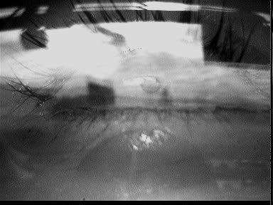
(a)

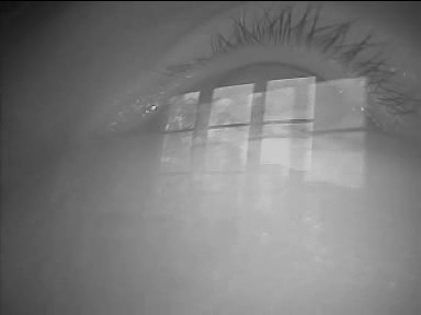
(b)

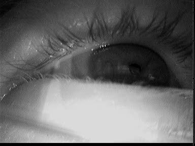
(c)

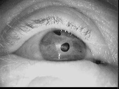
(d)

Figure 1: Images of typical pupil detection challenges in real-world scenarios: (a) and (b) reflections, (c) pupil located in dark area, and (d) unexpected physiological structures.

State-of-the-art pupil detection methods range from relatively simple methods such as combining thresholding and mass center estimation Peréz et al. [12] to more elaborated methods that attempt to identify the presence of reflections in the eye image and apply pupil-detection methods specifically tailored to handle such challenges Fuhl et al. [13] – a comprehensive review is given in Section 2. Despite substantial improvements over earlier methods in real-world scenarios, these current algorithms still present unsatisfactory detection rates in many important realistic use cases (as low as 34% Fuhl et al. [13]). However, in this work we show that carefully designed and trained convolutional neural networks (CNN) Domingos [14], LeCun et al. [15], which rely on statistical learning rather than hand-crafted heuristics, are a substantial step forward in the field of automated pupil detection. CNNs have been shown to reach human-level performance on a multitude of pattern recognition tasks (e.g., digit recognition Ciresan et al. [16], image classification Krizhevsky et al. [17]). These networks attempt to emulate the behavior of the visual processing system and were designed based on insights from visual perception research.

We propose a dual convolutional neural network pipeline for image-based pupil detection. The first pipeline stage employs a shallow CNN on subregions of a downscaled version of the input image to quickly infer a coarse estimate of the pupil location. This coarse estimation allows the second stage to consider only a small region of the original image, thus, mitigating the impact of noise and decreasing computational costs. The second pipeline stage then samples a small window around the coarse position estimate and refines the initial estimate by evaluating subregions derived from this window using a second CNN. We have focused on robust learning strategies (batch learning) instead of more accurate ones (stochastic gradient descent) LeCun et al. [18] due to the fact that an adaptive approach has to handle noise (e.g., illumination, occlusion, interference) effectively. The motivation behind the proposed pipeline is (i) to reduce the noise in the coarse estimation of the pupil position, (ii) to reliably detect the exact pupil position from the initial estimate, and (iii) to provide an efficient method that can be run in real-time on hardware architectures without an accessible GPU.

A further contribution of this work is a new hand-labeled data set with more than 40,000 eye images recorded in real world experiments. This data set consists of highly challenging eye images containing scattered reflections on glasses covering the parts or the complete pupil, pupils in dark areas whereby the contrast to the surrounding area is low, and additional black blobs on the iris, which may result from eye surgery. In addition, we propose a method for generating training data in an online-fashion, thus being applicable to the task of pupil center detection in online scenarios. We evaluated the performance of different CNN configurations both in terms of quality and efficiency and report considerable improvements over stat-of-the-art techniques.

2 Related work

During the last two decades, several algorithms have addressed image-based pupil detection. Peréz et al. [12] first thresholded the image and compute the mass center of the resulting dark pixels. This process was iteratively repeated in an area around the previously estimated mass center to determine a new mass center until convergence. The Starburst algorithm, proposed by Li et al. [19], first removed the corneal reflection and then located pupil edge points using an iterative feature-based approach. Based on the RANSAC algorithm Fischler and Bolles [20], a best fitting ellipse is determined, and the final ellipse parameters are selected by applying a model-based optimization. Long et al. [21] first down sampled the image and search there for an approximate pupil location. The image area around this location was further processed and a parallelogram-based symmetric mass center algorithm is applied to locate the pupil center. In another approach, Lin et al. [22] thresholded the image, removed artifacts by means of morphological operations, and applied inscribed parallelograms to determine the pupil center. Keil et al. [23] first located corneal reflections; afterwards, the input image was thresholded, the pupil blob was searched in the adjacency of the corneal reflection, and the centroid of pixels belonging to the blob was taken as pupil center. San Agustin et al. [24] threshold the input image and extract points in the contour between pupil and iris, which were then fitted to an ellipse based on the RANSAC method to eliminate possible outliers. Świrski et al. [25] started with a coarse positioning using Haar-like features. The intensity histogram of the coarse position was clustered using k-means clustering, followed by a modified RANSAC-based ellipse fit. The above approaches have shown good detection rates and robustness in controlled settings, i.e., laboratory conditions.

Three recent methods, SET Javadi et al. [26], ExCuSe Fuhl et al. [13], and ElSe Fuhl et al. [27], explicitly address the aforementioned challenges associated with pupil detection in natural environments. SET Javadi et al. [26] first extracts pupil pixels based on a luminance threshold. The resulting image is then segmented, and the segment borders are extracted using a Convex Hull method. Ellipses are fit to the segments based on their sinusoidal components, and the ellipse closest to a circle is selected as pupil. ExCuSe Fuhl et al. [13] first analyzes the input image with regard to reflections based on intensity histograms. Several processing steps based on edge detectors, morphologic operations, and the Angular Integral Projection Function are then applied to extract the pupil contour. Finally, an ellipse is fit to this line using the direct least squares method. ElSe Fuhl et al. [27] is based on the same edge based approach as ExCuSe Fuhl et al. [13] with further modifications like improved morphologic operations and line segment filtering by applying an ellipse fit. In addition the Angular Integral Projection function is replaced by a weighted blob detector. Although the latter three methods report substantial improvements over earlier methods, noise still remains a major issue. Thus, robust detection, which is critical in many online real-world applications, remains an open and challenging problem Fuhl et al. [28].

Recent developments in machine learning, especially in the field of neuronal networks, had a big breakthrough by learning cascaded filter banks, e.g., Krizhevsky et al. [17], LeCun et al. [15]. In particular for computer vision, there are three main advantages of CNNs when compared to fully connected neuronal networks. First, the convolution layers, which are linear filter banks learned by the CNN can be seen as neuronal network layers with shared weights.In image processing, this is achieved by convolving the weights with the input layer. As a result, these filters are shift-invariant and applicable to the entire image (since image statistics are stationary). Furthermore, only the local neighborhood of a location has an influence on the result, i.e, the spatial information of the response remains through to the neuron position. Each convolution layer has many of these filters and is usually followed by a pooling layer. The pooling layer subsamples the data and therefore reduces noise. The second advantage is the topological structure of a CNN, which arises from cascading multiple convolution layers. This allows to learn features from lower level features, which is generally known as deep learning. The third advantage is the consecutive reduction of the parameters in comparison to a fully connected neuronal network, which results from the topological structure.

Recent developments in CNNs are multi scale layers Gong et al. [29], Cai et al. [30], the inclusion of transposed convolutional layers (approximated deconvolution) Xu et al. [31], Long et al. [32] and recurrent CNNs Liang and Hu [33], Pinheiro and Collobert [34]. For example, the multi scale approach by Gong et al. [29] is based on spatial pyramid matching from Lazebnik et al. [35]. The input image is processed on multiple scales using ImageNet from Krizhevsky et al. [17]. The extracted feature vectors are than feed into a CNN. This approach was evaluated for classification, recognition, and image retrieval. Cai et al. [30] proposed a CNN architecture with fixed input size capable of handling multiple object sizes. This multi scale CNN follows the idea of training multiple detectors for each object size summarized in one CNN. For training they used a multi-task loss formulation where each label consists of the class and the enclosing bounding box. Another interesting development is the use of recurrent neuronal networks Carpenter and Grossberg [36] as convolution layer. The idea behind recurrent neuronal networks is the usage of information from previous computations. Liang and Hu [33] proposed the recurrent convolution layer based approach and showed its applicability for image recognition. For scene labeling Pinheiro and Collobert [34] proposed an architecture, which corrects itself due to this recurrence information. If it is about detection all mentioned architectures have to be applied to multiple image locations in a sliding window approach, due to the fact that each layer reduces the output size. CNNs with transposed convolutional layers address this problem by spreading the convolution of one location to multiple positions in the output. These layers approximate a deconvolution. The architecture with transposed convolutional layers was first proposed by Long et al. [32]. Alternatively Xu et al. [31] trained a CNN to learn real deconvolution filters for image restoration. The architecture of the net consists of large one dimensional kernels which represent the separable deconvolution filters.

In our scenario, we want to train a CNN for real time pupil center detection based on the CPU. Therefore most of the extensions like recurrent neuronal networks, deconvolution or multi scale networks remain prohibitively expensive. We used the classical window based approach with coarse and fine positioning to reduce the computational costs of convolutions. In addition, we propose a fast direct approach.

3 Proposed single- and two-stage CNN approaches

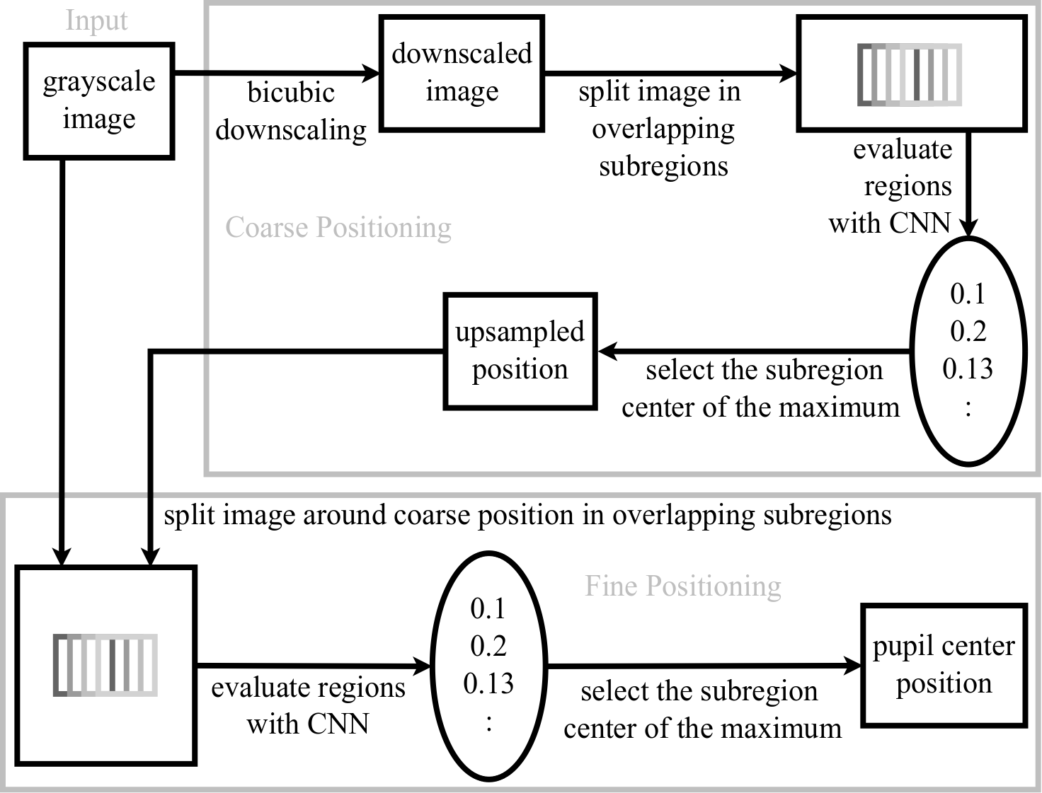
Figure 2: Workflow of the proposed algorithm. First a CNN is employed to estimate a coarse pupil position based on subregions from a downscaled version of the input image. This position is upsampled to the full resolution of the input image (upsampled position in the workflow diagram). This position is then refined using subregions around the coarse estimation in the original input image by a second CNN.

The overall workflow for the proposed algorithm is shown in Fig. 2. In the first stage, the image is downscaled and divided into overlapping subregions. These subregions are evaluated by the first CNN, and the center of the subregion that evokes the highest CNN response is used as a coarse pupil position estimate. Afterwards, this initial estimate is fed into the second pipeline stage. In this stage, subregions surrounding the initial estimate of the pupil position in the original input image are evaluated using a second CNN. The center of the subregion that evokes the highest CNN response is chosen as the final pupil center location. This two-step approach has the advantage that the first step (i.e., coarse positioning) has to handle less noise because of the bicubic downscaling of the image and, consequently, involves less computational costs than detecting the pupil on the complete upscaled image. In the following subsections, we delineate these pipeline stages and their CNN structures in detail, followed by the training procedure employed for each CNN.

3.1 Overview of all CNNs

Table 1: Overview of all evaluated CNN configurations. In row CNN the assigned names can be seen. C stands for convolution filter size, K is the amount of kernels (or filters), D stands for the pooling layer where D comes from down sampling and P stands for the amount of perceptron weights in the fully connected layer.

			Layer 1			Layer 2
		CNN	C	K	D	C	K	D	P
	Coarse	$CK_{8}P_{8}$	5	8	4	5	8	-	8
		$CK_{8}P_{16}$	5	8	4	5	16	-	16
		$CK_{16}P_{32}$	5	16	4	5	32	-	32
	Fine	$F_{CK_{X}P_{Y}}$	20	8	5	14	8	-	8
	Direct	$SK_{8}P_{8}$	6	8	4	5	8	-	8
	Fine	$F_{SK_{8}P_{8}}$	20	8	5	14	8	-	8

Table 1 shows an overview of all CNN configurations with their assigned names. All coarse CNNs follow the core architecture presented in Section 3.1.1, and each candidate has a specific number of filters in the convolution layer as well as perceptron weights in the fully connected layer. Their names ($CK_{X}P_{Y}$) are prefixed with C (Coarse) using X Kernels in the first layer and Y connections to the final Perceptron in the fully connected layer. The second stage CNN (see Figure 2) is named Fine CNN. The name ($F_{CK_{X}P_{Y}}$) specifies also the assigned coarse positioning CNN. This CNN is further described in Section 3.1.2. The last CNN is the direct pupil center estimation approach $SK_{8}P_{8}$, where only one Single stage is used based on the downsampled image. Those are described in Section 3.2.3. However, we evaluated $SK_{8}P_{8}$ also with the two step approach ($F_{SK_{8}P_{8}}$).

3.1.1 Coarse positioning CNN ($CK_{8}P_{8}$, $CK_{8}P_{16}$, $CK_{16}P_{32}$)

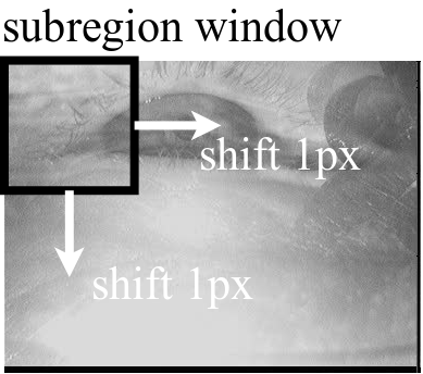
(a)

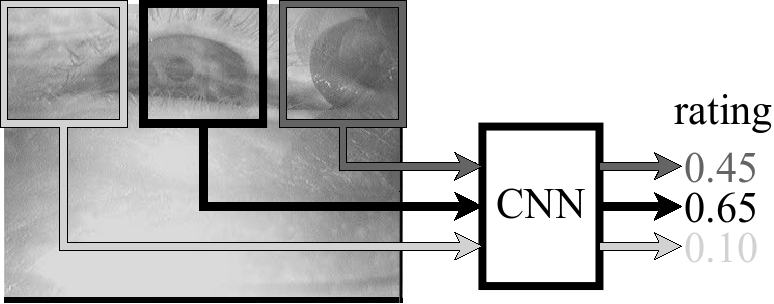
(b)

Figure 3: The downscaled image is divided in subregions of size $24\times 24$ pixels with a stride of one pixel (a), which are then rated by the first stage CNN (b).

The grayscale input images generated by the mobile eye tracker used in this work are sized $384\times 288$ pixels. Directly employing CNNs on images of this size would demand a large amount of resources and, thus, would be computationally expensive, impeding their usage in state-of-the-art mobile eye trackers. Thus, one of the purposes of the first stage is to reduce computational costs by providing a coarse estimate that can in turn be used to reduce the search space of the exact pupil location. However, the main reason for this step is to reduce noise, which can be induced by different camera distances, changing sensory systems between head-mounted eye trackers Boie and Cox [37], Dussault and Hoess [38], Reibel et al. [39], movement of the camera itself, or the usage of uncalibrated cameras (e.g., out of focus, unbalanced white levels). To achieve this goal, first the input image is downscaled using a bicubic interpolation, which employs a third order polynomial in a two dimensional space to evaluate the resulting values. In our implementation, we employ a downscaling factor of four times, resulting in images of $96\times 72$ pixels. Given that these images contain the entire eye, we chose a CNN input size of $24\times 24$ pixels to guarantee that the pupil is fully contained within a subregion of the downscaled images. Subregions of the downscaled image are extracted by shifting a $24\times 24$ pixels window with a stride of one pixel (see Fig. 3a) and evaluated by the CNN, resulting in a rating within the interval [0,1] (see Fig. 3b).

These ratings represent the confidence of the CNN that the pupil center is within the subregion. Thus, the center of the highest rated subregion is chosen as the coarse pupil location estimation. The core architecture of the first stage CNN is summarized in Table 1. The first layer is a convolutional layer with filter size $5\times 5$ pixels, one pixel stride, and no padding. The convolution layer is followed by an average pooling layer with window size $4\times 4$ pixels and four pixels stride. The subsequent stage is an additional convolution layer with filter size $5\times 5$, reducing the size of the feature map to $1\times 1\times 8$, which is fed into the last fully connected layer with depth one. The last layer can be seen as a single perceptron responsible for yielding the final rating within the interval [0,1]. The size of the filter in combination with the pooling size is a trade-off between the information the CNN can hold and its computational costs. Many small convolution layers would increase the processing time of the net; in contrast, higher pooling would reduce the information held by the CNN.

We have evaluated this architecture for different amounts of filters in the convolutional layers as well as varying the quantity of perceptrons in the fully connected layer; these values are reported in Section 5. The main idea behind the selected architecture is that the convolutional layer learns basic features, such as edges, approximating the pupil structure. The average pooling layer makes the CNN robust to small translations and blurring of these features (e.g., due to the initial downscaling of the input image). The second convolution layer incorporates deeper knowledge on how to combine the learned features for the coarse detection of the pupil position. The final perceptron learns a weighting to produce the final rating.

3.1.2 Fine positioning CNN ($F_{CK_{X}P_{Y}}$and $F_{SK_{8}P_{8}}$)

Although the first stage yields an accurate pupil position estimate, it lacks precision due to the inherent error introduced by the downscaling step. Therefore, it is necessary to refine this estimate. This refinement could be attempted by applying methods similar to those described in Section 2 to a small window around the coarse pupil position estimate. However, since most of the previously mentioned challenges are not alleviated by using this small window, we chose to use a second CNN that evaluates subregions surrounding the coarse estimate in the original image.

The second stage CNN employs the same architecture pattern as the first stage (i.e., convolution $\Rightarrow$ average pooling $\Rightarrow$ convolution $\Rightarrow$ fully connected) since their motivations are analogous. Nevertheless, this CNN operates on a larger input resolution to increase accuracy and precision. Intuitively, the input image for this CNN would be $96\times 96$ pixels: the input size of the first CNN input ($24\times 24$) multiplied by the downscaling factor ($4$). However, the resulting memory requirement for this size was larger than available on our test device; as a result, we utilized the closest working size possible: $89\times 89$ pixels. The size of the other layers were adapted accordingly. The convolution filters in the first layer were enlarged to $20$ pixels to compensate for increased noise and motion blur. The dimension of the pooling window was increased by one pixel, leading to a decreased input size on the second convolution layer and reduced runtime.

This CNN uses eight convolution filters in the first stage and eight perceptron weights due to the increased size of the convolution filter and the input region size. Subregions surrounding the coarse pupil position are extracted based on a window of size $89\times 89$ pixels centered around the coarse estimate, which is shifted in a radius of $10$ pixels (with a one pixel stride) horizontally and vertically. Analogously to the first stage, the center of the region with the highest CNN rating is selected as fine pupil position estimate. Despite higher computational costs in the second stage, our approach is highly efficient and can be run on today’s conventional mobile eye-tracking systems.

3.1.3 Direct coarse to fine positioning CNN ($SK_{8}P_{8}$)

Unfortunately, the fine positioning CNN requires computational capabilities that are not always found in state-of-the-art embedded systems. To address this issue, we have developed one additional fine positioning method for this evaluation that employs a CNN similar to the ones used in the coarse positioning stage. However, this CNN uses an input size of $25\times 25$ pixels to obtain an even center. As a consequence, the first convolution layer was increased to $6\times 6$ filters. This method is used as an inexpensive single stage approach ($SK_{8}P_{8}$) as well as in combination with the fine positioning CNN ($F_{SK_{8}P_{8}}$).

3.2 CNN training methodology

Both CNNs were trained using supervised batch gradient descent LeCun et al. [18] with a dynamic learning rate from $10^{-1}$ to $10^{-6}$. The learning rate was dropped after each ten epochs by $10^{-1}$. In the first round we trained for $50$ epochs and selected the best performing CNN on the validation set. This was repeated four times and in each new round the starting learning rate was decreased by a factor of $10^{-1}$. After the last round we did fine tuning by inspecting each iteration additionally. For each round we generated a new training set. The batch size for one iteration was $100$ and all CNNs’ weights were initialized using a Gaussian with standard deviation of $0.01$. While stochastic gradient descent searches for minima in the error plane more effectively than batch learning when given valid examples Heskes and Kappen [40], Orr [41], it is vulnerable to disastrous hops if given inadequate examples (e.g., due to poor performance of the traditional algorithm). On the contrary, batch training dilutes this error which is why we have opted for this method.

3.2.1 Coarse positioning CNN ($CK_{8}P_{8}$, $CK_{8}P_{16}$, $CK_{16}P_{32}$)

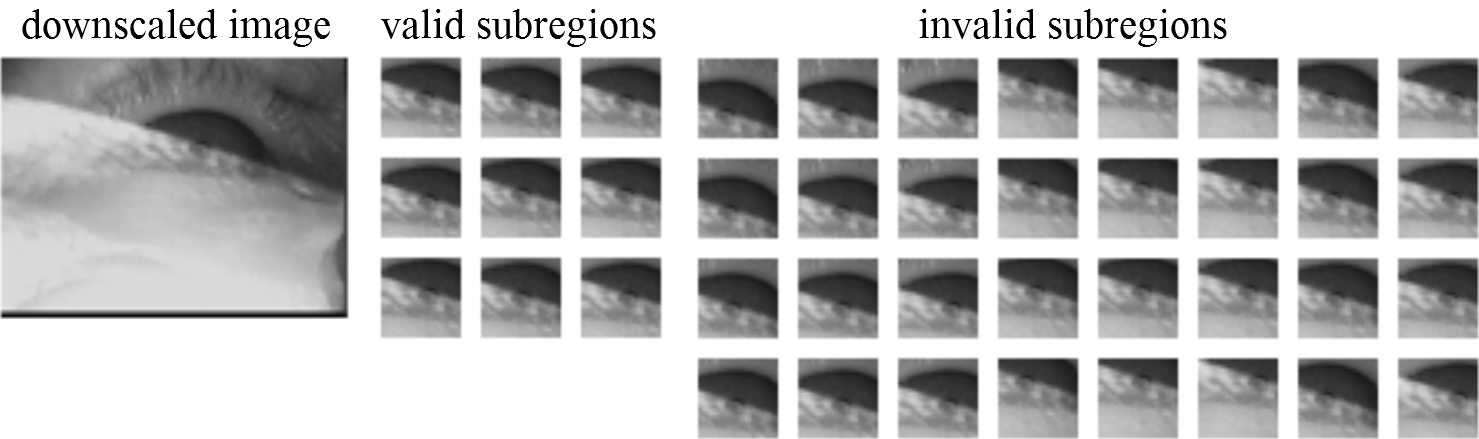
Figure 4: Nine valid (top right) and 32 invalid (bottom) training samples for the coarse position CNN extracted from a downscaled input image (top left).

The coarse position CNN was trained on subregions extracted from the downscaled input images that fall into two different data classes: containing a valid ($label=1$) or invalid ($label=0$) pupil center. Training subregions were extracted by collecting all subregions with center distant up to twelve pixels from the hand-labeled pupil center. In the first round of training we only used half of the distance to reduce the amount of invalid examples. Subregions with center distant up to one pixel were labeled as valid examples while the remaining subregions were labeled as invalid examples. As exemplified by Fig. 4, this procedure results in an unbalanced set of valid and invalid examples therefore we only used samples on the diagonal (top left to bottom right) where every second was discarded for the invalid samples. This reduces the amount of samples per frame. Due to the huge size difference of the data sets we reduced the amount of samples per set to 20,000 for the first round and 40,000 for the others. Therefore we picked randomly two thousand images per data set, created the samples and dropped the overflow. If the data set was to small we copied the samples to reach the 20,000 or 40,000.

3.2.2 Fine positioning CNN ($F_{CK_{X}P_{Y}}$and $F_{SK_{8}P_{8}}$)

The fine positioning CNN (responsible for detecting the exact pupil position) is trained similarly to the coarse positioning one. However, we extract only valid subregion up to a distance of three pixels from the hand-labeled pupil center and selected samples up to a distance of twenty four pixels with a step size of three. Afterwards the valid examples where again copied to balance the amount of valid and invalid examples. This reduced amount of samples per hand-labeled data ad is to constrain learning time, as well as main memory and storage consumption.

3.2.3 Direct coarse to fine positioning CNN ($SK_{8}P_{8}$)

For these CNNs, training and evaluation were performed in an analogous fashion to the previous ones, with the exception that training samples were generated from both diagonals (top left to bottom right and top right to bottom left).

3.3 Fast fine accuracy improvement

The main idea here is to use the response of the CNN surrounding the maximum value to refine the pupil center estimation.

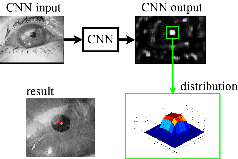
Figure 5: The work flow of the accuracy improvement. On the top left the input image is shown, on the top right is the output of the CNN. For accuracy improvement the surrounding area of the maximum position is converted to a distribution and a shift vector is computed. This distribution is shown in the green box on the bottom right. On the bottom left the maximum position (red dot) and the shifted position (green dot) are shown.

For a fast accuracy improvement of all CNNs the response surrounding the maximum position is converted into a probability distribution. Such a response of a CNN is shown in figure 5 on the top left. The converted area is surrounded by a green square. In our implementation we used an $7\times 7$ ($N\times M$) square centered at the maximum position. The resulting distribution is shown in Figure 5 on the bottom right. To convert the response into a distribution each value is divided by the sum of all values in the square (equation (1)).

$$D(x,y)=\frac{R(x,y)}{\sum_{i=0}^{N}\sum_{j=0}^{M}R(i,j)}$$ (1)

In equation (1) $D(x,y)$ is the distribution value at location $x,y$ and $R(x,y)$ is the CNN response at location $x,y$. Each value in this distribution is weighted by the displacement vector to the maximum position. The calculation is shown in equation (2).

$$\overrightarrow{SV}=\sum_{i=-\frac{N}{2}}^{\frac{N}{2}}\sum_{j=-\frac{M}{2}}^{\frac{M}{2}}D(\frac{N}{2}+i,\frac{M}{2}+j)*\left(\hskip-5.0pt\begin{array}[]{r}i\@arraycr j\end{array}\hskip-5.0pt\right)$$ (2)

In equation (2) $\overrightarrow{SV}$ is the vector shifting the initial maximum position (red dot in figure 5 on the bottom left) to the new more accurate position (green dot in figure 5 on the bottom left). $D(i,j)$ is the result of equation (1) at location $i,j$ and $\left(\hskip-5.0pt\begin{array}[]{r}i\@arraycr j\end{array}\hskip-5.0pt\right)$ is the displacement vector to the center.

4 Data sets

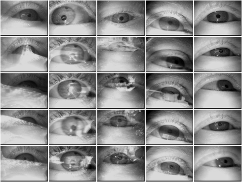
Figure 6: Samples from the data sets contributed by this work. Each column belongs to a distinct data set. The top row includes non-challenging samples, which can be considered relatively similar to laboratory conditions and represent only a small fraction of each data set. The other two rows include challenging samples with artifacts caused by the natural environment.

In this study, we used the data sets provided by Fuhl et al. [13, 27], complemented by five additional new hand-labeled data sets contributed by this work. In total, over 135,000 manually labeled eye images were employed for evaluation. Our data sets introduced with this work include 41,217 images collected during driving sessions in public roads for an experiment Kasneci [3] that were not related to pupil detection and were chosen due the non-satisfactory performance of the proprietary pupil detection algorithm. These new data sets include fast changing and adverse illumination, spectacle reflections, and disruptive physiological eye characteristics (e.g., dark spot on the iris); samples from these data sets are shown in Fig. 6.

5 Evaluation

Training and evaluation figures reported in this paper were obtained on an Intel^® Core™i5-4670 desktop computer with 8GB RAM. This setup was chosen because it provides a performance similar to systems that are usually provided by eye-tracker vendors, thus enabling the actual eye-tracking system to perform other experiments along with the evaluation. The algorithm was implemented using MATLAB (r2015b) combined with caffe Jia et al. [42]. We report our results in terms of the average pupil detection rate as a function of pixel distance between the algorithmically established and the hand-labeled pupil center. Although the ground truth was labeled by experts in eye-tracking research, imprecision cannot be excluded. Therefore, the results are discussed for a pixel error of five (i.e., pixel distance between the algorithmically established and the hand-labeled pupil center), analogously to Fuhl et al. [13], Świrski et al. [25].
We performed a per data set cross validation guaranteeing that the CNNs are evaluated on distinct images from those it was trained on. In addition this gives us the advantage for a more detailed comparison between PupilNet and the state-of-the-art algorithms.

5.1 Coarse positioning

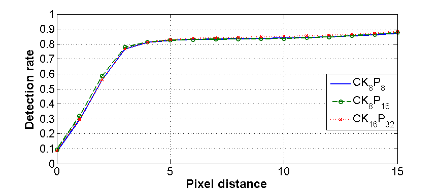
Figure 7: Performance for the evaluated coarse CNNs using the per data set cross validation showing the downscaled error ($*4$ for real error). Each data set is weighted equally meaning that the average result over all data sets is shown independent of their image count.

We start by evaluating the candidates from Table 1 for the coarse positioning CNN. Fig. 7 shows the performance of the coarse positioning CNNs when trained using the per data set cross validation. As can be seen in figure 7, the number of filters in the first layer ($CK_{8}P_{8}$, and $CK_{8}P_{16}$) have only a small impact to the detection rate. Increasing the amount for both convolutions ($CK_{16}P_{32}$) improves the result slightly but also increases the computational costs (Fig. 7 shows he average detection rate over all data sets meaning that one percent improvement means an betterment on all data sets). However, it is important to notice that this is the most expensive parameter in the proposed CNN architecture in terms of computation time and, thus, further increments must be carefully included.

5.2 Fine positioning

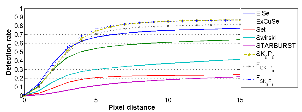
Figure 8: All CNNs were trained and evaluated using the per data set cross validation. The average detection rate over all data sets is shown. The result for $SK_{8}P_{8}$ is with accuracy improvement from section 3.3.

Table 2: Five pixel error for the proposed CNNs and the state-of-the-art per data set.

	ElSe	ExCuSe	$SK_{8}P_{8}$	$F_{CK_{X}P_{Y}}$	$F_{SK_{X}P_{Y}}$
I	0.86	0.72	0.77	0.78	0.82
II	0.65	0.40	0.80	0.79	0.79
III	0.64	0.38	0.62	0.60	0.66
IV	0.83	0.80	0.90	0.90	0.92
V	0.85	0.76	0.91	0.89	0.92
VI	0.78	0.60	0.73	0.78	0.79
VII	0.60	0.49	0.73	0.80	0.73
VIII	0.68	0.55	0.84	0.83	0.81
IX	0.87	0.76	0.86	0.86	0.86
X	0.79	0.79	0.80	0.78	0.81
XI	0.75	0.58	0.85	0.74	0.91
XII	0.79	0.80	0.87	0.85	0.85
XIII	0.74	0.69	0.79	0.81	0.83
XIV	0.84	0.68	0.91	0.94	0.95
XV	0.57	0.56	0.81	0.71	0.81
XVI	0.60	0.35	0.80	0.72	0.80
XVII	0.90	0.79	0.99	0.87	0.97
XVIII	0.57	0.24	0.55	0.44	0.62
XIX	0.33	0.23	0.34	0.20	0.37
XX	0.78	0.58	0.79	0.73	0.79
XXI	0.47	0.52	0.81	0.67	0.83
XXII	0.53	0.26	0.50	0.52	0.58
XXIII	0.94	0.93	0.86	0.87	0.90
XXIV	0.53	0.46	0.46	0.55	0.55
new I	0.62	0.22	0.69	0.56	0.69
new II	0.26	0.16	0.44	0.35	0.45
new III	0.39	0.34	0.45	0.44	0.49
new IV	0.54	0.48	0.83	0.77	0.82
new V	0.75	0.59	0.78	0.76	0.81

The $F_{CK_{X}P_{Y}}$was evaluated using all the previously evaluated coarse CNNs (i.e., $CK_{8}P_{8}$, $CK_{8}P_{16}$, and $CK_{16}P_{32}$). In addition the direct approach $SK_{8}P_{8}$ was evaluated with the accuracy correction from Section 3.3. Similarly to the coarse positioning, these were also evaluated through the per data set cross validation.

As baseline, we evaluated five state-of-the-art algorithms, namely, ElSe Fuhl et al. [27], ExCuSe Fuhl et al. [13], SET Javadi et al. [26], Starburst Li et al. [19], and Świrski et al. [25]. The average performance of the evaluated approaches is shown in Fig. 8.

As can be seen in the figure, all two-stage CNNs surpass the best performing state-of-the-art approach ElSe Fuhl et al. [27] by $\approx 4$% and $\approx 9$%. Although the proposed two stage approaches ($F_{CK_{X}P_{Y}}$and $F_{SK_{8}P_{8}}$) reach the best pupil detection rate in average per data set at a pixel error of five, it is worth highlighting the performance of the $SK_{8}P_{8}$ ($\approx 7$% over the state-of-the-art) with its reduced computational costs (runtime of 7ms on a intel i5-4570 3.2GHz single core). This low runtime was reached by only evaluating every second image position in the first step and afterwards extracting the CNN responses on a per pixel level only surrounding the found maximum. The final optimization applied to this region is described in section 3.3. In comparison ElSe has a runtime of 7ms, ExCuSe 6ms and Świrski et al. [25] 8ms. Starburst and SET are not comparable because we used the MATLAB implementation. $F_{CK_{X}P_{Y}}$has a runtime of 1.2 seconds where in the first step $CK_{8}P_{8}$ is used with a runtime of 6ms. Due to the lower accuracy of $CK_{8}P_{8}$ in comparison to $SK_{8}P_{8}$ we had to increase the search region of $F_{CK_{X}P_{Y}}$($49\times 49$). This large search region and the high computational costs of $F_{CK_{X}P_{Y}}$forced us to only evaluate every second image position. For $F_{SK_{8}P_{8}}$ we used $SK_{8}P_{8}$ as coarse positioning CNN followed by a fine positioning in a $21\times 21$ search region. $F_{SK_{8}P_{8}}$ has a runtime of 850ms. Due to the architecture of CNNs both approaches $F_{CK_{X}P_{Y}}$and $F_{SK_{8}P_{8}}$ are fully parallelizable with a runtime per patch ($89\times 89$) of 2ms. For a finer comparison at a pixel error of five, all results are shown in Table 2.

6 Conclusion

We presented a naturally motivated pipeline of specifically configured CNNs for robust pupil detection and showed that it outperforms state-of-the-art approaches while avoiding high computational costs. For the evaluation we used over 135,000 hand labeled images – 41,000 of which were contributed by this work – from real-world recordings with artifacts such as reflections, changing illumination conditions, and occlusions. Specially for these challenging data sets, the CNNs reported considerably higher detection rates than state-of-the-art techniques. Looking forward, we are planning to investigate the applicability of the proposed pipeline to online scenarios, where continuous adaptation of the parameters is a further challenge. For further research and usage, data sets, source code for data generation and training, as well as the trained CNNs will be made available for download.

References

- Wade and Tatler [2005] N. Wade, B. W. Tatler, The moving tablet of the eye: The origins of modern eye movement research, Oxford University Press, 2005.
- Yarbus [1957] A. Yarbus, The perception of an image fixed with respect to the retina, Biophysics 2 (1) (1957) 683–90.
- Kasneci [2013] E. Kasneci, Towards the automated recognition of assistance need for drivers with impaired visual field, Ph.D. thesis, Universität Tübingen, Germany, 2013.
- Turner et al. [2013] J. Turner, J. Alexander, A. Bulling, D. Schmidt, H. Gellersen, Eye pull, eye push: Moving objects between large screens and personal devices with gaze and touch, in: Human-Computer Interaction–INTERACT 2013, Springer, 170–86, 2013.
- Cowen et al. [2002] L. Cowen, L. J. Ball, J. Delin, An eye movement analysis of web page usability, in: People and Computers XVI-Memorable Yet Invisible, Springer, 317–35, 2002.
- Kassner et al. [2014] M. Kassner, W. Patera, A. Bulling, Pupil: an open source platform for pervasive eye tracking and mobile gaze-based interaction, in: Proceedings of the 2014 ACM International Joint Conference on Pervasive and Ubiquitous Computing: Adjunct Publication, ACM, 1151–60, 2014.
- Liu et al. [2002] X. Liu, F. Xu, K. Fujimura, Real-time eye detection and tracking for driver observation under various light conditions, in: Intelligent Vehicle Symposium, 2002. IEEE, vol. 2, 2002.
- Trösterer et al. [2014] S. Trösterer, A. Meschtscherjakov, D. Wilfinger, M. Tscheligi, Eye Tracking in the Car: Challenges in a Dual-Task Scenario on a Test Track, in: Proceedings of the 6th AutomotiveUI, ACM, 2014.
- Kasneci et al. [2014] E. Kasneci, K. Sippel, M. Heister, K. Aehling, W. Rosenstiel, U. Schiefer, E. Papageorgiou, Homonymous Visual Field Loss and Its Impact on Visual Exploration: A Supermarket Study, TVST 3.
- Schnipke and Todd [2000] S. K. Schnipke, M. W. Todd, Trials and tribulations of using an eye-tracking system, in: CHI’00 ext. abstr., ACM, 2000.
- Santini et al. [2016] T. Santini, W. Fuhl, T. C. Kübler, E. Kasneci, Bayesian identification of fixations, saccades, and smooth pursuits, in: Proceedings of the Ninth Biennial ACM Symposium on Eye Tracking Research & Applications, ETRA 2016, Charleston, SC, USA, March 14-17, 2016, 163–70, doi:, URL http://doi.acm.org/10.1145/2857491.2857512, 2016.
- Peréz et al. [2003] A. Peréz, M. Cordoba, A. Garcia, R. Méndez, M. Munoz, J. L. Pedraza, F. Sanchez, A precise eye-gaze detection and tracking system .
- Fuhl et al. [2015a] W. Fuhl, T. Kübler, K. Sippel, W. Rosenstiel, E. Kasneci, ExCuSe: Robust Pupil Detection in Real-World Scenarios, in: CAIP 16th Inter. Conf., Springer, 2015a.
- Domingos [2012] P. Domingos, A few useful things to know about machine learning, Communications of the ACM 55 (10) (2012) 78–87.
- LeCun et al. [1998] Y. LeCun, L. Bottou, Y. Bengio, P. Haffner, Gradient-based learning applied to document recognition, Proceedings of the IEEE 86 (11) (1998) 2278–324.
- Ciresan et al. [2012] D. Ciresan, U. Meier, J. Schmidhuber, Multi-column deep neural networks for image classification, in: Computer Vision and Pattern Recognition (CVPR), 2012 IEEE Conference on, IEEE, 3642–9, 2012.
- Krizhevsky et al. [2012] A. Krizhevsky, I. Sutskever, G. E. Hinton, Imagenet classification with deep convolutional neural networks, in: Advances in neural information processing systems, 1097–105, 2012.
- LeCun et al. [2012] Y. A. LeCun, L. Bottou, G. B. Orr, K.-R. Müller, Efficient backprop, in: Neural networks: Tricks of the trade, Springer, 9–48, 2012.
- Li et al. [2005] D. Li, D. Winfield, D. J. Parkhurst, Starburst: A hybrid algorithm for video-based eye tracking combining feature-based and model-based approaches, in: CVPR Workshops 2005. IEEE Computer Society Conference on, IEEE, 2005.
- Fischler and Bolles [1981] M. A. Fischler, R. C. Bolles, Random sample consensus: a paradigm for model fitting with applications to image analysis and automated cartography, Communications of the ACM 24 (6) (1981) 381–95.
- Long et al. [2007] X. Long, O. K. Tonguz, A. Kiderman, A high speed eye tracking system with robust pupil center estimation algorithm, in: EMBS 2007, IEEE, 2007.
- Lin et al. [2010] L. Lin, L. Pan, L. Wei, L. Yu, A robust and accurate detection of pupil images, in: BMEI 2010, vol. 1, IEEE, 2010.
- Keil et al. [2010] A. Keil, G. Albuquerque, K. Berger, M. A. Magnor, Real-Time Gaze Tracking with a Consumer-Grade Video Camera .
- San Agustin et al. [2010] J. San Agustin, H. Skovsgaard, E. Mollenbach, M. Barret, M. Tall, D. W. Hansen, J. P. Hansen, Evaluation of a low-cost open-source gaze tracker, in: Proceedings of the 2010 Symposium on Eye-Tracking Research & Applications, ACM, 77–80, 2010.
- Świrski et al. [2012] L. Świrski, A. Bulling, N. Dodgson, Robust real-time pupil tracking in highly off-axis images, in: Proceedings of the Symposium on ETRA, ACM, 2012.
- Javadi et al. [2015] A.-H. Javadi, Z. Hakimi, M. Barati, V. Walsh, L. Tcheang, SET: a pupil detection method using sinusoidal approximation, Frontiers in neuroengineering 8.
- Fuhl et al. [2015b] W. Fuhl, T. C. Santini, T. Kuebler, E. Kasneci, Else: Ellipse selection for robust pupil detection in real-world environments, arXiv preprint arXiv:1511.06575 .
- Fuhl et al. [2017] W. Fuhl, D. Hospach, T. Kuebler, W. Rosenstiel, O. Bringmann, E. Kasneci, Ways of improving the precision of eye tracking data: Controlling the influence of dirt and dust on pupil detection, Journal of Eye Movement Research 10 (3), ISSN 1995-8692, URL https://bop.unibe.ch/index.php/JEMR/article/view/3657.
- Gong et al. [2014] Y. Gong, L. Wang, R. Guo, S. Lazebnik, Multi-scale orderless pooling of deep convolutional activation features, in: European conference on computer vision, Springer, 392–407, 2014.
- Cai et al. [2016] Z. Cai, Q. Fan, R. S. Feris, N. Vasconcelos, A unified multi-scale deep convolutional neural network for fast object detection, in: European Conference on Computer Vision, Springer, 354–70, 2016.
- Xu et al. [2014] L. Xu, J. S. Ren, C. Liu, J. Jia, Deep convolutional neural network for image deconvolution, in: Advances in Neural Information Processing Systems, 1790–8, 2014.
- Long et al. [2015] J. Long, E. Shelhamer, T. Darrell, Fully convolutional networks for semantic segmentation, in: Proceedings of the IEEE Conference on Computer Vision and Pattern Recognition, 3431–40, 2015.
- Liang and Hu [2015] M. Liang, X. Hu, Recurrent convolutional neural network for object recognition, in: Proceedings of the IEEE Conference on Computer Vision and Pattern Recognition, 3367–75, 2015.
- Pinheiro and Collobert [2014] P. Pinheiro, R. Collobert, Recurrent convolutional neural networks for scene labeling, in: International Conference on Machine Learning, 82–90, 2014.
- Lazebnik et al. [2006] S. Lazebnik, C. Schmid, J. Ponce, Beyond bags of features: Spatial pyramid matching for recognizing natural scene categories, in: Computer vision and pattern recognition, 2006 IEEE computer society conference on, vol. 2, IEEE, 2169–78, 2006.
- Carpenter and Grossberg [1987] G. A. Carpenter, S. Grossberg, A massively parallel architecture for a self-organizing neural pattern recognition machine, Computer vision, graphics, and image processing 37 (1) (1987) 54–115.
- Boie and Cox [1992] R. A. Boie, I. J. Cox, An analysis of camera noise, IEEE Transactions on Pattern Analysis & Machine Intelligence .
- Dussault and Hoess [2004] D. Dussault, P. Hoess, Noise performance comparison of ICCD with CCD and EMCCD cameras, in: Optical Science and Technology, the SPIE 49th Annual Meeting, International Society for Optics and Photonics, 195–204, 2004.
- Reibel et al. [2003] Y. Reibel, M. Jung, M. Bouhifd, B. Cunin, C. Draman, CCD or CMOS camera noise characterisation, The European Physical Journal Applied Physics 21 (01) (2003) 75–80.
- Heskes and Kappen [1993] T. M. Heskes, B. Kappen, On-line learning processes in artificial neural networks, North-Holland Mathematical Library 51 (1993) 199–233.
- Orr [1995] G. B. Orr, Dynamics and algorithms for stochastic learning, Ph.D. thesis, PhD thesis, Department of Computer Science and Engineering, Oregon Graduate Institute, Beaverton, OR 97006, 1995. ftp://neural. cse. ogi. edu/pub/neural/papers/orrPhDch1-5. ps. Z, orrPhDch6-9. ps. Z, 1995.
- Jia et al. [2014] Y. Jia, E. Shelhamer, J. Donahue, S. Karayev, J. Long, R. Girshick, S. Guadarrama, T. Darrell, Caffe: Convolutional Architecture for Fast Feature Embedding, arXiv preprint arXiv:1408.5093 .