Constraining scalar resonances with top-quark pair production at the LHC

Abstract

Constraints on models which predict resonant top-quark pair production at the LHC are provided via a reinterpretation of the Standard Model (SM) particle level measurement of the top-anti-top invariant mass distribution, $m(t\bar{t})$. We make use of state-of-the-art Monte Carlo event simulation to perform a direct comparison with measurements of $m(t\bar{t})$ in the semi-leptonic channels, considering both the boosted and the resolved regime of the hadronic top decays. A simplified model to describe various scalar resonances decaying into top-quarks is considered, including CP-even and CP-odd, color-singlet and color-octet states, and the excluded regions in the respective parameter spaces are provided.

I Introduction

With its mass being close to the electroweak scale the top quark is very special. It might intimately be connected to the underlying mechanism of electroweak symmetry breaking (EWSB). Consequently, studying top-quark production and decays at colliders might provide a portal to New Physics (NP). The Large Hadron Collider (LHC), providing proton–proton collisions currently at 13 TeV centre-of-mass energy, can be seen as a top-quark factory. It allows to search for anomalous top-quark production and decay processes, considered as low energy modifications of the Standard Model (SM) parametrized by effective operators Barger:2011pu ; Choi:2012fc ; Franzosi:2015osa ; Zhang:2016omx ; Englert:2016aei ; Cirigliano:2016nyn , or, as the direct production of intermediate resonances, which have been hunted for a long time at different experiments Aaltonen:2009tx ; Khachatryan:2015sma ; Chatrchyan:2013lca .

Heavy scalar resonances that decay into a pair of top quarks are predicted by several NP scenarios, in particular the Two Higgs Doublet Model (THDM), supersymmetric theories and models of dynamical EWSB. In this paper, we provide a framework to reinterpret the SM $t\bar{t}$ differential cross section measurements as exclusion limits for signatures of NP resonances decaying into $t\bar{t}$. The framework relies on the comparison between particle-level data with state-of-the-art event simulation and the interpretation of deviations in terms of NP models. It is based on four main ingredients

1. A Monte Carlo event generator which allows the precise and realistic description of particle-level observables.

   In order to theoretically describe top-quark pair production at the LHC, we make use of state-of-the-art event simulations provided by the Sherpa Gleisberg:2008ta event-generator framework. This implies the usage of techniques to match leading and next-to-leading order QCD matrix elements with parton showers and merging different parton-multiplicity final states.

2. The precise measurement of SM processes from fiducial kinematical regions provided as differential particle-level observables by LHC experiments, and available through the Rivet package Buckley:2010ar . Here we used the ATLAS analyses of top-quark pair production in the boosted Aad:2015hna and resolved Aad:2015mbv regimes.

3. A general parametrization of NP whose predictions for colliders can be computed efficiently. We adopt a Lagrangian which describes scalar resonances that can be CP-even or odd and color singlet or octet. We devise a reweighting method to describe the model prediction in the $m(t\bar{t})$ distribution for a wide range of the parameter space in a fast and efficient manner.

4. A statistical interpretation to decide what regions of parameter space of the model are ruled out at a given confidence level. We adopt here a simplified $\chi^{2}$ analysis.

A similar method to constrain NP with SM measurements in several other channels has recently been presented in Ref. Butterworth:2016sqg . These approaches are complementary to model-specific searches in the respective final states. They provide systematic methods for the theory community to derive more realistic exclusion limits for any particular model, not relying on the experiment-specific assumptions.

In the rest of the paper we explain these 4 points in detail. In Sec. II we describe the set-up of our event simulation. In Sec. III we give details on the analyses used in the boosted and the resolved regime and validate our SM predictions by comparing them to experimental data. In Sec. IV we introduce our simplified model of beyond the SM scalar resonances and describe the implementation in our simulation framework, based on an event-by-event reweighting. In Sec. V we present a statistical analysis to assess the region in parameter space accessible by the LHC experiments and provide interpretations in terms of some specific models. We finally conclude in Sec. VI.

II Simulation framework

When searching for imprints of resonant contributions in top-quark pair production at the LHC, a detailed understanding of the SM production process is vital. In particular, as there are non-trivial interference effects between NP signals and SM amplitudes that determine the shape of the resulting top-pair invariant-mass distribution. In order to obtain realistic and reliable predictions for the top-pair production process, we make use of state-of-the-art particle-level simulations, based on higher-order matrix elements matched to parton-shower simulations and hadronization.

Our analysis focuses on observables in the semi-leptonic decay channel of top-quark pair production, i.e.

$$pp\to t\bar{t}\to b\bar{b}jj\ell\nu\text{ + jets}\,,$$ (1)

where $\ell$ denotes muons or electrons, $\nu$ the corresponding neutrinos, $b$ are bottom quarks and $j$ light quarks or gluons. These decay products and the associated radiation might be reconstructed as well-separated objects, i.e. light-flavour jets, $b$-jets and a lepton, or, in the boosted regime, as a large-area jet, containing the hadronic decay products, additional jets and a lepton. In either case, to realistically simulate the associated QCD activity, higher-order QCD corrections need to be considered.

To describe the SM top-pair production process we use the Sherpa event-generation framework Gleisberg:2003xi ; Gleisberg:2008ta . We employ the techniques to match LO and NLO QCD matrix elements to Sherpa’s dipole shower Schumann:2007mg and to merge processes of variable partonic multiplicity Hoeche:2009rj ; Hoeche:2012yf . Leading-order and real-emission correction matrix elements are obtained from Comix Gleisberg:2008fv . Virtual one-loop amplitudes, contributing at NLO QCD, are obtained from the Recola generator Actis:2016mpe ; Biedermann:2017yoi that employs the Collier library Denner:2016kdg . Top-quark decays are modelled at leading-order accuracy through Sherpa’s decay handler, that implements Breit-Wigner smearing for the intermediate resonances and preserves spin correlations between production and decay Hoche:2014kca . We treat bottom-quarks as massive in the top-quark decays and the final-state parton-shower evolution Krauss:2016orf .

To validate the SM predictions we also consider leading-order simulations in the MadGraph_aMCNLO framework Alwall:2014hca . The hard-process’ partonic configurations get showered and hadronized through Pythia8 Sjostrand:2014zea . The spin-correlated decays of top quarks are implemented through the MadSpin package Artoisenet:2012st . Samples of different partonic multiplicity are merged according to the $k_{T}$-MLM prescription described in Alwall:2007fs .

For the top-quark and $W$-boson, the following mass values are used

$$m_{t}=172\;{\rm GeV}\,,\quad m_{W}=80.39\;{\rm GeV}\,,$$ (2)

and the corresponding widths are calculated at leading order, assuming for the remaining electroweak input parameters $m_{Z}=91.19\;{\rm GeV}$ and $G_{\mu}=1.16637\times 10^{-5}\;{\rm GeV}^{-2}$. In the following section we present a comparison of our simulated predictions against ATLAS measurements and discuss their systematics. Alongside, we give details on the QCD input parameters and calculational choices used there.

III Analysis framework

In what follows we describe the event selections used to identify the top-quark pair-production process, used later on to study the imprint of resonant NP contributions. Thereby, we closely follow the strategies used by the LHC experiments. Our simulated events from Sherpa and MadGraph_aMCNLO are produced in the HepMC output format Dobbs:2001ck and passed to Rivet Buckley:2010ar where we implement our particle-level selections.

We consider two analyses, based on measurements performed using the ATLAS detector of the differential $t\bar{t}$ production cross sections in proton-proton collisions at $\sqrt{s}=8$  TeV with an integrated luminosity of $L=20.3\,{\rm fb}^{-1}$ Aad:2015hna ; Aad:2015mbv . Both analyses select events in the leptons+jets decay channel. The two measurements indicated in the following as Resolved and Boosted are optimized for different regions of phase space. The Boosted analysis, cf. Ref. Aad:2015hna , is designed to enhance the selection and reconstruction efficiency of highly-boosted top quarks with transverse momentum $p_{T}>$ 300 GeV, that might originate from the decay of a heavy resonance with mass $m>600\,{\rm GeV}$. In such events the decay products of the hadronic top overlap, due to the high Lorentz boost. In turn, they cannot be reconstructed as three distinct jets. The Resolved analysis, based on Ref. Aad:2015mbv , measures the differential cross section as a function of the full kinematic spectrum of the $t\bar{t}$ system and is useful to identify and reconstruct rather light resonances.

The selection requirements are applied on leptons and jets at particle level, i.e. after hadronization. In our simulated data we discard any detector resolution, i.e. smearing effects. All the leptons used in the analyses, i.e. $e,\mu,\nu_{e}$ and $\nu_{\mu}$ must not originate from hadrons, neither directly nor through a $\tau$-lepton decay. In this way the leptons are guaranteed to originate from $W$-boson decays without a specific matching requirement. The four-momenta of the charged leptons are modified by adding the four-momenta of all photons found in a cone of $\Delta R$ = 0.1 around the leptons’ direction, thus representing dressed leptons. The missing transverse energy of the events ($E_{T}^{miss}$) is defined from the four-vector sum of the neutrinos not resulting from hadron decays.

Jets are clustered using the anti-$k_{T}$ algorithm Cacciari:2008gp with a radius of $R=0.4$ for small-R jets and $R=1.0$ for the large-R jets, using all stable particles, excluding the selected dressed leptons, as input. All small-R jets considered during the selections are required to have $p_{T}>$ 25 GeV and $|\eta|<$ 2.5, while for large-R jets we demand $p_{T}>$ 300 GeV and $|\eta|<$ 2. The small-R jets are considered $b$-tagged if a $b$-hadron with $p_{T}>$ 5 GeV is associated to the jet through a ghost-matching procedure Cacciari:2008gn ; Cacciari:2007fd . To remove most of the contribution coming from the interaction of the proton remnants, i.e. the underlying event, and to reduce the dependence on the generator, large-R jets are groomed following a trimming procedure with parameters $R_{sub}=0.3$ and $f_{cut}$ = 0.05, for details of the procedure see Ref. Krohn:2009th .

Both the Resolved and the Boosted selections require a single lepton with $p_{T}>$ 25 GeV and $|\eta|<$ 2.5. In the Resolved analysis, apart from the leptons, the events are required to have at least four small-R jets and at least two of them have to be $b$-tagged. In the Boosted analysis the events are required to have $E_{T}^{miss}>$ 20 GeV and $E_{T}^{miss}+m^{W}_{T}>60\;{\rm GeV}$, with $m^{W}_{T}=\sqrt{2p_{T}^{l}E_{T}^{miss}(1-\cos\Delta\phi)}$, the transverse mass of the leptonically decaying $W$-boson, where $\Delta\phi$ denotes the azimuthal angle between the lepton and the $E_{T}^{miss}$ vector. The presence of at least one small-R jet with $\Delta R({\rm lepton},\,$small-R jet)$<1.5$ is required. In case more than one jet fulfills this requirement the jet with higher $p_{T}$ is considered as the jet originating from the leptonic top decay, dubbed lep-jet candidate. Furthermore, it is required the presence of a trimmed large-R jet with mass $m_{j}^{R=1.0}>100$ GeV and $\sqrt{d_{12}}>$ 40 GeV, where $\sqrt{d_{12}}$ is the $k_{t}$ distance Aad:2013gja ; Butterworth:2002tt between the two subjets in the last step of the jet reclustering, i.e. $\sqrt{d_{12}}=\min(p_{T1},p_{T2})\,\Delta R_{1,2}$ . If more than one large-R jet fulfills these requirements the one with highest transverse momentum is considered as the had-jet candidate. The had-jet candidate must furthermore satisfy certain kinematic requirements: $\Delta\phi({\emph{had-jet}},\,{\rm lepton})>2.3$ and $\Delta R({\emph{had-jet}},\,{\emph{lep-jet}})>1.5$. The final requirement in the Boosted selection is that at least one $b$-tagged jet in $\Delta R({\emph{had-jet}},\,{\rm jet})<1$ is found or that the lep-jet candidate is $b$-tagged. The Resolved and Boosted event selections are summarized in Tab. 1.

event selections
Exactly one lepton ($\mu$ or $e$) with $p_{T}>25$ GeV and $|\eta|<2.5$
Resolved analysis	Boosted analysis
	$E_{T}^{miss}>20$ GeV and $E_{T}^{miss}+m^{W}_{T}>$ 60 GeV
$\geq$ 4 small-R jet: - $p_{T}>25$ GeV, $|\eta|<$ 2.5	$\geq$ 1 large-R jet: - $p_{T}>300$ GeV, $|\eta|<$ 2 - $\sqrt{d_{12}}>$ 40 GeV - $m_{j}^{R=1.0}>100$ GeV - $\Delta\phi($ large-R jet, lepton$)>2.3$
	$\geq$ 1 small-R jet: - $p_{T}>25$ GeV, $|\eta|<$ 2.5 - $\Delta R($lepton, small-R jet$)<1.5$ - $\Delta R($small-R jet, large-R jet$)>1.5$
$\geq$ 2 $b$-tagged jets	$\geq$ 1 $b$-tagged jet: - $\Delta R($large-R jet, b-tagged jet$)<$ 1 or, - the small-R jet is $b$-tagged.

Table 1: Event selections applied in the Resolved and Boosted analyses.

For the selected events the $t\bar{t}$ system is reconstructed based on the event topology:

• Resolved analysis: The leptonic top is reconstructed using the $b$-tagged jet nearest in $\Delta R$ to the lepton and the missing-momentum four vector, the hadronic top is reconstructed using the other $b$-tagged jet and the two light jets with invariant mass closest to the $W$ mass.

• Boosted analysis: The leptonic top is reconstructed using the lep-jet candidate, the lepton and the missing-momentum four vector, the had-jet candidate is directly considered as the hadronic top.

In order to validate our simulations of SM top-quark pair-production we compare our predictions against ATLAS data for the Boosted and Resolved selection, supplemented by studies of systematic variations. To begin with, we check the impact of the grooming procedure on the reconstructed hadronic-top candidate mass, i.e. the mass of the had-jet candidate in the Boosted event selection. We consider event samples from Sherpa and MadGraph_aMCNLO, based on the leading-order matrix element for top-quark pair production, labelled as $0j$. In these calculations, i.e. without merging-in higher-multiplicity matrix elements, we set the renormalization ($\mu_{R}$) and factorization scale ($\mu_{F}$) to

$$\mu_{R}^{2}=\mu_{F}^{2}=\frac{1}{4}[m_{t}^{2}+\frac{1}{2}(p_{T,t}^{2}+p_{T,\bar{t}}^{2})]\,,$$ (3)

with $p_{T,t}$ ($p_{T,\bar{t}}$) the transverse momentum of the decaying (anti) top quark.

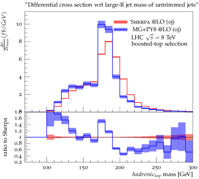
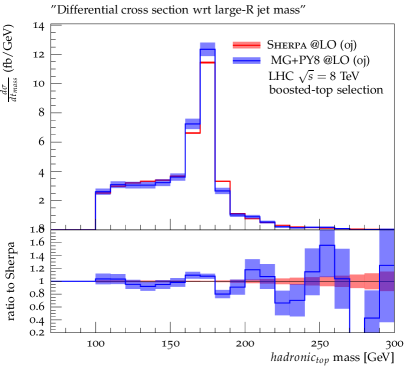
Figure 1: Invariant mass distribution of the hadronic-top candidates in the Boosted event selection. The theoretical predictions from Sherpa and MadGraph_aMCNLO+Pythia8 are based on LO matrix elements dressed with parton showers, left panel without and right panel with applying the trimming procedure.

In Fig. 1 we present the resulting invariant-mass distributions obtained from Sherpa and MadGraph_aMCNLO before and after applying the grooming procedure. Comparing the untrimmed distributions (left panel) both samples exhibit a clear peak at the nominal top-quark mass. However, due to parton-shower radiation and non-perturbative corrections from hadronization and underlying event the peak is rather broad and sizeable differences are observed when comparing the predictions from Sherpa and MadGraph_aMCNLO+Pythia8. Note that the uncertainty bands shown represent the statistical uncertainty of the samples only. When applying the trimming procedure to the had-jet candidates the mass distributions agree to a much better degree, both in the tails of the distribution and the peak region. Therefore, trimming of the large-R jets significantly reduces the dependence on the generator and the details of its parton-shower formalism and the modelling of non-perturbative effects.

In Figs. 2 and 3 we compare predictions from Sherpa based on LO and NLO matrix elements against data measured by the ATLAS experiment for the Boosted (left panels) and the Resolved (right panels) event selections. For the MEPS@LO sample we merge LO QCD matrix elements for $t\bar{t}+0,1,2,3$jet production dressed with the Sherpa dipole parton shower Hoeche:2009rj . The merging-scale parameter is set to $Q_{\rm cut}=20\,{\rm GeV}$. The MEPS@NLO sample combines QCD matrix elements at NLO for $t\bar{t}+0,1$jet and $t\bar{t}+2,3$jets at LO according to the methods described in Hoche:2010kg ; Hoeche:2012yf , again using a merging scale of $Q_{\rm cut}=20\,{\rm GeV}$. Both methods share the event-wise reconstruction of an underlying $jj\to t\bar{t}$ core process through consecutive clusterings of the external legs. For this reconstructed core process the renormalization and factorization scales are set to $\mu_{R}=\mu_{F}=\mu_{\rm core}$, with

$$\mu^{2}_{\rm core}=\frac{1}{4}[m_{t}^{2}+\frac{1}{2}(p_{T,t}^{2}+p_{T,\bar{t}}^{2})]\,.$$ (4)

For the reconstructed clusterings the strong coupling is evaluated at the respective splitting scale. The scale $\mu_{\rm core}$ is furthermore used as the resummation, i.e. parton-shower starting scale, denoted $\mu_{Q}$. To assess the scale uncertainty of the predictions we perform variations by common factors of $2$ and $1/2$ for the core scale and the local splitting scales, using the event-reweighting technique described in Bothmann:2016nao . In the figures the resulting uncertainty estimate is represented by the red band, while the blue band indicates the statistical uncertainty.

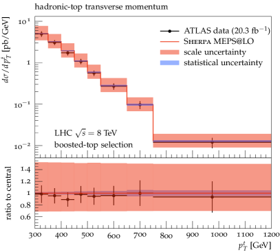
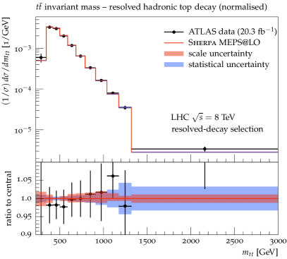
Figure 2: Comparison of predictions based on Sherpa MEPS@LO simulations to data measured by the ATLAS experiment. The left panel shows the $p_{T}$ of the hadronic top in the Boosted selection, data taken from  Aad:2015hna . In the right panel the reconstructed invariant mass of the $t\bar{t}$ system in the Resolved event selection is depicted, with data taken from Aad:2015mbv .

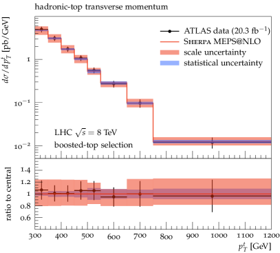
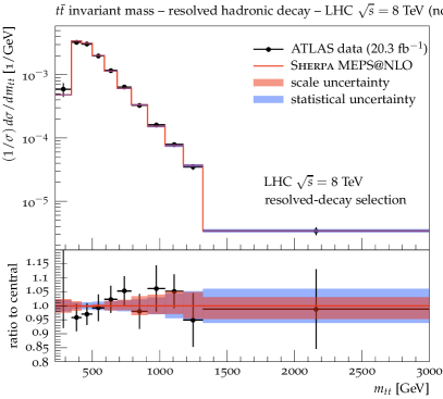
Figure 3: As Fig. 2 but based on Sherpa MEPS@NLO simulations.

For the boosted-top selection we show the transverse-momentum distribution of the hadronic-top candidate in the left panels of Figs. 2 and 3, respectively. Notably, both samples, i.e. the MEPS@LO and the MEPS@NLO prediction, describe the ATLAS measurement Aad:2015hna very well, both in terms of the production rate and in particular concerning the shape of the distribution. For the MEPS@LO result the scale uncertainty is quite significant, reaching up to 50%. However, the dominant effect is a mere rescaling of the total production rate, the shape of the distribution stays almost unaltered. This is also observed for the MEPS@NLO sample, however, the scale uncertainty reduces to $\pm 20\%$.

For the resolved-decay selection we compare the Sherpa MEPS@(N)LO predictions for the reconstructed invariant mass of the $t\bar{t}$ system against data from the ATLAS experiment Aad:2015mbv , see right panels of Figs. 2 and 3. Note that the data and the theoretical predictions are normalized to their respective fiducial cross section. The MEPS@LO and MEPS@NLO results agree very well with the data. For this normalized distribution the scale uncertainties largely cancel. For the MEPS@LO sample this results in an uncertainty estimate of $\pm 2\%$. For the MEPS@NLO sample the shape modifications induced by the scale variations amount to $\pm 5\%$.

For both observables considered, the MEPS@(N)LO predictions from Sherpa yield a very satisfactory description of the data. No significant alteration of the distributions shape is observed upon inclusion of the QCD one-loop corrections in the MEPS@NLO sample. However, in particular the uncertainty on the production rate reduces significantly. For the normalized top-pair invariant mass distribution we consider the more realistic $\pm 5\%$ estimate from the MEPS@NLO calculation. By normalizing the distribution to the cross section in a certain mass window, this uncertainty might in fact be reduced further, cf. Ref. Czakon:2016vfr , where, ultimately, an uncertainty estimate of ${\cal{O}}(1\%)$ was quoted for the corresponding NNLO QCD prediction.

In what follows we want to study the imprint of New Physics resonant contributions on the top-pair invariant mass distribution. To this end we currently rely on a leading-order description of the signal, interfering with the corresponding SM amplitudes. However, from the considerations above we can conclude that the MEPS@LO calculation of the SM production process captures the dominant QCD corrections, which are of real-radiation type. To illustrate this further, we present in Fig. 4 a comparison of MEPS@LO samples using different parton-multiplicity matrix elements for the mass and the transverse momentum of the $t\bar{t}$ system in the Boosted selection. These results get compared to the corresponding MEPS@NLO prediction described above.

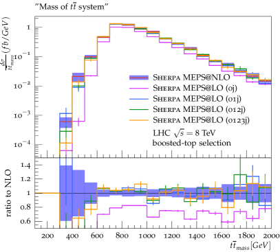
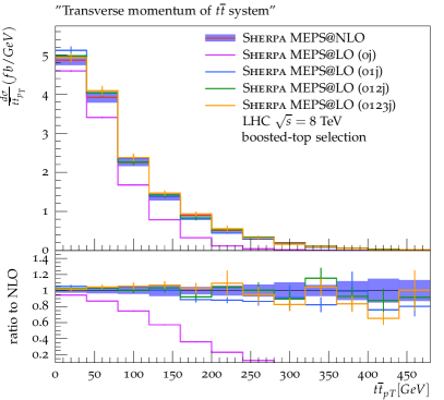
Figure 4: Comparison of MEPS@LO predictions based on different maximal parton-multiplicity matrix elements and the MEPS@NLO calculation for the Boosted event selection. The left panel shows the top-pair invariant mass, the right panel the transverse momentum of the $t\bar{t}$ system.

For the top-pair invariant mass all the predictions with at least one extra hard jet agree within their statistical errors. In particular, even the MEPS@LO sample, based on merging the LO matrix elements for $t\bar{t}+0,1$jet only, well reproduces the MEPS@NLO result and greatly improves the 0jet sample. As might be expected, for the transverse momentum of the $t\bar{t}$ system, the inclusion of higher-multiplicity matrix elements improves the agreement with the MEPS@NLO result. The MEPS@LO calculation based on $t\bar{t}+0,1$jet predicts a somewhat softer spectrum, i.e. is lacking configuration corresponding to multiple hard emissions. However, the bulk of the events in the Boosted selection is reasonably modeled by this simple LO merging setup and describes the data presented above very well. We will therefore rely on this setup when invoking New Physics contributions.

In the following we also introduce a simple Parton Analysis, used to quantify the effect of the NP without any smearing due to the reconstruction of the top quarks. In the Parton Analysis no cuts are applied to the events and the two top quarks are identified, before any decay, using truth-level information from the generator.

IV Simplified model

Several models of NP predict resonances decaying to top-quarks. Scalar resonances in particular have large branching ratios in this decay channel due to the fact that their couplings with fermions are often proportional to the fermion masses. In this case, the resonance is at the LHC dominantly produced via gluon fusion through loops of colored particles. These colored particles can be either light compared to the resonance (like the top quark itself), in which case the structure of the loop is resolved as illustrated in Fig. 5(a), or they can be heavy, in which case a point-like interaction sketched in Fig. 5(b) can describe the interactions.

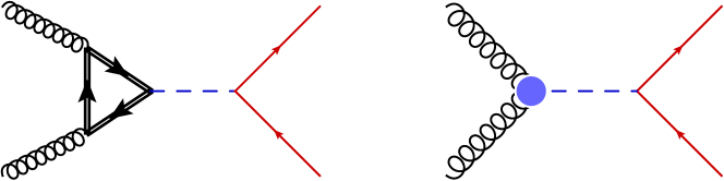
(a)                                                          (b)

Figure 5: Feynman diagrams for production of a scalar resonance with subsequent decay into top-quarks, mediated by a resolved loop (a) or via high-scale New Physics (b).

It has been shown in Manohar:2006ga that the most general scalar extension of the SM which couples to fermions and maintains naturally small flavour changing neutral currents is provided by scalars with the same quantum numbers of the Higgs doublet or that transform as a color octet $(\bf 8,2)_{1/2}$ under the SU(3)$\times$SU(2)$\times$U(1) SM gauge group. Color neutral and octet scalars arise also naturally in several models of dynamical EWSB, such as in the seminal Farhi-Susskind model Farhi:1980xs and models where the top is partially composite Belyaev:2016ftv . Although the specific origin of the scalar-top couplings is important, determining the relation to other couplings and their magnitudes, we here adopt a more phenomenological simplified approach relevant for top-quark pair production, in which the left-handed top is stripped off from its doublet and couples directly to the scalars.

In our simplified model we assume the only light state running in the loop to be the top-quark. This is a good approximation if two conditions are fulfilled: (i) - the bottom-quark contribution is suppressed; and (ii) - the extra states contributing significantly to the gluon–scalar couplings are heavy (at least as much as the scalar resonance itself). This is a good approximation in many models beyond the SM. In the THDM Branco:2011iw for example, there is no new particle living at higher scale apart from the new scalar sector. Moreover, the loop of bottom-quarks is usually suppressed in the cases relevant for $t\bar{t}$ production. Specializations of the THDM such as the Minimal Supersymmetric Standard Model (MSSM) where the super-partners are heavy enough to be integrated out can also be described in this framework. Composite models typically predict relatively degenerate spectra of first excitations, thus they can be usually described by the effective point-like interaction. Similarly, for the color octet in the model of Manohar and Wise Manohar:2006ga the scalars are produced purely by top and bottom loops. In some other models intermediate states much lighter than the first scalar excitations are present, e.g. top partners and stops may be light in some models of partial compositeness and SUSY – in these cases our approximation is not applicable.

Under this assumption we can describe the scalar sector interactions relevant for $t\bar{t}$ production via the following Lagrangian:

$$\mathcal{L}_{\phi} = ic^{\eta}_{t}\frac{m_{t}}{v}\bar{t}\gamma_{5}t\eta+c^{\sigma}_{t}\frac{m_{t}}{v}\bar{t}t\sigma+ic^{\tilde{\eta}}_{t}\frac{m_{t}}{v}\bar{t}\gamma_{5}\frac{\lambda^{a}}{2}t\tilde{\eta}^{a}+c^{\tilde{\sigma}}_{t}\frac{m_{t}}{v}\bar{t}\frac{\lambda^{a}}{2}t{\tilde{\sigma}}^{a}$$ (5)

$$+ c_{g}^{\sigma}\frac{\alpha_{S}}{12\pi v}\sigma G^{a}_{\mu\nu}G^{a\mu\nu}-c_{g}^{\eta}\frac{\alpha_{S}}{8\pi v}\eta G^{a}_{\mu\nu}\widetilde{G}^{a\mu\nu}$$

$$- c_{g}^{\tilde{\eta}}\frac{\alpha_{S}}{8\pi v}\tilde{\eta}^{a}d^{abc}\widetilde{G}^{a\mu\nu}G^{b\rho\sigma}+c_{g}^{\tilde{\sigma}}\frac{\alpha_{S}}{12\pi v}{\tilde{\sigma}}^{a}d^{abc}\widetilde{G}^{a\mu\nu}G^{b\rho\sigma}\,.$$

It contains a CP-odd isosinglet scalar $\eta$, a CP-even isosinglet scalar $\sigma$, a CP-odd color octet scalar $\tilde{\eta}$ and a CP-even octet scalar $\tilde{\sigma}$ which we collectively call $\phi$. $G^{\mu\nu}$ is the gluon field-strength tensor, $\widetilde{G}^{\mu\nu}=\frac{1}{2}\epsilon^{\mu\nu\rho\sigma}G_{\rho\sigma}$, $\lambda^{a}$ are the SU(3) generators and $d^{abc}=\frac{1}{4}Tr[\lambda^{a}{\lambda^{b},\lambda^{c}}]$ is the fully symmetric SU(3) tensor.

The top-quark loops generate form factors that describe the gluon-scalar interaction. The loop triangles contribute to the trilinear $gg\phi$ vertices in the form

$$\eta g_{a}^{\mu}(k_{1})g_{b}^{\nu}(k_{2}) : \quad\frac{\alpha_{S}c_{t}^{\eta}}{2\pi v}A^{A}_{1/2}\left(\frac{s}{4m_{t}^{2}}\right)\epsilon^{\mu\nu\lambda\sigma}k_{1\lambda}k_{2\sigma}\delta_{ab}\,,$$ (6)

$$\sigma g_{a}^{\mu}(k_{1})g_{b}^{\nu}(k_{2}) : \quad\frac{\alpha_{S}c_{t}^{\sigma}}{3\pi v}A^{S}_{1/2}\left(\frac{s}{4m_{t}^{2}}\right)(k_{1}^{\nu}k_{2}^{\mu}-k_{1}\cdot k_{2}g^{\mu\nu})\delta_{ab}\,,$$ (7)

with

$$A^{A}_{1/2}(\tau) = f(\tau)/\tau\,,$$ (8)

$$A^{S}_{1/2}(\tau) = \frac{3}{2\tau^{2}}\left(\tau+(\tau-1)f(\tau)\right)\,,$$ (9)

$$f(\tau) = \begin{cases}\text{arcsin}^{2}(\sqrt{\tau}),&\quad\tau\leq 1\\ -\frac{1}{4}\left[\log\left(\frac{1+\sqrt{1-\tau^{-1}}}{1-\sqrt{1-\tau^{-1}}}\right)-i\pi\right]^{2},&\quad\tau>1\,.\end{cases}$$ (10)

Similar expressions for the color octet top-quark loop generated form factor can be found e.g. in Hayreter:2017wra .

As a matter of fact, resonant top pair production is accompanied by other signatures. In particular, diphoton, dijet, $\gamma Z$, $ZZ$ and $W^{+}W^{-}$ signatures are generated via diagrams induced by a top-quark loop, and in general by high-scale physics. Tree-level $ZZ$, $W^{+}W^{-}$ decay channels are typically present for a scalar state, while decays into lighter fermions are typically suppressed. Color octets decays into $g\gamma$ and $gZ$ might give striking signatures. The detailed analysis of these channels is not in the scope of this work, however, we provide some qualitative discussion about the regions in parameter space where they can be competitive in sensitivity to $t\bar{t}$ search.

Loop (or anomaly) induced decays are typically suppressed and might be competitive to $t\bar{t}$ searches only for small Yukawa couplings $c_{t}$. They are often the only possible decay channels for pseudo-scalars besides that into $t\bar{t}$. As an example, consider some partial widths of a color-singlet pseudo-scalar

$$\Gamma_{\eta\to t\bar{t}} = \frac{3}{8\pi}\frac{m_{t}^{2}}{v^{2}}(c^{\eta}_{t})^{2}\,m_{\eta}\sqrt{1-4m_{t}^{2}/m_{\eta}^{2}}\,,$$ (11)

$$\Gamma_{\eta\to gg} \simeq \frac{\alpha_{s}^{2}m_{\eta_{X}}^{3}}{32\pi^{3}v^{2}}\left|c_{t}^{\eta}A^{A}_{1/2}\left(\frac{m_{\eta}^{2}}{4m_{t}^{2}}\right)+c_{g}^{\eta}\right|^{2}\,,$$ (12)

$$\Gamma_{\eta\to\gamma\gamma} \simeq \frac{\alpha^{2}m_{\eta_{X}}^{3}}{256\pi^{3}v^{2}}\left|c_{t}^{\eta}3(2/3)^{2}A^{A}_{1/2}\left(\frac{m_{\eta}^{2}}{4m_{t}^{2}}\right)+c_{\gamma}^{\eta}\right|^{2}\,.$$ (13)

Here we parametrize the photon interaction with $\eta$ by the following gauge invariant operators

$$\mathcal{L}_{\phi,\gamma}=-c_{W}^{\eta}\frac{\alpha}{8\pi v}\eta W^{i}_{\mu\nu}\widetilde{W}^{i\mu\nu}-c_{B}^{\eta}\frac{\alpha}{8\pi v}\eta B_{\mu\nu}\widetilde{B}^{\mu\nu}\,,$$ (14)

with $c_{\gamma}^{\eta}\equiv c_{W}^{\eta}+c_{B}^{\eta}$. These operators also give rise to decays into weak bosons, but not competitive in sensitivity to diphoton searches (unless there is some cancellation in $c_{W}+c_{B}$). From the above expressions it can be noticed that the $gg$ partial width is much larger than $\gamma\gamma$, however, the corresponding search is not as competitive to the diphoton channel due to the clean signature of the latter.

On the other hand, scalar resonances tend to decay into weak bosons at tree level, with large contributions to their decay width and good sensitivity in the corresponding channels.

The color octets have more unexplored signatures, like e.g. $g\gamma$, studied for example in Ref. Aad:2015ywd ; Aaboud:2017nak .

IV.1 Model description and simulation

Our goal is to achieve accurate predictions for a wide parameter range of our generic model in an efficient and fast way. For this purpose, the Lagrangian given in eq. (5) has been implemented into the FeynRules Alloul:2013bka package to produce a corresponding UFO model file Degrande:2011ua . The required helicity amplitudes have been extracted to C++ codes via the Madgraph Alwall:2011uj program and incorporated in the Rivet  analyses in order to perform a reweighting method and reproduce the signal line-shape. To this end, each event of the Sherpa SM event sample is given a weight, $w$, proportional to the ratio of the amplitudes,

$$w=\frac{\overline{|\mathcal{M}_{\rm SM}+\mathcal{M}_{\phi}|^{2}}}{\overline{|\mathcal{M}_{\rm SM}|^{2}}},$$ (15)

where $\overline{|\mathcal{M}_{\rm SM}|^{2}}$ is the SM amplitude squared summed and averaged over color and spin. In the numerator the amplitude $\mathcal{M}_{\phi}$ corresponding to the resonant diagrams depicted in Fig. 5 is added on top of the SM diagrams. The further decay of top quarks is included neglecting non-resonant diagrams. Therefore, the full process in eq. (1) – including possible extra hard radiation – is considered with full spin correlation of the top-quark decays.

We note that our signal includes not only the purely resonant contribution. The complete squared amplitude can be split into three contributions:

$$|\mathcal{M}_{\rm SM}+\mathcal{M}_{\phi}|^{2}=|\mathcal{M}_{\rm SM}|^{2}+|\mathcal{M}_{\phi}|^{2}+2{\rm Re}\,\mathcal{M}_{\rm SM}^{*}\mathcal{M}_{\phi}\equiv B_{\mathcal{M}}+S_{\mathcal{M}}+I_{\mathcal{M}}\,.$$ (16)

The last term defines the SM background ($B_{\mathcal{M}}$), the pure signal ($S_{\mathcal{M}}$) and the interference between signal and SM ($I_{\mathcal{M}}$).

We use as the test observable the $m(t\bar{t})$ distribution of the signal hypothesis $H$ normalized bin-by-bin to the SM QCD prediction,

$$r(H)\equiv\frac{d\sigma_{H}/dm}{d\sigma_{\rm SM}/dm}\,.$$ (17)

The signal hypothesis differential cross section $d\sigma_{H}/dm$ is defined as the total differential cross section subtracted by the SM prediction. Such normalized distribution is less affected by systematic errors, i.e. theoretical uncertainties Czakon:2017wor .

In order to assess the importance of the interference we study both the full signal including interference $d\sigma_{S+I}/dm$ and the pure signal hypothesis neglecting interference $d\sigma_{S}/dm$. To simplify the notation in the remaining of the text we use the following definitions:

$$d\sigma_{S}/dm\equiv S_{\sigma},\quad d\sigma_{I}/dm\equiv I_{\sigma},\quad d\sigma_{\rm SM}/dm\equiv B_{\sigma}\,.$$ (18)

Interference between signal (Fig. 5) and QCD diagrams are known to be important in this process. In fact, they can completely change the line-shape of the resonance from a pure Breit-Wigner peak to a peak-dip structure, or even dip-peak, pure dip or an enhanced peak Gaemers:1984sj ; Dicus:1994bm ; Frederix:2007gi ; Gori:2016zto ; Jung:2015gta ; Djouadi:2016ack . QCD corrections to this effect have recently been computed Bernreuther:2015fts ; Hespel:2016qaf ; BuarqueFranzosi:2017jrj and shown to be important. A pilot experimental analysis investigating such interference effects has been presented recently Aaboud:2017hnm .

The form factors in eq. (7) have been implemented in the helicity amplitudes used in the reweighting step. However, the corresponding box diagram contributing to the four-gluon–scalar coupling was kept as an effective vertex without momentum dependence. For the color octet the form factor is approximated by a fixed momentum flowing through the loop that is equal to the mass of the resonance. The interference between top-quark loops and point-like interactions is also manifest in the calculation.

Higher-order QCD corrections are partially taken into account through the radiation of extra gluons in the MEPS@LO simulation. The contribution from real-emission $t\bar{t}j$ matrix elements also get reweighted with the NP theory hypotheses.

We note however that the method neglects the signals’ color-singlet color flow contribution when attaching parton showers, which affects the subsequent radiation pattern only. We nevertheless found that these effects are small in the description of the top-pair mass distribution. In Fig. 6 we show the distribution of variable $r(S)$ defined in eq. (17) for a color-singlet pseudo-scalar of mass $1.5$ TeV in the pure signal hypothesis, comparing the Sherpa reweighted events with a dedicated simulation of the full process with MadGraph_aMCNLO+Pythia8. In the latter, the color-flow contribution corresponding to the signal diagrams are considered as seeds for the subsequent parton shower. The error near the resonance peak is about 10% and the reweighted prediction underestimates the yields. We removed the top-quark loop form factor considering only the effective scalar-gluon coupling for this comparison. The distributions were derived according to the Parton Analysis framework described in sec. (III). In the more realistic boosted analysis we expect the reweighting method to predict a more smeared distribution due to the extra connected color lines that favor extra hard radiation connecting the top quarks with initial gluons. We will neglect these effects and employ the reweighting method in what follows to make predictions for a large region of parameter space of the model, while avoiding massive time and machine consuming event generation and “fake” MC statistical error. Our results are expected to give conservative limits since for colour-singlet resonances the signal color flow induces less smearing of the resonance peak.

Figure 6: Comparison of the predictions for the top-pair invariant mass from the reweighting method (Sherpa+ RW) and a dedicated full simulation with MadGraph_aMCNLO+Pythia8 for a color-singlet pseudo-scalar of mass $m=1.5$ TeV. The Parton Analysis was adopted.

V Results

Resonant top-quark pair production at the LHC has been analyzed for several of the models mentioned above already. Color neutral resonances decaying into $t\bar{t}$ have been studied in several works for a large number of models Gaemers:1984sj ; Dicus:1994bm ; Gori:2016zto ; Jung:2015gta ; Djouadi:2016ack , even including interference effects at NLO in QCD Bernreuther:2015fts ; Hespel:2016qaf ; BuarqueFranzosi:2017jrj . The case of a color-octet signal has been considered in Frederix:2007gi ; FileviezPerez:2008ib ; Frolov:2016gvu ; Hayreter:2017wra , also considering other production channels, e.g. via $b\bar{b}$ initial states, or even double scalar production Gerbush:2007fe ; Kim:2008bx ; Schumann:2011ji . Our approach differs from previous studies because we adopt the strategy of directly comparing to data which has been shown to agree well with the SM prediction, and therefore, can be used to put direct limits on the model parameters, in the same spirit as Butterworth:2016sqg . Indeed, the recent ATLAS measurement of the top-quark pair differential cross section at $\sqrt{s}=13\,\text{TeV}$ shows good agreement with various SM Monte Carlo generators Aaboud:2017fha . However, there are no measurements of the $t\bar{t}$ invariant mass in the boosted regime at this energy yet. Moreover, the uncertainties are still quite large, since only the 2015 data, corresponding to $3.2\,{\rm fb}^{-1}$, were used, but we expect that an update of the analysis will be available in the near future, with improved systematics and statistical uncertainty (comparable to the ones presented in this paper) allowing to derive real exclusion limits. We assume in what follows that data will be well described by the SM expectation, and take the SM prediction from Sherpa  as mock data.

The method proposed allows theorists to derive realistic exclusion limits on a variety of NP scenarios without a dedicated and expensive experimental analysis. It opens a new path to search for NP, with the experiments providing precision measurements of SM processes. With respect to dedicated experimental searches, it can serve as check and as an alternative (less-expensive) approach to look for more general parametrizations of deviations caused by New Physics. For instance, in the ATLAS and CMS collaborations’ analyses Khachatryan:2015sma ; Chatrchyan:2013lca ; Chatrchyan:2012cx ; Sirunyan:2017uhk ; Aaboud:2017hnm , only a leptophobic Z’ bosons (present for instance in topcolor scenarios), a Kaluza-Klein excitation of the gluon and heavy states in THDM were searched for. Moreover, interference effects were considered only in Ref. Aaboud:2017hnm . With our technique we are able to provide limits for a whole wealth of models.

In order to assess the possibility to observe the signals described above we perform a simple $\chi^{2}$ analysis using the bins of the $r$ distribution. We consider the mass window $m_{\phi}-200\,{\rm\,\text{GeV}}<m(t\bar{t})<m_{\phi}+200\,{\rm\,\text{GeV}}$ and compute

$$\chi^{2}_{N}=\sum_{i=1}^{N}\frac{r_{i}(H)^{2}}{\sigma_{i}^{2}}\,,$$ (19)

with $N$ the number of bins taken into account, according to the assumed resolution of the measurement. $r_{i}(H)$ is the $r(H)$ distribution integrated over bin $i$ and $H$ is the hypothesis (either $S$ or $S+I$). $\sigma^{2}_{i}$ is the variance on each bin of the distribution.

The variance is derived according to the rules of propagation of uncertainties and is estimated by

$$\sigma^{2}=\frac{1}{B_{\sigma}}\left(1+\frac{H_{\sigma}^{2}}{B_{\sigma}^{2}}\right)+\epsilon_{\rm SYS}^{2}\left(1+\frac{H_{\sigma}^{2}}{B_{\sigma}^{2}}\right)+\epsilon_{\rm TH}^{2}\frac{(H_{\sigma}+B_{\sigma})^{2}}{B_{\sigma}^{2}}\,.$$ (20)

We kept the indexes $i$ implicit in the expression. The first term accounts for statistical error, the second for systematic uncertainties of experimental sources, and the third for theoretical uncertainties. We assume a flat distribution for theory and systematic uncertainty, and that statistical uncertainties are dominated by the background, with a small ratio signal over background. We take $\epsilon_{TH}=1\%$ for both $H_{\sigma}=S_{\sigma}$ and $H_{\sigma}=S_{\sigma}+I_{\sigma}$, assuming other errors are strongly correlated and will be canceled when taking the ratio distribution. The experimental uncertainty is more important and we consider three benchmark estimates for $\epsilon_{\rm SYS}$:

1. In Ref. Aaboud:2017hnm the total systematics on the background were estimated as 10% and 11%. As a pessimistic case we consider $\epsilon_{\rm SYS}=10\%-15\%$.

2. As an optimistic scenario we vary it to lower values considering a future improved understanding of the uncertainties and the reduction in uncertainty associated to normalization. Since we are using a normalized distribution many of the uncertainties estimated in the previous benchmark are strongly correlated and will be canceled out. For this we use $\epsilon_{\rm SYS}=5\%-10\%$.

3. As the most optimistic case we assume experimental uncertainties can be drastically reduced to the level of theoretical, which according to Ref. Czakon:2017wor results in $\epsilon_{\rm SYS}=1\%-2\%$.

We consider $N=1$ for a bad resolution case, assuming the experiment can resolve only the full window of 400 GeV in $m(t\bar{t})$, and $N=10$ assuming a mass resolution in $m(t\bar{t})$ of $40$ GeV.

We consider $\chi^{2}\geq 2$ as a criterion for exclusion, which corresponds roughly to an exclusion at 95% of confidence level.

This simple analysis is intended to be a first approximation to a full statistical data analysis that will be carried out eventually. In particular we assume the same uncertainty for every bin without correlation between them, and we assume only two cases of resolution independent of the bin. In the following we discuss some benchmark scenarios and the respective results.

V.1 Pseudo-scalar color octet

The first scenario we consider is when the resonance $\phi$ represents a pseudo-scalar color octet ($\widetilde{\eta}$) with total width dominated by the decays to pairs of tops and gluons

$$\Gamma_{\rm TOT}=\Gamma_{tt}+\Gamma_{gg}\,.$$ (21)

In Fig. 7 we show the resulting $r$ distribution assuming a color octet resonance with mass $m_{\tilde{\eta}}=500$ GeV and the parameters $c_{t}=1$, $c_{g}=1$ (left) and $c_{g}=-1$ (right) at parton level, i.e. using the Parton Analysis described in sec. (III). We show both the full line-shape, which comprises signal and interference with QCD background (S+I), and the pure signal (S) for comparison. The importance of taking into account interference effects can clearly be noticed.

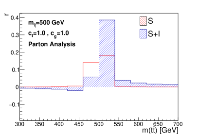
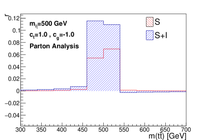
Figure 7: Normalized top-pair mass distributions, $r\equiv\frac{d\sigma/dm}{d\sigma_{\rm SM}/dm}$ for a pseudo-scalar color octet resonance with $m_{\tilde{\eta}}=500\,{\rm\,\text{GeV}}$, $c_{t}=1$ and $c_{g}=1$ ($c_{g}=-1$) on the left (right) using the Parton analysis. Signal plus interference (S+I) is in blue and pure signal (S) in red.

Similarly, in Fig. 8, we present the effect of a resonance with mass $m_{\tilde{\eta}}=1700\,{\rm GeV}$ and couplings $c_{t}=1$, $c_{g}=1$ (left) and $c_{g}=-1$ (right), reconstructed using the Boosted Analysis. The excess reaches more than 10%, which indicates that even a pessimistic estimate of the uncertainties is sufficient to exclude the existence of this state for values of $c_{g}$ of order 1. We thus use the most pessimistic value for the systematic error, $\epsilon_{\rm SYS}=10\%-15\%$.

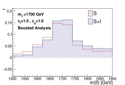
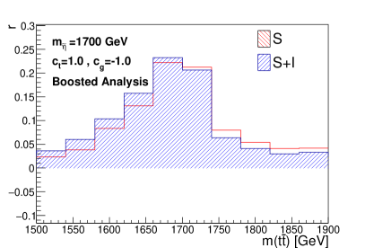
Figure 8: Normalized top-pair mass distributions $r$ reconstructed with the Boosted analysis for a pseudo-scalar color octet resonance with $m_{\tilde{\eta}}=1700\,{\rm\,\text{GeV}}$, $c_{t}=1$ and $c_{g}=1$ ($c_{g}=-1$) on the left (right). The color scheme is the same as in Fig. 7.

In Fig. 9 the corresponding exclusion limits are shown, assuming a fixed value of $c_{t}=1$. The bands correspond to a systematic uncertainty on the measurement running from $10\%$ to $15\%$. The limits are evaluated considering the interference effect (dashed lines) or neglecting it (continuous lines). The interference has a significant effect in the low mass region ($m_{\tilde{\eta}}<1.3\,{\rm TeV}$). The excluded region corresponds to larger values of $|c_{g}|$. We show the exclusion for integrated luminosities of $L=20\,{\rm fb}^{-1}$ (blue line) and $L=100\,{\rm fb}^{-1}$ (black). In the left-panel we use $10$ bins of $40\,{\rm GeV}$ width in the invariant-mass distribution to compute $\chi^{2}_{10}=2$ while on the right-panel we use only a single 400 GeV bin centered around the resonance mass, $\chi^{2}_{1}=2$. The comparison between the left and right panel shows the importance of a good resolution and for a line-shape analysis.

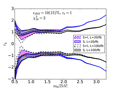
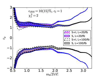
Figure 9: Exclusion limits ($\chi^{2}=2$) in $(m_{\tilde{\eta}},c_{g})$ parameter space for a pseudo-scalar color octet assuming $c_{t}=1$. The band represents the different assumptions for the systematic uncertainty, varying from 10% to 15%. Integrated luminosities are $L=20\,{\rm fb}^{-1}$ (blue line) and $L=100\,{\rm fb}^{-1}$ (black), as well as considering interference (dashed line) and neglecting it (solid line).

We expect striking signatures in other channels, but little has been studied. For instance, in the analysis of $\gamma$+jets in Ref. Aaboud:2017nak a color octet has not been considered.

V.2 Pseudo-scalar singlet

For the benchmark scenario of a pseudo-scalar color singlet we again assume the resonance’ width is dominated by the top and gluon decays, as in eq. (21).

We show in Fig. 10 the distribution of the normalized $m(t\bar{t})$ distribution $r$ assuming $m_{\eta}=1500\,{\rm GeV}$. In the left-hand (right-hand) panel we consider $c_{g}=1$ ($c_{g}=-1$). The line-shapes of this scenario are highly non-trivial, they strongly depend on the mass and couplings, and can feature pure dips, pure peaks and intermediate peak-dip or dip-peak structures. A sample of different line-shapes is shown in app. (A).

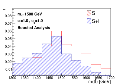
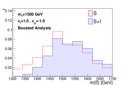
Figure 10: Normalized top-pair mass distributions $r$ reconstructed with the Boosted analysis for a pseudo-scalar color singlet resonance with $m_{\eta}=1500\,{\rm\,\text{GeV}}$, $c_{t}=1$ and $c_{g}=1$ ($c_{g}=-1$) on the left (right). The color-scheme is the same as in Fig. 7.

In Fig. 11 we show the exclusion limits in the $(m_{\eta},c_{g})$ parameter space plane for $c_{t}=1$. The band represents the different assumptions for the systematic uncertainty, 5% and 10%. The effect of interference is important for low masses $m_{\eta}\lesssim 1.2\,{\rm\,\text{TeV}}$, where also systematics dominate and have a huge impact on the exclusion power. The use of the full line-shape in the statistical analysis improves the exclusion power mostly for low masses where more distinct line-shapes are present. For masses above $m_{\eta}\gtrsim 2\,{\rm\,\text{TeV}}$, higher luminosities than $L=100\,{\rm fb}^{-1}$ are needed.

In Fig. 12 we show the corresponding exclusion limits in the $(c_{t},c_{g})$ plane for a fixed mass $m_{\eta}=1.5\,{\rm\,\text{TeV}}$. The effect of interference is important for large top couplings, $c_{t}\gtrsim 1.2$, which is directly related to the size of the width. The use of full line-shape gives a mild improvement in the exclusion power.

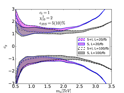
Figure 11: Exclusion limits ($\chi^{2}=2$) in $(m_{\eta},c_{g})$ parameter space and $c_{t}=1$ for a pseudo-scalar color singlet. The band represents the different assumptions for the systematic uncertainty, varying from 5% to 10%. The color and style scheme for the lines are the same as in Fig. 9.

Figure 12: Equivalent to Fig. 11 for the $(c_{t},c_{g})$ plane for a fixed mass of $m_{\eta}=1.5\,{\rm\,\text{TeV}}$

For very low masses the Resolved analysis can be slightly more powerful than the Boosted. In Fig. 13 on the left we show an example of a line-shape and on the right the exclusion limit provided by the Resolved analysis. Compared to fig. (11) it can be noticed that the low mass region $m_{\eta}\lesssim 600\,\text{GeV}$ can be better covered by the Resolved selection. We note as well that the case of negative $c_{g}$ is less excluded due to the fact that larger cancellations between top-quark loop and effective vertex happens for these masses.

Figure 13: Left: Normalized top pair mass distributions $r$ for $c_{g}=c_{t}=1$ and $m_{\eta}=500\,{\rm\,\text{GeV}}$. Right: Exclusion limit ($\chi^{2}=2$) in $(m_{\eta},c_{g})$ parameter space for $c_{t}=1$. The color scheme is the same as in Fig. 11. In both panels the Resolved analysis has been employed.

Diphoton and dijet searches might be relevant in extreme regions of parameter space, i.e. for very small $c_{t}\sim 0.2$, and large masses, due to the dependence of the $\gamma\gamma$ and $gg$ partial widths on $m^{3}$ as opposed to the linear dependence of the $t\bar{t}$ decay width. In fig. (14) we show the 95%CL excluded region derived from the limits provided by the ATLAS collaboration in the dijet search Aaboud:2017yvp . We used the case $\sigma_{G}/m_{G}=0$ and assumed an acceptance of 50%. In the same figure we show the 95%CL excluded region in the diphoton channel using the exclusion limits by the ATLAS analysis in Ref. Aaboud:2017yyg . We used the case $\Gamma_{X}/M_{X}=6\%$ and the spin-0 selection. To derive cross sections we used the N³LO result for Higgs production cross section $\sigma_{h}$ Anastasiou:2016hlm and rescale by the LO decay width,

$$\sigma_{\eta}=\sigma_{h}\frac{\Gamma_{\eta\to gg}}{\Gamma_{h\to gg}}=\sigma_{h}\frac{\left|c_{t}^{\eta}A^{A}_{1/2}\left(\frac{m_{\eta}^{2}}{4m_{t}^{2}}\right)+c_{g}^{\eta}\right|^{2}}{\left|A^{S}_{1/2}\left(\frac{m_{\eta}^{2}}{4m_{t}^{2}}\right)\right|^{2}}.$$ (22)

$\Gamma_{\eta\to gg}$ is given in eq. (13) and the form factors in eqs. (8–10). The shaded area in the figure represents the region where $\sigma_{\eta}\times$BR is larger than the excluded line in the respective references, and BR is the corresponding branching ratios. We can notice that these channels get competitive in sensitivity to $t\bar{t}$ analysis at low $c_{t}$ and large mass, but only if $c_{\gamma}$ is particularly large. In particular, even for $c_{t}=1$, for $m>3\,\text{TeV}$ the dijet search seems to be more sensitive to New Physics.

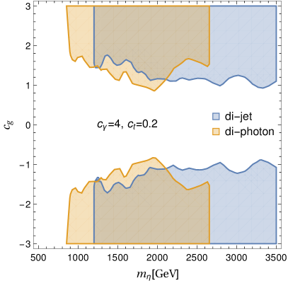
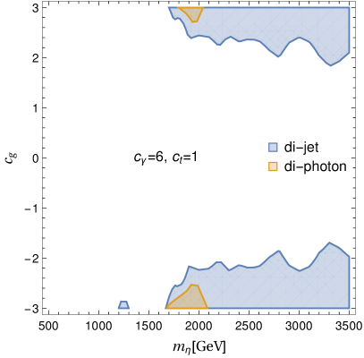
Figure 14: 95%CL excluded region in parameter space in diphoton Aaboud:2017yyg and dijet searches Aaboud:2017yvp . On the left panel $c_{\gamma}=4$ and $c_{t}=0.2$. On the right, $c_{\gamma}=6$ and $c_{t}=1$.

Interpretation for Composite Higgs models with Top Partial Compositeness

As an ultra-violet realization of the pseudo-scalar scenario we consider the composite models M3, M8 and M9 of Ref. Belyaev:2016ftv . These models are constituted by two additional confining fermions, $\psi$ and $\chi$, which form several composite states among which a top partner that can generate a mass to the top quarks through the partial-compositeness mechanism. In addition, they present two iso-singlet pseudo-scalar mass eigenstates $a$ and $\eta^{\prime}$. In general, the observation of such pseudo-scalar state decaying into top quarks can shed light on the mechanism of fermion mass generation Alanne:2016rpe . These models present extra parameters which determine the couplings, given by a pair of integers $(n_{\psi},n_{\xi})$ and the relation between the mixing angle $\alpha$ and the ratio of scales and U(1) charges, $\zeta$. We do not enter a discussion of the details of these the models and their parameters here but invite the reader to consult Ref. Belyaev:2016ftv . We choose $\alpha=\zeta$ and the values of $(n_{\psi},n_{\xi})$ which provide the largest couplings to the tops, $(n_{\psi},n_{\xi})=(2,0),\,(-4,2)$ and $(4,2)$. We neglect contributions to the resonance width from the decays into $Z$, $W$ and $\gamma$, which are sub-dominant. The relevant couplings are summarized in Tab. 2.

Table 2: Summary of the couplings of pseudo-scalar color-singlet state $a$ in the considered composite models. $c_{t}$ and $c_{g}$ are given in units of $v/F_{\pi}$. $c_{t}$ is shown for the three benchmarks $(n_{\psi},n_{\xi})=(2,0)/(-4,2)/(4,2)$.

model	$\quad c_{t}[v/F_{\pi}]\quad$	$c_{g}[v/F_{\pi}]$
M3	0.934/1.09/-2.65	5.44
M8	0.926 /1.54/-2.16	1.54
M9	0.293/-0.195/-1.37	8.6

In Fig. 15 we show the value of $c_{t}$ and $c_{g}$ for each model together with the exclusion region (above the black curve) for a fixed mass $m_{a}=1.5\,{\rm\,\text{TeV}}$. We consider an integrated luminosity of $L=20\,{\rm fb}^{-1}$ for the exclusion limit and a systematic error $\epsilon_{\rm SYS}=5\%$. The different line colors in the figure refer to the different models: red is M8, yellow M9 and brown M3. The styles of the lines represent the fermionic charges: $(n_{\psi},n_{\xi})=(2,0)$ (solid line), (-4,2) (dashed) and (4,2) (dot-dashed). Each line scans the values of $F_{\pi}$ from $v$ (most external and largest couplings) to $8v$ (most internal and smallest couplings), the dots represent the values $F_{\pi}=n\,v$, with $n$ an integer between 1 and 8 included. Also shown for reference in the upper region the couplings of the $\eta_{63}$ state of the Fahri-Susskind one-family model Farhi:1980xs .

From the figure we can get the minimal value of the compositeness scale $F_{\pi}>F_{\pi}^{min}$ for which state $a$ would still not have been observed for different scenarios. For instance, for model M8 (red lines), $v\lesssim F_{\pi}^{min}\lesssim 2v$ depending on the values of $(n_{\psi},n_{\xi})$. The model M3 is more constrained, and $6v\lesssim F_{\pi}^{min}\lesssim 7v$ for (-4,2) and $F_{\pi}^{min}\sim 5v$ for (2,0) or (4,2). Model M9 has low values of $c_{t}$ but values $F_{\pi}\gtrsim 6v$ can be excluded for the case (-4,2), while the other scenarios are hard to access in the $t\bar{t}$ search.

Other decay channels have been analyzed in Ref. Belyaev:2016ftv .

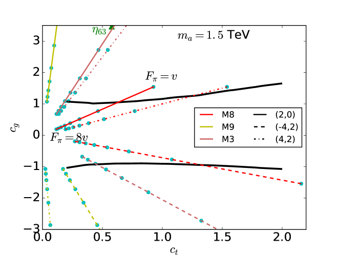
Figure 15: In black thick lines the exclusion limits for the partial-compositeness models considered here are drawn. An integrated luminosity of $L=20\,{\rm fb}^{-1}$ and an uncertainty of $\epsilon_{\rm SYS}=5\%$ are assumed. The model lines refer to models M8 (in red), M9 (yellow) and M3 (brown) introduced in the text. The styles of the lines represent the fermionic charges: $(n_{\psi},n_{\xi})=(2,0)$ (solid line), (-4,2) (dashed) and (4,2) (dot-dashed). Each line scans the values of $F_{\pi}$ from $v$ (most external and largest couplings) to $8v$ (most internal and smallest couplings), the dots represent the values $F_{\pi}=n\,v$, with $n$ an integer between 1 and 8 included.

V.3 Broad scalar color singlet

In this benchmark scenario we assume a CP-even color-singlet scalar that can, apart from top quarks and gluons, also decay into other particles and is thus much broader than the previous scenarios. We choose a total width of 20% of the resonance mass $\Gamma_{\sigma}=20\%\,m_{\sigma}$. The rationale for choosing a larger width is the fact that the scalar tends to decay also to weak bosons. Indeed, we expect a large sensitivity in this decay channel which might be competitive w.r.t. top pair production.

In this scenario the signal is very weak and thus hard to be observed unless the systematic uncertainty is improved to values below 5% or higher values of $c_{g}>3$ are considered. In Fig. 16 on the left we show the line-shape for $m_{\sigma}=900\,{\rm\,\text{GeV}}$, $c_{t}=c_{g}=1$. It can be noticed that the yields are always below 5%. On the right panel we show the $\chi^{2}_{10}=2$ contours in the $(m_{\eta},c_{g})$ parameter space plane for $c_{t}=1$. Varying the assumed systematic uncertainties between $\epsilon_{\rm SYS}=1\%-2\%$ determines the band of the exclusion limit. The integrated luminosities are $L=20\,{\rm fb}^{-1}$ (blue line) and $L=300\,{\rm fb}^{-1}$ (black). Limits are given considering interference (dashed lines) and neglecting it (solid lines). A large interference effect can be noticed, which is in fact larger than the pure signal.

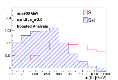
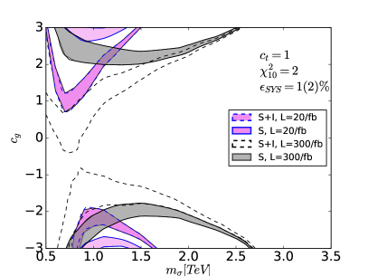
Figure 16: Left: Normalized top-pair mass distributions $r$ for a color-singlet scalar with $c_{g}=c_{t}=1$, $m_{\sigma}=900\,{\rm\,\text{GeV}}$ and $\Gamma_{\sigma}=20\%\,m_{\sigma}$. Right: Exclusion limit ($\chi^{2}=2$) in the $(m_{\sigma},c_{g})$ parameter space and $c_{t}=1$ for such scalar state. The color scheme is the same as in Fig. 11. In both panels the Boosted analysis have been adopted.

VI Conclusion

In this work we have provided a framework to reinterpret the SM $t\bar{t}$ differential cross section measurements in terms of exclusion limits for signatures of NP scalar resonances decaying into $t\bar{t}$. The method relies on the detailed simulation of the SM prediction at particle level with the Sherpa Monte Carlo, the subsequent analysis in the Rivet framework, which can be directly compared with the measured distributions provided by the experimental collaborations, a modeling of the NP scenarios efficient enough to allow a scan over a large range in parameter space, and finally a statistical analysis to determine the excluded regions.

In the simulation of top-pair production we take into account higher-order QCD corrections through matching LO or NLO matrix elements to parton showers and merging partonic processes of varying multiplicity. To validate our simulation we compare to data from the ATLAS collaboration, finding very good agreement. As New Physics contributions we consider CP-even and CP-odd scalar resonances, being either color-singlets or octets. To model the signal we devise an efficient and fast reweighting method allowing to scan large regions of parameter space without the need of full re-simulation and re-analysis for each parameter point. For our simplified model we have derived exclusion limits based on a simple $\chi^{2}$ analysis, that can subsequently be used to set limits on other specific models, and we consider a model of partial compositness as an example. We showed the importance of properly accounting for interference between the New Physics signal and the SM background in setting the exclusion limit, as well as of using a full line-shape analysis which is not necessarily a simple Breit-Wigner shape due to the interference effects.

By confronting SM precision measurements with hypotheses for New Physics models stringent exclusion limits on the parameters of the latter can be obtained, providing complementary sensitivity to direct searches. The methodology laid out here can be readily applied to other observables than the top-pair invariant mass considered here. It relies on a solid understanding of the respective SM expectation and the uncertainties related to the theoretical predictions and the experimental data.

Appendix A Line-shapes samples

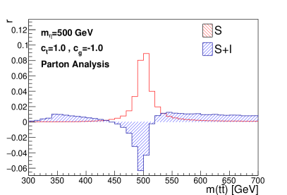
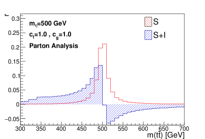
Figure 17: Normalized top-pair mass distributions, $r_{H}=\frac{d\sigma(H)/dm}{d\sigma_{\rm SM}/dm}$ ($H=S,S+I$), for a pseudo-scalar signal ($m_{\eta}=500$ GeV) in the Parton Analysis.

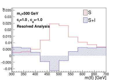
Figure 18: Normalized top-pair mass distributions, $r_{H}=\frac{d\sigma(H)/dm}{d\sigma_{\rm SM}/dm}$ ($H=S,S+I$), for a pseudo-scalar signal ($m_{\eta}=500$ GeV) in the Resolved Analysis.

References

- (1) V. Barger, W.-Y. Keung, and B. Yencho, Azimuthal Correlations in Top Pair Decays and The Effects of New Heavy Scalars, Phys. Rev. D85 (2012) 034016, [arXiv:1112.5173].
- (2) S. Choi and H. S. Lee, Azimuthal decorrelation in production at hadron colliders, Phys. Rev. D87 (2013), no. 3 034012, [arXiv:1207.1484].
- (3) D. Buarque Franzosi and C. Zhang, Probing the top-quark chromomagnetic dipole moment at next-to-leading order in QCD, Phys. Rev. D91 (2015), no. 11 114010, [arXiv:1503.08841].
- (4) C. Zhang, Single Top Production at Next-to-Leading Order in the Standard Model Effective Field Theory, Phys. Rev. Lett. 116 (2016), no. 16 162002, [arXiv:1601.06163].
- (5) C. Englert, L. Moore, K. Nordström, and M. Russell, Giving top quark effective operators a boost, Phys. Lett. B763 (2016) 9–15, [arXiv:1607.04304].
- (6) V. Cirigliano, W. Dekens, J. de Vries, and E. Mereghetti, Constraining the top-Higgs sector of the Standard Model Effective Field Theory, Phys. Rev. D94 (2016), no. 3 034031, [arXiv:1605.04311].
- (7) CDF Collaboration, T. Aaltonen et al., Search for New Color-Octet Vector Particle Decaying to t anti-t in p anti-p Collisions at s**(1/2) = 1.96-TeV, Phys. Lett. B691 (2010) 183–190, [arXiv:0911.3112].
- (8) CMS Collaboration, V. Khachatryan et al., Search for resonant production in proton-proton collisions at 8 TeV, Phys. Rev. D93 (2016), no. 1 012001, [arXiv:1506.03062].
- (9) CMS Collaboration, S. Chatrchyan et al., Searches for new physics using the invariant mass distribution in pp collisions at =8 TeV, Phys. Rev. Lett. 111 (2013), no. 21 211804, [arXiv:1309.2030]. [Erratum: Phys. Rev. Lett.112,no.11,119903(2014)].
- (10) T. Gleisberg, S. Höche, F. Krauss, M. Schönherr, S. Schumann, F. Siegert, and J. Winter, Event generation with SHERPA 1.1, JHEP 02 (2009) 007, [arXiv:0811.4622].
- (11) A. Buckley, J. Butterworth, L. Lönnblad, D. Grellscheid, H. Hoeth, J. Monk, H. Schulz, and F. Siegert, Rivet user manual, Comput. Phys. Commun. 184 (2013) 2803–2819, [arXiv:1003.0694].
- (12) ATLAS Collaboration, G. Aad et al., Measurement of the differential cross-section of highly boosted top quarks as a function of their transverse momentum in = 8 TeV proton-proton collisions using the ATLAS detector, Phys. Rev. D93 (2016), no. 3 032009, [arXiv:1510.03818].
- (13) ATLAS Collaboration, G. Aad et al., Measurements of top-quark pair differential cross-sections in the lepton+jets channel in collisions at TeV using the ATLAS detector, Eur. Phys. J. C76 (2016), no. 10 538, [arXiv:1511.04716].
- (14) J. M. Butterworth, D. Grellscheid, M. Krämer, B. Sarrazin, and D. Yallup, Constraining new physics with collider measurements of Standard Model signatures, JHEP 03 (2017) 078, [arXiv:1606.05296].
- (15) T. Gleisberg, S. Höche, F. Krauss, A. Schälicke, S. Schumann, and J.-C. Winter, SHERPA 1. alpha: A Proof of concept version, JHEP 02 (2004) 056, [hep-ph/0311263].
- (16) S. Schumann and F. Krauss, A Parton shower algorithm based on Catani-Seymour dipole factorisation, JHEP 03 (2008) 038, [arXiv:0709.1027].
- (17) S. Höche, F. Krauss, S. Schumann, and F. Siegert, QCD matrix elements and truncated showers, JHEP 05 (2009) 053, [arXiv:0903.1219].
- (18) S. Höche, F. Krauss, M. Schönherr, and F. Siegert, QCD matrix elements + parton showers: The NLO case, JHEP 04 (2013) 027, [arXiv:1207.5030].
- (19) T. Gleisberg and S. Höche, Comix, a new matrix element generator, JHEP 12 (2008) 039, [arXiv:0808.3674].
- (20) S. Actis, A. Denner, L. Hofer, J.-N. Lang, A. Scharf, and S. Uccirati, RECOLA: REcursive Computation of One-Loop Amplitudes, Comput. Phys. Commun. 214 (2017) 140–173, [arXiv:1605.01090].
- (21) B. Biedermann, S. Bräuer, A. Denner, M. Pellen, S. Schumann, and J. M. Thompson, Automation of NLO QCD and EW corrections with Sherpa and Recola, Eur. Phys. J. C77 (2017) 492, [arXiv:1704.05783].
- (22) A. Denner, S. Dittmaier, and L. Hofer, Collier: a fortran-based Complex One-Loop LIbrary in Extended Regularizations, Comput. Phys. Commun. 212 (2017) 220–238, [arXiv:1604.06792].
- (23) S. Höche, S. Kuttimalai, S. Schumann, and F. Siegert, Beyond Standard Model calculations with Sherpa, Eur. Phys. J. C75 (2015), no. 3 135, [arXiv:1412.6478].
- (24) F. Krauss, D. Napoletano, and S. Schumann, Simulating -associated production of and Higgs bosons with the SHERPA event generator, Phys. Rev. D95 (2017), no. 3 036012, [arXiv:1612.04640].
- (25) J. Alwall, R. Frederix, S. Frixione, V. Hirschi, F. Maltoni, O. Mattelaer, H. S. Shao, T. Stelzer, P. Torrielli, and M. Zaro, The automated computation of tree-level and next-to-leading order differential cross sections, and their matching to parton shower simulations, JHEP 07 (2014) 079, [arXiv:1405.0301].
- (26) T. Sjöstrand, S. Ask, J. R. Christiansen, R. Corke, N. Desai, P. Ilten, S. Mrenna, S. Prestel, C. O. Rasmussen, and P. Z. Skands, An Introduction to PYTHIA 8.2, Comput. Phys. Commun. 191 (2015) 159–177, [arXiv:1410.3012].
- (27) P. Artoisenet, R. Frederix, O. Mattelaer, and R. Rietkerk, Automatic spin-entangled decays of heavy resonances in Monte Carlo simulations, JHEP 03 (2013) 015, [arXiv:1212.3460].
- (28) J. Alwall et al., Comparative study of various algorithms for the merging of parton showers and matrix elements in hadronic collisions, Eur. Phys. J. C53 (2008) 473–500, [arXiv:0706.2569].
- (29) M. Dobbs and J. B. Hansen, The HepMC C++ Monte Carlo event record for High Energy Physics, Comput. Phys. Commun. 134 (2001) 41–46.
- (30) M. Cacciari, G. P. Salam, and G. Soyez, The Anti-k(t) jet clustering algorithm, JHEP 04 (2008) 063, [arXiv:0802.1189].
- (31) M. Cacciari, G. P. Salam, and G. Soyez, The Catchment Area of Jets, JHEP 04 (2008) 005, [arXiv:0802.1188].
- (32) M. Cacciari and G. P. Salam, Pileup subtraction using jet areas, Phys. Lett. B659 (2008) 119–126, [arXiv:0707.1378].
- (33) D. Krohn, J. Thaler, and L.-T. Wang, Jet Trimming, JHEP 02 (2010) 084, [arXiv:0912.1342].
- (34) ATLAS Collaboration, G. Aad et al., Performance of jet substructure techniques for large- jets in proton-proton collisions at = 7 TeV using the ATLAS detector, JHEP 09 (2013) 076, [arXiv:1306.4945].
- (35) J. M. Butterworth, B. E. Cox, and J. R. Forshaw, scattering at the CERN LHC, Phys. Rev. D65 (2002) 096014, [hep-ph/0201098].
- (36) S. Höche, F. Krauss, M. Schönherr, and F. Siegert, NLO matrix elements and truncated showers, JHEP 08 (2011) 123, [arXiv:1009.1127].
- (37) E. Bothmann, M. Schönherr, and S. Schumann, Reweighting QCD matrix-element and parton-shower calculations, Eur. Phys. J. C76 (2016), no. 11 590, [arXiv:1606.08753].
- (38) M. Czakon, D. Heymes, and A. Mitov, Bump hunting in LHC events, Phys. Rev. D94 (2016), no. 11 114033, [arXiv:1608.00765].
- (39) A. V. Manohar and M. B. Wise, Flavor changing neutral currents, an extended scalar sector, and the Higgs production rate at the CERN LHC, Phys. Rev. D74 (2006) 035009, [hep-ph/0606172].
- (40) E. Farhi and L. Susskind, Technicolor, Phys. Rept. 74 (1981) 277.
- (41) A. Belyaev, G. Cacciapaglia, H. Cai, G. Ferretti, T. Flacke, A. Parolini, and H. Serodio, Di-boson signatures as Standard Candles for Partial Compositeness, JHEP 01 (2017) 094, [arXiv:1610.06591].
- (42) G. C. Branco, P. M. Ferreira, L. Lavoura, M. N. Rebelo, M. Sher, and J. P. Silva, Theory and phenomenology of two-Higgs-doublet models, Phys. Rept. 516 (2012) 1–102, [arXiv:1106.0034].
- (43) A. Hayreter and G. Valencia, LHC constraints on color octet scalars, arXiv:1703.04164.
- (44) ATLAS Collaboration, G. Aad et al., Search for new phenomena with photon+jet events in proton-proton collisions at TeV with the ATLAS detector, JHEP 03 (2016) 041, [arXiv:1512.05910].
- (45) ATLAS Collaboration, M. Aaboud et al., Search for new phenomena in high-mass final states with a photon and a jet from collisions at = 13 TeV with the ATLAS detector, arXiv:1709.10440.
- (46) A. Alloul, N. D. Christensen, C. Degrande, C. Duhr, and B. Fuks, FeynRules 2.0 - A complete toolbox for tree-level phenomenology, Comput. Phys. Commun. 185 (2014) 2250–2300, [arXiv:1310.1921].
- (47) C. Degrande, C. Duhr, B. Fuks, D. Grellscheid, O. Mattelaer, et al., UFO - The Universal FeynRules Output, Comput.Phys.Commun. 183 (2012) 1201–1214, [arXiv:1108.2040].
- (48) J. Alwall, M. Herquet, F. Maltoni, O. Mattelaer, and T. Stelzer, MadGraph 5 : Going Beyond, JHEP 1106 (2011) 128, [arXiv:1106.0522].
- (49) M. Czakon, D. Heymes, A. Mitov, D. Pagani, I. Tsinikos, and M. Zaro, Top-pair production at the LHC through NNLO QCD and NLO EW, arXiv:1705.04105.
- (50) K. J. F. Gaemers and F. Hoogeveen, Higgs Production and Decay Into Heavy Flavors With the Gluon Fusion Mechanism, Phys. Lett. B146 (1984) 347.
- (51) D. Dicus, A. Stange, and S. Willenbrock, Higgs decay to top quarks at hadron colliders, Phys. Lett. B333 (1994) 126–131, [hep-ph/9404359].
- (52) R. Frederix and F. Maltoni, Top pair invariant mass distribution: A Window on new physics, JHEP 01 (2009) 047, [arXiv:0712.2355].
- (53) S. Gori, I.-W. Kim, N. R. Shah, and K. M. Zurek, Closing the Wedge: Search Strategies for Extended Higgs Sectors with Heavy Flavor Final States, Phys. Rev. D93 (2016), no. 7 075038, [arXiv:1602.02782].
- (54) S. Jung, J. Song, and Y. W. Yoon, Dip or nothingness of a Higgs resonance from the interference with a complex phase, Phys. Rev. D92 (2015), no. 5 055009, [arXiv:1505.00291].
- (55) A. Djouadi, J. Ellis, and J. Quevillon, Interference effects in the decays of spin-zero resonances into and , JHEP 07 (2016) 105, [arXiv:1605.00542].
- (56) W. Bernreuther, P. Galler, C. Mellein, Z. G. Si, and P. Uwer, Production of heavy Higgs bosons and decay into top quarks at the LHC, Phys. Rev. D93 (2016), no. 3 034032, [arXiv:1511.05584].
- (57) B. Hespel, F. Maltoni, and E. Vryonidou, Signal background interference effects in heavy scalar production and decay to a top-anti-top pair, JHEP 10 (2016) 016, [arXiv:1606.04149].
- (58) D. Buarque Franzosi, E. Vryonidou, and C. Zhang, Scalar production and decay to top quarks including interference effects at NLO in QCD in an EFT approach, JHEP 10 (2017) 096, [arXiv:1707.06760].
- (59) ATLAS Collaboration, M. Aaboud et al., Search for heavy Higgs bosons decaying to a top quark pair in collisions at TeV with the ATLAS detector, arXiv:1707.06025.
- (60) P. Fileviez Perez, R. Gavin, T. McElmurry, and F. Petriello, Grand Unification and Light Color-Octet Scalars at the LHC, Phys. Rev. D78 (2008) 115017, [arXiv:0809.2106].
- (61) I. V. Frolov, M. V. Martynov, and A. D. Smirnov, Resonance contribution of scalar color octet to production at the LHC in the minimal four-color quark–lepton symmetry model, Mod. Phys. Lett. A31 (2016), no. 39 1650224, [arXiv:1610.08409].
- (62) M. Gerbush, T. J. Khoo, D. J. Phalen, A. Pierce, and D. Tucker-Smith, Color-octet scalars at the CERN LHC, Phys. Rev. D77 (2008) 095003, [arXiv:0710.3133].
- (63) C. Kim and T. Mehen, Color Octet Scalar Bound States at the LHC, Phys. Rev. D79 (2009) 035011, [arXiv:0812.0307].
- (64) S. Schumann, A. Renaud, and D. Zerwas, Hadronically decaying color-adjoint scalars at the LHC, JHEP 09 (2011) 074, [arXiv:1108.2957].
- (65) ATLAS Collaboration, M. Aaboud et al., Measurements of top-quark pair differential cross-sections in the lepton+jets channel in collisions at =13 TeV using the ATLAS detector, arXiv:1708.00727.
- (66) CMS Collaboration, S. Chatrchyan et al., Search for resonant production in lepton+jets events in collisions at TeV, JHEP 12 (2012) 015, [arXiv:1209.4397].
- (67) CMS Collaboration, A. M. Sirunyan et al., Search for resonances in highly-boosted lepton+jets and fully hadronic final states in proton-proton collisions at 13 TeV, arXiv:1704.03366.
- (68) ATLAS Collaboration, M. Aaboud et al., Search for new phenomena in dijet events using 37 fb-1 of collision data collected at 13 TeV with the ATLAS detector, Phys. Rev. D96 (2017), no. 5 052004, [arXiv:1703.09127].
- (69) ATLAS Collaboration, M. Aaboud et al., Search for new phenomena in high-mass diphoton final states using 37 fb-1 of proton–proton collisions collected at TeV with the ATLAS detector, Phys. Lett. B775 (2017) 105–125, [arXiv:1707.04147].
- (70) C. Anastasiou, C. Duhr, F. Dulat, E. Furlan, T. Gehrmann, F. Herzog, A. Lazopoulos, and B. Mistlberger, CP-even scalar boson production via gluon fusion at the LHC, arXiv:1605.05761.
- (71) T. Alanne, M. T. Frandsen, and D. Buarque Franzosi, Testing a dynamical origin of Standard Model fermion masses, Phys. Rev. D94 (2016) 071703, [arXiv:1607.01440].