Utilization-Based Scheduling of Flexible Mixed-Criticality Real-Time Tasks

Abstract

Mixed-criticality models are an emerging paradigm for the design of real-time systems because of their significantly improved resource efficiency. However, formal mixed-criticality models have traditionally been characterized by two impractical assumptions: once any high-criticality task overruns, all low-criticality tasks are suspended and all other high-criticality tasks are assumed to exhibit high-criticality behaviors at the same time. In this paper, we propose a more realistic mixed-criticality model, called the flexible mixed-criticality (FMC) model, in which these two issues are addressed in a combined manner. In this new model, only the overrun task itself is assumed to exhibit high-criticality behavior, while other high-criticality tasks remain in the same mode as before. The guaranteed service levels of low-criticality tasks are gracefully degraded with the overruns of high-criticality tasks. We derive a utilization-based technique to analyze the schedulability of this new mixed-criticality model under EDF-VD scheduling. During run time, the proposed test condition serves an important criterion for dynamic service level tuning, by means of which the maximum available execution budget for low-criticality tasks can be directly determined with minimal overhead while guaranteeing mixed-criticality schedulability. Experiments demonstrate the effectiveness of the FMC scheme compared with state-of-the-art techniques.

1 Introduction

A mixed-criticality (MC) system is a system in which tasks with different criticality levels share a computing platform. In MC systems, different degrees of assurance must be provided for tasks with different criticality levels. To improve resource efficiency, MC systems [26] often specify different WCETs for each task at all existing criticality levels, with those at higher criticality levels being more pessimistic. Normally, tasks are scheduled with less pessimistic WCETs for resource efficiency. Only when the less pessimistic WCET is violated, the system switches to the high-criticality mode and only tasks with higher criticality levels are guaranteed to be scheduled with pessimistic WCETs thereafter.

There is a large body of research work on specifying and scheduling mixed-criticality systems (see [8] for a comprehensive review). However, to ensure the safety of high-criticality tasks, the classic MC model [4, 5, 1, 3, 2] applies conservative restrictions to the mode-switching scheme. In the classic MC model, whenever any high-criticality task overruns, all low-criticality tasks are immediately abandoned and all other high-criticality tasks are assumed to exhibit high-criticality behaviors. This mode-switching scheme is not realistic in the following two important respects.

• First, it is pessimistic to immediately abandon all low-criticality tasks, because low-criticality tasks require a certain timing performance as well [17, 25].

• Second, it is pessimistic to bind the mode switches of all high-criticality tasks together for the scenarios where the mode switches of high-criticality tasks are naturally independent [12, 22].

Although there has been some research on solving the first problem, i.e., statically reserving a certain degraded level of service for low-criticality execution [7, 25, 24, 16], to our knowledge, little work has been done to date to address the second problem.

In this paper, we propose a flexible MC model (denoted as FMC) on a uni-processor platform, in which the two aforementioned issues are addressed in a combined manner. In FMC, the mode switches of all high-criticality tasks are independent. A single high-criticality task that violates its low-criticality WCET triggers only itself into high-criticality mode, rather than triggering all high-criticality tasks. All other high-criticality tasks remain at their previous criticality levels and thus do not require to book additional resources at mode-switching points. In this manner, significant resources can be saved compared with the classic MC model [1, 2, 3]. On the other hand, these saved resources can be used by low-criticality tasks to improve their service quality. More importantly, the proposed FMC model adaptively tunes the service level for low-criticality tasks to compensate for the overrun of high-criticality tasks, thereby allowing the system workload to be balanced with minimal service degradation for low-criticality tasks. At each independent mode-switching point, the service level for low-criticality tasks is dynamically updated based on the overruns of high-criticality tasks. By doing so, the quality of service (QoS) for low-criticality tasks can be significantly improved.

Since the service level for low-criticality tasks is dynamically determined during run time, the decision-making procedure should be light-weighted. For this purpose, utilization-based scheduling is more desirable for run-time decision-making because of its simplicity. However, using utilization-based scheduling for our FMC model brings new challenges due to the intrinsic dynamics of this model, such as the service level tuning strategy. In particular, utilization-based schedulability analysis relies on whether the cumulative execution time of low-criticality tasks can be effectively upper bounded. In FMC, the service levels for low-criticality tasks are dynamically tuned at each mode switching point. Therefore, the cumulative execution time of low-criticality tasks strongly depends on when mode switches occur. In general, such information is difficult to explicitly represent prior to real execution, because the independence of the mode switches in FMC results in a large analysis space. It is computationally infeasible to analyze all possibilities. To resolve this challenge, we propose a novel approach based on mathematical induction, which allows the cumulative execution time of low-criticality tasks to be effectively upper bounded.

In this work, we study the schedulability of the proposed FMC model under EDF-VD scheduling. A utilization-based schedulability test condition is derived by integrating the independent triggering scheme and the adaptive service level tuning scheme. A formal proof of the correctness of this new schedulability test condition is presented. Based on this test condition, an EDF-VD-based MC scheduling algorithm, called FMC-EDF-VD, is proposed for the scheduling of an FMC task system. During run time, the optimal service level for low-criticality tasks can be directly determined via this condition with minimum overhead, and mixed-criticality schedulability can be simultaneously guaranteed. In addition, we explore the feasible region of the virtual deadline factor for FMC model. Simulation results show that FMC-EDF-VD provides benefits in supporting low-criticality execution compared with state-of-the-art algorithms.

2 Related Work

Mixed-criticality scheduling is a research field that has received considerable attention in recent years. As stated in [7], much existing research work [1, 2, 3] on MC scheduling makes the pessimistic assumption that all low-criticality tasks are immediately abandoned once the system enters high-criticality mode. Instead of abandoning all low-criticality tasks, some efforts [7, 25, 24, 16, 19] have been made to provide solutions for offering low-criticality tasks a certain degraded service quality when the system is in high-criticality mode. Nevertheless, these studies still use a pessimistic mode-switch triggering scheme in which, whenever one high-criticality task overruns, all other high-criticality tasks are triggered to exhibit high-criticality behavior and book unnecessary resources.

Recent work presented in [12, 22, 15] offers solutions for improving performance for low-criticality tasks by using different mode-switch triggering strategies. Huang et al. [15] proposed an interference constraint graph to specify the execution dependencies between high-criticality and low-criticality tasks. However, this approach still uses high-confidence WCET estimates for all high-criticality tasks when determining system schedulability, and therefore does not address the second problem discussed above. Gu et al. [12] presented a component-based strategy in which the component boundaries offer the isolation necessary to support the execution of low-criticality tasks. Minor overruns can be handled with an internal mode switch by dropping off all low-criticality jobs within a component. More extensive overruns will result in a system-wide external mode switch and the dropping off of all low-criticality jobs. Therefore, the mode switches at the internal and external levels still use pessimistic strategy in which all low-criticality tasks are abandoned once a mode switch occurs at the corresponding level. The two problems mentioned above still exist at both levels. In addition, the system schedulability is tested using a demand bound function (DBF) based approach. The complexity of the schedulability test is exponential in the size of the input [12], resulting in costly computations.

Ren and Phan [22] proposed a partitioned scheduling algorithm based on group-based Pfair-like scheduling [14] for mixed-criticality systems. Within a task group, a single high-criticality task is encapsulated with several low-criticality tasks. The tasks are scheduled via Pfair-like scheduling [14] by breaking them into quantum-length sub-tasks. Sub-tasks that belong to different groups are scheduled on an earliest-pseudo-deadline-first (EPDF) basis. Pfair scheduling is a well-known optimal scheduling method for scheduling periodic real-time tasks on a multiple-resource system. However, Pfair scheduling poses many practical problems [14]. First, the Pfair algorithm incurs very high scheduling overhead because of frequent preemptions caused by the small quantum lengths. Second, the task groups are explicitly required to be well synchronized and to make progress at a steady rate [27]. Therefore, the work presented in [22] strongly relies on the periodic task models. In addition, the system schedulability in [22] is determined by solving a MINLP problem, which in general has NP-hard complexity[11]. Because of this complexity, the scalability problem needs to be carefully considered.

Compared with the existing work [12, 22], the proposed FMC model and its scheduling techniques offer both simplicity and flexibility. In particular, our work differs from these approaches in the following respects. Compared with the Pfair-based scheduling method [22] which relies on periodic task models, our paper derives an EDF-VD-based scheduling scheme for sporadic mixed-criticality task systems, that incorporates an independent mode-switch triggering scheme and an adaptive service level tuning scheme. EDF-VD has shown strong competence in both theoretical and empirical evaluations [4]. Compared with the work presented in [12], our approach uses a more flexible strategy that allows a component/system to abandon low-criticality tasks in accordance with run-time demands. Therefore, both of the problems stated above are addressed in our approach. In contrast to the work of [12, 22], our approach is based on a utilization-based schedulability analysis. The system schedulability can be effectively determined. From the designer’s perspective, our utilization-based approach requires simpler specifications and reasoning compared with the work of [22, 12]. In terms of flexibility, our approach can efficiently allocate execution budgets for low-criticality tasks during runtime in accordance with demands, whereas the approaches presented in [12, 22] require that low-criticality tasks should be executed in accordance with the dependencies between low-criticality and high-criticality tasks that have been determined in off-line.

3 System Models and Background

3.1 FMC implicit-deadline sporadic task model

Task model: We consider an MC system with two different criticality levels, HI and LO. The task set $\gamma$ contains $n$ MC implicit-deadline sporadic tasks which are scheduled on a uni-processor platform. Each task $\tau_{i}$ in $\gamma$ generates an infinite sequence of jobs and can be specified by a tuple $\{T_{i},L_{i},\mathcal{C}_{i}\}$. Here, $T_{i}$ denotes the minimum job-arrival intervals. $L_{i}\in\{LO,HI\}$ denotes the criticality level of a task. Each task is either a low-criticality task or high-criticality task. $\gamma_{LO}$ and $\gamma_{HI}$ (where $\gamma=\gamma_{LO}\cup\gamma_{HI}$) denote low-criticality task set and high-criticality task set, respectively. $\mathcal{C}_{i}\in\{C_{i}^{LO},C_{i}^{HI}\}$ is the list of WCETs, where $C_{i}^{LO}$ and $C_{i}^{HI}$ denote the low-criticality and high-criticality WCETs, respectively.

For high-criticality tasks, the WCETs satisfy $C_{i}^{LO}<C_{i}^{HI}$. For low-criticality tasks, their execution budget is dynamically determined in FMC based on the overruns of high-criticality tasks. To characterize the execution behavior of low-criticality tasks in high-criticality mode, we now introduce the concept of the service level on each mode-switching point, which specifies the guaranteed service quality after the mode switch.

Service level: Instead of completely discarding all low-criticality tasks, Burns and Baruah in [7] proposed a more practical MC task model in which low-criticality tasks are allowed to statically reserve resources for their execution at a degraded service level in high-criticality mode (i.e., a reduced execution budget). By contrast, in FMC, the execution budget is dynamically determined based on the run-time overruns rather than statically reserved as in [7]. To model this dynamic behavior, the service level concept defined in [7] should be extended to apply to independent mode switches. Therefore, we define the service level $z_{i}^{k}$ when the system has undergone $k$ mode switches.

Definition 1

(Service level $z_{i}^{k}$ when $k$ mode switches have occurred). If low-criticality task $\tau_{i}$ is executed at service level $z_{i}^{k}$ when the system has undergone $k$ mode switches, up to $z_{i}^{k}\cdot{}C_{i}^{LO}$ time units can be used for the execution of $\tau_{i}$ in one period $T_{i}$. When $\tau_{i}$ runs in low-criticality mode, we say $\tau_{i}$ is executed at service level $z_{i}^{0}$, where $z_{i}^{0}=1$.

The service level definition given above is compliant with the concept of the imprecise computation model developed by Lin et al.[18] to deal with time-constrained iterative calculations. Imprecise computation model is partly motivated by the observation that many real-time computations are iterative in nature, solving a numeric problem by successive approximations. Terminating an iteration early can return useful imprecise results. With this motivation in mind, the imprecise computation model can be used in a natural way to enhance graceful degradation [20]. The practicality of imprecise computation model has been deeply investigated and verified in [9]. Imprecise computation model provides an approximate but timely result, which may be acceptable in many application areas. Examples of such applications are optimal control [6], multimedia applications [21], image and speech processing [10], and fault-tolerant scheduling problems [13]. In FMC, when an overrun occurs, low-criticality tasks will be terminated before completion and sacrifice the quality of the produced results to ensure their timing correctness.

Assumptions: For the remainder of the manuscript, we make the following assumptions: (1) Regarding the compensation for the $k^{\textit{th}}$ overrun of a high-criticality task, we assume that $z_{i}^{k}\leq{z_{i}^{k-1}}$. After the $k^{\textit{th}}$ mode-switching point, the allowed execution time budget in one period should thus be reduced from $z_{i}^{k-1}\cdot{c_{i}^{LO}}$ to $z_{i}^{k}\cdot{c_{i}^{LO}}$. (2) According to [4], if $u_{LO}^{LO}+u_{HI}^{HI}\leq{1}$, then all tasks can be perfectly scheduled by regular EDF under the worst-case reservation strategy. Therefore, we here consider meaningful cases in which $u_{LO}^{LO}+u_{HI}^{HI}>{1}$.

Utilization: Low and high utilization for a task $\tau_{i}$ are defined as $u_{i}^{LO}=\frac{c_{i}^{LO}}{T_{i}}$ and $u_{i}^{HI}=\frac{c_{i}^{HI}}{T_{i}}$, respectively. The system-level utilization for task set $\gamma$ are defined as $u_{LO}^{LO}=\sum_{\tau_{i}\in{\gamma_{LO}}}u_{i}^{LO}$, $u_{HI}^{LO}=\sum_{\tau_{i}\in{\gamma_{HI}}}u_{i}^{LO}$, and $u_{HI}^{HI}=\sum_{\tau_{i}\in{\gamma_{HI}}}u_{i}^{HI}$. The system utilization of low-criticality tasks after $k^{\textit{th}}$ mode-switching point can be defined as $u_{LO}^{k}=\sum_{\tau_{i}\in{\gamma_{LO}}}z_{i}^{k}\cdot{}u_{i}^{LO}$. To guarantee the execution of the mandatory portions of low-criticality tasks, the mandatory utilization can be defined as $u_{LO}^{man}=\sum_{\tau_{i}\in{\gamma_{LO}}}z_{i}^{man}\cdot{}u_{i}^{LO}$, where $z_{i}^{man}$ is the mandatory service level for task $\tau_{i}$ as specified by the users.

3.2 Execution semantics of the FMC model

The main differences between our FMC execution model and the classic MC execution model lie in the independent mode-switch triggering scheme for high-criticality tasks and the dynamic service tuning of low-criticality tasks. In contrast to the classic MC model, the FMC model allows an independent triggering scheme in which the overrun of one high-criticality task triggers only itself into high-criticality mode. Consequently, the high-criticality mode of the system in FMC depends on the number of high-criticality tasks that have overrun. Therefore, we introduce the following definition:

Definition 2

($k$-level high-criticality mode). At a given instant of time, if $k$ high-criticality tasks have entered high-criticality mode, then the system is in $k$-level high-criticality mode. For low-criticality mode, we say that the system is in $0$-level high-criticality mode.

Based on Def. 2, the execution semantics of the FMC model is illustrated in Fig. 1. Initially, the system is in low-criticality mode (i.e., $0$-level high-criticality mode). Then, the overruns of high-criticality tasks trigger the system to proceed through the high-criticality modes one by one until the condition for transitioning back is satisfied. According to Fig. 1, the execution semantics can be summarized as follows:

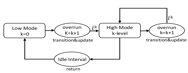
Figure 1: Execution semantics of the FMC model.

• Low-criticality mode: All tasks in $\gamma$ start in $0$-level high-criticality mode (i.e., low-criticality mode). As long as no high-criticality task violates its $C_{i}^{LO}$, the system remains in $0$-level high-criticality mode. In this mode, all tasks are scheduled with $C_{i}^{LO}$.

• Transition: When one job of a high-criticality task that is being executed in low-criticality mode overruns its $C_{i}^{LO}$, this high-criticality task immediately switches into high-criticality mode. However, the overrun of this task does not trigger other high-criticality tasks to enter high-criticality mode. All other high-criticality tasks still remain in the same mode as before. Correspondingly, the system transitions to a higher-level high-criticality mode.

• Updates: At the $k^{\textit{th}}$ transition point (corresponding to time instant $\hat{t}^{k}$ in Fig. 1), a new service level $z_{i}^{k}$ is determined and updated to provide degraded service for low-criticality tasks $\tau_{i}$ to balance the resource demand caused by the overrun of the high-criticality task. At this time, if any low-criticality jobs have completed more than $z_{i}^{k}\cdot{c_{i}^{LO}}$ time units of execution (i.e., have used up the updated execution budget for the current period), those jobs will be suspended immediately and wait for the budget to be renewed in the next period. Otherwise, low-criticality jobs can continue to use the remaining time budget for their execution.

• Return to low-criticality mode: When the system detects an idle interval [7, 23], the system will transition back into low-criticality mode.

3.3 EDF-VD scheduling

EDF-VD [4, 5] is a scheduling algorithm for implementing classic preemptive EDF scheduling in MC systems. The main concept of EDF-VD is to artificially reduce the (virtual) deadlines of high-criticality tasks when the system is in low-criticality mode. These virtual deadlines can be used to cause high-criticality tasks to finish earlier to ensure that the system can reserve a sufficient execution budget for the high-criticality tasks to meet their actual deadlines after the system switches into high-criticality mode. In this paper, we study the schedulability under EDF-VD scheduling for the proposed FMC model.

4 FMC-EDF-VD scheduling algorithm

In this section, we provide an overview of the proposed EDF-VD-based scheduling algorithm for our FMC model, called FMC-EDF-VD. The proposed scheduling algorithm consists of an off-line step and a run-time step. We implement the off-line step prior to run time to select a feasible virtual deadline factor $x$ for tightening the deadlines of high-criticality tasks. During run time, the service levels $z_{i}^{k}$ for low-criticality tasks are dynamically tuned based on the overrun of high-criticality tasks. Here, we present the operation flow of FMC-EDF-VD.

Off-line step: In accordance with Thm. 1, we first determine $x$ as $\frac{u_{HI}^{LO}}{1-u_{LO}^{LO}}$. Then, to guarantee the schedulability of FMC-EDF-VD, the determined $x$ value should be validated by testing condition Eqn. (24) in Thm. 5. Note that if condition Eqn. (24) is not satisfied, then it is reported that the specified task set cannot be scheduled using FMC-EDF-VD.

Run-time step: The run-time behavior follows the execution semantics presented in Section 3.2. In low-criticality mode, all high-criticality tasks are scheduled with their virtual deadlines. At each mode-switching point, the following two procedures are triggered:

• Reset the deadline of overrun high-criticality task from its virtual deadline to the actual deadline. The deadline settings of other high-criticality tasks remain the same as before.

• Update the service levels for low-criticality tasks in accordance with Thm. 2.

Note that various run-time tuning strategies can be specified by the user as long as the condition in Thm. 2 is satisfied. For the purpose of demonstration, a uniform tuning strategy and a dropping-off strategy are discussed in this paper. Complete descriptions of these strategies are provided in Section 6.

Table I: Example task set

	$L_{i}$	$T_{i}$	$C_{i}^{LO}$	$C_{i}^{HI}$
$\tau_{1},\tau_{2},\tau_{3},\tau_{4}$	HI	$40$	$3$	$8$
$\tau_{5}$	LO	$200$	$30$
$\tau_{6}$	LO	$300$	$75$

4.1 Motivational example

In this section, we present a motivation example to show how the global triggering scheme in FMC-EDF-VD can efficiently support low-criticality task execution. The uniform tuning strategy (see Thm. 6), in which all low-criticality tasks share the same service level setting $z^{k}$ during run time (i.e., $\forall\tau_{i}\in{}\gamma_{LO}$, $z_{i}^{k}=z^{k}$), is adopted for this demonstration.

Example 1

For clarity of presentation, we consider a task set that contains four identical high-criticality tasks and two low-criticality tasks, as listed in Tab. I. We specify $u_{LO}^{man}=0$ for demonstration. From Tab. I, one can derive $u_{LO}^{LO}=\frac{2}{5}$, $u_{HI}^{LO}=\frac{3}{10}$, and $u_{HI}^{HI}=\frac{4}{5}$.

According to Thm. 6, we can compute the uniform service levels $z^{k}$ for all possible mode-switching scenarios. The results are listed in Tab. II.

Table II: Low-criticality service levels

Number of Overrun $k$	$1$	$2$	$3$	$4$
Utilization $u_{LO}^{k}$	0.3	0.2	0.1	0
Service Level $z^{k}$	0.75	0.5	0.25	0
Execution Budget of $\tau_{5}$	22.5	15	7.5	0
Execution Budget of $\tau_{6}$	56.25	37.5	18.75	0

As shown in Tab. II, FMC-EDF-VD can efficiently support low-criticality task execution by dynamically tuning the low-criticality execution budget based on overrun demand. When only one high-criticality task overruns, low-criticality task $\tau_{5}$ and $\tau_{6}$ can use up to 22.5 and 56.25 time units per period for execution. In this case, low-criticality tasks can maintain 75% execution. Only when all high-criticality tasks overrun their $C_{i}^{L}$, low-criticality tasks are all dropped. For comparison, the global triggering strategy used in [7, 19] are always required to drop all low-criticality tasks regardless of how many overruns occur during run time because of the overapproximation of the overrun workload. From a probabilistic perspective, the likelihood that all high-criticality tasks will exhibit high-criticality behavior is very low in practice. Therefore, in a typical case, only a few high-criticality tasks will overrun their $C_{i}^{L}$ during a busy interval. In most cases, FMC-EDF-VD will only need to schedule resources for a portion of high-criticality tasks based on their overrun demands and can maintain the service level for low-criticality task execution to the greatest possible extent. In this sense, FMC-EDF-VD can provide better and more graceful service degradation.

5 Schedulability Test Condition

In this section, we present a utilization-based schedulability test condition for the FMC-EDF-VD scheduling algorithm. We start by ensuring the schedulability of the system when it is operating in low-criticality mode (Thm. 1). Then, we discuss how to derive a sufficient condition to ensure the schedulability of the algorithm after $k$ mode switches (Thm. 2). Based on several sophisticated new techniques, the correctness of this new schedulability test condition can be proven and the formal proof is provided in Section 5.3. Finally, we derive the region of $x$ that can guarantee the feasibility of the proposed scheduling algorithm.

5.1 Low-criticality mode

In low-criticality mode, the system behaviors in FMC are exactly the same as in EDF-VD [4]. Therefore, we can use the following theorem presented in [4] to ensure the schedulability of tasks in low-criticality mode.

Theorem 1

The following condition is sufficient to ensure that EDF-VD can successfully schedule all tasks in low-criticality mode:

$$u_{LO}^{LO}+\frac{u_{HI}^{LO}}{x}\leq{1}$$ (1)

5.2 High-criticality mode after $k$ mode switches

In this section, we analyze the schedulability of the FMC-EDF-VD algorithm during the transition phase. With this analysis, we provide the answer to the question of how much execution budget can be reserved for low-criticality tasks while ensuring a schedulable system for mode transitions. Without loss of generality, we consider a general transition case in which the system transitions from $(k-1)$-level high-criticality mode to $k$-level high-criticality mode. Here, we first introduce the derived schedulability test condition in Thm. 2. Then, the formal proof of the correctness of this schedulability test condition is provided in Section 5.3. Recall that $u_{LO}^{k}$ denotes the utilization of low-criticality tasks for the $k^{\textit{th}}$ mode-switching point and is defined as $u_{LO}^{k}=\sum_{\tau_{i}\in{\gamma_{LO}}}z_{i}^{k}\cdot{}u_{i}^{LO}$.

Theorem 2

The system is in $(k-1)$-level high-criticality mode. For the $k^{\textit{th}}$ mode-switching point $\hat{t}^{k}$, when high-criticality task $\tau_{\hat{t}^{k}}$ overruns, the system is schedulable at $\hat{t}^{k}$ if the following conditions are satisfied:

$$u_{LO}^{k} \leq{}u_{LO}^{k-1}+\frac{\frac{u_{\hat{t}^{k}}^{LO}}{u_{HI}^{LO}}(1-u_{LO}^{LO})-u_{\hat{t}^{k}}^{HI}}{(1-x)}$$ (2)

$$z_{i}^{k} \leq{}z_{i}^{k-1}\ \ (\forall\tau_{i}\in\gamma_{LO})$$ (3)

where $u_{\hat{t}^{k}}^{LO}$ and $u_{\hat{t}^{k}}^{HI}$ denote low and high utilization, respectively, for the high-criticality task $\tau_{\hat{t}^{k}}$ that undergoes a mode switch at $\hat{t}^{k}$.

In Thm. 2, we present a general utilization-based schedulability test condition for the FMC model. Now, let us take a closer look at the conditions specified in Thm. 2. We observe the following interesting properties of FMC-EDF-VD:

• In Thm. 2, the desired utilization balance between low-criticality and high-criticality tasks is achieved. As constrained by Eqn. (3), the utilization of low-criticality tasks should be further reduced when a new overrun occurs. As shown in Eqn. (2), the utilization reduction $u_{LO}^{k}-u_{LO}^{k-1}$ is bounded by $\frac{\frac{u_{\hat{t}^{k}}^{LO}}{u_{HI}^{LO}}(1-u_{LO}^{LO})-u_{\hat{t}^{k}}^{HI}}{(1-x)}$ for utilization balance.

• Another important observation is that the bound on the utilization reduction is determined only by the overrun of high-criticality task $\tau_{\hat{t}^{k}}$ (as shown in Eqn. (2)). This means that the effects of the overruns on utilization reduction are independent. Moreover, the occurrence sequence of high-criticality task overruns has no impact on the utilization reduction.

• Thm. 2 also provides us with a generic metric for managing the resources of low-criticality tasks when each independent mode switch occurs. In general, various run-time tuning strategies can be applied during the transition phase, as long as the conditions in Thm. 2 are satisfied.

5.3 The proof of correctness

We now prove the correctness of the schedulability test condition presented in Thm. 2. We start with the proof by introducing some important concepts. Then, we propose a key technique to obtain the bound of the cumulative execution time for low-criticality and high-criticality tasks (Lem. 1, Lem. 2, and Lem. 3). Based on these derived bounds, the utilization-based test condition can be derived.

5.3.1 Challenges

Incorporating the FMC model into a utilization-based EDF-VD scheduling analysis introduces several new challenges. The independent triggering scheme and the adaptive service level tuning scheme in the FMC model allow flexible system behaviors. However, this flexibility also makes the system behavior more complex and more difficult to analyze. In particular, it is difficult to effectively determine an upper bound on the cumulative execution time for low-criticality tasks. In the FMC model, the service levels for low-criticality tasks are dynamically tuned at each mode-switching point. Therefore, the cumulative execution time of low-criticality tasks strongly depends on when each mode switch occurs. However, this information is difficult to explicitly represent prior to real execution because the independence of the mode switches in the FMC model results in a large analysis space. This makes it computationally infeasible to analyze all possibilities. Moreover, apart from the timing information of multiple mode switches, the derivation of the cumulative execution time also depends on the service tuning decisions made at previous mode switches. Determining how to extract static information (i.e., utilization) to formulate a feasible sufficient condition from these variables is another challenging task.

5.3.2 Concepts and notation

Before diving into the detailed proofs, we introduce some commonly used concepts and notation that will be used throughout the proofs. To derive a sufficient test, suppose that there is a time interval $[0,t_{f}]$ such that the system undergoes the $k^{\textit{th}}$ mode switch and the first deadline miss occurs at $t_{f}$. Let $J$ be the minimal set of jobs released from the MC task set $\gamma$ for which a deadline is missed. This minimality means that if any job is removed from $J$, the remainder of $J$ will be schedulable. Here, we introduce some notation for later use. $\hat{t}^{k}$ denotes the time instant of the $k^{\textit{th}}$ mode switch caused by high-criticality task $\tau_{\hat{t}^{k}}$. The absolute release time and deadline of the job of $\tau_{\hat{t}^{k}}$ that overruns at $\hat{t}^{k}$ are denoted by $a_{\hat{t}^{k}}$ and $d_{\hat{t}^{k}}$, respectively. $\eta_{i}^{k}(t_{1},t_{2})$ denotes the cumulative execution time of task $\tau_{i}$ when the system is operating in $k$-level high-criticality mode during the interval $(t_{1},t_{2}]$. Next, we define a special type of job for low-criticality tasks, called a carry-over job, and introduce several important propositions that will be useful for our later proofs.

Definition 3

A job of low-criticality task $\tau_{i}$ is called a $k$-carry-over job if the $k^{\text{th}}$ mode switch occurs in the interval $[a_{i}^{k},d_{i}^{k}]$, where $a_{i}^{k}$ and $d_{i}^{k}$ are the absolute release time and deadline of this job, respectively.

Fig. 2 shows how a $k$-carry-over job is executed during the interval $[a_{i}^{k},d_{i}^{k}]$. The black box represents the cumulative execution time $\eta_{i}^{k}(a_{i}^{k},\hat{t}^{k})$ of the $k$-carry-over job before the $k^{\text{th}}$ mode-switching point $\hat{t}^{k}$.

Figure 2: The execution scenario for a $k$-carry-over job.

Proposition 1

(From [4, 5]) All jobs executed in $[\hat{t}^{k},t_{f}]$ have a deadline $\leq{}t_{f}$.

Proposition 2

The $k^{\textit{th}}$ mode-switching point $\hat{t}^{k}$ satisfies $\hat{t}^{k}\leq a_{\hat{t}^{k}}+x\cdot{(t_{f}-a_{\hat{t}^{k}})}$.

Proof:

Since a high-criticality job of $\tau_{\hat{t}^{k}}$ triggers the $k^{\textit{th}}$ mode switch at $\hat{t}^{k}$, its virtual deadline ${a_{\hat{t}^{k}}+x\cdot{(d_{\hat{t}^{k}}-a_{\hat{t}^{k}})}}$ must be greater than $\hat{t}^{k}$. Otherwise, the high-criticality job would have completed its execution before the time instant of the switch. ∎

Proposition 3

For a $k$-carry-over job of low-criticality task $\tau_{i}$, if $\eta_{i}^{k}(a_{i}^{k},\hat{t}^{k})\neq{0}$, then the following holds: $d_{i}^{k}\leq a_{\hat{t}^{k}}+x\cdot{(t_{f}-a_{\hat{t}^{k}})}$.

Proof:

There are two cases to consider: $a_{i}^{k}\geq a_{\hat{t}^{k}}$ and $a_{i}^{k}<a_{\hat{t}^{k}}$.

Case 1 ($a_{i}^{k}\geq a_{\hat{t}^{k}}$): In this case, for the $k$-carry-over job to be executed after $a_{\hat{t}^{k}}$, the $k$-carry-over job should have a deadline no later than the virtual deadline $a_{\hat{t}^{k}}+x(d_{\hat{t}^{k}}-a_{\hat{t}^{k}})$ of the high-criticality job that triggered the $k^{\text{th}}$ mode switch. As a result, because $d_{\hat{t}^{k}}\leq t_{f}$, we have $d_{i}^{k}\leq(a_{\hat{t}^{k}}+x\cdot{(t_{f}-a_{\hat{t}^{k}})})$.

Case 2 ($a_{i}^{k}<a_{\hat{t}^{k}}$): We prove the correctness of this case by contradiction. Suppose that the $k$-carry-over job of low-criticality task $\tau_{i}$, with its deadline of $d_{i}^{k}>(a_{\hat{t}^{k}}+x\cdot{(t_{f}-a_{\hat{t}^{k}})})$, were to be executed before $a_{\hat{t}^{k}}$. Let $t^{*}$ denote the latest time instant at which this $k$-carry-over job is executed before $a_{\hat{t}^{k}}$. At time instant $\hat{t}^{k}$, all previous $(k-1)$ mode switches are known to the system. At $t^{*}$, we know that there should be no pending job with a deadline of $\leq(a_{\hat{t}^{k}}+x\cdot{(t_{f}-a_{\hat{t}^{k}})})$. This means that jobs that are released at or after $t^{*}$ will also suffer a deadline miss at $t_{f}$, which contradicts the minimality of $J$. Therefore, $d_{i}^{k}\leq({a_{\hat{t}^{k}}+x\cdot{(t_{f}-a_{\hat{t}^{k}})}})$. ∎

Using the propositions and notation presented above, we now derive an upper bound on the cumulative execution time $\eta_{i}^{k}(0,t_{f})$ for low-criticality tasks (Lem. 1) and high-criticality tasks (Lem. 2 and Lem. 3).

5.3.3 Bound for low-criticality tasks

As discussed above, it is difficult to derive an upper bound on the cumulative execution time of low-criticality tasks during the interval $[0,t_{f}]$ because of the large analysis space. In this section, we propose a novel derivation strategy to resolve this challenge. The overall derivation strategy is based on the specified derivation protocol (Rule 1-Rule 4) and mathematical induction. The purpose of the derivation protocol is to specify unified intermediate upper bounds for different execution scenarios. The advantage of introducing these intermediate upper bounds is that we can virtually hide the influence of the previous $k-1$ mode switches. For instance, in Rule 1 (see Eqn. (5.3.3)), the influence of the previous $k-1$ mode switches is hidden in the term $\sup\{\eta_{i}^{k}(0,d_{i}^{l})\}$. In this way, the $k^{\textit{th}}$ mode switch and the previous $k-1$ mode switches are decorrelated.

Throughout the remainder of this section, we will use $\sup{\{\eta_{i}^{k}(t_{1},t_{2})\}}$ to denote the intermediate upper bounds on $\eta_{i}^{k}(t_{1},t_{2})$ for different execution scenarios, which represent the upper bounds under specific conditions. Let $\hat{t}^{k-j}$ ($j>0$) denote the last mode-switching point before $a_{i}^{k}$ (as shown in Fig. 2). $z_{i}^{k-j}$ denotes the updated service level at $\hat{t}^{k-j}$. $d_{i}^{l}$ denotes the absolute deadline for the last job of $\tau_{i}$ during $[0,t_{f}]$. Now, we present the rules for deriving $\sup\{\eta_{i}^{k}(0,t_{f})\}$ and $\sup\{\eta_{i}^{k}(a_{i}^{k},d_{i}^{k})\}$, as summarized in Eqn. (5.3.3) and Eqn. (5.3.3).

$$\sup\{\eta_{i}^{k}(0,t_{f})\}$$

$$= \begin{cases}\sup\{\eta_{i}^{k}(0,d_{i}^{l})\}+(t_{f}-\hat{t}^{k})\cdot{}z_{i}^{k}\cdot{}u_{i}^{LO}&\text{$d_{i}^{l}<\hat{t}^{k}$ ({Rule\leavevmode\nobreak\ \ref{rule:1}})}\\ \sup\{\eta_{i}^{k}(0,d_{i}^{k})\}+(t_{f}-d_{i}^{k})\cdot{}z_{i}^{k}\cdot{}u_{i}^{LO}&\text{Otherwise ({Rule\leavevmode\nobreak\ \ref{rule:2}})}\\ \end{cases}$$ (4)

$$\sup\{\eta_{i}^{k}(a_{i}^{k},d_{i}^{k})\}$$

$$= \begin{cases}{(d_{i}^{k}-a_{i}^{k})\cdot{z_{i}^{k-j}}\cdot{u_{i}^{LO}}}&\text{$\eta_{i}^{k}(a_{i}^{k},\hat{t}^{k})\neq{0}$ ({Rule\leavevmode\nobreak\ \ref{rule:3}})}\\ {(d_{i}^{k}-a_{i}^{k})\cdot{z_{i}^{k}}\cdot{u_{i}^{LO}}}&\text{Otherwise ({Rule\leavevmode\nobreak\ \ref{rule:4}})}\end{cases}$$ (5)

The detailed description and proof are presented in Appendix A. In Rule 1-Rule 4, one may notice that there are several different execution scenarios in which only one mode switch is considered. When $n$ mode switches are allowed, the combination space for all execution scenarios will increase exponentially with $n$. In general, it is very difficult to derive a bound on the cumulative execution time for low-criticality tasks because of this large combination space. To solve this problem, we analyze the difference between $\sup\{\eta_{i}^{k}(0,t_{f})\}$ and $\sup\{\eta_{i}^{k-1}(0,t_{f})\}$ and find that this difference can be uniformly bounded by a difference term $\psi_{i}^{k}$ (see Lem. 1). This finding is formally proven in Lem. 1 through mathematical induction. Before the proof, we first present a fact that will be useful for later interpretation.

Fact 1

For the $k^{\textit{th}}$ mode-switching point $\hat{t}^{k}$, at time instant $t_{0}$ such that $t_{0}\leq{\hat{t}^{k}}$, $\eta_{i}^{k}(0,t_{0})=\eta_{i}^{k-1}(0,t_{0})$.

Proof:

The $k^{\textit{th}}$ mode switch can only begin to affect low-criticality task execution after the corresponding mode-switching point $\hat{t}^{k}$. Before $\hat{t}^{k}$, the $k^{\textit{th}}$ mode switch has no impact. Thus, we have $\eta_{i}^{k}(0,t_{0})=\eta_{i}^{k-1}(0,t_{0})$. ∎

Lemma 1

For all $k\geq{1}$, the cumulative execution time $\eta_{i}^{k}(0,t_{f})$ can be upper bounded by

$$t_{f}\cdot{u_{i}^{LO}}+\sum_{j=1}^{k}\psi_{i}^{j}$$ (6)

where the difference term $\psi_{i}^{j}$ is defined as $(t_{f}-a_{\hat{t}^{j}})(1-x)(z_{i}^{j}-z_{i}^{j-1})u_{i}^{LO}$.

Proof:

Instead of proving the original statement, we will prove an alternative statement $P(k)$, which is defined as follows:

The intermediate upper bounds $\sup\{\eta_{i}^{k}(0,t_{f})\}$ under different execution scenarios can be uniformly upper bounded by Eqn. (6).

Since $\eta_{i}^{k}(0,t_{f})\leq{}\sup\{\eta_{i}^{k}(0,t_{f})\}$, the original statement will be proven correct if the statement $P(k)$ is proven to be correct. Now, we will prove that the statement $P(k)$ is correct for all possible integers $k$ based on mathematical induction. Recall that $d_{i}^{l}$ is the absolute deadline for the last job of $\tau_{i}$ during $[0,t_{f}]$.

Step 1 (base case): We will prove that $P(1)$ is correct for $k=1$.

Proof:

We consider two cases, one in which a carry-over job does not exist at the first mode-switching point $\hat{t}^{1}$ (i.e., $d_{i}^{l}<\hat{t}^{1}$) and one in which such a job does exist (i.e., $d_{i}^{l}\geq{}\hat{t}^{1}$).

Case 1 ($\mathbf{d_{i}^{l}<\hat{t}^{1}}$): According to Rule 1 and Prop. 2, we have the following:

$$\sup\{\eta_{i}^{1}(0,t_{f})\}$$

$$=\sup\{\eta_{i}^{1}(0,d_{i}^{l})\}+(t_{f}-\hat{t}^{1})\cdot{}z_{i}^{1}\cdot{}u_{i}^{LO}$$

$$=d_{i}^{l}\cdot{}u_{i}^{LO}+(t_{f}-\hat{t}^{1})\cdot{}z_{i}^{1}\cdot{}u_{i}^{LO}$$

$$since\ \ d_{i}^{l}<\hat{t}^{1}\leq{}a_{\hat{t}^{1}}+x\cdot{(t_{f}-a_{\hat{t}^{1}})}$$

$$<{}t_{f}\cdot{}z_{i}^{1}\cdot{}u_{i}^{LO}+\hat{t}^{1}\cdot{}u_{i}^{LO}\cdot{}(1-z_{i}^{1})\ \ \ \ \ (replace\ \ d_{i}^{l}\ \ with\ \ \hat{t}^{1})$$

$$\leq{}t_{f}\cdot{}u_{i}^{LO}+\underbrace{(t_{f}-a_{\hat{t}^{1}})(1-x)(z_{i}^{1}-1)u_{i}^{LO}}_{difference\;term\;\psi_{i}^{1}}\ \ \ (replace\ \ \hat{t}^{1})$$

Case 2 ($\mathbf{d_{i}^{l}\geq{}\hat{t}^{1}}$): In this case, we consider the two following execution scenarios.

S1 ($\mathbf{\eta_{i}^{1}(a_{i}^{1},\hat{t}^{1})\neq{0}})$: According to Rule 2, Rule 3, and Prop. 3, we have the following:

$$\sup\{\eta_{i}^{1}(0,t_{f})\}$$

$$= \sup\{\eta_{i}^{1}(0,a_{i}^{1})\}+\sup\{\eta_{i}^{1}(a_{i}^{1},d_{i}^{1})\}+(t_{f}-d_{i}^{1}){z_{i}^{1}}{u_{i}^{LO}}$$

$$= a_{i}^{1}{u_{i}^{LO}}+(d_{i}^{1}-a_{i}^{1}){u_{i}^{LO}}+(t_{f}-d_{i}^{1}){z_{i}^{1}}{u_{i}^{LO}}$$

$$= t_{f}\cdot{}u_{i}^{LO}+(t_{f}-d_{i}^{1})(z_{i}^{1}-1)u_{i}^{LO}$$

$$since\ d_{i}^{1}\leq{a_{\hat{t}^{1}}+x\cdot{(t_{f}-a_{\hat{t}^{1}})}}$$

$$\leq{} t_{f}\cdot{}u_{i}^{LO}+\underbrace{(t_{f}-a_{\hat{t}^{1}})(1-x)(z_{i}^{1}-1)u_{i}^{LO}}_{difference\;term\;\psi_{i}^{1}}\ \ \ (replace\ \ d_{i}^{1})$$

S2 ($\mathbf{\eta_{i}^{1}(a_{i}^{1},\hat{t}^{1})={0}}$): According to Rule 2, Rule 4, and Prop. 2, we have the following:

$$\sup\{\eta_{i}^{1}(0,t_{f})\}$$

$$= \sup\{\eta_{i}^{1}(0,a_{i}^{1})\}+\sup\{\eta_{i}^{1}(a_{i}^{1},d_{i}^{1})\}+(t_{f}-d_{i}^{1}){z_{i}^{1}}{u_{i}^{LO}}$$

$$= a_{i}^{1}{u_{i}^{LO}}+(d_{i}^{1}-a_{i}^{1})z_{i}^{1}{u_{i}^{LO}}+(t_{f}-d_{i}^{1}){z_{i}^{1}}{u_{i}^{LO}}$$

$$= t_{f}\cdot{}u_{i}^{LO}+(t_{f}-a_{i}^{1})(z_{i}^{1}-1)u_{i}^{LO}$$

$$since\ a_{i}^{1}<\hat{t}^{1}\leq{a_{\hat{t}^{1}}+x\cdot{(t_{f}-a_{\hat{t}^{1}})}}$$

$$\leq{} t_{f}\cdot{}u_{i}^{LO}+\underbrace{(t_{f}-a_{\hat{t}^{1}})(1-x)(z_{i}^{1}-1)u_{i}^{LO}}_{difference\;term\;\psi_{i}^{1}}\ \ \ (replace\ \ a_{i}^{1})$$

Therefore, $P(1)$ is correct for $k=1$. ∎

Step 2 (induction hypothesis): Assume that $P(k_{0}-1)$ is correct for some possible integers $k_{0}-1$.

Step 3 (induction): We now prove that $P(k_{0})$ is correct by the induction hypothesis.

Proof:

Since $\hat{t}^{k_{0}-1}\leq{}\hat{t}^{k_{0}}$, we need to consider the following three cases.

Case 1 ($\mathbf{d_{i}^{l}<\hat{t}^{k_{0}-1}\leq{}\hat{t}^{k_{0}}}$): In this case, neither a $(k_{0}-1)$-carry-over job nor a $k_{0}$-carry-over job exists. According to Rule 1 and Fact 1, we have the following:

$$\sup\{\eta_{i}^{k_{0}-1}(0,t_{f})\} =\sup\{\eta_{i}^{k_{0}-1}(0,d_{i}^{l})\}+(t_{f}-\hat{t}^{k_{0}-1})z_{i}^{k_{0}-1}u_{i}^{LO}$$

$$\sup\{\eta_{i}^{k_{0}}(0,t_{f})\} =\sup\{\eta_{i}^{k_{0}}(0,d_{i}^{l})\}+(t_{f}-\hat{t}^{k_{0}})z_{i}^{k_{0}}u_{i}^{LO}$$

$$\sup\{\eta_{i}^{k_{0}-1}(0,d_{i}^{l})\} =\sup\{\eta_{i}^{k_{0}}(0,d_{i}^{l})\}$$

Since $\hat{t}^{k_{0}}\geq{}\hat{t}^{k_{0}-1}$ and $z_{i}^{k_{0}}\leq{}z_{i}^{k_{0}-1}$, we have

$$\sup\{\eta_{i}^{k_{0}}(0,t_{f})\}\leq{}\sup\{\eta_{i}^{k_{0}-1}(0,t_{f})\}+(t_{f}-\hat{t}^{k_{0}}){(z_{i}^{k_{0}}-z_{i}^{k_{0}-1})}{u_{i}^{LO}}$$ (7)

According to Prop. 2, we can replace $\hat{t}^{k_{0}}$ with $a_{\hat{t}^{k_{0}}}+x{(t_{f}-a_{\hat{t}^{k_{0}}})}$ in Eqn. (7). Then, $\sup\{\eta_{i}^{k_{0}}(0,t_{f})\}$ can be bounded by

$$\sup\{\eta_{i}^{k_{0}-1}(0,t_{f})\}+\underbrace{(t_{f}-a_{\hat{t}^{k_{0}}})\cdot(1-x)\cdot{(z_{i}^{k_{0}}-z_{i}^{k_{0}-1})}\cdot{u_{i}^{LO}}}_{difference\;term\;\psi_{i}^{k_{0}}}$$

(a) $k_{0}^{\textit{th}}$ mode switch with $\hat{t}^{k_{0}}\leq{d_{i}^{k_{0}-1}}$

(b) $k_{0}^{\textit{th}}$ mode switch with $\hat{t}^{k_{0}}>{d_{i}^{k_{0}-1}}$

Figure 3: Mode switch from $\hat{t}^{k_{0}-1}$ to $\hat{t}^{k_{0}}$.

Case 2 ($\mathbf{{\hat{t}^{k_{0}-1}\leq{}\hat{t}^{k_{0}}\leq{}d_{i}^{l}}}$): In this case, both a $(k_{0}-1)$-carry-over job and a $k_{0}$-carry-over job exist. Recall that $d_{i}^{k_{0}-1}$ is the absolute deadline for the $(k_{0}-1)$-carry-over job. Two sub-cases, one with $\hat{t}^{k_{0}}\leq{d_{i}^{k_{0}-1}}$ and one with $\hat{t}^{k_{0}}>{d_{i}^{k_{0}-1}}$, as shown in Fig. 3(a) and Fig. 3(b), need to be considered.

According to Fact 1, we have the following:

$$\eta_{i}^{k_{0}}(0,a_{i}^{k_{0}})=\eta_{i}^{k_{0}-1}(0,a_{i}^{k_{0}})$$ (8)

$\bullet$Case 2-A ($\hat{t}^{k_{0}}\leq{d_{i}^{k_{0}-1}}$): This execution scenario is illustrated in Fig. 3(a). In this case, the $(k_{0}-1)$-carry-over job and the $k_{0}$-carry-over job are the same job. Therefore, we have $a_{i}^{k_{0}}=a_{i}^{k_{0}-1}$ and $d_{i}^{k_{0}}=d_{i}^{k_{0}-1}$. In the following, we use $a_{i}^{k_{0}-1}$ and $d_{i}^{k_{0}-1}$ in place of $a_{i}^{k_{0}}$ and $d_{i}^{k_{0}}$, respectively. In Case 2-A, the following two scenarios are considered:

S1 ($\mathbf{\eta_{i}^{k_{0}}(a_{i}^{{k_{0}}-1},\hat{t}^{k_{0}})\neq{0}})$: According to Rule 3 and Rule 4, we have the following:

$$\sup\{\eta_{i}^{k_{0}}(a_{i}^{k_{0}-1},d_{i}^{k_{0}-1})\}=\sup\{\eta_{i}^{k_{0}-1}(a_{i}^{k_{0}-1},d_{i}^{k_{0}-1})\}$$

$$= \begin{cases}(d_{i}^{k_{0}-1}-a_{i}^{k_{0}-1})\cdot{z_{i}^{k_{0}-j}}\cdot{u_{i}^{LO}}&\eta_{i}^{k}(a_{i}^{k_{0}-1},\hat{t}^{k_{0}-1})\neq{0}\\ (d_{i}^{k_{0}-1}-a_{i}^{k_{0}-1})\cdot{z_{i}^{k_{0}-1}}\cdot{u_{i}^{LO}}&otherwise\end{cases}$$ (9)

According to Rule 2, Eqn. (8) and Eqn. (5.3.3), we have the following:

$$\sup\{\eta_{i}^{k_{0}}(0,t_{f})\}$$

$$= \sup\{\eta_{i}^{k_{0}}(0,a_{i}^{k_{0}-1})\}+\sup\{\eta_{i}^{k_{0}}(a_{i}^{k_{0}-1},d_{i}^{k_{0}-1})\}$$

$$+(t_{f}-d_{i}^{k_{0}-1}){z_{i}^{k_{0}}}{u_{i}^{LO}}$$

$$= \underline{\sup\{\eta_{i}^{k_{0}-1}(0,a_{i}^{k_{0}-1})\}+\sup\{\eta_{i}^{k_{0}-1}(a_{i}^{k_{0}-1},d_{i}^{k_{0}-1})\}}$$

$$\underline{+(t_{f}-d_{i}^{k_{0}-1}){z_{i}^{k_{0}-1}}{u_{i}^{LO}}}+(t_{f}-d_{i}^{k_{0}-1}){(z_{i}^{k_{0}}-z_{i}^{k_{0}-1})}{u_{i}^{LO}}$$

$$= \sup\{\eta_{i}^{k_{0}-1}(0,t_{f})\}+(t_{f}-d_{i}^{k_{0}-1}){(z_{i}^{k_{0}}-z_{i}^{k_{0}-1})}{u_{i}^{LO}}$$

According to Prop. 3, by replacing $d_{i}^{k_{0}-1}$ with $a_{\hat{t}^{k_{0}}}+x\cdot{(t_{f}-a_{\hat{t}^{k_{0}}})}$, $\sup\{\eta_{i}^{k_{0}}(0,t_{f})\}$ can be bounded by

$$\sup\{\eta_{i}^{k_{0}-1}(0,t_{f})\}+\underbrace{(t_{f}-a_{\hat{t}^{k_{0}}})\cdot(1-x)\cdot{(z_{i}^{k_{0}}-z_{i}^{k_{0}-1})}\cdot{u_{i}^{LO}}}_{difference\;term\;\psi_{i}^{k_{0}}}$$ (10)

S2 ($\mathbf{\eta_{i}^{k_{0}}(a_{i}^{k_{0}-1},\hat{t}^{k_{0}})={0}}$): According to Rule 2, Rule 4, and Eqn. (8), we have the following:

$$\sup\{\eta_{i}^{k_{0}}(0,t_{f})\}$$

$$= \sup\{\eta_{i}^{k_{0}}(0,a_{i}^{k_{0}-1})\}+\sup\{\eta_{i}^{k_{0}}(a_{i}^{k_{0}-1},d_{i}^{k_{0}-1})\}$$

$$+(t_{f}-d_{i}^{k_{0}-1})z_{i}^{k_{0}}u_{i}^{LO}$$

$$= \underline{\sup\{\eta_{i}^{k_{0}-1}(0,a_{i}^{k_{0}-1})\}+\sup\{\eta_{i}^{k_{0}-1}(a_{i}^{k_{0}-1},d_{i}^{k_{0}-1})\}}$$

$$\underline{+(t_{f}-d_{i}^{k_{0}-1})z_{i}^{k_{0}-1}u_{i}^{LO}}+(t_{f}-a_{i}^{k_{0}-1}){(z_{i}^{k_{0}}-z_{i}^{k_{0}-1})}{u_{i}^{LO}}$$

$$= \sup\{\eta_{i}^{k_{0}-1}(0,t_{f})\}+(t_{f}-a_{i}^{k_{0}-1}){(z_{i}^{k_{0}}-z_{i}^{k_{0}-1})}{u_{i}^{LO}}$$

According to Prop. 2 and $a_{i}^{k_{0}-1}<\hat{t}^{k_{0}}$, $\sup\{\eta_{i}^{k_{0}}(0,t_{f})\}$ can be bounded by

$$\sup\{\eta_{i}^{k_{0}-1}(0,t_{f})\}+\underbrace{(t_{f}-a_{\hat{t}^{k_{0}}})(1-x)(z_{i}^{k_{0}}-z_{i}^{k_{0}-1})u_{i}^{LO}}_{difference\;term\;\psi_{i}^{k_{0}}}$$ (11)

$\bullet$Case 2-B: (${d_{i}^{k_{0}-1}}<\hat{t}^{k_{0}}$): This execution scenario is illustrated in Fig. 3(b). In this case, the $(k_{0}-1)$-carry-over job and the $k_{0}$-carry-over job are different jobs. For this case, we will consider the following two scenarios:

S1 ($\mathbf{\eta_{i}^{k_{0}}(a_{i}^{k_{0}},\hat{t}^{k_{0}})\neq{0}}$): According to Rule 2, Rule 3, and Eqn. (8), we have the following:

$$\sup\{\eta_{i}^{k_{0}}(0,t_{f})\}$$

$$= \sup\{\eta_{i}^{k_{0}}(0,a_{i}^{k_{0}})\}+\sup\{\eta_{i}^{k_{0}}(a_{i}^{k_{0}},d_{i}^{k_{0}})\}+(t_{f}-d_{i}^{k_{0}})z_{i}^{k_{0}}u_{i}^{LO}$$

$$= \underline{\sup\{\eta_{i}^{k_{0}-1}(0,a_{i}^{k_{0}})\}+(t_{f}-a_{i}^{k_{0}}){z_{i}^{k_{0}-1}}{u_{i}^{LO}}}$$

$$+(t_{f}-d_{i}^{k_{0}}){(z_{i}^{k_{0}}-z_{i}^{k_{0}-1})}{u_{i}^{LO}}$$

$$= \sup\{\eta_{i}^{k_{0}-1}(0,t_{f})\}+(t_{f}-d_{i}^{k_{0}}){(z_{i}^{k_{0}}-z_{i}^{k_{0}-1})}{u_{i}^{LO}}$$

Again, by replacing $d_{i}^{k_{0}}$ in accordance with Prop. 3, we obtain the following bound:

$$\sup\{\eta_{i}^{k_{0}-1}(0,t_{f})\}+\underbrace{(t_{f}-a_{\hat{t}^{k_{0}}})(1-x)(z_{i}^{k_{0}}-z_{i}^{k_{0}-1}){u_{i}^{LO}}}_{difference\;term\;\psi_{i}^{k_{0}}}$$ (12)

S2 ($\mathbf{\eta_{i}^{k_{0}}(a_{i}^{k_{0}},\hat{t}^{k_{0}})={0}}$): According to Rule 2, Rule 4, and Eqn. (8), we have the following:

$$\sup\{\eta_{i}^{k_{0}}(0,t_{f})\}$$

$$= \sup\{\eta_{i}^{k_{0}}(0,a_{i}^{k_{0}})\}+\sup\{\eta_{i}^{k_{0}}(a_{i}^{k_{0}},d_{i}^{k_{0}})\}+(t_{f}-d_{i}^{k_{0}})z_{i}^{k_{0}}u_{i}^{LO}$$

$$= \underline{\sup\{\eta_{i}^{k_{0}-1}(0,a_{i}^{k_{0}})\}+(t_{f}-a_{i}^{k_{0}}){z_{i}^{k_{0}-1}}{u_{i}^{LO}}}$$

$$+(t_{f}-a_{i}^{k_{0}}){(z_{i}^{k_{0}}-z_{i}^{k_{0}-1})}{u_{i}^{LO}}$$

$$= \sup\{\eta_{i}^{k_{0}-1}(0,t_{f})\}+(t_{f}-a_{i}^{k_{0}}){(z_{i}^{k_{0}}-z_{i}^{k_{0}-1})}{u_{i}^{LO}}$$

Again, according to Propo. 2 and $a_{i}^{k_{0}}<\hat{t}^{k_{0}}$, $\sup\{\eta_{i}^{k}(0,t_{f})\}$ can be upper bounded by

$$\sup\{\eta_{i}^{k_{0}-1}(0,t_{f})\}+\underbrace{(t_{f}-a_{\hat{t}^{k_{0}}})(1-x)(z_{i}^{k_{0}}-z_{i}^{k_{0}-1}){u_{i}^{LO}}}_{difference\;term\;\psi_{i}^{k_{0}}}$$ (13)

For case 2, we can conclude that $\sup\{\eta_{i}^{k}(0,t_{f})\}$ can be upper bounded by $\sup\{\eta_{i}^{k_{0}-1}(0,t_{f})\}+\psi_{i}^{k_{0}}$ according to Eqns. (10)-(13).

Case 3 (${\hat{t}^{k_{0}-1}\leq{}d_{i}^{l}<\hat{t}^{k_{0}}}$): In this case, a $(k_{0}-1)$-carry-over job exists but a $k_{0}$-carry-over job does not. According to Rule 1, we have the following:

$$\sup\{\eta_{i}^{k_{0}}(0,t_{f})\} =\sup\{\eta_{i}^{k_{0}}(0,d_{i}^{l})\}+(t_{f}-\hat{t}^{k_{0}})\cdot{}z_{i}^{k_{0}}\cdot{}u_{i}^{LO}$$

Since $d_{i}^{l}<\hat{t}^{k_{0}}<t_{f}$, we can derive

$$\sup\{\eta_{i}^{k_{0}-1}(0,t_{f})\}=\sup\{\eta_{i}^{k_{0}-1}(0,d_{i}^{l})\}+(t_{f}-d_{i}^{l})\cdot{}z_{i}^{k_{0}-1}\cdot{}u_{i}^{LO}$$

According to Fact 1 and $d_{i}^{l}<\hat{t}^{k_{0}}$, we have

$$\sup\{\eta_{i}^{k_{0}}(0,t_{f})\}\leq{}\sup\{\eta_{i}^{k_{0}-1}(0,t_{f})\}+(t_{f}-\hat{t}^{k_{0}})(z_{i}^{k_{0}}-z_{i}^{k_{0}-1})u_{i}^{LO}$$

Again, according to Propo. 2, $\sup\{\eta_{i}^{k}(0,t_{f})\}$ can be upper bounded by

$$\sup\{\eta_{i}^{k_{0}-1}(0,t_{f})\}+\underbrace{(t_{f}-a_{\hat{t}^{k_{0}}})(1-x)(z_{i}^{k_{0}}-z_{i}^{k_{0}-1}){u_{i}^{LO}}}_{difference\;term\;\psi_{i}^{k_{0}}}$$

For the three cases above, we can conclude that $\sup\{\eta_{i}^{k}(0,t_{f})\}$ can be upper bounded by $\sup\{\eta_{i}^{k_{0}-1}(0,t_{f})\}+\psi_{i}^{k_{0}}$. Thus, $P(k_{0})$ is correct by the induction hypothesis. ∎

Hence, through mathematical induction, $P(k)$ is proven correct for all possible $k$. Under different execution scenarios, the cumulative execution time $\eta_{i}^{k}(0,t_{f})$ can be bounded by the intermediate upper bound $\sup\{\eta_{i}^{k}(0,t_{f})\}$. Since $P(k)$ is correct, the original statement is correct. ∎

5.3.4 Bound for high-criticality tasks

Recall that $\tau_{\hat{t}^{k}}$ is the high-criticality task that suffers an overrun at $\hat{t}^{k}$. Since the mode switches are independent, the high-criticality tasks can be divided into two sets, namely, the sets of tasks that have and have not already entered high-criticality mode at mode-switching point $\hat{t}^{k}$, which can be denoted by $\gamma_{HI}^{HI}(\hat{t}^{k})$ and $\gamma_{HI}^{LO}(\hat{t}^{k})$, respectively. Now, we derive the upper bounds on the cumulative execution time for both types of high-criticality tasks.

Lemma 2

For high-criticality task $\tau_{\hat{t}^{j}}$ in task set $\gamma_{HI}^{HI}(\hat{t}^{k})$ ($j\leq{k}$), the cumulative execution time $\eta_{\tau_{\hat{t}^{j}}}^{k}(0,t_{f})$ can be bounded as follows:

$$\sup\{\eta_{\tau_{\hat{t}^{j}}}^{k}(0,t_{f})\}=a_{\hat{t}^{j}}\cdot{}u_{\hat{t}^{j}}^{LO}+(t_{f}-a_{\hat{t}^{j}})\cdot{}u_{\hat{t}^{j}}^{HI}$$ (14)

Proof:

For the proof, refer to case 2 of fact 3 in [4]. ∎

Lemma 3

For high-criticality task $\tau_{i}$ in task set $\gamma_{HI}^{LO}(\hat{t}^{k})$, the cumulative execution time $\eta_{i}^{k}(0,t_{f})$ can be bounded as follows:

$$\sup\{\eta_{i}^{k}(0,t_{f})\}=(\frac{a_{\hat{t}^{k}}}{x}+(t_{f}-a_{\hat{t}^{k}}))u_{i}^{LO}$$ (15)

Proof:

For the proof, refer to the fact 3 in [4]. ∎

5.3.5 Putting it all together

Now, we are ready to establish the schedulability test condition. To prove Thm. 2, we first introduce two auxiliary theorems, Thm. 3 and Thm. 4. In Thm. 3, the schedulability test condition is derived based on Lem. 1, Lem. 2, and Lem. 3. This test condition should rely on the previous mode switches. Thm. 4 demonstrates the consistency of the test condition, by which the dependences among mode switches can be removed.

Theorem 3

At the $k$-th mode-switching point $\hat{t}^{k}$, $k$ ($k\geq{}1$) high-criticality tasks $\tau_{\hat{t}^{1}},\tau_{\hat{t}^{2}},\cdots,\tau_{\hat{t}^{k}}$ have switched into high-criticality mode. The system is schedulable if the service level $z_{i}^{j}$ at $\hat{t}^{j}$ satisfies the following conditions for all $j$ such that $1\leq{j}\leq{k}$.

$$z_{i}^{j}\leq{z_{i}^{j-1}}$$ (16)

$$u_{\hat{t}^{j}}^{HI}+(1-x)(u_{LO}^{j}-u_{LO}^{j-1})+\frac{u_{\hat{t}^{j}}^{LO}}{u_{HI}^{LO}}(u_{LO}^{LO}-1)\leq{0}$$ (17)

Proof:

The condition $z_{i}^{j}\leq{z_{i}^{j-1}}$ is a basic assumption of our model, which guarantees the satisfaction of Lem. 1, Rule 3, and Rule 4. Therefore, $z_{i}^{j}\leq{z_{i}^{j-1}}$ needs to be satisfied.

Let $N^{k}_{\gamma}$ denote the cumulative execution time of task set $\gamma$ during the interval $[0,t_{f}]$ when the $k^{\textit{th}}$ mode switch occurs. To calculate $N^{k}_{\gamma}$, let us sum the the cumulative execution time of all tasks over $[0,t_{f}]$.

For the low-criticality task set $\gamma_{LO}$, we can bound $N^{k}_{\gamma_{LO}}$ according to Lem. 1.

$$N^{k}_{\gamma_{LO}}\leq{}\sum_{\tau_{i}\in\gamma_{LO}}(t_{f}u_{i}^{LO}+\sum_{j=1}^{k}{\psi_{i}^{j}})$$ (18)

For the high-criticality task set $\gamma_{HI}^{HI}(\hat{t}^{k})$, which contains $k$ high-criticality tasks (i.e., $\|\gamma_{HI}^{HI}(\hat{t}^{k})\|=k$), we can derive the cumulative execution time according to Lem. 2.

$$N^{k}_{\gamma_{HI}^{HI}(\hat{t}^{k})}\leq{}\sum_{j=1}^{k}{(a_{\hat{t}^{j}}\cdot{}u_{\hat{t}^{j}}^{LO}+(t_{f}-a_{\hat{t}^{j}})\cdot{}u_{\hat{t}^{j}}^{HI})}$$ (19)

For the high-criticality tasks in $\gamma_{HI}^{LO}(\hat{t}^{k})$, which have not entered high-criticality mode at $\hat{t}^{k}$, we can derive the cumulative execution time according to Lem. 3.

$$N^{k}_{\gamma_{HI}^{LO}(\hat{t}^{k})} \leq{}\sum_{\tau_{i}\in\gamma_{HI}^{LO}(\hat{t}^{k})}{(\frac{a_{\hat{t}^{k}}}{x}+(t_{f}-a_{\hat{t}^{k}}))u_{i}^{LO}}$$

$$\ (since\ x<1\ and\ a_{\hat{t}^{k}}\leq{t_{f}})$$

$$\leq{}\sum_{\tau_{i}\in\gamma_{HI}^{LO}(\hat{t}^{k})}{\frac{t_{f}}{x}u_{i}^{LO}}$$ (20)

Based on Eqn. (18), Eqn. (19) and Eqn. (20), $N^{k}_{\gamma}$ can be bounded as shown in Eqn. (21). The complete derivation is given in Appendix B because of space limitations.

$$N^{k}_{\gamma}=N^{k}_{\gamma_{LO}}+N^{k}_{\gamma_{HI}^{HI}(\hat{t}^{k})}+N^{k}_{\gamma_{HI}^{LO}(\hat{t}^{k})}$$

$$\leq t_{f}+\sum_{j=1}^{k}(t_{f}-a_{\hat{t}^{j}})\bigg{(}u_{\hat{t}^{j}}^{HI}+(1-x)(u_{LO}^{j}-u_{LO}^{j-1})+\frac{u_{\hat{t}^{j}}^{LO}}{u_{HI}^{LO}}(u_{LO}^{LO}-1)\bigg{)}$$ (21)

Since the first deadline miss occurs at time instant $t_{f}$, the following holds:

$$N^{k}_{\gamma}>{t_{f}}$$

Therefore,

$$\sum_{j=1}^{k}(t_{f}-a_{\hat{t}^{j}})\bigg{(}u_{\hat{t}^{j}}^{HI}+(1-x)(u_{LO}^{j}-u_{LO}^{j-1})+\frac{u_{\hat{t}^{j}}^{LO}}{u_{HI}^{LO}}(u_{LO}^{LO}-1)\bigg{)}>{0}$$

Taking the contrapositive, we obtain

$$\sum_{j=1}^{k}(t_{f}-a_{\hat{t}^{j}})\underline{\bigg{(}u_{\hat{t}^{j}}^{HI}+(1-x)(u_{LO}^{j}-u_{LO}^{j-1})+\frac{u_{\hat{t}^{j}}^{LO}}{u_{HI}^{LO}}(u_{LO}^{LO}-1)\bigg{)}}\leq{0}$$ (22)

Since $t_{f}-a_{\hat{t}^{j}}>0$, to guarantee the system schedulability of task set $\gamma$ at the $k^{\textit{th}}$ mode switch, it is sufficient to ensure that the term indicated in Eqn. (22) is less than 0 for all $j$ such that $1\leq{j}\leq{k}$.

$$\forall j\ such\ that\ 1\leq{j}\leq{k}:$$

$$u_{\hat{t}^{j}}^{HI}+(1-x)(u_{LO}^{j}-u_{LO}^{j-1})+\frac{u_{\hat{t}^{j}}^{LO}}{u_{HI}^{LO}}(u_{LO}^{LO}-1)\leq{0}$$ (23)

∎

In Thm. 3, at the $k^{\textit{th}}$ mode-switching point, additional conditions are imposed on the previous $k-1$ mode switches. Therefore, to remove this dependence, we require that these imposed conditions should be consistent with the decision-making at the previous mode-switching points $\hat{t}^{j}$ ($j<k$). We demonstrate this consistency in Thm. 4.

Theorem 4

The new conditions imposed on $u_{LO}^{1},u_{LO}^{2},\cdots,u_{LO}^{k-1}$ by the $k^{\textit{th}}$ mode switch are consistent with the decisions that have been made at the previous mode-switching points.

Proof:

The conditions given in Thm. 3 for decisions that have been made at the previous $k-1$ mode-switching points $\hat{t}^{j}$ ($1\leq{}j\leq{k-1}$) are exactly the same as the new conditions imposed on $u_{LO}^{1},u_{LO}^{2},\cdots,u_{LO}^{k-1}$ with the $k^{\textit{th}}$ mode switch. Therefore, their consistency is guaranteed. ∎

FMC schedulability: Now, we are ready to prove Thm. 2 using Thm. 3 and Thm. 4.

Proof:

According to Thm. 4, the constraints in Thm. 3 that are imposed on $u_{LO}^{1},u_{LO}^{2},\cdots,u_{LO}^{k-1}$ with the $k^{\textit{th}}$ mode switch have already been covered by the previous $k-1$ mode switches. Therefore, we need to check only two conditions: Eqn. (16) and Eqn. (17) with $j=k$. ∎

5.4 Feasibility of Algorithm

In this section, we investigate the region of $x$ values that can guarantee the feasibility of the run-time algorithm. The selection of any $x$ from this region during the off-line phase can guarantee that a feasible solution as determined by Thm. 2 can always be found during run time. To derive this region, we first introduce several definitions and properties that will be useful for the later proof of feasibility.

According to Eqn. (2) in Thm. 2, when $\frac{u_{\hat{t}^{k}}^{LO}}{u_{HI}^{LO}}(1-u_{LO}^{LO})-u_{\hat{t}^{k}}^{HI}>{0}$, we do not need to reduce the utilization of low-criticality tasks. The overrun of the high-criticality task at this mode-switching point is covered by the system resource margin. Only when $\frac{u_{\hat{t}^{k}}^{LO}}{u_{HI}^{LO}}(1-u_{LO}^{LO})-u_{\hat{t}^{k}}^{HI}\leq{0}$, $u_{LO}^{k}$ should be decreased to compensate for the overrun of the high-criticality task. For simplicity, we define a discriminant function $\phi(\tau_{i})$ for each high-criticality task $\tau_{i}$ to indicate whether the overrun of $\tau_{i}$ can be covered by the system resource margin.

Definition 4

$\phi(\tau_{i})=\frac{u_{i}^{LO}}{u_{HI}^{LO}}(1-u_{LO}^{LO})-u_{i}^{HI}\ \ \ (\tau_{i}\in\gamma_{HI})$

Definition 5

A high-criticality task $\tau_{i}$ is called margin high-criticality task if $\phi(\tau_{i})>0$. Otherwise, $\tau_{i}$ is called compensation high-criticality task.

Definition 6

The margin high-criticality task set and the compensation high-criticality task set are defined as $\gamma_{HI}^{\circ}=\{\tau_{i}\in\gamma_{HI}|\phi(\tau_{i})>{0}\}$ and $\gamma_{HI}^{\ast}=\{\tau_{i}\in\gamma_{HI}|\phi(\tau_{i})\leq{0}\}$, respectively. $\gamma_{HI}=\gamma_{HI}^{\circ}\cup\gamma_{HI}^{\ast}$.

With the definitions given above, we can now perform the feasibility analysis for $x$.

Theorem 5

Given the mandatory utilization $u_{LO}^{man}$, any $x$ that satisfies the following condition can guarantee that a feasible solution as determined by Thm. 2 can always be found during run time.

$$(1-x)(u_{LO}^{LO}-u_{LO}^{man})+\sum\limits_{\tau_{i}\in{\gamma_{HI}^{\ast}}}\phi(\tau_{i})\geq{}0$$ (24)

Proof:

Recall that $\gamma_{HI}^{HI}(\hat{t}^{k})$ is the set of high-criticality tasks that have entered high-criticality mode at $\hat{t}^{k}$. By iterating the conditions in Thm. 2, a direct solution for $u_{LO}^{k}$ can be obtained as follows:

$$u_{LO}^{k}\leq{u_{LO}^{LO}}+\frac{\sum\limits_{\tau_{i}\in{\gamma_{HI}^{\ast}\cap{\gamma_{HI}^{HI}(\hat{t}^{k})}}}\phi(\tau_{i})}{(1-x)}$$ (25)

To guarantee the execution of the mandatory portions of low-criticality tasks, the following condition should be satisfied for all $k$:

$$u_{LO}^{man}\leq{}u_{LO}^{k}\leq{u_{LO}^{LO}}+\frac{\sum\limits_{\tau_{i}\in{\gamma_{HI}^{\ast}\cap{\gamma_{HI}^{HI}(\hat{t}^{k})}}}\phi(\tau_{i})}{(1-x)}$$ (26)

Since the right-hand side of Eqn. (26) is non-increasing with respect to the number of overrun high-criticality tasks (i.e., $k$), the worst-case scenario is that all high-criticality tasks in $\gamma_{HI}$ enter high-criticality mode. If mandatory service can be guaranteed in this worst-case scenario, then the feasibility of the proposed algorithm is ensured. Therefore, condition Eqn. (26) can be rewritten as Eqn. (27).

$$u_{LO}^{LO}+\frac{\sum\limits_{\tau_{i}\in{\gamma_{HI}^{\ast}}}\phi(\tau_{i})}{(1-x)}\geq{}u_{LO}^{man}$$

$$\Rightarrow\ \ \ (1-x)(u_{LO}^{LO}-u_{LO}^{man})+\sum\limits_{\tau_{i}\in{\gamma_{HI}^{\ast}}}\phi(\tau_{i})\geq{}0$$ (27)

Note that $u_{LO}^{man}$ is the mandatory utilization defined as $u_{LO}^{man}=\sum_{\tau_{i}\in{\gamma_{LO}}}z_{i}^{man}\cdot{}u_{i}^{LO}$, where the item $z_{i}^{man}\cdot{}u_{i}^{LO}$ can be considered as a mandatory part which affects the correctness of the result in imprecise computation model [18]. ∎

Now, we use the following example to illustrate how to test the feasibility of FMC-EDF-VD.

Example 2

Considering the task system in Example 1, we can derive $x=\frac{u_{HI}^{LO}}{1-u_{LO}^{LO}}=\frac{1}{2}$ according to Thm. 1. For high-criticality tasks, one can compute discriminant functions $\phi(\tau_{1})=\phi(\tau_{2})=\phi(\tau_{3})=\phi(\tau_{4})=-\frac{1}{20}$ in accordance with Def. 4. The feasibility of $x$ is validated by checking condition Eqn. (24) in Thm. 5.

$$(1-x)(u_{LO}^{LO}-u_{LO}^{man})+\sum\limits_{\tau_{i}\in{\gamma_{HI}^{\ast}}}\phi(\tau_{i})$$

$$= (1-\frac{1}{2})\times{}\frac{2}{5}-4\times{}\frac{1}{20}=0$$

Thus, we know $x=\frac{1}{2}$ that is feasible for scheduling using FMC-EDF-VD.

6 Service level tuning strategy

Thm. 2 provides an important criterion for run-time service level tuning. By checking the conditions in Thm. 2, one can determine how much utilization can be reserved for low-criticality task execution to compensate for the overruns. In general, various tuning strategies can be specified by the user as long as the condition in Thm. 2 is satisfied during run time. In this paper, we present a uniform tuning strategy and a dropping-off strategy to demonstrate the performance of FMC.

6.1 Dropping-off strategy

To compensate for overruns, the dropping-off strategy partially drops low-criticality tasks by assigning $z_{i}^{k}=0$ for dropped tasks. To maximize the utilization of low-criticality tasks, the tasks to be dropped can be selected according to their utilization. At each mode-switching point $\hat{t}^{k}$, tasks with less utilization are given higher priority for dropping. To implement this selection strategy, we can create a task table $TA_{LO}$ during the off-line phase by sorting the low-criticality tasks in ascending order of their utilization. During run time, the utilization reduction $U_{R}^{k}$ that is required to compensate for the $k^{\textit{th}}$ mode switch is determined according to Thm. 2. Based on $TA_{LO}$, the set $\gamma_{LO}^{k}$ of tasks that are dropped at the $k^{\textit{th}}$ mode-switching point is determined via binary search. Note that other selection criteria, such as job completion percentage, can also be applied to select the low-criticality tasks to be dropped.

6.2 Uniform tuning strategy

In this section, we present a uniform tuning strategy in which $z_{i}^{k}=z^{k}$ holds for all low-criticality tasks. The service levels $z_{i}^{k}$ of all low-criticality tasks $\tau_{i}$ are uniformly set to $z^{k}$ at the $k^{\textit{th}}$ mode-switching point. By applying $z_{i}^{k}=z^{k}$ in the conditions given in Thm. 2, the uniform service level $z^{k}$ can be directly computed using Eqn. (28) in Thm. 6.

Theorem 6

The system is schedulable at the $k-1^{\textit{th}}$ mode-switching point with a uniform $z^{k-1}$. At the $k^{\textit{th}}$ mode-switching point $\hat{t}^{k}$, the system is still schedulable if $z^{k}$ is determined as follows:

$$0\leq{}z^{k}\leq{z^{k-1}}+\min{}\Big{(}0,\frac{\frac{u_{\hat{t}^{k}}^{LO}}{u_{HI}^{LO}}(1-u_{LO}^{LO})-u_{\hat{t}^{k}}^{HI}}{(1-x)u_{LO}^{LO}}\Big{)}$$ (28)

where $u_{\hat{t}^{k}}^{LO}$ and $u_{\hat{t}^{k}}^{HI}$ denote low and high utilization, respectively, of the high-criticality task $\tau_{\hat{t}^{k}}$ that suffers an overrun at $\hat{t}^{k}$.

Proof:

In the uniform tuning strategy, $z_{i}^{k}=z^{k}$ holds for any low-criticality task $\tau_{i}$. Recall that $u_{LO}^{k}=\sum_{\tau_{i}\in{\gamma_{LO}}}z_{i}^{k}\cdot{}u_{i}^{LO}$. Thus, we can obtain Eqn. (28) by combining the two conditions expressed in Eqn. (2) and Eqn. (3) in Thm. 2. ∎

6.3 Case study

In this case study, we firstly use the task system in Example 1 to illustrate how uniform tuning strategy and dropping-off strategy work in FMC. Then, we implement the uniform tuning strategy in our simulation framework (presented in Appendix C) to demonstrate the graceful low-criticality service degradation of FMC.

First of all, we consider the generalized conditions presented in Thm. 2, which determine how much utilization can be reserved for low-criticality task execution to compensate for the overruns. By applying the task system presented in Example 1 to Thm. 2, we can the following utilization conditions：

$$u_{LO}^{k}-u_{LO}^{k-1} \leq{\frac{\frac{u_{\hat{t}^{k}}^{LO}}{u_{HI}^{LO}}(1-u_{LO}^{LO})-u_{\hat{t}^{k}}^{HI}}{(1-x)}}=-\frac{1}{10}$$ (29)

$$z_{i}^{k} \leq{}z_{i}^{k-1}\ \ (\forall\tau_{i}\in\gamma_{LO})$$ (30)

Since the high-criticality tasks are identical, each overrun will result in identical utilization reduction of $\frac{1}{10}$, as shown in Eqn. (29). Now, we illustrate how uniform tuning strategy and dropping-off strategy work based on these generalized conditions Eqn. (29) and Eqn. (30).

• For dropping-off strategy by assigning $z_{i}^{k}=0$ for dropped tasks, the system is required to drop off a portion of low-criticality tasks to compensate for the overruns of one high-criticality task. For example, when one high-criticality task overruns its $C_{i}^{L}$, low-criticality task $\tau_{5}$ may decrease its execution budget from 30 to 10, while low-criticality task $\tau_{6}$ is executed without degradation. By this way, the service degradation of $\tau_{5}$ results in utilization reduction of $\frac{1}{10}$ to accommodate one high-criticality overrun. The dropping-off process is summarized in Tab. III.

• For uniform tuning strategy by restricting $z_{i}^{k}=z^{k}$ for all low-criticality tasks, each overrun will result in an identical reduction of 0.25 in $z_{k}$, such that the condition Eqn. (29) is satisfied. Therefore, the service level $z_{k}$ for operation in $k$-level high-criticality mode can be expressed as $z_{k}=1-0.25\cdot{}k$.

• By contrast, if one were to apply IMC [19] to this task set, the guaranteed service level would be 0. This means that any overrun would result in the dropping off of all low-criticality tasks.

Table III: Low-criticality service levels

Number of Overrun $k$	$1$	$2$	$3$	$4$
Utilization $u_{LO}^{k}$	0.3	0.2	0.1	0
Execution Budget of $\tau_{5}$	10	0	0	0
Execution Budget of $\tau_{6}$	75	60	30	0

Next, we evaluate the implementation of the FMC-EDF-VD run-time system in our simulation framework to demonstrate the graceful low-criticality service degradation of FMC. In this case study, the uniform tuning strategy is applied for demonstration. We ran the simulation for $2\times{}10^{6}$ time units, which contains $5\times{}10^{4}$ high-criticality jobs. We set the high-criticality job behavior probability to 0.1. The simulation process is detailed in Appendix C.

Fig. 4 shows the run-time service levels for both FMC and IMC [19]. The lower bounds on the service levels with different numbers of mode switches, as discussed above, for FMC and IMC are represented by red and black lines, respectively, in Fig. 4. The dashed green line represents service level $z^{k-1}$ for operation in $(k-1)$-level high-criticality mode for FMC. The collected run-time service levels as scheduled by FMC are represented in the form of box-whisker plots with blue dots.

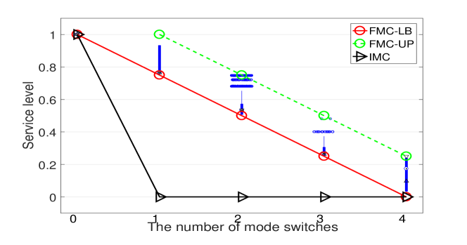
Figure 4: Service level of low-criticality tasks under the different number of mode switches.

As shown in Fig. 4, FMC can gracefully degrade the low-criticality service level as the number of mode switches increases. By contrast, IMC fails to respond to the variability in the workload. As long as not all high-criticality tasks overrun during run time, the execution budget determined by FMC always outperforms that of IMC.

Another interesting observation is that the collected run-time service levels are bounded by the red and green lines. This observation matches the FMC execution semantics presented in Section 3.2. In the $k^{\textit{th}}$ transition phase, the execution budget for low-criticality jobs will be reduced from $z^{k-1}\cdot{C_{i}^{LO}}$ to $z^{k}\cdot{C_{i}^{LO}}$. According to the FMC execution semantics, two cases can be considered:

• Case 1: Low-criticality jobs that have already exhausted their execution budget of $z^{k}\cdot{C_{i}^{LO}}$ at the transition point. Such jobs will be suspended immediately. In addition, these suspended jobs should have an execution time of less than $z^{k-1}\cdot{C_{i}^{LO}}$ by the $k$-th transition point. Otherwise, these jobs would have already been suspended when the system entered $(k-1)-level$ high-criticality mode. Therefore, the execution time of these jobs will be bounded in $[z^{k}\cdot{C_{i}^{LO}},z^{k-1}\cdot{C_{i}^{LO}})$.

• Case 2: Low-criticality jobs that have not yet exhausted their execution budget $z^{k}\cdot{C_{i}^{LO}}$. Such jobs will continue to run until their remaining time budget is used up. Therefore, these jobs will execute up to $z^{k}\cdot{C_{i}^{LO}}$.

From the above two cases, we can conclude that the execution time of these jobs in $k$-level high-criticality mode is bounded in $[z^{k}{C_{i}^{LO}},z^{k-1}{C_{i}^{LO}})$, as clearly shown in Fig. 4.

6.4 Run-time complexity

According to [4], for a task set containing $n$ tasks, the classic EDF-VD algorithm has a run-time complexity of $O(log\,n)$ per event for job arrival, job completion, and mode switching. Compared with EDF-VD [4], FMC-EDF-VD needs to implement only one additional operation during mode switching, that is, tuning the service levels for low-criticality tasks according to the specified strategy. For the uniform tuning strategy, the uniform service level $z_{k}$ can be directly computed with a complexity of $O(1)$ according to Thm. 6. For the dropping-off strategy, the dropping-off task can be determined via binary search with a complexity of $O(log\,n)$. Therefore, FMC-EDF-VD still has a run-time complexity of $O(log\,n)$ per event.

7 Evaluation

In this section, simulation experiments are presented to evaluate the performance of FMC. Our experiments are based on randomly generated MC tasks. We randomly generate task sets using the same approach as in [4, 12]. The various parameters are set as follows:

• The period $T_{i}$ of each task is an integer drawn uniformly at random from $[20,150]$.

• For each task $\tau_{i}$, low-criticality utilization $u_{i}^{LO}$ is a real number drawn at random from $[0.05,0.15]$.

• $R_{i}$ denotes the ratio of $u_{i}^{HI}/u_{i}^{LO}$, which is a real number drawn uniformly at random from $[2,3]$.

• pCri denotes the probability that a task $\tau_{i}$ is a high-criticality task, and we set this probability to $0.5$. If $\tau_{i}$ is a low-criticality task, then we set $C_{i}^{LO}=\lfloor{u_{i}^{LO}\cdot{T_{i}}}\rfloor$. Otherwise, we set $C_{i}^{LO}=\lfloor{u_{i}^{LO}\cdot{T_{i}}}\rfloor$ and $C_{i}^{HI}=\lfloor{u_{i}^{LO}\cdot{}R_{i}\cdot{}{T_{i}}}\rfloor$.

Given the utilization bound $u_{B}$, we generate one task at a time until the following conditions are both satisfied: (1) $u_{B}-0.05\leq\max\{u_{LO}^{LO}+u_{HI}^{LO},u_{HI}^{HI}\}\leq u_{B}$. (2) At least 3 high-criticality tasks have been generated.

The generated task set is evaluated for both off-line schedulability and on-line performance in terms of support for low-criticality task execution under six different schemes. These schemes include FMC with dropping off strategy proposed in this paper(’FMC’), Pfair-based scheme with using task grouping [22](’PF’), component-based scheme [12](’COM’), advanced EDF-VD scheduling of IMC systems [19](’IMC’), service adaption strategy that decreases the dispatch frequency of low-criticality tasks based on EDF-VD scheduling [16](’SA’), classic EDF-VD scheduling [4](’EDF-VD’).

The on-line low-criticality performance is measured as the percentage of finished LC jobs (denoted by PFJ), which is the same quantitative parameter used in [12]. PFJ is defined as the percentage of low-criticality jobs that are successfully finished by their deadlines. Each simulation is run for $10^{6}$ time units. The execution distribution presented in [23] is used to compute the probability that a high-criticality task $\tau_{i}$ will be executed beyond its low-criticality WCET. Due to schedulability performance differences among the compared schemes, the PFJ is obtained only when the taskset is schedulable for all compared schemes. The simulation process is detailed in Appendix C.

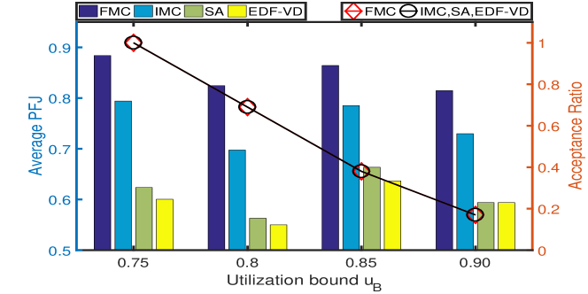
Figure 5: Comparison between FMC and schemes based on the global triggering.

7.1 Comparison with schemes based on the global triggering strategy

First, we demonstrate the effectiveness of FMC compared with the IMC, SA, and classic EDF-VD schemes, which use the global triggering strategy. In these three schemes, any overrun will trigger low-criticality tasks to statically reserve a constant degraded service level. For IMC and FMC, we consider the mandatory utilization $U_{LO}^{man}=0$ for the schedulability test. The schedulability test for the SA scheme [16] is a utilization-based test. Therefore, the IMC, SA, and classic EDF-VD schemes have the same schedulability. However, for some schedulable task sets, the SA scheme [16] cannot derive a suitable factor $y$ to increase the period of low-criticality tasks. For this case, we consider $y$ to be infinity, which means that all low-criticality jobs will be dropped when an overrun occurs.

For various utilization bounds $u_{B}\in\{0.75,0.8,0.85,0.9\}$, the average PFJ and system schedulability are compared. The results are shown in Fig. 5. The left axis shows the PFJ values achieved for low-criticality tasks, represented by the bar graphs, and the right axis shows the acceptance ratios, represented by the line graphs. From Fig. 5, we can observe the following trends: (1) FMC consistently outperforms the three other schemes in terms of support for low-criticality task execution. This is expected because schemes that use the global triggering strategy always consider the worst-case overrun workload, resulting in waste of unnecessary resources. By contrast, FMC can allocate resources based on the true overrun demands. (2) Compared with these three schemes based on the global triggering strategy, FMC achieves almost the same acceptance ratio. This means that FMC can achieve higher on-line low-criticality performance with negligibly reduced schedulability performance.

7.2 Comparison with the Pfair- and component-based schemes

Next, we will experimentally compare our approach to Pfair- and component-based schemes: PF [22] and COM [12]. For the component-based scheme COM [12], we use the same experiment setting as [12] and consider a two-component system with a high-criticality component $\mathbb{C_{H}}$ and a low-criticality component $\mathbb{C_{L}}$. All the high-criticality tasks are allocated to $\mathbb{C_{H}}$. Each low-criticality task can be allocated to either $\mathbb{C_{H}}$ or $\mathbb{C_{L}}$. Since the performance of the scheme presented in [12] depends on a tolerance limit $TL$, we generate the result of component-based scheme  [12] for various values of the tolerance limit $TL=\{0,\lfloor{0.25|H|}\rfloor,\lfloor{0.5|H|}\rfloor,\lfloor{0.75|H|}\rfloor,|H|\}$, where $|H|$ denotes the number of high-criticality tasks. For the Pfair-based scheme [22], a two-phased scheduling strategy is implemented for comparison.

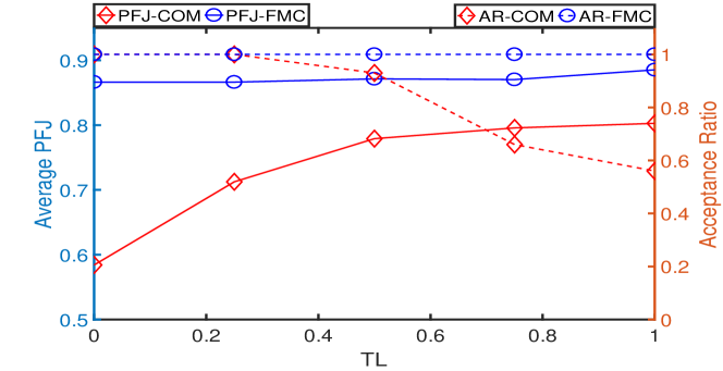
(a) $u_{B}=0.75$

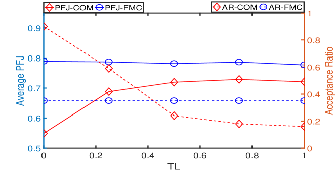
(b) $u_{B}=0.85$

Figure 6: Comparison between component-based scheme and FMC.

Comparison with component-based scheme COM [12]: The performance results of COM and FMC are presented in Fig. 6(a) and Fig. 6(b) with different settings on $u_{B}$. In these figures, x-axis denotes the varying value of $TL$, whereas the left and right y-axis present the average PFJ and acceptance ratio, respectively. As shown in Fig. 6, FMC consistently outperforms COM in terms of support for low-criticality execution. This performance gain is achieved by the fact that COM adopts pessimistic dropping-off strategies in internal and external mode-switch levels. In COM, all low-criticality tasks in $\mathbb{C_{H}}$ will be abandoned once any overrun occurs and thus results in resource under-utilization. As a comparison, FMC drops off low-criticality tasks as the demand and therefore can achieve better execution support for low-criticality tasks. Besides, we can observe that there is a performance trade-off between PFJ and acceptance ratio in COM. The reason for this trend is that a higher $TL$ in COM requires additional resources to support low-criticality executions but generally implies lower schedulability, and the converse also holds. When we consider the TL configuration on which the same scheduability performance can be achieved by FMC and COM, FMC can support more than 25% and 15% low-criticality tasks to finish the deadline compared to COM under different $u_{B}$ settings, respectively.

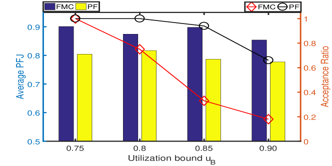
Figure 7: Comparison between Pfair-based scheme and FMC.

Comparison with Pfair-based scheme PF [22]: Fig. 7 shows the compared results for FMC and PF. Compared with PF, FMC can achieve a better execution support for low-criticality tasks but with inferior schedulability, as shown in Fig. 7. The reason for the gain in low-criticality task execution support is that the Pfair scheduling tends to evenly distribute the quanta of tasks over time, resulting in more unfinished jobs at mode-switching points.

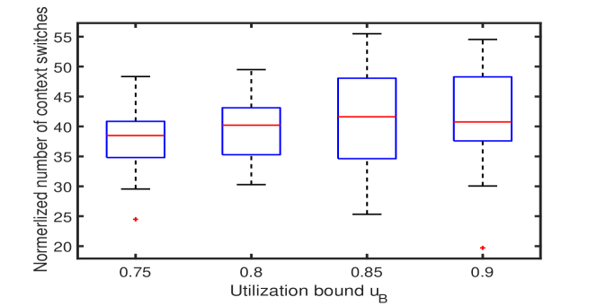
Figure 8: Context switches for FMC and Pfair-based scheme.

Regarding schedulability inferiority, we mainly attribute this expected inferiority to the theoretical optimality of Pfair scheduling in terms of schedulability performance [14]. In fact, this optimality is achieved at the cost of a high scheduling overhead by quantum-length sub-tasks partitioning and the enforcement of proportional progress. In fact, this schedulability deficit of FMC can be compensated by significantly reduced context-switching overheads compared with PF. Here, we present simulation results to show the compared context-switch numbers. Fig. 8 presents the number of context switches for the Pfair-based scheme, which is normalized with respect to the number for FMC. The results confirm the significant reduction of context switches by FMC. The Pfair-based scheme requires 38.0 to 41.3 times the number of context switches required in FMC for different utilization settings.

7.3 Graceful service level degradation

In the case study presented above, we have demonstrated the gradual service level degradation property of FMC, that is, the degradation in the service levels for low-criticality tasks as the number of mode switch increases. Now, we validate this trend in a generic simulation. The uniform tuning strategy is applied to randomly generated task sets. We use the task generator introduced above to generate 100 task sets in which $u_{B}$ is randomly selected from $[0.75,0.9]$. A generated task set is accepted for simulation when the following two additional conditions are satisfied: (1) the task set can be scheduled by FMC, and (2) the task set contains 5 high-criticality tasks. The degraded low-criticality jobs under various task sets are classified according to the number of mode switches.

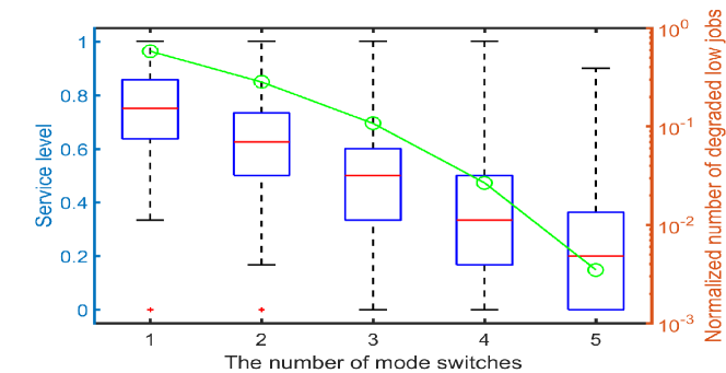
Figure 9: Service degradation in generic simulation.

The simulation results are shown in Fig. 9. The left and right y-axis present the service level and the normalized number of service-degraded low-criticality jobs, respectively. To reveal the distribution of service levels for service-degraded low-criticality jobs, the service levels are represented in the form of box-whisker plots. The results shown in Fig. 9 confirm the observations made in Section 6.3. For almost all low-criticality task jobs, the graceful degradation property is clearly demonstrated except for a few corner cases. Furthermore, the results in terms of the percentages of service-degraded low-criticality jobs also confirm that the likelihood of all high-criticality tasks exhibiting the high-criticality behavior is very low. Only 0.35% of service-degraded low-criticality jobs are affected by this worst-case overrun scenario. By contrast, 96.9% of service-degraded low-criticality jobs are impacted by mode-switch scenarios with mode switches$\leq{}3$. For this vast majority of cases, FMC needs to allocate additional resources to only a subset of the high-criticality tasks based on their demands and therefore can provide better and more graceful service degradation.

8 Conclusion and future work

Most previous theoretical work on scheduling in mixed-criticality systems has adopted impractical assumptions: once any high-criticality task overruns, all low-criticality tasks are suspended and all other high-criticality tasks are required to exhibit high-criticality behaviors. In this paper, we propose a more flexible MC model (FMC) with EDF-VD scheduling, in which the above issues are addressed. In this model, the transitions of all high-criticality tasks are independent and the service levels of low-criticality tasks can be adaptively tuned in accordance with the true overruns of the high-criticality tasks. A utilization-based schedulability test condition is successfully derived for the FMC systems. Numerical results are presented to illustrate the improved service levels for low-criticality tasks during run time.

For the next step, we are interested in implementing the proposed approach on real-time operating system and evaluating its performance. Furthermore, another interesting future work includes investigations on: (1) integrating of FMC and fault tolerance techniques to develop optimal resource allocation strategies for assurances against different types of faults; (2) integrating the slack reclamation schemes into FMC for further performance improvement.

Appendix A Derivation protocol

This section presents the detailed proofs for the derivation protocol presented in Eqn. (5.3.3) and Eqn. (5.3.3). The rules for deriving intermediate upper bounds for different execution scenarios are specified as follows:

Rule 1

If no $k$-carry-over job of low-criticality task $\tau_{i}$ exists at the $k^{\textit{th}}$ mode-switching point $\hat{t}^{k}$, then the intermediate upper bound $\sup\{\eta_{i}^{k}(0,t_{f})\}$ is computed as

$$\sup\{\eta_{i}^{k}(0,t_{f})\}=\sup\{\eta_{i}^{k}(0,d_{i}^{l})\}+(t_{f}-\hat{t}^{k})\cdot{}z_{i}^{k}\cdot{}u_{i}^{LO}$$ (31)

where $d_{i}^{l}$ denotes the absolute deadline of the last job of $\tau_{i}$ during $[0,t_{f}]$.

Proof:

Since no $k$-carry-over job of $\tau_{i}$ exists at $\hat{t}^{k}$, we know that $d_{i}^{l}<\hat{t}^{k}$. Therefore, $\sup\{\eta_{i}^{k}(0,d_{i}^{l})\}$ is sufficient to bound $\eta_{i}^{k}(0,t_{f})$. Since $(t_{f}-\hat{t}^{k})\cdot{}z_{i}^{k}\cdot{}u_{i}^{LO}>0$, we know that $\sup\{\eta_{i}^{k}(0,d_{i}^{l})\}+(t_{f}-\hat{t}^{k})\cdot{}z_{i}^{k}\cdot{}u_{i}^{LO}$ is also an upper bound. ∎

Rule 2

If a $k$-carry-over job of low-criticality task $\tau_{i}$ exists at the $k^{\textit{th}}$ mode-switching point $\hat{t}^{k}$, then the intermediate upper bound $\sup\{\eta_{i}^{k}(0,t_{f})\}$ is computed as

$$\sup\{\eta_{i}^{k}(0,t_{f})\}=\sup\{\eta_{i}^{k}(0,d_{i}^{k})\}+(t_{f}-d_{i}^{k})\cdot{}z_{i}^{k}\cdot{}u_{i}^{LO}$$ (32)

Proof:

$\sup\{\eta_{i}^{k}(0,t_{f})\}$ can be calculated as $\sup\{\eta_{i}^{k}(0,d_{i}^{k})\}+\sup\{\eta_{i}^{k}(d_{i}^{k},t_{f})\}$. Since $(t_{f}-d_{i}^{k})\cdot{}z_{i}^{k}\cdot{}u_{i}^{LO}$ is sufficient to bound $\eta_{i}^{k}(d_{i}^{k},t_{f})$ according to Prop. 1, we know that $\sup\{\eta_{i}^{k}(0,d_{i}^{k})\}+(t_{f}-d_{i}^{k})\cdot{}z_{i}^{k}\cdot{}u_{i}^{LO}$ can be used as an upper bound. ∎

Rule 3

For a $k$-carry-over job of low-criticality task $\tau_{i}$, if $\eta_{i}^{k}(a_{i}^{k},\hat{t}^{k})\neq{0}$, then the intermediate upper bound $\sup\{\eta_{i}^{k}(a_{i}^{k},d_{i}^{k})\}$ will be computed as follows:

$$\sup\{\eta_{i}^{k}(a_{i}^{k},d_{i}^{k})\}={(d_{i}^{k}-a_{i}^{k})\cdot{z_{i}^{k-j}}\cdot{u_{i}^{LO}}}$$ (33)

where $z_{i}^{k-j}$ is the service level after the last mode switch occurring before $a_{i}^{k}$.

Proof:

According to Fig. 2, $j$ mode switches may occur during the interval $(a_{i}^{k},\hat{t}^{k})$. Recall the assumption $z_{i}^{k}\leq{z_{i}^{k-1}}$ ($\forall k$) made in Section 3; based on this assumption, we have $z_{i}^{k-j}\geq{}z_{i}^{k-(j-1)}\geq{}\cdots\geq{}z_{i}^{k}$. When the system switches modes at $\hat{t}^{k_{0}}$ ($k-(j-1)\leq{k_{0}}\leq{k}$), the execution budget will be reduced from $z_{i}^{k_{0}-1}\cdot{c_{i}^{LO}}$ to $z_{i}^{k_{0}}\cdot{c_{i}^{LO}}$. Therefore, the maximum cumulative execution is achieved when the $k$-carry-over job has completed its $z_{i}^{k-j}\cdot C_{i}^{LO}$ execution before time instant $\hat{t}^{k-(j-1)}$, which is the time of the first mode switch occurring after $a_{i}^{k}$. Therefore, in this case, the $k$-carry-over job can be bounded by $(d_{i}^{k}-a_{i}^{k})\cdot{z_{i}^{k-j}}\cdot{u_{i}^{LO}}$. ∎

Rule 4

For a $k$-carry-over job of low-criticality task $\tau_{i}$, if $\eta_{i}^{k}(a_{i}^{k},\hat{t}^{k})={0}$, the intermediate upper bound $\sup\{\eta_{i}^{k}(a_{i}^{k},d_{i}^{k})\}$ will be computed as follows:

$$\sup\{\eta_{i}^{k}(a_{i}^{k},d_{i}^{k})\}={(d_{i}^{k}-a_{i}^{k})\cdot{z_{i}^{k}}\cdot{u_{i}^{LO}}}$$ (34)

Proof:

Since the $k$-carry-over job has not been executed before $\hat{t}^{k}$ ($\eta_{i}^{k}(a_{i}^{k},\hat{t}^{k})={0}$), it must exhaust its execution budget $z_{i}^{k}\cdot{}C_{i}^{LO}$ after the mode-switching time instant $\hat{t}^{k}$. Therefore, the maximum cumulative execution at the current time can be found to be $(d_{i}^{k}-a_{i}^{k})\cdot{z_{i}^{k}}\cdot{u_{i}^{LO}}$. ∎

Appendix B The derivation of $N^{k}_{\gamma}$ in Eqn. (21)

The following is the detailed derivation of the upper bound on the total cumulative execution time $N^{k}_{\gamma}$.

$$N^{k}_{\gamma}=N^{k}_{\gamma_{LO}}+N^{k}_{\gamma_{HI}^{HI}(\hat{t}^{k})}+N^{k}_{\gamma_{HI}^{LO}(\hat{t}^{k})}$$

$$\leq{} \underbrace{\sum_{\tau_{i}\in\gamma_{LO}}\bigg{(}t_{f}u_{i}^{LO}+\sum_{j=1}^{k}{((t_{f}-a_{\hat{t}^{j}})(1-x)(z_{i}^{j}-z_{i}^{j-1})u_{i}^{LO})}\bigg{)}}_{N^{k}_{\gamma_{LO}}}$$

$$+\underbrace{\sum_{j=1}^{k}{(a_{\hat{t}^{j}}\cdot{}u_{\hat{t}^{j}}^{LO}+(t_{f}-a_{\hat{t}^{j}})\cdot{}u_{\hat{t}^{j}}^{HI})}}_{N^{k}_{\gamma_{HI}^{HI}(\hat{t}^{k})}}+\underbrace{\sum_{\tau_{i}\in\gamma_{HI}^{LO}}{\frac{t_{f}}{x}\cdot{}u_{i}^{LO}}}_{N^{k}_{\gamma_{HI}^{LO}(\hat{t}^{k})}}$$

$$= \underline{t_{f}u_{LO}^{LO}}+\sum_{j=1}^{k}{(t_{f}-a_{\hat{t}^{j}})(1-x)(u_{LO}^{j}-u_{LO}^{j-1})}$$

$$+\sum_{j=1}^{k}{(a_{\hat{t}^{j}}\cdot{}u_{\hat{t}^{j}}^{LO}+(t_{f}-a_{\hat{t}^{j}})\cdot{}u_{\hat{t}^{j}}^{HI})}+\sum_{\tau_{i}\in\gamma_{HI}^{LO}}{\frac{t_{f}}{x}\cdot{}u_{i}^{LO}}$$

$$= \ (Consider\ a_{0}=\frac{\sum_{j=1}^{k}{a_{\hat{t}^{j}}u_{\hat{t}^{j}}^{LO}}}{\sum_{j=1}^{k}{u_{\hat{t}^{j}}^{LO}}})$$

$$\underline{(t_{f}-a_{0})u_{LO}^{LO}+a_{0}u_{LO}^{LO}}+\sum_{j=1}^{k}{(t_{f}-a_{\hat{t}^{j}})(1-x)(u_{LO}^{j}-u_{LO}^{j-1})}$$

$$+\sum_{j=1}^{k}{(a_{\hat{t}^{j}}\cdot{}u_{\hat{t}^{j}}^{LO}+(t_{f}-a_{\hat{t}^{j}})\cdot{}u_{\hat{t}^{j}}^{HI})}+\sum_{\tau_{i}\in\gamma_{HI}^{LO}}{\frac{t_{f}}{x}\cdot{}u_{i}^{LO}}$$

$$\leq \ (Since\ u_{LO}^{LO}+\frac{u_{HI}^{LO}}{x}\leq{1}\ and\ x<1)$$

$$(t_{f}-a_{0})u_{LO}^{LO}+\underline{a_{0}(1-\frac{u_{HI}^{LO}}{x})}+\sum_{j=1}^{k}{(t_{f}-a_{\hat{t}^{j}})(1-x)(u_{LO}^{j}-u_{LO}^{j-1})}$$

$$+\sum_{j=1}^{k}{(\underline{\frac{a_{\hat{t}^{j}}}{x}u_{\hat{t}^{j}}^{LO}}+(t_{f}-a_{\hat{t}^{j}})u_{\hat{t}^{j}}^{HI})}+\sum_{\tau_{i}\in\gamma_{HI}^{LO}}{\frac{t_{f}}{x}u_{i}^{LO}}$$

$$= \ (Since\ u_{HI}^{LO}=\sum_{j=1}^{k}{u_{\hat{t}^{j}}^{LO}}+\sum_{\tau_{i}\in\gamma_{HI}^{LO}}{u_{i}^{LO}})$$

$$t_{f}+(t_{f}-a_{0})(u_{LO}^{LO}-1)+\sum_{j=1}^{k}{(t_{f}-a_{\hat{t}^{j}})(1-x)(u_{LO}^{j}-u_{LO}^{j-1})}$$

$$+ \underline{\sum_{j=1}^{k}{\frac{a_{\hat{t}^{j}}u_{\hat{t}^{j}}^{LO}-a_{0}u_{\hat{t}^{j}}^{LO}}{x}}}+\sum_{j=1}^{k}{(t_{f}-a_{\hat{t}^{j}})u_{\hat{t}^{j}}^{HI}}+\underline{\sum_{\tau_{i}\in\gamma_{HI}^{LO}}{\frac{t_{f}-a_{0}}{x}u_{i}^{LO}}}$$

$$= \ (Since\ \sum_{j=1}^{k}{(a_{\hat{t}^{j}}u_{\hat{t}^{j}}^{LO}-a_{0}u_{\hat{t}^{j}}^{LO})}=0)$$

$$t_{f}+(t_{f}-a_{0})(u_{LO}^{LO}-1)+\sum_{j=1}^{k}{(t_{f}-a_{\hat{t}^{j}})(1-x)(u_{LO}^{j}-u_{LO}^{j-1})}$$

$$+\sum_{j=1}^{k}{(t_{f}-a_{\hat{t}^{j}})u_{\hat{t}^{j}}^{HI}}+\sum_{\tau_{i}\in\gamma_{HI}^{LO}}{\frac{t_{f}-a_{0}}{x}u_{i}^{LO}}$$

$$= \ (Since\ t_{f}-a_{0}=\frac{\sum_{j=1}^{k}(t_{f}-a_{\hat{t}^{j}})u_{\hat{t}^{j}}^{LO}}{\sum_{j_{0}=1}^{k}u_{\hat{t}^{j_{0}}}^{LO}})$$

$$t_{f}+\sum_{j=1}^{k}(t_{f}-a_{\hat{t}^{j}})\bigg{(}\frac{u_{\hat{t}^{j}}^{LO}}{\sum_{j_{0}=1}^{k}u_{\hat{t}^{j_{0}}}^{LO}}(u_{LO}^{LO}-1)+(1-x)(u_{LO}^{j}-u_{LO}^{j-1})$$

$$+u_{\hat{t}^{j}}^{HI}+\frac{u_{\hat{t}^{j}}^{LO}}{\sum_{j_{0}=1}^{k}u_{\hat{t}^{j_{0}}}^{LO}}\sum_{\tau_{i}\in\gamma_{HI}^{LO}}\frac{u_{i}^{LO}}{x}\bigg{)}$$

$$= \ (Since\ u_{HI}^{LO}=\sum_{j=1}^{k}{u_{\hat{t}^{j}}^{LO}}+\sum_{\tau_{i}\in\gamma_{HI}^{LO}}{u_{i}^{LO}})$$

$$t_{f}+\sum_{j=1}^{k}(t_{f}-a_{\hat{t}^{j}})\bigg{(}u_{\hat{t}^{j}}^{HI}-\frac{u_{\hat{t}^{j}}^{LO}}{x}+(1-x)(u_{LO}^{j}-u_{LO}^{j-1})$$

$$+\frac{u_{\hat{t}^{j}}^{LO}}{\sum_{j_{0}=1}^{k}u_{\hat{t}^{j_{0}}}^{LO}}(u_{LO}^{LO}-1+\frac{u_{HI}^{LO}}{x})\bigg{)}$$

$$\leq \ (Since\ u_{LO}^{LO}-1+\frac{u_{HI}^{LO}}{x}\leq{0}\ and\ \sum_{j_{0}=1}^{k}u_{\hat{t}^{j_{0}}}^{LO}\leq{}u_{HI}^{LO})$$

$$t_{f}+\sum_{j=1}^{k}(t_{f}-a_{\hat{t}^{j}})\bigg{(}u_{\hat{t}^{j}}^{HI}-\frac{u_{\hat{t}^{j}}^{LO}}{x}+(1-x)(u_{LO}^{j}-u_{LO}^{j-1})$$

$$+\frac{u_{\hat{t}^{j}}^{LO}}{u_{HI}^{LO}}(u_{LO}^{LO}-1+\frac{u_{HI}^{LO}}{x})\bigg{)}$$

$$= t_{f}+\sum_{j=1}^{k}(t_{f}-a_{\hat{t}^{j}})\bigg{(}u_{\hat{t}^{j}}^{HI}+(1-x)(u_{LO}^{j}-u_{LO}^{j-1})+\frac{u_{\hat{t}^{j}}^{LO}}{u_{HI}^{LO}}(u_{LO}^{LO}-1)\bigg{)}$$

Appendix C Simulation Framework

In this section, we will present the simulation framework which faithfully emulate real time execution behaviors of mixed criticality tasks. This simulation framework enables us to evaluate various advanced mixed criticality scheduling algorithms and to obtain performance statistics for algorithms evaluation. In the simulation, the workload trace of jobs are firstly generated. All the compared approaches are tested by the same workload trace in the simulation, such that the fairness can be guaranteed. During the simulation, the statistics entity will collect data from the simulation to calculate different metrics for the compared algorithms. In our simulation, as long as low-criticality job do not finish its $C_{i}^{LO}$, this low-criticality job will be considered as the job without completion. The main aspects of the simulation process will be described as follows.

Workload Trace Generation: For the sake of fairness, we generate the workload trace of jobs according to task specification and use this workload trace to uniformly test the compared approaches. In this process, the arrival time, execution time, and overruns of jobs are generated before the simulation. To validate the runtime scheduability in the worst-case scenario, all jobs are released with minimum job-arrival interval and are executed with the worst-case execution time for stress testing. The overruns of each high-criticality jobs are randomly generated according to the overrun probability, which is computed according to execution distribution presented in [23].

Run-time Simulation: The system tick is the time unit that causes the scheduler to run and process events. In our simulation, we emulate real time execution behaviors of mixed criticality tasks based on system tick. The possible events are processed according to the following rules:

• Newly-arrived job: If the system is in low-criticality mode, the newly-arrived job will be inserted into the queue $Q$ with modified deadline and unmodified execution budgets. Otherwise, high-criticality jobs with be inserted with unmodified deadline and execution budgets $C_{i}^{H}$, while low-criticality jobs will be inserted with degraded execution budgets $z_{i}^{k}\cdot{}C_{i}^{L}$.

• Job completion: If the job reaches its execution budget, delete the job from the queue $Q$. Record the performance data of the jobs.

• Preemption and consume time: Find the job with minimum deadline in $Q$ to execute and consume the current time slot. If the current job is different with the one executed in last time unit, the preemption is identified.

• Overrun and mode switches: If high-criticality tasks overrun its execution budgets $C_{i}^{LO}$, transit system to high-criticality mode and update the service level $z_{i}^{k}$ for each low-criticality task.

• Switch back: If $Q$ is empty, the idle interval is detected. The system will be transit back to low-criticality mode by resetting $z_{i}^{k}=1$ for each low-criticality task.

Similarly, this simulation framework can be easily extended for other compared approaches by replacing the degradation strategy in the simulation.

Appendix D The screen-shot of submission

The submission history is shown in Fig. 10.

Figure 10: Submission Information on TC.

References

- [1] S. Baruah et al. Towards the design of certifiable mixed-criticality systems. In 2010 16th IEEE Real-Time and Embedded Technology and Applications Symposium, 2010.
- [2] S. Baruah et al. Mixed-criticality scheduling of sporadic task systems. In the 19th European Conference on Algorithms, 2011.
- [3] S. Baruah et al. Response-time analysis for mixed criticality systems. In 2011 IEEE 32nd Real-Time Systems Symposium, 2011.
- [4] S. Baruah et al. The preemptive uniprocessor scheduling of mixed-criticality implicit-deadline sporadic task systems. In 2012 24th Euromicro Conference on Real-Time Systems, 2012.
- [5] S. Baruah et al. Preemptive uniprocessor scheduling of mixed-criticality sporadic task systems. Journal of the ACM, 62(2), 2015.
- [6] P. Binns. Incremental rate monotonic scheduling for improved control system performance. In 3rd IEEE Real-Time Technology and Applications Symposium, 1997.
- [7] A. Burns et al. Towards a more practical model for mixed criticality systems. In 1st International Workshop on Mixed Criticality Systems, pages 1–6, 2013.
- [8] A. Burns et al. Mixed criticality systems-a review. University of York, Technical Report, 2015.
- [9] H. Chishiro et al. Practical imprecise computation model: Theory and practice. In 2014 IEEE 17th International Symposium on Object/Component/Service-Oriented Real-Time Distributed Computing, 2014.
- [10] W. Feng et al. An extended imprecise computation model for time-constrained speech processing and generation. In IEEE Workshop on Real-Time Applications, 1993.
- [11] C. A. Floudas. Deterministic Global Optimization: Theory, Methods and Applications. Springer, 2005.
- [12] X. Gu et al. Resource efficient isolation mechanisms in mixed-criticality scheduling. In 2015 27th Euromicro Conference on Real-Time Systems, 2015.
- [13] C. C. Han et al. A fault-tolerant scheduling algorithm for real-time periodic tasks with possible software faults. IEEE Transactions on Computers, 2003.
- [14] P. Holman et al. Group-based pfair scheduling. Real-Time Systems, 2006.
- [15] P. Huang et al. Interference constraint graph: A new specification for mixed-criticality systems. In 2013 IEEE 18th Conference on Emerging Technologies Factory Automation, pages 1–8, 2013.
- [16] P. Huang et al. Service adaptions for mixed-criticality systems. In 2014 19th Asia and South Pacific Design Automation Conference, 2014.
- [17] ISO 26262:Road vehicles. http://www.iso.org/iso/.
- [18] K.-J. Lin et al. Imprecise results: Utilizing partial comptuations in real-time systems. In Real-Time Systems Symposium, 1987.
- [19] D. Liu et al. Edf-vd scheduling of mixed-criticality system with degraded quality guarantees. In 2016 IEEE 32nd Real-Time Systems Symposium, 2016.
- [20] J. W. S. Liu et al. Imprecise computations. 1994.
- [21] R. Rajkumar et al. A resource allocation model for qos management. In 1997 IEEE Real-Time Systems Symposium, 1997.
- [22] J. Ren et al. Mixed-criticality scheduling on multiprocessors using task grouping. In 2015 27th Euromicro Conference on Real-Time Systems, pages 25–34, 2015.
- [23] F. Santy, L. George, P. Thierry, and J. Goossens. Relaxing mixed-criticality scheduling strictness for task sets scheduled with fp. In 2012 24th Euromicro Conference on Real-Time Systems, 2012.
- [24] H. Su et al. An elastic mixed-criticality task model and its scheduling algorithm. In Design, Automation Test in Europe Conference Exhibition, 2013.
- [25] H. Su et al. Service guarantee exploration for mixed-criticality systems. In 2014 IEEE 20th International Conference on Embedded and Real-Time Computing Systems and Applications, 2014.
- [26] S. Vestal. Preemptive scheduling of multi-criticality systems with varying degrees of execution time assurance. In 2007 28th IEEE International Real-Time Systems Symposium, 2007.
- [27] D. Zhu et al. Multiple-resource periodic scheduling problem: how much fairness is necessary? In 24th IEEE Real-Time Systems Symposium, 2003.