NONLINEAR ELECTRODYNAMICS, REGULAR BLACK HOLES
AND WORMHOLES

Abstract

We consider spherically symmetric configurations in general relativity, supported by nonlinear electromagnetic fields with gauge-invariant Lagrangians depending on the single invariant $f=F_{\mu\nu}F^{\mu\nu}$. Static black hole (BH) and solitonic solutions are briefly described, both with only an electric or magnetic charge and with both nonzero charges (the dyonic ones). It is stressed that only pure magnetic solutions can be completely nonsingular. For dyonic systems, apart from a general scheme of obtaining solutions in quadratures for an arbitrary Lagrangian function $L(f)$, an analytic solution is found for the truncated Born-Infeld theory (depending on the invariant $f$ only). Furthermore, considering spherically symmetric metrics with two independent functions of time, we find a natural generalization of the class of wormholes found previously by Arellano and Lobo with a time-dependent conformal factor. Such wormholes are shown to be only possible for some particular choices of the function $L(f)$, having no Maxwell weak-field limit.

PACS numbers: 04.70.Bw, 04.20.Jb, 04.20.Gz

1 Introduction

Nonlinear electrodynamics (NED) appeared in the 1930s with Born and Infeld’s effort to remove the central singularity of a point charge and the related energy divergence by generalizing Maxwell’s theory [1], and the version of NED put forward by Heisenberg and Euler, motivated by particle physics [2]. It was further extended by Plebanski [3] in the framework of special relativity, including an arbitrary function of the electromagnetic field invariants.

The interest in NED in modern studies is to a large extent motivated by the discovery that some kinds of NED appear as limiting cases of certain models of string theory [4, 5]. It is also clear that the real electromagnetic field should lose its linearity at high energies due to interactions with other physical fields, and NED theories may be considered as a simplified phenomenological description of these interactions. On the other hand, NED as a possible material source of gravity is able to create various nonsingular geometries of interest, in particular, regular black holes (BHs) and starlike or solitonlike configurations in the framework of general relativity (GR) and alternative theories.

Among such models, the simplest are spherically symmetric ones, where the only possible kinds of electromagnetic fields are radial electric and radial magnetic fields. Such solutions are widey discussed in the literature, beginning probably with the paper by Pellicer and Torrence [6] where a general static solution was obtained for configurations with an electric field only. In Ref. B-Shi, a no-go theorem was proved showing that if NED is specified by a Lagrangian function $L(f)$ (where $f=F_{\mu\nu}F^{\mu\nu}$, and $F_{\mu\nu}$ is the Maxwell tensor), there is no such function $L(f)$ having a Maxwell weak-field limit ($L\sim f$ as $f\to 0$) that a static, spherically symmetric solution of GR with an electric field has a regular center. This theorem was further extended to static dyonic configurations, with both electric and magnetic fields [8], and it was further shown [8, 9] that in numerous electric solutions describing configurations with or without horizons (that is, BH or solitonic ones), having a regular center and a Reissner-Nordström (RN) behavior at large radii $r$, there are different Lagrangian functions $L(f)$ at large and small $r$: at large $r$ we have $L\sim f$ whereas at small $r$ the theory is strongly non-Maxwell ($f\to 0$ but $L_{f}\to\infty$, in agreement with the no-go theorem).

Meanwhile,[8] purely magnetic regular configurations, both BH and solitonic ones, are possible and are readily obtained under the condition $L(f)\to L_{\infty}<\infty$ as $f\to\infty$. Electric models with the same regular metrics can be obtained from the magnetic ones using the so-called FP duality [8] (not to be confused with the familiar electric-magnetic duality in Maxwell’s theory) that connects solutions with the same metric corresponding to different NED theories. Unlike the magnetic solutions, the electric ones suffer serious problems connected with multivaluedness of $L(f)$ and a singular behavior of the electromagnetic fields on the branching surfaces [8].

Many results of interest were obtained since then, for a brief review see, e.g., Ref. 17-dyon and references therein. Among them let us point out a description of models with a kind of phase transition allowing one to circumvent the above no-go theorem [11], an extension of static, spherically symmetric NED solutions to GR with a nonzero cosmological constant $\Lambda$,[12] thermodynamic properties of regular NED BHs [13, 14, 15], cylindrically [16] and axially [17, 18] symmetric regular GR/NED configurations and evolving wormhole models,[19, 20, 21] the stability properties of NED BHs,[22, 23, 24] and quantum effects in their fields.[25, 26]. One can also mention numerous studies of special cases of electric and magnetic solutions, their potential observational properties like gravitational lensing, particle motion and matter accretion in the fields of NED BHs, their counterparts in scalar-tensor, $f(R)$ and multidimensional theories of gravity, inclusion of dilaton-like interactions, non-Abelian fields, constructions with thin shells, etc., but the corresponding list of references would be too long. The subject probably deserves a comprehensive review.

In this paper we discuss some recent progress concerning two subjects in the framework of NED coupled to GR: static, spherically symmetric dyonic solutions and spherically symmetric evolving wormholes. The dyonic solutions are inevitably singular at the center, as follows from the no-go theorem [8], but they are of interest as the first examples of this kind of solutions.[10]. For completeness and comparison, pure electric and magnetic solutions are also briefly described.

As to wormholes as two-way tunnels or shortcuts between different universes or different, otherwise distant regions of the same universe, their possible existence and properties are widely discussed, see, e.g., Refs. viss-book–WH-book for reviews. Wormholes are of interest not only as a perspective “means of transportation” but also as possible time machines or accelerators [31, 29]. Spherical symmetry is a natural simple framework for wormhole geometry, and most of known exact wormhole solutions in GR and alternative theories of gravity (e.g., Refs. k73–BS-extra and many others) are static, spherically symmetric. However, NED as a source of gravity in GR cannot support static wormholes because it does not provide the necessary violation of the Null Energy Condition (NEC). Only by considering evolving conformally static space-times it has been possible to obtain some examples of NED/GR wormhole solutions [19]. In this paper, the approach developed in Refs. Arel-06–Arel-09 is extended to a more general class of time-dependent metrics, containing two functions of time and somewhat similar to Kantowski-Sachs cosmologies.

After presenting some general relations valid for both static and time-dependent NED/GR configurations (Section 2), in Section 3 we briefly describe all three types of static solutions: magnetic, electric and dyonic ones, following the previous papers, Refs. k-NED and 17-dyon. In Section 4 we obtain and discuss a new class of nonstatic spherically symmetric wormhole solutions, containing those of Arellano and Lobo as a special case. Section 5 is a conclusion.

2 Basic equations. FP duality

We start with the action

$$S={{\displaystyle\frac{1}{2}}}\int\sqrt{-g}d^{4}x[R-L(f)],$$ (1)

where $R$ is the Ricci scalar, $L(f)$ is an arbitrary functions, and units are used with $c=8\pi G=1$. The Einstein equations can be written, as usual, in two equivalent forms

$${}G_{\mu}^{\nu}\equiv R_{\mu}^{\nu}-{{\textstyle\frac{1}{2}}}\delta_{\mu}^{\nu}R=-T_{\mu}^{\nu},\qquad{\rm or}$$

$${}\qquad R_{\mu}^{\nu}=-(T_{\mu}^{\nu}-{{\textstyle\frac{1}{2}}}\delta_{\mu}^{\nu}T^{\alpha}_{\alpha}),$$ (2)

where $T_{\mu}^{\nu}$ is the stress-energy tensor (SET), which in the theory (1) is given by ($L_{f}\equiv dL/df$)

$$T_{\mu}^{\nu}=-2L_{f}F_{\mu\alpha}F^{\nu\alpha}+{{\textstyle\frac{1}{2}}}\delta_{\mu}^{\nu}L(f).$$ (3)

The metric is taken in the general spherically symmetric form

$$ds^{2}=A(x,t)dt^{2}-B(x,t)dx^{2}-r^{2}(x,t)d\Omega^{2},\hskip 28.45274ptd\Omega^{2}=d\theta^{2}+\sin^{2}\theta d\phi^{2}.$$ (4)

The only nonzero components of $F_{\mu\nu}$ compatible with spherical symmetry are $F_{tr}=-F_{rt}$ (a radial electric field) and $F_{\theta\phi}=-F_{\phi\theta}$ (a radial magnetic field). The Maxwell-like equations $\nabla_{\mu}(L_{f}F^{\mu\nu})=0$ and the Bianchi identities $\nabla_{\mu}{}^{*}F^{\mu\nu}=0$ for the dual field ${}^{*}F^{\mu\nu}$ lead to

$$r^{2}\sqrt{AB}L_{f}F^{tr}=q_{e},\hskip 28.45274ptF_{\theta\phi}=q_{m}\sin\theta,$$ (5)

where $q_{e}$ and $q_{m}$ are the electric and magnetic charges, respectively.

Accordingly, the only nonzero SET components are

$${}T^{t}_{t}=T^{r}_{r}={{\textstyle\frac{1}{2}}}L+f_{e}L_{f},$$

$${}T^{\theta}_{\theta}=T^{\phi}_{\phi}={{\textstyle\frac{1}{2}}}L-f_{m}L_{f},$$ (6)

and the invariant $f$ is the difference $f=f_{m}-f_{e}=2({\bf B}^{2}-{\bf E}^{2})$, where

$${}f_{e}=2F_{tr}F^{rt}=2{\bf E}^{2}=\frac{2q_{e}^{2}}{L_{f}^{2}r^{4}}\geq 0,$$

$${}f_{m}=2F_{\theta\phi}F^{\theta\phi}=2{\bf B}^{2}=\frac{2q_{m}^{2}}{r^{4}}\geq 0,$$ (7)

${\bf E}$ and ${\bf B}$ being the absolute values of the radial electric field strength and magnetic induction, respectively, measured by an observer at rest in the reference frame under consideration.

The SET (2) has the important properties $T^{t}_{t}=T^{x}_{x}$ and $T^{t}_{x}=0$; the latter means the absence of radial energy flows, which is in turn related to the absence of electromagnetic monopole radiation. Taken together, these two properties define a kind of matter sometimes called Dymnikova’s vacuum [39, 40], its evident vacuum-like property is that its SET structure is insensitive to any transformations of the coordinates $x^{0}=t$ and $x^{1}=x$; in other words, all reference frames moving in the radial direction with any velocities relative to each other are comoving to this kind of matter. Thus a spherically symmetric electromagnetic field described by NED is a particular form of Dymnikova’s vacuum.

NED with a Largangian function $L(f)$ is known to admit a dual representation obtained by a Legendre transformation [6, 41, 42]: one defines the tensor $P_{\mu\nu}=L_{f}F_{\mu\nu}$ with its invariant $p=P_{\mu\nu}P^{\mu\nu}$ and considers the Hamiltonian-like quantity

$$H(p)=2fL_{f}-L=-2T^{t}_{t}$$ (8)

as a function of $p$; then $H(p)$ can be used to specify the whole theory. One has then

$$L=2pH_{p}-H,\qquad L_{f}H_{p}=1,\qquad f=pH_{p}^{2}.$$ (9)

with $H_{p}\equiv dH/dp$. The SET in terms of $H$ and $P_{\mu\nu}$ then reads

$$T_{\mu}^{\nu}=-2H_{p}P_{\mu\alpha}P^{\nu\alpha}+\delta_{\mu}^{\nu}(pH_{p}-{{\textstyle\frac{1}{2}}}H).$$ (10)

In a spherically symmetric space-time with the metric (4), Eqs. (5) are rewritten in the P framework as

$$r^{2}\sqrt{AB}P^{tr}=q_{e},\hskip 28.45274ptH_{p}P_{\theta\phi}=q_{m}\sin\theta.$$ (11)

We can also introduce the quantities $p_{e}$ and $p_{m}$ similar to (2):

$${}p_{e}=2P_{tr}P^{rt}=\frac{2q_{e}^{2}}{r^{4}}\geq 0,\hskip 28.45274ptp_{m}=2P_{\theta\phi}P^{\theta\phi}=\frac{2q_{m}^{2}}{H_{p}^{2}r^{4}}\geq 0,$$ (12)

so that $p=p_{m}-p_{e}$, and then the SET (10) takes the form

$${}T^{t}_{t}=T^{r}_{r}=-{{\textstyle\frac{1}{2}}}H+p_{m}H_{p},$$

$${}T^{\theta}_{\theta}=T^{\phi}_{\phi}=-{{\textstyle\frac{1}{2}}}H-p_{e}L_{f}.$$ (13)

Comparing (2) and (2), one can see that they coincide up to the substitutions

$$\{F_{\mu\nu},\ f,\ L(f)\}\ \ \longleftrightarrow\ \ \{^{*}P_{\mu\nu},\ -p,\ -H(p)\},$$ (14)

where ${}^{*}P_{\mu\nu}$ is the Hodge dual of $P_{\mu\nu}$, so that ${}^{*}P_{\theta\phi}=P_{tx}$. The coincidence of the SETs means that the sets of metrics satisfying the Einstein equations (2) also coincide. It is the FP duality described in Ref. k-NED, which was formulated there for static, spherically symmetric systems and is extended here to nonstatic ones. It should be stressed that this duality connects configurations with the same metric but in it different NED theories. An evident exception is the Maxwell theory, where $L=f=H=p$, and the FP duality turns into the conventional electric-magnetic duality.

If, however, one speaks of different formulations of the same theory, it turns out [8, 9] that its $L$ and $H$ formulations are not always equivalent: it is only the case if $f(p)$ is a monotonic function, see below.

3 Static systems

If the metric is static, so that the functions $A,B,r$ depend on $x$ only, for our system it is reasonable to choose the “Schwarzschild” radial coordinate, $x=r$, so that $A=A(r)$ and $B=B(r)$. Then, due to the equality $T^{t}_{t}=T^{x}_{x}$, we have from the Einstein equations $R^{t}_{t}=R^{x}_{x}$, leading to $AB=1$ (with a proper choice of the time scale), so that

$$ds^{2}=A(r)dt^{2}-\frac{dr^{2}}{A(r)}-r^{2}d\Omega^{2},$$ (15)

and the Einstein equation $G^{t}_{t}=-T^{t}_{t}$ then leads to

$$A(r)=1-\frac{2M(r)}{r},\hskip 28.45274ptM(r)=\frac{1}{2}\int{\cal E}(r)r^{2}dr,$$ (16)

where ${\cal E}(r)\equiv T^{t}_{t}$ is the energy density, and $M(r)$ is called the mass function. It is a general relation[8], but it is only a part of a possible complete solution: the latter requires a knowledge of $L(f)$ and both electric and magnetic fields.

3.1 Pure magnetic and electric solutions

Pure magnetic solutions ($q_{e}=0$) are obtained from Eqs. (2) and (16) quite easily. Indeed, if $L(f)$ is specified, then, since now $f=2q_{m}/r^{4}$, the function ${\cal E}(r)=L/2$ is known from (2), and the metric function $A(r)$ is found by integration in (16). If, on the contrary, $A(r)$ is known (or chosen at will), then ${\cal E}(r)=L(f)/2$ is found from (16), and $L(f)$ is restored since $f=2q_{m}/r^{4}$. A regular center requires $A(r)=1+O(r^{2})$ at small $r$ (and this leads to $L\to L_{0}<\infty$ as $f\to\infty$ [8]), asymptotic flatness requires $A(r)=1-2m/r+o(1/r)$, where $m$ is the Schwarzschild mass, and, if $\Lambda\neq 0$, asymptotically (A)dS solutions [12] are obtained by adding $-\Lambda r^{2}/3$ to $A(r)$ in (16). It is an easy way to construct regular magnetic BH and solitonic solutions, used by many authors, probably beginning with Ref. k-NED.

A general feature of all such regular solutions is that $A\to 1$ as both $r\to 0$ and $r\to\infty$. Moreover, the mass term $-2m/r$ contributes negatively to $A(r)$ as long as $m>0$ whereas $q$ contributes positively as long as $L>0$ (which is necessary for getting $A(0)=1$). Thus $A(r)$ in regular solutions inevitably has a minimum, and the value of $A$ at this minimum — hence the existence of horizons as zeros of $A(r)$ — depends on a relationship between $m$ and $q=q_{m}$. If the mass $m>0$ is fixed, then at small $q$ the minimum of $A$ is negative since the solution is close to Schwarzschild’s in the whole space except small radii, $r<2m$. In this case each regular solution has two horizons, one of which is Schwarzschild-like, close to $r=2m$, and the other exists since it is necessary to return to $A(r)>0$ at small $r$ to reach $A=1$ at $r=0$. At large $q$ the mass term becomes negligible at all radii except for the asymptotic region, and a minimum of $A$ should become positive, leading to a solitonic solution. Therefore, some value of $q$ should be critical, corresponding to a double zero of $A(r)$, hence a single extremal horizon. This general picture is observed in all existing examples of regular static, spherically symmetric NED-GR solutions. We here illustrate it with the behavior of $A(r)$ in the example of Ref. vag-14 in which

$$A(r)=1-\frac{2m}{r}\biggl{\{}1-\biggl{[}1+\biggl{(}\frac{2mr}{q^{2}}\biggr{)}^{3}\biggr{]}^{-1/3}\biggr{\}}.$$ (17)

The behavior of $A(r)$ is depicted in Fig. 1 for three values of $q/m$ leading to qualitatively different geometries. Their causal structures and Carter-Penrose diagrams are the same as those well known for RN space-times, with the important difference that now the lines $r=0$ correspond to a regular center.

Figure 1: $A(r)$ in BH and solitonic solutions given by (17) for $m=1$ and $q=0.85,\ 1.0275,\ 1.3$ (bottom-up).

Pure electric solutions ($q_{e}\neq 0$, $q_{m}=0$) are obtained in a similar way by using the Hamiltonian form of NED, see Eqs. (9)–(2). We have simply $p=-2q_{e}^{2}/r^{4}$, and specifying $H(p)=-2{\cal E}(r)$, we directly find $M(r)$ and $A(r)$ from (16). On the contrary, specifying $A(r)$, from (16) we determine ${\cal E}(r)=-H(p)/2$.

A regular center $r=0$ requires a finite limit of $H$ as $p\to\infty$. However, in any regular asymptotically flat (or (A)dS) solution $f=0$ at both $r=0$ and $r=\infty$, so $f$ inevitably has at least one maximum at some $p=p^{*}$, violating the monotonicity of $f(p)$, necessary for equivalence of the $F_{\mu\nu}$ and $P_{\mu\nu}$ frameworks. As shown in Ref. k-NED, at an extremum of $f(p)$ the Lagrangian function $L(f)$ suffers branching, its plot forming a cusp, and different functions $L(f)$ correspond to $p<p^{*}$ and $p>p^{*}$. Another kind of branching occurs at extrema of $H(p)$, if any, and the number of Lagrangians $L(f)$ on the way from infinity to the center equals the number of monotonicity ranges of $f(p)$ [8]. An example of such behavior[8] is shown in Fig. 2, it corresponds to the electric solution with a regular center from Ref. ABG-PLB, in which

$$H(p)=p\bigg{/}\!\cosh^{2}\biggl{[}\frac{|q_{e}|^{3/2}}{2m}\Big{(}\frac{-p}{2}\Big{)}^{1/4}\biggr{]}.$$

.

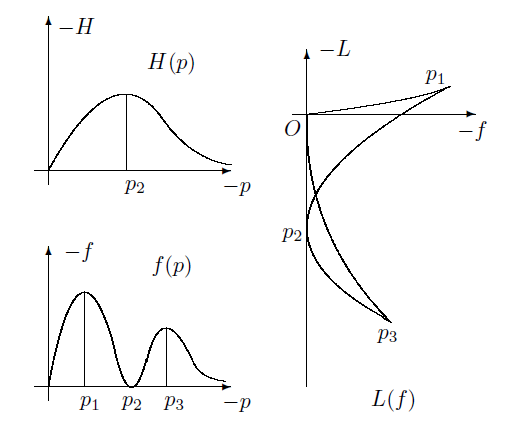
Figure 2: Example of branching $L(f)$ in an electric solution

The Hamiltonian framework might seem to be not worse than the Lagrangian one, even though the latter directly follows from the least action principle. However, it turns out[8] that at $p=p^{*}$ the electromagnetic field is singular: the effective metric [43, 44] in which NED photons move along null geodesics, is singular at extrema of $f(p)$, photons are there infinitely blueshifted [8, 44] and can create a curvature singularity by back reaction on the metric. Thus any regular electric solution not only fails to correspond to a fixed Lagrangian $L(f)$ but has other important undesired features.

We conclude that each choice of $A(r)$ gives rise to both electric and magnetic solutions related by FP duality. In these solutions the NED theories are different, and if $A(r)$ describes a geometry with a regular center and a RN asymptotic at large $r$, only the magnetic solution is really regular.

3.2 Dyonic configurations

Let us now assume that both $q_{e}$ and $q_{m}$ are nonzero. The difficulty in finding the solutions is that now $f(r)$ (or alternatively $p(r)$) is not known explicitly. Using, for definiteness, the Lagrangian formulation of the theory, we have

$$f(r)=\frac{2}{r^{4}}\biggl{(}q_{m}^{2}-\frac{q_{e}^{2}}{L_{f}^{2}}\biggr{)}.$$ (18)

Comparing the expressions for ${\cal E}(r)$ from (2) and (16), we can write ($M^{\prime}\equiv dM/dr$)

$${{\displaystyle\frac{1}{2}}}L(f)+\frac{2q_{e}^{2}}{L_{f}r^{4}}=\frac{2M^{\prime}(r)}{r^{2}}={\cal E}(r).$$ (19)

Let us specify the theory by choosing $L(f)$. Then Eq. (18) can be considered as either (A) an equation (in general, transcendental) for the function $f(r)$ or (B) an expression of $r$ as a function of $f$.

In case A, if $f(r)$ can be found explicitly, integration of Eq. (19) (equivalent to (16)) gives the metric function $A(r)$, and this completes the solution.

Scheme B leads to a solution in quadratures in terms of $f$ which can be chosen as a new radial coordinate. Indeed, assuming that $L(f)$ and $r(f)$ are known and monotonic, so that $L_{f}\neq 0$ and $r_{f}\neq 0$, Eq. (19) can be rewritten as

$$M_{f}=\frac{r^{2}r_{f}}{2}\biggl{[}\frac{L}{2}+\frac{q_{e}^{2}}{L_{f}r^{4}}\biggr{]}$$ (20)

(the subscript $f$ denotes $d/df$). Since the r.h.s. of (20) is known, it is straightforward to find $A(r)$ and to pass on to the coordinate $f$ in the metric. This gives us a general scheme of finding dyonic solutions under the above conditions.

Consider two examples using scheme A. The first example is used to verify the method: the Maxwell theory, $L=f$, $L_{f}=1$. Then from Eq. (19) we obtain $2M^{\prime}=(q_{e}^{2}+q_{m}^{2})/r^{2}$, whence $2M(r)=2m-(q_{e}^{2}+q_{m}^{2})/r$ and

$$A(r)=1-\frac{2m}{r}+\frac{q_{e}^{2}+q_{m}^{2}}{r^{2}},\ \ \ m={\rm const},$$ (21)

that is, the dyonic RN solution, as should be the case.

In the second example we assume that Eq. (18) is linear with respect to $f$, which unambiguously leads to the truncated Born-Infeld Lagrangian,

$$L(f)=b^{2}\big{(}-1+\sqrt{1+2f/b^{2}}\big{)},\ \ \ b={\rm const}$$ (22)

(the full Born-Infeld Lagrangian would also contain the invariant $(^{*}F_{\mu\nu}F^{\mu\nu})^{2}$).

Indeed, Eq. (18) is linear in $f$ only if $L_{f}^{-2}=c_{1}f+c_{2}$, $c_{1,2}={\rm const}$. Integration gives $L=L_{0}+(2/c_{1})\sqrt{c_{1}f+c_{2}}$. For a Maxwell behavior ($L{\approx}f$) at small $f$ we put $c_{2}=1$, $L_{0}=-2/c_{1}$. Denoting $2/c_{1}=b^{2}$, we arrive at Eq. (22), and

$${}f(r)=\frac{2b^{2}(q_{m}^{2}-q_{e}^{2})}{4q_{e}^{2}+b^{2}r^{4}},\hskip 28.45274pt{\cal E}(r)=-\frac{b^{2}}{2}+\biggl{(}\frac{b^{2}}{2}+\frac{2q_{e}^{2}}{r^{4}}\biggr{)}S(r),$$ (23)

where

$$S(r)=\sqrt{1+\frac{2f}{b^{2}}}=\sqrt{\frac{4q_{m}^{2}+b^{2}r^{4}}{4q_{e}^{2}+b^{2}r^{4}}}.$$

The simplest solution corresponds to the special case of a self-dual electromagnetic field, $q_{e}^{2}=q_{m}^{2}$, whence $S(r)=1$, $f=0$, and $L_{f}=1$ as in the Maxwell theory. This leads to ${\cal E}=2q_{e}^{2}/r^{4}$ and the dyonic RN metric with $A(r)$ given by (21).

In the general case $q_{e}^{2}\neq q_{m}^{2}$, $M(r)$ and $A(r)$ are expressed in terms of the Appell hypergeometric function $F_{1}$:

$$2M(r) = 2m+\frac{12q_{e}^{2}S(r)+b^{2}r^{4}(1+3S(r))}{6r}$$ (24)

$$\ +\frac{b^{2}r^{3}}{42|q_{e}q_{m}|}\biggl{[}14(q_{e}^{2}+q_{m}^{2})F_{1}\biggl{(}\frac{3}{4},{{\displaystyle\frac{1}{2}}},{{\displaystyle\frac{1}{2}}},\frac{7}{4},-\frac{b^{2}r^{4}}{4q_{e}^{2}},-\frac{b^{2}r^{4}}{4q_{m}^{2}}\biggr{)}$$

$$\hskip 28.45274pt+3b^{2}r^{4}F_{1}\biggl{(}\frac{7}{4},{{\displaystyle\frac{1}{2}}},{{\displaystyle\frac{1}{2}}},\frac{11}{4},-\frac{b^{2}r^{4}}{4q_{e}^{2}},-\frac{b^{2}r^{4}}{4q_{m}^{2}}\biggr{)}\biggr{]},$$

where $m={\rm const}$, and $A(r)=1-2M(r)/r$.

Some features of the solution should be noticed. As expected, the center $r=0$ is singular in accord with the above no-go theorem. At large $r$ the quantities $f_{e}$. $f_{m}$ and the energy density ${\cal E}$ decay as $r^{-4}$, and the solution is asymptotically flat and approximately RN. At small $r$, $f(r)$ tends to a finite limit while ${\cal E}\approx 2|q_{e}q_{m}|/r^{4}$. In a pure electric solution we also have ${\cal E}\sim r^{-4}$, while in a pure magnetic one ${\cal E}\sim r^{-2}$. Thus all solutions are singular at the center $r=0$, but the in the pure magnetic solution the singularity (existing since the function (22) does not tend to a finite limit as $f\to\infty$) is milder.

4 Dynamic wormholes

Apart from BH and solitonic configurations with a regular center, there can exist regular objects having no center at all, namely, wormholes and some classes of regular BHs, including the so-called black universes (BHs in which beyond the event horizon, instead of a singularity, there is an expanding universe), see, e.g., Refs. bu1–bu3. In the static case all of them require violation of the Null Energy Condition that states $T^{t}_{t}-T^{x}_{x}\geq 0$. Since for the SET (2) such a difference is zero, this condition (though marginally) is observed by NED, so static wormholes are manifestly impossible in the theory (1). However, as shown by Arellano and Lobo [19], wormhole solutions can be obtained if we consider evolving space-times. We will try to extend their finding, considering a more general class of time-dependent metrics.

4.1 Equations

In Ref. Arel-06 and the subsequent discussion [20, 21], the metric was chosen to be static times a time-dependent conformal factor. Let us assume a more general metric,

$$ds^{2}={\,\rm e}^{2\gamma(x)+2\nu(t)}dt^{2}-{\,\rm e}^{2\alpha(x)+2\eta(t)}dx^{2}-{\,\rm e}^{2\beta(x)+2\omega(t)}d\Omega^{2},$$ (25)

and NED as the matter source of gravity as given in (1). The function $\nu(t)$ can be absorbed by redefinition of $t$ and $\alpha(x)$ by redefinition of $x$, with the result

$$ds^{2}={\,\rm e}^{2\gamma(x)}dt^{2}-{\,\rm e}^{2\eta(t)}dx^{2}-{\,\rm e}^{2\beta(x)+2\omega(t)}d\Omega^{2}$$ (26)

that substantially simplifies the Einstein equations. For this metric the nonzero components of the Ricci tensor are

$${}R^{t}_{t}={\,\rm e}^{-2\gamma}[2\ddot{\omega}+\ddot{\eta}+2\dot{\omega}{}^{2}+\dot{\eta}{}^{2}]-{\,\rm e}^{-2\eta}[\gamma^{\prime\prime}+\gamma^{\prime}(2\beta^{\prime}+\gamma^{\prime})],$$ (27)

$${}R^{x}_{x}={\,\rm e}^{-2\gamma}[\ddot{\eta}+\dot{\eta}(2\dot{\omega}+\dot{\eta})]-{\,\rm e}^{-2\eta}[2\beta^{\prime\prime}+\gamma^{\prime\prime}+2\beta^{\prime}{}^{2}+\gamma^{\prime}{}^{2}],$$ (28)

$${}R^{\theta}_{\theta}=R^{\phi}_{\phi}={\,\rm e}^{-2\gamma}[\ddot{\omega}+\dot{\omega}(2\dot{\omega}+\dot{\eta})]-{\,\rm e}^{-2\eta}[\beta^{\prime\prime}+\beta^{\prime}(2\beta^{\prime}+\gamma^{\prime})],$$ (29)

$${}R_{tx}=2\dot{\omega}\beta^{\prime}-2\dot{\omega}\gamma^{\prime}-2\dot{\eta}\beta^{\prime}.$$ (30)

The electromagnetic field equations lead to the same relations (5) and (2) as in the static metric, where now $r={\,\rm e}^{\beta(x)+\omega(t)}$, preserving its geometric meaning of the spherical radius. As before, the $(xt)$ component of the SET is zero, and the corresponding Einstein equation $R_{xt}=0$ takes the form

$$\dot{\omega}(\beta^{\prime}-\gamma^{\prime})=\beta^{\prime}\dot{\eta},$$ (31)

where dots denote $\partial/dt$ and primes $\partial/\partial x$. Assuming $\beta^{\prime}\neq 0$, $\dot{\omega}\neq 0$ and dividing Eq. (31) by $\beta^{\prime}\dot{\omega}$, we separate the variables and, without loss of generality, obtain

$$\eta(t)=b\omega(t),\hskip 28.45274pt\gamma(x)=(1-b)\beta(x),$$ (32)

where $b$ is the separation constant. Next, since $T^{t}_{t}=T^{x}_{x}$, we have the equation $R^{t}_{t}=R^{x}_{x}$, where, excluding $\gamma$ and $\eta$ according to (32), we again separate the variables, obtaining

$${\,\rm e}^{2b\omega}[\ddot{\omega}+(1-b)\dot{\omega}{}^{2}]=-{\,\rm e}^{2(1-b)\beta}[\beta^{\prime\prime}+b\beta^{\prime}{}^{2}]=-k^{2},$$ (33)

with the separation constant $k^{2}{>\,}0$ assumed to be positive since we are seeking solutions with a minimum ($\beta^{\prime}{=}0,\beta^{\prime\prime}{>\,}0$) of the function $\beta(x)$, describing a throat in 3D spatial sections $t={\rm const}$.

Thus $\beta(x)$ and $\omega(t)$ are determined by the equations

$${}\beta^{\prime\prime}+b\beta^{\prime}{}^{2}=k^{2}{\,\rm e}^{2(b-1)\beta},$$ (34)

$${}\ddot{\omega}+(1-b)\dot{\omega}{}^{2}=-k^{2}{\,\rm e}^{-2b\omega},$$ (35)

whose first integrals are easily found. Specifically, for $b\neq 1/2$ we have

$$\beta^{\prime}{}^{2}=C_{1}{\,\rm e}^{-2b\beta}+\frac{k^{2}}{2b-1}{\,\rm e}^{2(b-1)\beta},\hskip 28.45274pt\dot{\omega}{}^{2}=C_{2}{\,\rm e}^{2(b-1)\omega}+\frac{k^{2}}{2b-1}{\,\rm e}^{-2b\omega},$$ (36)

and for $b=1/2$

$$\beta^{\prime}{}^{2}=(C_{3}+2k^{2}\beta){\,\rm e}^{-\beta},\hskip 28.45274pt\dot{\omega}{}^{2}=(C_{4}-2k^{2}\omega){\,\rm e}^{-\omega},$$ (37)

where $C_{1-4}$ are integration constants.

4.2 Geometry

Solutions to Eqs. (36) and (37) completely determine the metric under the ansatz (25) or (26) for any kind of matter whose SET satisfies the conditions $T^{t}_{t}=T^{x}_{x}$ and $T_{tx}=0$. As already mentioned, these conditions define the so-called Dymnikova vacuum [39, 40], for which any reference frame in radial motion is comoving.

In all cases under consideration, by construction, any 3D section $t={\rm const}$ of space-time contains a throat defined as a minimum of $\beta(x)$ and hence of $r={\,\rm e}^{\beta(x)+\omega(t)}$ at any given time instant, whereas the global features of these space-times depend on the constants involved.

Some immediate observations on the time dependence of $\omega$.follow directly from Eq. (35). Thus, a regular minimum of ${\,\rm e}^{\omega}$ (that is, a bounce in the time evolution of $r(x,t)$) is impossible since Eq. (35) leads to $\ddot{\omega}<0$ at points where $\dot{\omega}=0$ and ${\,\rm e}^{\omega}>0$. Next, a finite limit of ${\,\rm e}^{\omega}$ as $t\to\pm\infty$ is also impossible because at such a minimum the l.h.s. would be zero while the r.h.s. is finite. So the only possible way of regular evolution of ${\,\rm e}^{\omega}$ is to begin or end with ${\,\rm e}^{\omega}\to 0$ at infinite proper time, which is not completely excluded.

Further integration of Eqs. (36) for $b\neq 1/2$ leads in the general case to the hypergeometric function ${}_{2}F_{1}$:

$${}\pm t=\bigg{|}\frac{2b-1}{k^{2}}\bigg{|}^{1/2}\frac{{\,\rm e}^{(2-b)\omega}}{2-b}{}_{2}F_{1}\biggl{(}{{\displaystyle\frac{1}{2}}},1-\frac{b}{2},2-\frac{b}{2},\frac{2b-1}{k^{2}}C_{2}{\,\rm e}^{2\omega}\biggr{)},$$

$${}\pm x=\bigg{|}\frac{2b-1}{k^{2}}\bigg{|}^{1/2}\frac{{\,\rm e}^{(1+b)\beta}}{1+b}{}_{2}F_{1}\biggl{(}{{\displaystyle\frac{1}{2}}},\frac{1+b}{2},\frac{3+b}{2},\frac{2b-1}{k^{2}}C_{1}{\,\rm e}^{2\beta}\biggr{)},$$ (38)

while integration of Eq. (37) for $b=1/2$ involves the error function Erf:

$${}\pm t=\frac{\sqrt{\pi}}{k}{\,\rm e}^{-C_{4}/(4k^{2})}\biggl{[}-1+{\rm Erf}\,\bigg{(}\frac{\sqrt{C_{4}-2k^{2}\omega}}{2k}\bigg{)}\biggr{]},$$

$${}\pm x=\frac{\sqrt{\pi}}{k}{\,\rm e}^{C_{3}/(4k^{2})}\biggl{[}-1+{\rm Erf}\,\bigg{(}\frac{\sqrt{C_{3}+2k^{2}\omega}}{2k}\bigg{)}\biggr{]}.$$ (39)

Both solutions (4.2) and (4.2) are rather hard for further investigation, let us therefore restrict ourselves to some simple special cases.

Example 1: $b=1$. In this special case we obtain $\eta(t)\equiv\omega(t)$ and thus restore the isotropic nature of space-time evolution considered in Refs. Arel-06–Arel-09. The metric takes the form

$$ds^{2}=dt^{2}-{\,\rm e}^{2\omega(t)}\big{(}dx^{2}+{\,\rm e}^{2\beta(x)}d\Omega^{2}\big{)}.$$ (40)

Assuming $b=1$ in Eqs. (36) and (37), we obtain the following solutioon under a proper choice of the zero points of the coordinates $x$ and $t$:

$${}{\,\rm e}^{\beta}(x)=r_{0}\cosh(kx),\quad\ r_{0}={\rm const};\qquad{\,\rm e}^{\omega}=\left\{\begin{array}[]{ll}(k/h)\sinh(ht),&\ h>0,\\[5.0pt] {}kt,&\ h=0,\\[5.0pt] {}(k/h)\sin(ht),&\ h<0,\end{array}\right.$$ (44)

where we have denoted $C_{2}=h^{2}\mathop{\rm sign}\nolimits h$. It can be directly verified that this solution coincides with the one considered in Refs. Arel-06–Arel-09, but in another, more preferable parametrization: in (44) the coordinate $t$ is proper time, and $x$ is proportional to the proper distance at any fixed time $t$. Thus the spatial sections are evidently of wormhole nature but not asymptotically flat (the latter would require $r\propto|x|$ at large $|x|$ whereas here $r\propto{\,\rm e}^{k|x|}$), while the time evolution is different for different $h$: at $h\geq 0$ it is semi-infinite, and at $h<0$ it occupies a finite period between two zeros of $\sin(ht)$. The zeros of ${\,\rm e}^{\omega}(t)$ correspond to big-bang type singularities.

Example 2: $b=0$. In this case there is no expansion or contraction in the radial direction, and the coordinate $x$ is the true radial length in the reference frame used. The metric has the form

$$ds^{2}=e^{2\beta(x)}dt^{2}-dx^{2}-e^{2\omega(t)+2\beta(x)}d\Omega^{2}.$$ (45)

Integration of Eqs. (36) gives:

$${\,\rm e}^{\beta}=\frac{k}{m}\cosh(mx),\qquad{\,\rm e}^{\omega}=\frac{n}{k}\sin(kt),\qquad k,m,n>0,$$ (46)

where we have denoted $C_{1}=m^{2}$, $C_{2}=n^{2}$ (both $C_{1}$ and $C_{2}$ should be positive for Eqs. (36) to be meaningful). The properties of this solution are to a large extent the same as those of the branch $h<0$ in Example 1, but a significant difference is the emergence of $g_{tt}=e^{2\beta(x)}$ that grows together with $r^{2}(x)$ at large $|x|$ somewhat similarly to the static anti-de Sitter metric.

Example 3: $b\not\in\{0,1/2,1\},C_{1}=C_{2}=0$. In this case Eqs. (36) are also easily integrated in elementary functions, but the first equation implies $\beta^{\prime 2}>0$, that is, no throats are possible in the spacial sections of this space-time. Since we are seeking wormhole solutions, we do not consider this case any more.

It is clear that at the throat in all cases the gradient of the spherical radius $r(x,t)$ treated as a scalar function in 2D space-time parametrized by $t$ and $x$ is timelike since $r^{\prime}=0$ while $\dot{r}\neq 0$. Thus at least a certain neighborhood of the throat is a so-called T-region, i.e., a region where $r(x,t)$ may be chosen as a temporal coordinate (as happens, e.g., inside a Schwarzschild horizon), and the geometry is thus cosmological in nature, resembling Kantowski-Sachs spherically symmetric cosmologies [49, 40]. Does it mean that a T-region covers the whole space-time? An answer apparently depends on the parameters involved. For example, for the solution (44) we have

$$\partial^{\alpha}r\partial_{\alpha}r=r_{0}^{2}\cosh^{2}(kx)\biggl{[}{\,\rm e}^{2\omega(t)}\,h^{2}\mathop{\rm sign}\nolimits h+\frac{k^{2}}{\cosh^{2}(kx)}\biggr{]}.$$ (47)

Thus in models with $h\geq 0$ we have $\partial^{\alpha}r\partial_{\alpha}r>0$, i.e., the gradient of $r$ is timelike in the whole space-time, it is a global T-region. On the contrary, in the case $h<0$ we have $\partial^{\alpha}r\partial_{\alpha}r=0$ on the surfaces $x=\pm x_{h}(t)$ (apparent horizons) defined by the relation $\sin^{2}(ht)=1/\cosh^{2}(kx)$, and there are R-regions at $|x|>|x_{h}(t)|$, in this sense the space-time is of black hole type.

4.3 Electromagnetic fields

Let us return to NED as the matter source of gravity. It is easy to notice that the suitable form of $L(f)$ depends on the values of $q_{e}$ and $q_{m}$. As follows from the expressions (2), the magnetic field ${\bf B}$ is regular at all finite $r$, while the electric field ${\bf E}$ can tend to infinity not only where $r\to 0$ but also at zeros of the derivative $L_{f}$ if any.

Pure magnetic solutions are the simplest, just as in the static case. Indeed, assuming $q_{e}=0$ and $q_{m}\neq 0$, we have $L(f)=2R^{\theta}_{\theta}$, and using (36) and (37), it is easy to verify that $R^{\theta}_{\theta}$ is expressed in terms of $r={\,\rm e}^{\beta+\omega}$ rather than separately in terms of $\beta(x)$ and $\omega(t)$:

$${}R^{\theta}_{\theta}=r^{-2}+(2b{-}3)C_{1}r^{-2b}+(2b{-}1)C_{2}r^{2(b-1)},\qquad b\neq 1/2,$$ (48)

$${}R^{\theta}_{\theta}=r^{-2}+r^{-1}[2(C_{4}-C_{3})+k^{2}\ln(r/r_{0})],\qquad b=1/2,$$ (49)

where $r_{0}$ is an arbitrary constant introduced for dimensional considerations, and its choice can is related to the arbitrariness of the constant $C_{4}-C_{3}$. Since $f=2q_{m}^{2}/r^{4}$, it is straightforward to find $L(f)$ by substituting $r=(af)^{-1/4}$, where $a=(2q_{m}^{2})^{-1}$:

$${}{{\displaystyle\frac{1}{2}}}L(f)=(af)^{1/2}+(2b{-}1)C_{2}(af)^{(1-b)/2}+(2b{-}3)C_{1}(af)^{b/2},\qquad b\neq 1/2,$$ (50)

$${}{{\displaystyle\frac{1}{2}}}L(f)=(af)^{1/2}+(af)^{1/4}[2(C_{4}-C_{3})+k^{2}\ln(f/f_{0})],\qquad b=1/2,$$ (51)

where $f_{0}$ is introduced similarly to $r_{0}$. It is the full set of NED Lagrangians that lead to magnetic solutions of GR/NED equations with the metric (26). We see that none of these $L(f)$ possess a Maxwell behavior at small $f$.

The corresponding electric solutions with the same metric pertain to other versions of NED, as follows from the FP duality described in Section 2. For the same metric (26) we now have $H=-2R^{\theta}_{\theta}$, which, as we saw, is a function of $r$, and since now $p=-2q_{e}^{2}/r^{4}$, we know the function $H(p)$ which is the same as $-L(f)$ in (50) and (51), where $a$ should be replaced with $c=-1/(2q_{e}^{2})$, and $f$ with $p$, so that

$${}-{{\displaystyle\frac{1}{2}}}H(p)=(cp)^{1/2}+(2b{-}1)C_{2}(cp)^{(1-b)/2}+(2b{-}3)C_{1}(cp)^{b/2},\qquad b\neq 1/2,$$ (52)

$${}-{{\displaystyle\frac{1}{2}}}H(p)=(cp)^{1/2}+(cp)^{1/4}[2(C_{4}-C_{3})+k^{2}\ln(p/p_{0})],\qquad b=1/2,$$ (53)

Then, both $L$ and $f$ can in principle be found according to (14) as well as the function $f(p)$, and, as in the static case, there should be as many different Lagrangians $L(f)$ in different parts of space-time as is the number of monotonicity ranges of $f(p)$. From (52) and (53) we can find $L$ in terms of $p$ (either as $L=2pH_{p}-H$ or from the Einstein equations giving, for electric solutions, $L=2R^{t}_{t}$), so that

$${}{{\displaystyle\frac{1}{2}}}L=C_{1}(b-1)(3-2b)r^{-2b}+C_{2}b(2b+1)r^{2(b-1)},\qquad b\neq 1/2,$$ (54)

$${}{{\displaystyle\frac{1}{2}}}L=\frac{1}{r}\Big{[}-3+C_{4}-C_{3}+2k^{2}\ln(r/r_{0})\Big{]},\qquad b=1/2.$$ (55)

and substituting $r=(cp)^{-1/4}$. The function $f(p)$ is also easily found since $f(p)=pH_{p}^{2}$, and $H(p)$ is known. However, it is in general hard to find $L(f)$ and $p(f)$ in an explicit form since finding the inverse of $f(p)$ requires solving a transcendental equation.

Let us look what happens in the above two simple examples, $b=1$ and $b=0$.

Example 1: $b=1$, with the metric (40), (44). For magnetic wormholes, Eq. (50) gives

$$L(f)=2(1-C_{1})(af)^{1/2}+2C_{2},$$ (56)

a Lagrangian of the form previously used in a number of studies, see, e.g., Refs. hendi-13, guen-14 and references therein. For magnetic wormholes supported by NED in 2+1 dimensions such a Lagrangian was considered in Ref. mazh-17.

For electric wormholes with the same metric the function $-H(p)$ has the form (56) with the substitution $af\mapsto cp$, see above. Assuming $C_{1}\neq 1$, we obtain $H_{p}\sim|p|^{-1/2}\sim r^{2}$, hence $f=pH_{p}^{2}={\rm const}$. This strange result still does not immediately lead to a contradiction because by Eq. (54) we have also $L=3C_{2}={\rm const}$. So this solution corresponds to a constant $f=F_{\mu\nu}F^{\mu\nu}$ at which the function $L(f)$ has a certain particular value, but at other values of $f$ the function $L(f)$ is not defined. However, since $L_{f}=1/H_{p}\sim 1/r^{2}$, the derivative $L_{f}$ has different values at different space-time points, and since $f$ is fixed, it is inconsistent with any well-defined function $L(f)$. This makes the Lagrangian formulation of the theory ill-defined for this electric solution.

Example 2: $b=0$, with the metric (45), (46). For magnetic wormholes, Eq. (50) gives

$$L(f)=2(1-C_{2})(af)^{1/2}-3C_{1},$$ (57)

in full similarity with (56), up to the choice of the integration constants $C_{1},C_{2}$. So this is one more kind of magnetic wormhole geometry supported by NED with such Lagrangians. As to electric wormholes with the same geometry, the function $L(f)$ for them is again ill-defined for the same reasons as in Example 1.

For dyonic solutions with the same metrics, the problem of finding suitable NED formulations is more difficult and will not be considered here.

5 Concluding remarks

1. We have recalled the problem of obtaining regular static, spherically symmetric black hole solutions in GR with NED as a source of gravity and stressed the fundamental distinction between electric and magnetic fields, connected with the absence of the familiar duality inherent to the Maxwell electrodynamics. In the latter, knowing, for example, a magnetic field, it is straightforward to obtain any mixture of electric and magnetic fields by duality rotations. Unlike that, in the NED framework, FP duality connects only pure electric and pure magnetic configurations with the same metric but sourced by different versions of NED. It also happens that only pure magnetic solutions lead to completely regular configurations flat at infinity since their electric counterparts exhibit undesired features at some intermediate radii. Next, it turns out that finding dyonic configurations in NED/GR is quite a nontrivial problem, and only some special examples of such solutions are known.

2. In our search for evolving wormhole solutions, we have obtained a new family of geometries, which are in general not conformally static, except for a special case where they reduce to the known solutions of Ref. Arel-06. Under the metric ansatz (26), these geometries represent the general solution of GR for Dymnikova’s vacuum, defined by its transformation properties in the ($x^{0},x^{1}$) 2D subspace, similar to the properties of the cosmological constant in the whole 4D space-time. A general feature of these geometries is the existence of a throat in their spatial sections. However, their time evolution in general contains cosmological-type singularities. It has been shown that they can neither have a bounce of $r(x,t)$ nor begin or end with its finite value as $t\to-\infty$. It is not excluded that they have a “remote singularity”, that is, a zero value of $r$ as $t\to\pm\infty$, but even this opportunity may be ruled out in a future study. The existence of singularities at finite times is confirmed by examples given by Eqs. (44) and (46).

3. All that was independent of the particular choice of Dymnikova’s vacuum. If we apply NED for its implementation, it is rather easy to obtain these solutions with pure magnetic fields, but the choice of suitable NED Lagrangians is quite narrow and is expressed in Eqs. (50) and (51). None of these Lagrangians have a Maxwell weak field limit.

4. We have extended the FP duality, previously formulated for static systems, to time-dependent ones and used it for comparison between the electric and magnetic evolving wormhole solutions. The electric solutions are obtained in the “Hamiltonian” formulation of NED in the same way as magnetic ones in its Lagrangian formulation. However, it is in general hard to obtain a Lagrangian $L(f)$ for a given electric solution due to a necessity to deal with transcendental equations. Moreover, in particular examples the Lagrangian formulation is ill-defined for electric solutions.

To conclude, the NED/GR system exhibits some unusual and unexpected features and deserves a further study and discussion.

Acknowledgments

I thank Milena Skvortsova, Sergei Bolokhov and Sergei Rubin for helpful discussions. The work was partly performed within the framework of the Center FRPP supported by MEPhI Academic Excellence Project (contract No. 02.a03.21.0005, 27.08.2013). The work was also funded by the RUDN University Program 5-100 and by RFBR grant 16-02-00602.

References

- [1] M. Born and L. Infeld, Foundations of the new field theory, Proc. R. Soc. Lond. 144, 425 (1934).
- [2] W. Heisenberg and H. Euler, Folgerungen aus der Diracschen Theorie des Positrons, Z. Phys. 98, 714 (1936).
- [3] J. Plebanski, Non-Linear Electrodynamics — A Study (C.I.E.A. del I.P.N., Mexico City, 1966).
- [4] N. Seiberg and E. Witten, String theory and noncommutative geometry, J. High Energy Phys. 09, 032 (1999); hep-th/9908142.
- [5] A. A. Tseytlin, Born-Infeld action, supersymmetry and string theory, hep-th/9908105.
- [6] R. Pellicer and R. J. Torrence, Nonlinear electrodynamics and general relativity, J. Math. Phys. 10, 17+18 (1969).
-
[7]
K. A. Bronnikov and G. N. Shikin,
On the Reissner-Nordström problem with a nonlinear electromagnetic field,
in Classical and Quantum Theory of Gravity (Trudy IF AN BSSR, Minsk, 1976),
p. 88 (in Russian);
K. A. Bronnikov, V. N. Melnikov, G. N. Shikin, and K. P. Staniukovich, Scalar, electromagnetic, and gravitational fields interaction: particlelike solutions, Ann. Phys. (N.Y.) 118, 84 (1979). - [8] K. A. Bronnikov, Regular magnetic black holes and monopoles from nonlinear electrodynamics, Phys. Rev. D 63, 044005 (2001); gr-qc/0006014.
- [9] K. A. Bronnikov, Comment on ‘Regular black hole in general relativity coupled to nonlinear electrodynamics’ , Phys. Rev. Lett. 85, 4641 (2000).
- [10] K. A. Bronnikov, Dyonic configurations in nonlinear electrodynamics coupled to general relativity, Grav. Cosmol. 23, 343 (2017); arXiv: 1708.08125.
- [11] A. Burinskii and S. R. Hildebrandt, New type of regular black holes and particlelike solutions from nonlinear electrodynamics, Phys. Rev. D 65, 104017 (2002); hep-th/0202066 .
- [12] J. Matyjasek, D. Tryniecki, and M. Klimek, Regular black holes in an asymptotically de Sitter universe, Mod. Phys. Lett. A 23, 3377 (2009); arXiv: 0809.2275.
- [13] N. Bretón, Smarr’s formula for black holes with non-linear electrodynamics, Gen. Rel. Grav. 37, 643 (2005); gr-qc/0405116.
- [14] S. I. Kruglov, Asymptotic Reissner-Nordström solution within nonlinear electrodynamics, Phys. Rev. D 94, 044026 (2016); arXiv: 1608.04275.
- [15] Zhong-Ying Fan and Xiaobao Wang, Construction of regular black holes in general relativity, Phys. Rev. D 94, 124027 (2016); arXiv: 1610.02636.
- [16] K. A. Bronnikov, G. N. Shikin, and E. N. Sibileva, Self-gravitating stringlike configurations from nonlinear electodynamics, Grav. Cosmol. 9, 169 (2003); gr-qc/0308002.
- [17] C. Bambi and L. Modesto, Rotating regular black holes, Phys. Lett. B 721, 329 (2013); arXiv: 1302.6075.
- [18] I. Dymnikova and E. Galaktionov, Regular rotating electrically charged black holes and solitons in nonlinear electrodynamics minimally coupled to gravity, Class. Quantum Grav. 32, 165015 (2015); arXiv: 1510.01353.
- [19] A. V. B. Arellano and F. S. N. Lobo, Evolving wormhole geometries within nonlinear electrodynamics, Class. Quantum Grav. 23, 5811 (2006); gr-qc/0608003.
- [20] Ch. G. Boehmer, T. Harko, and F. S. N. Lobo, Conformally symmetric traversable wormholes, Phys. Rev. D 76, 084014 (2007); arXiv: 0708.1537.
- [21] A. V. B. Arellano, N. Bretón, and R Garcia-Salcedo, Some properties of evolving wormhole geometries within nonlinear electrodynamics, Gen. Rel. Grav. 41, 2561 (2009); arXiv: 0804.3944.
- [22] C. Moreno and O. Sarbach, Stability properties of black holes in self-gravitating nonlinear electrodynamics, Phys. Rev. D 67, 024028 (2003); gr-qc/0208090.
- [23] N. Bretón, Stability of nonlinear magnetic black holes, Phys. Rev. D 72, 044015 (2005); hep-th/0502217.
- [24] Jin Li, Kai Lin and Nan Yang, Nonlinear electromagnetic quasinormal modes and Hawking radiation of a regular black hole with magnetic charge, Eur. Phys. J. C 75, 131 (2015); arXiv: 1409.5988.
- [25] W. Berej and J. Matyjasek, Vacuum polarization in the spacetime of charged nonlinear black hole, Phys. Rev. D 66, 024022 (2002); gr-qc/0204031.
- [26] J. Matyjasek, P. Sadurski, and D. Tryniecki, Inside the degenerate horizons of regular black holes, Phys. Rev. D 87, 124025 (2013); arXiv: 1304.6347.
- [27] M. Visser, Lorentzian Wormholes: From Einstein to Hawking (American Institute of Physics, New York, 1995)
- [28] F. S. N. Lobo, Exotic solutions in General Relativity: Traversable wormholes and warp drive spacetimes. In: Classical and Quantum Gravity Research, p. 1-78 (Nova Sci. Pub., 2008); ArXiv: 0710.4474.
- [29] K A. Bronnikov and S. G. Rubin, Black Holes, Cosmology, and Extra Dimensions (World Scientific, 2012).
- [30] F. S. N. Lobo (Editor). Wormholes, Warp Drives and Energy Conditions (Springer, 2017).
- [31] M .S. Morris and K. S. Thorne, Wormholes in spacetime and their use for interstellar travel: A tool for teaching general relativity. Am. J. Phys. 56, 395 (1988).
- [32] K. A. Bronnikov, Scalar-tensor theory and scalar charge. Acta Phys. Pol. B 4, 251 (1973).
- [33] H. Ellis, Ether flow through a drainhole — a particle model in general relativity. J. Math. Phys. 14, 104 (1973).
- [34] K. A. Bronnikov and A. M. Galiakhmetov, Wormholes and black universes without phantom fields in Einstein-Cartan theory. Phys. Rev. D 94, 124006 (2016); arXiv: 1607.07791.
- [35] G. Dotti, J. Oliva, and R. Troncoso, Static wormhole solution for higher-dimensional gravity in vacuum. Phys. Rev. D 75, 024002 (2007); hep-th/0607062.
- [36] T. Harko, F.S.N. Lobo, M.K. Mak, and S.V. Sushkov, Gravitationally modified wormholes without exotic matter, Phys. Rev. D 87, 067504 (2013); arXiv: 1301.6878.
- [37] K. A. Bronnikov and S.-W. Kim, Possible wormholes in a brane world. Phys. Rev. D 67, 064027 (2003), gr-qc/0212112.
- [38] K. A. Bronnikov and M. V. Skvortsova, Wormholes leading to extra dimensions. Grav. Cosmol. 22, 316 (2016); arXiv: 1608,04974.
- [39] I.G. Dymnikova, Vacuum nonsingular black hole. Gen. Rel. Grav. 24, 235 (1992).
- [40] K. A. Bronnikov, S.-W. Kim and M. V. Skvortsova, The Birkhoff theorem and string clouds, Class. Quantum Grav. 33, 195006 (2016); arXiv: 1604.04905.
- [41] I. H. Salazar, A. Garcia and J. Plebanski, Duality rotations and type D solutions to Einstein equations with nonlinear electromagnetic sources. J. Math. Phys. 28, 2171 (1987).
- [42] L. Balart and E. C. Vagenas, Regular black hole metrics and the weak energy condition Phys. Lett. B 730, 14 (2014); arXiv: 1401.2136.
- [43] M. Novello, V. A. de Lorenci, J. M. Salim, and R. Klippert, Geometrical aspects of light propagation in nonlinear electrodynamics, Phys. Rev. D 61, 045001 (2000).
- [44] M. Novello, S. E. Perez Bergliaffa, and J. M. Salim, Singularities in General Relativity coupled to nonlinear electrodynamics, Class. Quantum Grav. 17, 3821 (2000); gr-qc/0003052.
- [45] E. Ayon-Beato and A. Garcia, New regular black hole solution from nonlinear electrodynamics, Phys. Lett. B 464, 25 (1999)
- [46] K. A. Bronnikov and J. C. Fabris, Regular phantom black holes, Phys. Rev. Lett. 96, 251101 (2006); gr-qc/0511109.
- [47] K. A. Bronnikov, V. N. Melnikov and H. Dehnen, Regular black holes and black universes, Gen. Rel. Grav. 39, 973–987 (2007); gr-qc/0611022.
- [48] S. V. Bolokhov, K. A. Bronnikov, and M. V. Skvortsova, Magnetic black universes and wormholes with a phantom scalar, Class. Quantum Grav. 29, 245006 (2012); arXiv: 1208.4619.
- [49] V. P. Frolov an I. D. Novikov, Black Hole Physics: Basic Concepts and New Developments (Springer, 1998).
- [50] S. H. Hendi and A. Sheykhi, Charged rotating black string in gravitating nonlinear electromagnetic fields, Phys. Rev. D 88, 044044 (2013); arXiv: 1405.6998.
- [51] M. Vasihoun and E. Guendelman, Gravitational and topological effects on confinement dynamics. arXiv: 1406.0203.
- [52] S. Habib Mazharimousavi, Z. Amirabi, M. Halilsoy, Magnetic Morris-Thorne wormhole in 2+1-dimensions, Gen. Rel. Grav. 48, 143 (2016); arXiv: 1703.05316.