The Sloan Lens ACS Survey. XIII. Discovery of 40 New Galaxy-Scale Strong Lenses*

Abstract

We present the full sample of 118 galaxy-scale strong-lens candidates in the Sloan Lens ACS (SLACS) Survey for the Masses (S4TM) Survey, which are spectroscopically selected from the final data release of the Sloan Digital Sky Survey. Follow-up Hubble Space Telescope (HST) imaging observations confirm that 40 candidates are definite strong lenses with multiple lensed images. The foreground-lens galaxies are found to be early-type galaxies (ETGs) at redshifts 0.06–0.44, and background sources are emission-line galaxies at redshifts 0.22–1.29. As an extension of the SLACS Survey, the S4TM Survey is the first attempt to preferentially search for strong-lens systems with relatively lower lens masses than those in the pre-existing strong-lens samples. By fitting HST data with a singular isothermal ellipsoid model, we find that the total projected mass within the Einstein radius of the S4TM strong-lens sample ranges from $3\times 10^{10}M_{\odot}$ to $2\times 10^{11}M_{\odot}$. In Shu et al., we have derived the total stellar mass of the S4TM lenses to be $5\times 10^{10}M_{\odot}$ to $1\times 10^{12}M_{\odot}$. Both the total enclosed mass and stellar mass of the S4TM lenses are on average almost a factor of 2 smaller than those of the SLACS lenses, which also the represent typical mass scales of the current strong-lens samples. The extended mass coverage provided by the S4TM sample can enable a direct test, with the aid of strong lensing, for transitions in scaling relations, kinematic properties, mass structure, and dark-matter content trends of ETGs at intermediate-mass scales as noted in previous studies.

1. Introduction

Early-type galaxies (ETGs) are a group of galaxies that have regular ellipsoidal shapes, typically old stellar populations, and little ongoing star-formation activity. They are believed to be the end product of a hierarchical merging scenario of galaxy formation (e.g., Toomre & Toomre, 1972; White & Frenk, 1991; Kauffmann et al., 1993; Cole et al., 2000). Early works suggested that ETGs seemed to be a well-defined population by tightly following several empirical scaling relations (e.g., Faber & Jackson, 1976; Kormendy, 1977; Dressler et al., 1987; Djorgovski & Davis, 1987). However, as the sample became larger and more complete later on, clear transitions in several scaling relations, kinematic properties, and dark-matter content trends of ETGs were noted at two characteristic mass scales, $3\times 10^{10}M_{\odot}$ and $2\times 10^{11}M_{\odot}$ (e.g., Tremblay & Merritt, 1996; Graham & Guzmán, 2003; Kauffmann et al., 2003; Graham & Worley, 2008; Hyde & Bernardi, 2009; Skelton et al., 2009; Tortora et al., 2009; van der Wel et al., 2009; Bernardi et al., 2011a, b; Cappellari et al., 2013a, b; Montero-Dorta et al., 2016). This implies that that physical processes that regulate how ETGs form and evolve must have undergone similar transitions at these two mass scales.

Previous studies on the ETG transitions primarily used photometric data or stellar kinematics data inferred from spectra for ETG mass estimation, which are known to be model dependent and have weak constraining power on the dark-matter content. The strong gravitational lensing phenomenon, which is the appearance of multiple images of the same distant source due to the convergence of light caused by the gravitational field of an intervening object (denoted as the “lens”) as a prediction of Albert Einstein’s general relativity (GR; Einstein, 1916), provides a robust way of determining the total mass in the central region of the lens object (e.g., see a review article by Treu, 2010). Accurate mass measurements of ETG lens systems may provide new insights in understanding of such transitions, especially by combining low-, intermediate-, and high-mass ETG strong-lens samples.

Nevertheless, strong-lensing events are rare because it requires a close alignment among the observer, the lens, and the source. The probability of a lensing event occurring is characterized by the lensing cross section, which is the area on the source plane within which the source needs to be to produce at least two images. To the leading order, the lensing cross section is determined by the mass of the lens object, at least on the galaxy-scales that we are considering in this paper. Because of this, current galaxy-scale strong-lens searches are strongly biased toward massive ETGs for high success-rates. Over the past four decades, the number of strong-lens systems has accumulated to just a few hundred from dedicated photometric and/or spectroscopic surveys (e.g., Walsh et al., 1979; Muñoz et al., 1998; Kochanek et al., 2000; Browne et al., 2003; Ebeling et al., 2007; Bolton et al., 2008a; Faure et al., 2008; Treu et al., 2011; Brownstein et al., 2012; More et al., 2012; Inada et al., 2012; Sonnenfeld et al., 2013; Stark et al., 2013; Vieira et al., 2013; Pawase et al., 2014; More et al., 2016; Shu et al., 2016b; Negrello et al., 2017; Sonnenfeld et al., 2017). The typical stellar mass of the current galaxy-scale strong-lens sample is several times $10^{11}M_{\odot}$ (e.g., Auger et al., 2010; Faure et al., 2011; Brownstein et al., 2012; Sonnenfeld et al., 2013), beyond the above-mentioned characteristic mass scales. Note that this mass peak is primarily the result of the lensing cross section per lens, which is proportional to the mass to the second power, and galaxy mass function, which suggests that the number of ETGs typically increases with $1/M$ below the characteristic mass $M_{*}$ and declines exponentially beyond (e.g., Li & White, 2009; Yang et al., 2009; Ilbert et al., 2010; Baldry et al., 2012; Maraston et al., 2013; Davidzon et al., 2017). Clearly, a large sample of strong-lens systems containing low- and intermediate-mass ETG lenses is needed.

The Sloan Lens ACS (SLACS) Survey for the Masses (S4TM) Survey has been designed as an attempt to preferentially select relatively lower-mass strong-lens systems. To achieve that, we rely on the most prolific strong-lens selection technique ever developed, the one presented in Bolton et al. (2004). This technique has lead to several major strong-lens surveys including the Sloan Lens ACS Survey (SLACS; Bolton et al., 2008a; Auger et al., 2009), the Sloan WFC Edge-on Late-type Lens Survey (SWELLS; Treu et al., 2011; Brewer et al., 2012), the BOSS Emission-Line Lens Survey (BELLS; Brownstein et al., 2012), and the BELLS for GAlaxy-Ly$\alpha$ EmitteR sYstems survey (BELLS GALLERY; Shu et al., 2016b). From Hubble Space Telescope (HST) follow-up imaging observations, we have already confirmed nearly 150 strong-lens systems in total (85 in SLACS, 20 in SWELLS, 25 in BELLS, and 17 in BELLS GALLERY). However, previously, candidates with the highest predicted lensing cross sections (essentially largest lens masses) were prioritized in these HST observations. In the S4TM Survey, we try to extend the lens-mass coverage by targeting at candidates with relatively lower predicted lens mass at the cost of lowering the success rate. We will explain how we achieve this in Section 2.

This paper is organized as follows. Section 2 briefly describes how the lower-mass S4TM sample is selected. HST photometric data and strong-lensing analysis are provided in Sections 3 and 4. Section 5 presents the discussion followed by a summary in Section 6. Throughout the paper, we adopt a cosmological model with $\rm\Omega_{m}=0.274$, $\rm\Omega_{\Lambda}=0.726$ and $H_{0}\rm=70\,km\,s^{-1}\,Mpc^{-1}$ (WMAP7; Komatsu et al., 2011).

2. Sample Selection

As an extension of the SLACS survey, the S4TM survey selects strong-lens candidates spectroscopically from the galaxy-spectrum database provided by the seventh and final data release of the Sloan Digital Sky Survey (SDSS; Abazajian et al., 2009). The S4TM survey adopts the strong-lens selection technique that led to the successful discoveries of nearly 150 strong-lens systems (e.g., Bolton et al., 2008a; Auger et al., 2009; Treu et al., 2011; Brewer et al., 2012; Brownstein et al., 2012; Shu et al., 2016b; Marques-Chaves et al., 2017). The underlying principle is to select the candidate that shows multiple nebular emission lines in their spectra, collected by an optical fiber at a common redshift that is significantly higher than the candidate itself. Such a special configuration indicates that there are two objects at different redshifts within the same light cone, which is usually as narrow as 2–3 arcsec in diameter, and a lensing event is likely to happen. High-resolution follow-up imaging observations are then obtained to confirm the lensing nature of the system. More detailed descriptions on this technique can be found in Bolton et al. (2004), Brownstein et al. (2012), and Shu et al. (2016b).

After picking out strong-lens candidates with higher-redshift nebular emission lines from the SDSS DR7 database, we first perform a morphology cut by only retaining candidates with early-type morphology as determined from the SDSS images. Then we compute an approximate strong-lensing Einstein radius, $\theta_{\rm Ein}$, based on the foreground and background redshifts and SDSS measured central stellar velocity dispersion, assuming a singular isothermal sphere model. As shown in Bolton et al. (2008a), the SLACS lens confirmation rate is an increasing function of $\theta_{\rm Ein}$. We remove candidates with a predicted $\theta_{\rm Ein}$ smaller than 0$\farcs$5 because the confirmation rate drops rapidly to $\leqslant 10\%$ below this angular scale (Bolton et al., 2008a).

To specifically select lens galaxies to complement the SLACS survey in terms of lens-galaxy mass distribution, we rely on a dimensional mass variable defined as $M_{\rm dim}=G^{-1}\sigma^{2}R_{\rm eff}/2$ where $\sigma$ and $R_{\rm eff}$ are the SDSS measured stellar velocity dispersion and effective radius, respectively. Directly constructed from existing SDSS measurements, this dimensional mass, $M_{\rm dim}$, serves as a simple gauge of the lens galaxy mass, at least in a relative sense. Candidates with $M_{\rm dim}$ less than $10^{10.5}M_{\odot}$ ($\approx 3\times 10^{10}M_{\odot}$), a mass scale below which is sparsely populated by confirmed SLACS lenses, are included into the S4TM sample. An analysis of the SLACS sample further shows that the ratio of Einstein radius to effective radius of SLACS lenses is limited to a range from $\sim$0.4 to 1.0. This ratio is a useful scale in galaxy-scale strong lenses. Although mass measurements inferred from strong lensing are extremely accurate, they are limited to a physical radial aperture — the Einstein radius — that is determined by serendipitous cosmic geometry. In order to control effectively for systematic mass-aperture effects in the follow-up lensing and dynamical analyses, we would like to build up ensembles of strong-lens systems with a significant variation in the ratio of Einstein radius to optical effective radius for multiple fixed lens-galaxy mass ranges. Here the effective radius is a normalization factor. As a result, we also include in the S4TM sample candidates with similar dimensional masses as the SLACS lenses ($M_{\rm dim}>10^{10.5}M_{\odot}$), but with a predicted ratio of Einstein radius to effective radius $\theta_{\rm Ein}/R_{\rm eff}$ either less than 0.4 or greater than 1.0.

Eventually, the S4TM sample comprises 135 new galaxy–galaxy lens candidates. In combination with the SLACS sample, this lens ensemble covers nearly two decades in mass, with dense mapping of enclosed mass as a function of radius out to the effective radius and beyond.

3. HST Photometric Data

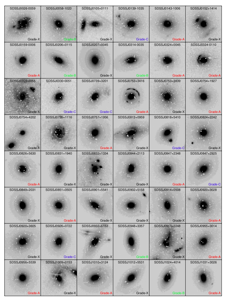
Figure 1.— Mosaic of the HST F814W-band images of the 118 S4TM strong-lens candidates. Images are $6^{\prime\prime}\times 6^{\prime\prime}$ with north up and east to the left. The SDSS name and lens grade are given for each system.

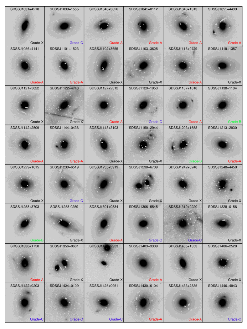
Figure 1.— Continued

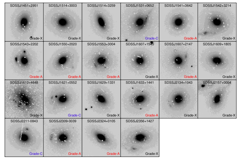
Figure 1.— Continued

HST imaging observations of the S4TM sample were carried out in the F814W-band with the Wide Field Channel (WFC) of the ACS camera under the Snapshot Program #12210 in Cycle 18 (PI: A. Bolton). Each candidate is designed to have a single exposure of 420 s during one HST visit. As of its completion, 118 visits are successfully observed, 2 visits are not usable (29, 35) because of guide star acquisition failure, and 15 visits are withdrawn. From now on, we will only focus on the 118 candidates with HST observations. The individual fully-calibrated, flat-fielded (FLT) files are downloaded from the HST archive and reduced by our custom-built tool, ACSPROC, presented in Brownstein et al. (2012). In order to be consistent with Bolton et al. (2008a), Brownstein et al. (2012), and especially Shu et al. (2015), which presents the first scientific results of the S4TM survey, we model the foreground lens-galaxy light with an elliptical radial B-spline model (Bolton et al., 2006a). Besides a B-spline model, we also fit the two-dimensional elliptical de Vaucouleurs model (de Vaucouleurs, 1948) to the foreground light to derive some standardized quantities such as the effective radius, axis ratio, and major-axis position angle. Such values along with other useful information determined from the SDSS spectroscopic data are presented in Table 1.

The B-spline-subtracted residual images are inspected by a group of authors (A.S.B., J.R.B., and Y.S.) to determine the lens morphology, multiplicity, and lens grade. As shown by the classification codes in Table 1, the majority of the 118 candidates contain single ETGs in the foreground. As mentioned in Shu et al. (2015), we identify 40 grade-A strong lenses with definite multiple lensed images, 8 grade-B systems with strong evidence of multiple images but insufficient signal-to-noise ratio for definite conclusion and/or modeling, and 18 grade-C systems clearly showing lensed images of the background galaxies but no clear counterimages. The remaining 52 candidates are classified as nonlenses (grade-X). Figure 1 shows the mosaic of the fully-reduced HST F814W-band images of all of the 118 systems. Target names and lens grades are given in each $6^{\prime\prime}\times 6^{\prime\prime}$ stamp. The small white blocks in each stamp correspond to the pixels masked due to cosmic rays, which we can not correct for based on single exposures. The success rate of finding grade-A lenses in the S4TM survey ($34\%$) is slightly lower than those in previous SLACS and BELLS surveys, which can reach about 50%. That could be related to the trade-off between success rate and lens-mass coverage in the S4TM Survey as discussed above. The average lens and source redshifts are 0.17 and 0.61, slightly lower than those of the SLACS lens sample (0.21 and 0.63, respectively). We note that none of the four galaxies in Table 1 with zero stellar velocity dispersions according to the SDSS reduction pipeline are grade-A.

4. Strong-lensing Analysis

Here we only report strong-lens modeling results for S4TM grade-A lenses, and refer the interested reader to Shu et al. (2015) for the results of the S4TM grade-C lenses and a combined analysis of grade-A and grade-C lenses in the SLACS and S4TM surveys.

Lens modeling is done with the custom-built tool lfit_gui first introduced in Shu et al. (2016b). There are three components in the lens model. The first component is the foreground-light model. For the same consistency reason, we adopt the B-spline fit as the model for the foreground-light distribution following Shu et al. (2015). Note that this foreground-subtraction strategy could introduce some systematic uncertainties in the lens and source parameters as discussed in Marshall et al. (2007) and Shu et al. (2016a, b). Following our previous works, we use the singular isothermal ellipsoid (SIE) profile to model the projected lens-mass distribution. Our singular isothermal ellipsoid (SIE) model has a two-dimensional surface mass–density profile following Kormann et al. (1994) as

$$\Sigma(x,y)=\Sigma_{\rm crit}\frac{\sqrt{q}}{2}\frac{b_{\rm SIE}}{\sqrt{x^{2}+q^{2}y^{2}}},$$ (1)

where $\Sigma_{\rm crit}$ is the critical density determined by the cosmological distances as

$$\Sigma_{\rm crit}=\frac{c^{2}}{4\pi G}\frac{d_{S}}{d_{L}d_{LS}},$$ (2)

and $d_{L}$, $d_{S}$, and $d_{LS}$ are the angular diameter distances from the observer to the lens, from the observer to the source, and between the lens and the source, respectively. We do not include any external shear in the lens model because it is a minor effect as quantified in Shu et al. (2015). The last component is the source model. As explained in Shu et al. (2016b), lfit_gui provides two types of source models. One is the parametric source model in which the source-light distribution is characterized by multiple elliptical Sérsic components. The other is the pixelized source model obtained from a direct inversion (e.g., Dye & Warren, 2005; Koopmans, 2005; Brewer & Lewis, 2006; Suyu et al., 2006; Vegetti & Koopmans, 2009; Nightingale & Dye, 2015). We start from a single Sérsic source component, and then generate a pixelized source model with all the lens model parameters fixed. Extra Sérsic components are added to match the pixelized source model. This procedure is done iteratively until the parametric source model and the pixelized source model are in reasonable agreement. The parameter optimization is done by minimizing a $\chi^{2}$ function using the Levenberg–Marquardt algorithm as implemented in the LMFIT package (Newville et al., 2014).

Table 1 Selected properties of the S4TM sample.

Target	Plate-MJD-Fiber	$z_{L}$	$z_{S}$	$\sigma_{\rm SDSS}$	$I_{\rm 814}$	$\Delta I_{\rm 814}$	$R_{\rm eff}$	$q$	P.A.	Classification
				(km s-1)	(mag)	(mag)	(arcsec)		(deg)
(1)	(2)	(3)	(4)	(5)	(6)	(7)	(8)	(9)	(10)	(11)
SDSSJ0026$-$0059	0391-51782-255	0.0924	0.9506	74 $\pm$ 19	16.87	0.04	4.92	0.65	125	E-S-X
SDSSJ0058$-$1020	0658-52146-191	0.3088	0.7741	295 $\pm$ 23	16.76	0.07	4.76	0.69	47	E-M-B
SDSSJ0105$+$0111	0670-52520-403	0.3584	1.1041	0 $\pm$ 0	18.99	0.04	0.83	0.58	89	E-S-X
SDSSJ0139$-$1035	0663-52145-201	0.2221	0.9745	209 $\pm$ 13	17.20	0.04	2.13	0.83	96	E-U-C
SDSSJ0143$-$1006	0664-52174-259	0.2210	1.1046	203 $\pm$ 17	16.85	0.05	3.24	0.78	82	E-S-A
SDSSJ0152$+$1414	0430-51877-473	0.1359	0.2920	121 $\pm$ 21	16.93	0.12	3.52	0.82	22	E-U-X
SDSSJ0159$-$0006	1555-53287-171	0.1584	0.7477	216 $\pm$ 18	17.47	0.05	1.58	0.91	139	E-S-A
SDSSJ0206$+$0115	0404-51877-530	0.1373	0.8749	187 $\pm$ 12	16.93	0.05	1.13	0.52	58	E-S-B
SDSSJ0207$+$0045	0404-51812-540	0.0419	1.1148	155 $\pm$ 4	14.80	0.05	3.10	0.83	13	E-S-X
SDSSJ0314$-$0035	0412-52258-030	0.1151	1.1501	172 $\pm$ 10	16.92	0.14	1.44	0.61	105	E-S-B
SDSSJ0324$+$0045	1629-52945-424	0.3210	0.9199	183 $\pm$ 19	18.23	0.22	1.67	0.84	90	E-S-A
SDSSJ0324$-$0110	1566-53003-246	0.4456	0.6239	310 $\pm$ 38	18.17	0.17	2.23	0.73	90	E-S-A
SDSSJ0329$-$0055	0713-52178-298	0.1062	0.6576	22 $\pm$ 75	16.84	0.23	10.00	0.87	21	L-S-X
SDSSJ0330$-$0051	0810-52672-304	0.3406	1.1334	194 $\pm$ 34	19.05	0.22	0.55	0.77	126	E-S-C
SDSSJ0739$+$3201	0541-51959-078	0.1860	0.6198	197 $\pm$ 6	17.10	0.09	1.00	0.66	138	E-S-C
SDSSJ0753$+$3416	0756-52577-482	0.1371	0.9628	208 $\pm$ 12	16.55	0.10	1.89	0.86	137	E-S-A
SDSSJ0753$+$3839	0544-52201-314	0.0408	1.2344	27 $\pm$ 25	17.10	0.08	3.37	0.86	26	E-S-X
SDSSJ0754$+$1927	1582-52939-627	0.1534	0.7401	193 $\pm$ 16	17.02	0.10	1.46	0.94	45	E-S-A
SDSSJ0754$+$4202	0434-51885-075	0.3692	1.0543	342 $\pm$ 71	17.19	0.08	4.63	0.56	133	E-S-X
SDSSJ0755$+$1116	2418-53794-354	0.1378	0.3448	0 $\pm$ 0	17.16	0.05	3.74	0.99	110	L-S-X
SDSSJ0757$+$1956	1922-53315-347	0.1206	0.8326	206 $\pm$ 11	15.82	0.09	3.67	0.91	154	E-S-A
SDSSJ0813$+$0959	2421-54153-171	0.1565	1.1851	195 $\pm$ 13	16.36	0.05	2.33	0.52	110	L-S-X
SDSSJ0818$+$5410	1782-53299-266	0.1163	0.3673	191 $\pm$ 12	16.90	0.10	1.06	0.68	130	E-S-C
SDSSJ0824$+$2242	1927-53321-521	0.2802	0.8457	321 $\pm$ 24	16.17	0.08	6.67	0.93	78	E-M-X
SDSSJ0826$+$5630	1783-53386-414	0.1318	1.2907	163 $\pm$ 8	16.27	0.11	1.64	0.87	51	E-S-A
SDSSJ0831$+$1940	2275-53709-362	0.0876	0.8805	155 $\pm$ 6	16.87	0.07	1.26	0.72	173	E-S-X
SDSSJ0832$+$1334	2425-54139-062	0.3968	0.7437	303 $\pm$ 24	16.98	0.11	3.97	0.74	1	E-M-X
SDSSJ0844$+$2113	2280-53680-388	0.1779	0.3091	246 $\pm$ 15	16.22	0.07	3.96	0.74	162	E-S-X
SDSSJ0847$+$2348	2085-53379-342	0.1551	0.5327	199 $\pm$ 16	17.00	0.06	1.54	0.94	90	E-S-A
SDSSJ0847$+$2925	1589-52972-252	0.1001	0.2390	228 $\pm$ 9	15.73	0.08	2.19	0.71	130	E-S-C
SDSSJ0849$+$2031	2280-53680-144	0.0844	0.4059	200 $\pm$ 8	15.95	0.06	1.97	0.75	13	E-S-X
SDSSJ0851$+$0505	1189-52668-132	0.1276	0.6371	175 $\pm$ 11	16.77	0.11	1.35	0.90	52	E-S-A
SDSSJ0901$+$5541	0450-51908-388	0.1163	0.2467	194 $\pm$ 10	16.59	0.04	2.13	0.53	58	E-S-X
SDSSJ0902$+$5158	0552-51992-466	0.1366	0.2036	256 $\pm$ 8	16.24	0.04	2.25	0.77	90	E-S-X
SDSSJ0914$+$0508	1193-52652-142	0.1355	0.4034	209 $\pm$ 11	15.44	0.10	5.60	0.61	12	L-S-X
SDSSJ0920$+$3028	1938-53379-111	0.2881	0.3918	297 $\pm$ 17	16.25	0.05	4.25	0.93	30	E-S-A
SDSSJ0920$+$3605	1274-52995-386	0.1844	0.2731	238 $\pm$ 11	16.32	0.03	3.68	0.79	116	E-S-X
SDSSJ0926$+$0722	1195-52724-599	0.0756	0.2855	170 $\pm$ 10	16.57	0.10	1.31	0.81	161	E-S-C
SDSSJ0932$+$6153	0486-51910-350	0.1235	0.2623	205 $\pm$ 12	16.74	0.08	1.84	0.55	150	E-S-X
SDSSJ0948$+$3357	1945-53387-560	0.0814	1.0600	144 $\pm$ 6	16.63	0.02	0.65	0.57	9	E-S-B
SDSSJ0953$+$2248	2295-53734-624	0.0761	0.1743	0 $\pm$ 96	15.87	0.05	10.00	0.82	160	U-S-X
SDSSJ0955$+$3014	1950-53436-379	0.3214	0.4671	271 $\pm$ 33	17.26	0.04	2.95	0.72	140	E-S-A
SDSSJ0956$+$5539	0945-52652-390	0.1959	0.8483	188 $\pm$ 11	16.84	0.02	1.96	0.98	29	E-S-A
SDSSJ1009$+$0153	0502-51957-235	0.3352	0.9278	214 $\pm$ 23	17.23	0.09	5.09	0.91	175	U-S-X
SDSSJ1010$+$3124	1952-53378-114	0.1668	0.4245	221 $\pm$ 11	15.98	0.05	3.26	0.75	108	E-S-A
SDSSJ1012$+$5531	0945-52652-626	0.1711	0.6973	203 $\pm$ 8	16.78	0.01	1.57	0.55	136	E-S-X
SDSSJ1024$+$4014	1359-53002-204	0.0636	0.3049	152 $\pm$ 7	16.24	0.02	1.13	0.60	156	E-S-B
SDSSJ1031$+$3026	2354-53799-403	0.1671	0.7469	197 $\pm$ 13	17.01	0.04	1.04	0.67	12	E-U-A
SDSSJ1031$+$4218	1360-53033-415	0.1193	0.3076	185 $\pm$ 11	17.02	0.02	1.22	0.55	165	E-S-X
SDSSJ1039$+$1555	2594-54177-537	0.0837	0.3236	194 $\pm$ 5	15.79	0.06	1.63	0.68	106	E-S-C
SDSSJ1040$+$3626	2096-53446-570	0.1225	0.2846	186 $\pm$ 10	16.93	0.04	1.30	0.66	107	E-U-A
SDSSJ1041$+$0112	0274-51913-575	0.1006	0.2172	200 $\pm$ 7	16.08	0.09	2.50	0.85	14	E-S-A

Note. — Column 1 is the SDSS system name. Column 2 provides a unique SDSS spectrum identifier. Columns 3 and 4 are the redshifts of the foreground lens and the background source inferred from the SDSS spectrum. Column 5 is the stellar velocity dispersion reported by the SDSS reduction pipeline. Column 6 provides the apparent AB magnitude of the lens galaxy in the F814W-band inferred from the de Vaucouleurs model. Galactic dust extinction values based on Schlegel et al. (1998) maps are given in Column 7, and should be subtracted from the observed magnitude to give the dust-corrected magnitude. Columns 8, 9, and 10 are the effective radius (in the intermediate axis convention), minor-to-major axis ratio, and major-axis position angle of the lens galaxy with respect to the north inferred from HST F814W-band imaging data, assuming a de Vaucouleurs model. Column 11 is the classification with codes denoting the foreground-lens morphology, the foreground-lens multiplicity, and the status of the system as a lens based on the available data. Morphology is coded by “E” for early-type (elliptical and S0) and “L” for late-type (Sa and later). Multiplicity is coded by “S” for single and “M” for multiple. Lens status is coded by “A” for systems with clear and convincing evidence of multiple imaging, “M” for systems with possible evidence of multiple imaging, and “X” for nonlenses.

Table 1Continued

Target	Plate-MJD-Fiber ID	$z_{L}$	$z_{S}$	$\sigma_{\rm SDSS}$	$I_{\rm 814}$	$\Delta I_{\rm 814}$	$R_{\rm eff}$	$q$	P.A.	Classification
				(km s-1)	(mag)	(mag)	(arcsec)		(deg)
(1)	(2)	(3)	(4)	(5)	(6)	(7)	(8)	(9)	(10)	(11)
SDSSJ1048$+$1313	1749-53357-165	0.1330	0.6679	195 $\pm$ 10	16.62	0.07	1.90	0.62	52	E-S-A
SDSSJ1051$+$4439	1434-53053-142	0.1634	0.5380	216 $\pm$ 16	17.06	0.03	1.66	0.78	15	E-S-A
SDSSJ1056$+$4141	1362-53050-078	0.1343	0.8318	157 $\pm$ 10	16.95	0.02	1.81	0.87	28	E-S-A
SDSSJ1101$+$1523	2487-53852-203	0.1780	0.5169	270 $\pm$ 15	17.22	0.04	0.89	0.71	32	E-S-A
SDSSJ1102$+$3655	2091-53447-141	0.0937	0.1857	271 $\pm$ 9	14.79	0.04	4.70	0.64	167	E-S-X
SDSSJ1103$+$3625	2091-53447-101	0.1567	0.2655	282 $\pm$ 14	15.77	0.04	2.77	0.73	135	E-S-X
SDSSJ1116$+$0729	1617-53112-393	0.1697	0.6860	190 $\pm$ 11	16.87	0.07	2.44	0.81	65	E-S-A
SDSSJ1119$+$1357	1753-53383-269	0.0678	0.3851	206 $\pm$ 5	14.88	0.05	4.37	0.65	80	E-S-X
SDSSJ1121$+$5822	0951-52398-147	0.1751	0.3273	203 $\pm$ 12	17.02	0.03	1.34	0.94	161	E-S-X
SDSSJ1122$+$4748	1441-53083-526	0.1092	0.3451	112 $\pm$ 12	16.71	0.03	4.42	0.59	136	L-S-X
SDSSJ1127$+$2312	2497-54154-046	0.1303	0.3610	230 $\pm$ 9	15.91	0.03	2.69	0.89	112	E-S-A
SDSSJ1129$+$1953	2502-54180-383	0.1323	0.6981	229 $\pm$ 15	16.93	0.05	1.45	0.71	131	E-S-C
SDSSJ1137$+$1818	2503-53856-565	0.1241	0.4627	222 $\pm$ 8	16.14	0.05	1.79	0.89	105	E-S-A
SDSSJ1138$+$1134	1608-53138-306	0.1821	0.4773	194 $\pm$ 13	17.01	0.07	1.60	0.76	124	E-S-B
SDSSJ1142$+$2509	2505-53856-570	0.1640	0.6595	159 $\pm$ 10	17.11	0.04	1.51	0.90	58	E-S-A
SDSSJ1144$+$0436	0839-52373-230	0.1036	0.2551	207 $\pm$ 14	16.97	0.04	1.22	0.83	173	E-S-A
SDSSJ1148$+$3103	1991-53446-288	0.1425	0.2870	239 $\pm$ 10	16.30	0.05	1.83	0.60	24	E-S-X
SDSSJ1150$+$2944	2224-53815-277	0.2354	0.5710	223 $\pm$ 14	16.55	0.04	2.86	0.77	125	E-S-X
SDSSJ1203$+$1558	1764-53467-408	0.2649	0.4206	247 $\pm$ 24	17.10	0.06	2.10	0.67	147	E-S-B
SDSSJ1213$+$2930	2228-53818-064	0.0906	0.5954	232 $\pm$ 7	15.82	0.04	1.73	0.67	70	E-S-A
SDSSJ1229$+$1615	2598-54232-126	0.1207	0.7586	183 $\pm$ 11	16.58	0.05	1.68	0.74	59	E-S-X
SDSSJ1230$+$6519	0600-52317-496	0.1274	0.2725	191 $\pm$ 9	16.70	0.04	1.63	0.87	43	E-S-C
SDSSJ1235$+$3919	1984-53433-095	0.0623	0.1917	166 $\pm$ 6	14.86	0.03	4.24	0.68	149	E-S-X
SDSSJ1238$+$6709	0494-51915-074	0.2312	0.4447	223 $\pm$ 10	16.40	0.04	6.58	0.62	122	E-M-X
SDSSJ1242$+$0248	0521-52326-587	0.2056	0.8171	233 $\pm$ 12	17.09	0.06	1.30	0.80	54	E-S-X
SDSSJ1248$+$4458	1373-53063-432	0.2628	0.6706	236 $\pm$ 23	17.08	0.05	2.88	0.83	157	E-S-X
SDSSJ1258$+$3703	2018-53800-254	0.0733	0.4370	196 $\pm$ 9	16.81	0.03	0.90	0.71	141	E-S-B
SDSSJ1258$-$0259	0338-51694-221	0.1111	0.5068	151 $\pm$ 9	16.86	0.05	1.56	0.45	65	L-S-X
SDSSJ1301$+$0834	1793-53883-124	0.0902	0.5331	178 $\pm$ 8	16.16	0.05	1.25	0.55	160	E-S-A
SDSSJ1306$+$5545	1319-52791-287	0.0650	0.4872	142 $\pm$ 8	15.96	0.03	1.78	0.97	90	E-S-C
SDSSJ1310$+$0220	0525-52295-440	0.0665	0.5526	0 $\pm$ 98	16.13	0.07	10.00	0.90	80	E-S-C
SDSSJ1328$+$0156	0527-52342-181	0.1168	0.5068	154 $\pm$ 8	16.30	0.05	1.89	0.72	86	L-S-X
SDSSJ1330$+$1750	2641-54230-253	0.2074	0.3717	250 $\pm$ 12	16.20	0.04	2.85	0.74	176	E-S-A
SDSSJ1356$+$0601	1805-53875-017	0.1256	1.0882	0 $\pm$ 0	16.59	0.05	3.26	0.90	28	E-S-X
SDSSJ1400$+$2933	2122-54178-223	0.3407	0.8087	193 $\pm$ 22	17.46	0.04	10.00	0.66	177	E-S-X
SDSSJ1403$+$3309	2121-54180-444	0.0625	0.7720	190 $\pm$ 6	15.56	0.03	2.00	0.81	51	E-S-A
SDSSJ1405$+$1353	1704-53178-474	0.1331	0.2828	193 $\pm$ 11	17.28	0.04	1.06	0.67	21	E-S-X
SDSSJ1406$+$2528	2124-53770-362	0.1193	0.7285	406 $\pm$ 17	16.96	0.04	1.47	1.00	149	E-S-X
SDSSJ1422$+$0203	0534-51997-481	0.1104	0.5176	172 $\pm$ 9	16.39	0.07	2.05	0.72	175	E-S-C
SDSSJ1424$+$0109	0305-51613-510	0.3042	0.9287	327 $\pm$ 27	16.56	0.06	5.19	0.75	47	E-S-C
SDSSJ1425$+$0951	1707-53885-023	0.1583	0.4554	211 $\pm$ 11	16.88	0.05	1.14	0.74	72	E-S-C
SDSSJ1430$+$6104	0607-52368-404	0.1688	0.6537	180 $\pm$ 15	16.72	0.02	2.24	0.79	160	E-S-A
SDSSJ1433$+$2835	2134-53876-575	0.0912	0.4115	230 $\pm$ 6	15.17	0.03	3.23	0.95	104	E-S-A
SDSSJ1446$+$4943	1047-52733-508	0.1731	0.3414	214 $\pm$ 12	16.98	0.05	1.64	0.91	174	E-S-C
SDSSJ1451$+$2951	2141-53764-597	0.1249	0.2687	245 $\pm$ 8	15.83	0.03	2.53	0.74	169	E-S-X
SDSSJ1514$+$3003	1845-54144-573	0.0923	0.6977	189 $\pm$ 7	15.80	0.05	2.43	0.82	70	E-S-X
SDSSJ1514$+$3259	1386-53116-225	0.1124	0.7154	203 $\pm$ 9	16.72	0.03	1.55	0.62	25	E-S-X
SDSSJ1531$+$0652	1820-54208-391	0.2085	0.2959	265 $\pm$ 15	16.40	0.08	4.19	0.83	147	E-U-C
SDSSJ1541$+$3642	1416-52875-381	0.1406	0.7389	194 $\pm$ 11	16.57	0.04	1.55	0.94	142	E-S-A
SDSSJ1542$+$3214	1581-53149-173	0.0924	0.3510	174 $\pm$ 10	16.02	0.06	3.22	0.91	63	E-S-X
SDSSJ1543$+$2202	2166-54232-606	0.2681	0.3966	285 $\pm$ 16	16.90	0.11	2.32	0.80	11	E-S-A
SDSSJ1550$+$2020	2168-53886-595	0.1351	0.3501	243 $\pm$ 9	16.29	0.10	1.68	0.68	133	E-S-A
SDSSJ1553$+$3004	1579-53473-235	0.1604	0.5663	194 $\pm$ 15	17.05	0.06	2.15	0.92	78	E-S-A
SDSSJ1607$+$1545	2197-53555-065	0.1422	0.4105	167 $\pm$ 14	16.96	0.08	2.09	0.97	71	E-S-X
SDSSJ1607$+$2147	2205-53793-414	0.2089	0.4865	197 $\pm$ 16	17.14	0.16	2.63	0.90	45	E-S-A
SDSSJ1609$+$1805	2200-53875-568	0.1497	0.5222	225 $\pm$ 10	16.38	0.09	2.18	0.78	74	E-S-X
SDSSJ1610$+$4648	0813-52354-071	0.0462	0.3028	48 $\pm$ 28	17.03	0.02	10.00	0.83	48	U-S-X
SDSSJ1621$+$0552	1731-53884-010	0.1538	0.4203	193 $\pm$ 21	17.14	0.12	1.29	0.85	110	E-U-C
SDSSJ1629$+$1331	2204-53877-356	0.1223	1.2196	176 $\pm$ 9	16.84	0.09	1.39	0.72	40	E-S-X
SDSSJ1633$+$1441	2204-53877-379	0.1281	0.5804	231 $\pm$ 9	16.04	0.11	2.39	0.83	113	E-S-A
SDSSJ2134$+$1043	0731-52460-165	0.2290	0.3963	240 $\pm$ 14	16.33	0.12	3.43	0.89	144	E-S-X
SDSSJ2157$+$0004	0372-52173-437	0.1444	0.3414	176 $\pm$ 14	16.87	0.11	1.86	0.67	164	E-S-X
SDSSJ2211$-$0843	0718-52206-091	0.0684	0.7277	139 $\pm$ 6	16.12	0.10	2.16	0.79	62	E-S-C
SDSSJ2309$-$0039	0381-51811-163	0.2905	1.0048	184 $\pm$ 13	17.29	0.07	2.08	0.96	107	E-S-A
SDSSJ2324$+$0105	0680-52200-564	0.1899	0.2775	245 $\pm$ 15	17.19	0.08	1.10	0.53	54	E-S-A
SDSSJ2356$+$1427	0749-52226-067	0.1446	0.2673	204 $\pm$ 14	16.32	0.08	2.61	0.65	96	E-S-X

Table 2 Strong-lens model parameters of the 40 S4TM grade-A lenses.

Target	$b_{\rm SIE}$	$q$	P.A.	$N_{\rm source}$	$\mu$	$\log_{10}(M_{\rm Ein}/M_{\odot})$	$\log_{10}(M_{*}^{\rm Chab}/M_{\odot})$	$f_{\rm dm}$	$\chi^{2}$/dof
	(arcsec)		(deg)
(1)	(2)	(3)	(4)	(5)	(6)	(7)	(8)	(9)	(10)
SDSSJ0143$-$1006	1.23	0.64	75	1	3	11.26	11.53	0.49	30569./24175
SDSSJ0159$-$0006	0.92	0.75	114	1	6	10.89	11.03	0.56	18137./24453
SDSSJ0324$+$0045	0.55	0.82	20	1	14	10.79	11.31	0.02	23713./13727
SDSSJ0324$-$0110	0.63	0.47	83	1	4	11.36	11.71	0.52	14108./13293
SDSSJ0753$+$3416	1.23	0.87	141	4	24	11.05	11.23	0.42	37313./13799
SDSSJ0754$+$1927	1.04	0.73	26	1	6	10.99	11.13	0.33	22166./19148
SDSSJ0757$+$1956	1.62	0.85	133	2	9	11.24	11.34	0.61	28086./24187
SDSSJ0826$+$5630	1.01	0.96	82	1	105	10.85	11.38	0.09	21812./12732
SDSSJ0847$+$2348	0.96	0.94	70	2	17	10.97	11.19	0.44	24039./18714
SDSSJ0851$+$0505	0.91	0.87	53	3	6	10.79	11.05	0.23	17546./13802
SDSSJ0920$+$3028	0.70	0.88	86	1	8	11.34	12.08	0.39	10811./9356
SDSSJ0955$+$3014	0.54	0.82	161	1	7	11.08	11.77	0.38	10066./9743
SDSSJ0956$+$5539	1.17	0.96	88	1	19	11.19	11.46	0.32	17705./13764
SDSSJ1010$+$3124	1.14	0.65	78	1	4	11.21	11.68	0.45	16668./18966
SDSSJ1031$+$3026	0.88	0.70	9	3	5	10.88	11.22	-0.16	19210./13772
SDSSJ1040$+$3626	0.59	0.88	95	2	3	10.54	10.99	0.33	18880./13512
SDSSJ1041$+$0112	0.60	0.87	52	2	5	10.50	11.07	0.39	14837./13968
SDSSJ1048$+$1313	1.18	0.64	49	3	4	11.03	11.22	0.52	12426./14109
SDSSJ1051$+$4439	0.99	0.76	21	1	3	11.02	11.16	0.42	20182./18441
SDSSJ1056$+$4141	0.72	0.79	55	1	10	10.59	11.12	0.35	16193./13774
SDSSJ1101$+$1523	1.18	0.81	20	1	5	11.23	11.23	0.25	15033./13542
SDSSJ1116$+$0729	0.82	0.85	144	1	4	10.83	11.29	0.36	16934./12512
SDSSJ1127$+$2312	1.25	0.90	111	1	8	11.18	11.44	0.50	20505./18858
SDSSJ1137$+$1818	1.29	0.89	114	1	10	11.12	11.31	0.40	15057./13832
SDSSJ1142$+$2509	0.79	0.80	0	1	18	10.80	11.21	0.28	16638./13878
SDSSJ1144$+$0436	0.76	0.79	119	1	5	10.68	10.74	0.48	18128./13840
SDSSJ1213$+$2930	1.35	0.75	72	1	21	10.98	11.09	0.34	19766./13880
SDSSJ1301$+$0834	1.00	0.78	157	2	9	10.72	10.92	0.05	11690./13727
SDSSJ1330$+$1750	1.01	0.78	14	1	4	11.32	11.74	0.37	20408./24398
SDSSJ1403$+$3309	1.02	0.85	54	1	9	10.55	10.78	0.28	6631./14091
SDSSJ1430$+$6104	1.00	0.75	161	2	11	11.01	11.32	0.35	12764./13463
SDSSJ1433$+$2835	1.53	0.91	120	1	10	11.12	11.45	0.55	14345./24778
SDSSJ1541$+$3642	1.17	0.91	74	1	16	11.04	11.25	0.29	19801./18549
SDSSJ1543$+$2202	0.78	0.72	12	1	3	11.32	11.74	0.45	19060./13243
SDSSJ1550$+$2020	1.01	0.71	146	2	2	11.02	11.30	0.26	22011./24139
SDSSJ1553$+$3004	0.84	0.83	59	1	5	10.86	11.26	0.53	15143./13733
SDSSJ1607$+$2147	0.57	0.57	169	1	2	10.71	11.55	0.50	15809./13643
SDSSJ1633$+$1441	1.39	0.93	115	2	26	11.17	11.39	0.47	6765./13026
SDSSJ2309$-$0039	1.14	0.89	41	1	4	11.35	11.68	0.27	28622./17981
SDSSJ2324$+$0105	0.59	0.98	113	1	8	10.97	11.32	0.35	16402./9725

Note. — Column 1 is the SDSS system name. Columns 2–4 are the Einstein radius, minor-to-major axis ratio, and major-axis position angle of the SIE component with respect to the north. Column 5 indicates the number of Sérsic components used. Column 6 is the average magnification. Column 7 is the total projected mass within the Einstein radius from the best-fit lens model. Column 8 is the estimated stellar mass assuming a Chabrier IMF from Shu et al. (2015). Column 9 is the inferred dark-matter fraction within half of the half-light radius. Column 10 provides the $\chi^{2}$ value and the dof.

Table 2 lists the best-fit parameters for the 40 S4TM grade-A lenses including the Einstein radius $b_{\rm SIE}$, the minor-to-major axis ratio $q$, and the major-axis position angle P.A. of the SIE model, the number of Sérsic components $N_{\rm source}$, $\chi^{2}$ value, the degree of freedom (dof), and the average magnification $\mu$ defined as the ratio of the total flux mapped onto the image plane to the total flux in the source plane. From the best-fit lens models for the 40 grade-A lenses shown in Figure 2, it can be seen that the simple SIE model provides satisfactory fits to the observational data. The background sources are typically resolved into 1–4 clumps with a typical average magnification of 7. The average and median values of the reduced $\chi^{2}$ are 1.18 and 1.16, respectively. This again confirms that external shear is negligible for these lens systems. Benefited from strong lensing, we can infer the total projected mass within the Einstein radius of each lens galaxy, $M_{\rm Ein}$, as

$$M_{\rm Ein}=\pi(b_{\rm SIE}d_{L})^{2}\,\Sigma_{\rm crit}.$$ (3)

Shu et al. (2015) derived the stellar masses $M_{*}^{\rm Chab}$ of all the S4TM lens galaxies based on their HST F814W-band photometric data and a simple stellar population synthesis model assuming a Chabrier initial mass function (IMF; Chabrier, 2003), and further calculated the projected dark-matter fraction within one half of the half-light radius $f_{\rm dm}$. These values are also reported in Table 2. As shown in Shu et al. (2015), a strong trend of increasing dark-matter fraction at higher galaxy mass is detected.

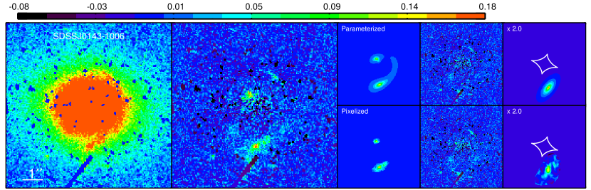
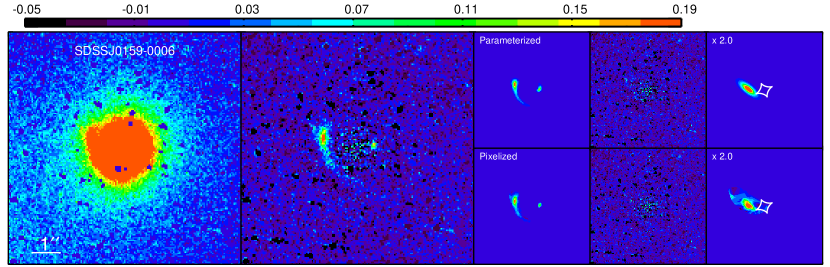
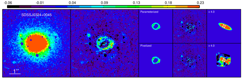
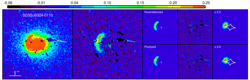
Figure 2.— SIE lens models for the 40 S4TM grade-A lenses. The observational data, B-spline-subtracted image, predicted lensed image, final residual, and the background source model are shown from left to right, respectively. Images are orientated such that north is up and East is to the left. For each system, the results of the two source models are split into two rows with the parameterized source model on the top and the pixelized source model on the bottom. The white lines in the last panels are the caustics of the lens model. The source plane panels are magnified by factors from 2 to 32 relative to the image plane panel as indicated in each panel. The color bars indicate the intensity levels in units of electrons per second per pixel². [The remaining 36 figures are available in the online journal.]

5. Discussion

The S4TM survey is optimized to select strong-lens systems with relatively lower-mass lens galaxies as a complementary sample to the SLACS sample. In Figure 3, we compare the stellar velocity dispersion, Einstein radius, total projected mass within the Einstein radius, and stellar mass between the two lens samples. The SLACS sample refers to the 63 grade-A lenses with lens models in Bolton et al. (2008a).

The distribution of the stellar velocity dispersions $\sigma_{\rm SDSS}$ of the S4TM sample has a strong peak at about 200 km s^-1 and declines rapidly on both ends. On the other hand, the distribution of $\sigma_{\rm SDSS}$ of the SLACS sample is almost flat from 200 to 320 km s^-1. As a comparison, the median $\sigma_{\rm SDSS}$ of the S4TM sample is 203 km s^-1 while it is 243 km s^-1 for the SLACS sample. The median Einstein radius of the S4TM sample is 1$\farcs$00, almost $15\%$ smaller than that of the SLACS sample (1$\farcs$17). The distributions of the Einstein radii for the two samples further suggest that the S4TM sample is more abundant in systems with Einstein radii smaller than 0$\farcs$8 (12/40 versus 3/63) and lack systems with Einstein radii larger than 1$\farcs$2 (8/40 versus 30/63). We basically expect the distributions of $M_{\rm Ein}$ to be similar to those of $b_{\rm SIE}$ because $\Sigma_{\rm crit}$, which is determined by the lens and source redshifts, distributes roughly the same for the two samples. The histogram in Figure 3 confirms this. The total projected mass within the Einstein radius $M_{\rm Ein}$ of the S4TM sample ranges from $3\times 10^{10}$ to $2\times 10^{11}M_{\odot}$. And the median $\log_{10}(M_{\rm Ein}/M_{\odot})$ of the S4TM sample is 11.02, 0.23 dex (almost a factor of 2) smaller than that of the SLACS lens galaxies. The stellar mass for these lens galaxies ranges from $3\times 10^{10}$ to $1\times 10^{12}M_{\odot}$. The S4TM grade-A lens galaxies are again less massive in stellar mass than SLACS grade-A lens galaxies. The difference in the median values is 0.26 dex. We also look at the ratio of the Einstein radius to the half-light radius for these two lens samples. The distributions appear almost the same and peak around 0.5. The median $b_{\rm SIE}/r_{\rm half}$ ratio of the S4TM sample is slightly larger than that of the SLACS sample (0.54 versus 0.48).

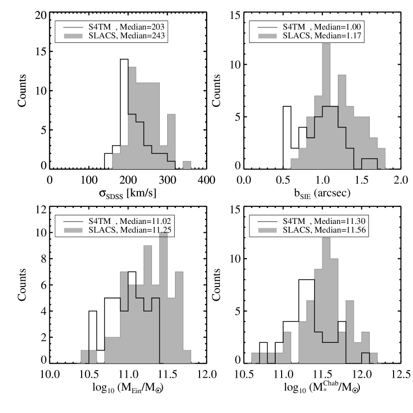
Figure 3.— Distributions of the stellar velocity dispersion, Einstein radius, total enclosed mass within the Einstein radius, and stellar mass for the S4TM (solid histograms) and the SLACS (dashed histograms) lens samples. The stellar mass is derived from HST F814W-band photometry assuming a Chabrier IMF as explained in Shu et al. (2015).

The comparatively less massive S4TM lens sample serves as a complementary addition to the current galaxy-scale strong-lens samples, which are usually biased toward more massive lens galaxies (e.g., Auger et al., 2010; Faure et al., 2011; Brownstein et al., 2012; Sonnenfeld et al., 2013). It extends the lens-galaxy mass coverage to the lower-mass end, and can allow a more thorough investigation of the mass structure and scaling relations of ETGs when combined with other strong-lens samples, especially the SLACS sample which is selected from the same parent sample with the same selection technique. For instance, we studied the mass structure of ETGs by combining S4TM and SLACS grade-A and grade-C lenses. Previous studies with only high-mass coverages showed that the total mass–density distribution of ETGs in strong-lens systems can be well approximated by an isothermal profile with little correlation with galaxy mass (e.g., Koopmans et al., 2006; Bolton et al., 2008b; Koopmans et al., 2009; Barnabè et al., 2011; Ruff et al., 2011). However, by including the relatively lower-mass S4TM grade-A lenses and also grade-C lenses, we found the total mass–density profile of ETGs varies systematically with galaxy mass with a 6$\sigma$ significance (Shu et al., 2015).

Although the S4TM sample does not reach as low as the lower characteristic mass scale of $3\times 10^{10}M_{\odot}$ in stellar mass, the broader mass coverage can still enable us to directly test, with the aid of strong lensing, for a transition in structural and dark-matter content trends at intermediate galaxy mass as noticed in previous studies (e.g., Tremblay & Merritt, 1996; Graham & Guzmán, 2003; van der Wel et al., 2009; Bernardi et al., 2011a, b; Cappellari et al., 2013a, b). Furthermore, the S4TM strong-lens sample can be a useful resource for testing general relativity (GR) by comparing dynamical mass and lensing mass (e.g., Bolton et al., 2006b; Jain & Zhang, 2008; Schwab et al., 2010; Cao et al., 2017). In particular, the extended mass coverage of the S4TM sample will provide extra constraints on GR by revealing the environmental dependence of dark-matter halo properties as demonstrated by the numerical simulations (e.g., Zhao et al., 2011; Winther et al., 2012; He et al., 2014). Lastly, we note that by further going to candidates with lower predicted lensing cross sections, we might be able to obtain a sample of strong-lens systems with even lower lens masses.

6. Summary

In this paper, we presented a catalog of 40 new galaxy-scale strong lenses confirmed by HST F814W-band imaging observations of 118 candidates in the S4TM survey, an extension of the SLACS survey toward lower lens-galaxy mass. The HST observational data are well explained by an elliptical B-spline model for the lens-light distribution, an SIE profile for the lens-mass distribution, and multiple Sérsic components for the source-light distribution. Our main findings are as follows.

1. The lens galaxies are ETGs at redshifts of $\sim 0.17$, and background sources are star-forming galaxies located at redshifts of $\sim 0.61$ with strong nebular emission lines (Balmer series, [Oii] 3727, or [Oiii] 5007).

2. The Einstein radius distribution of the S4TM lenses ranges from 0$\farcs$54 to 1$\farcs$62 with a median value of 1$\farcs$00. The fraction of systems with small Einstein radii ($<$ 0$\farcs$80) in the S4TM sample is a factor of 5 larger than that in the SLACS sample.

3. On average, the S4TM lenses are indeed less massive than those of the SLACS lenses. Based on our best-fit lens models, the total projected mass within the Einstein radius of the S4TM sample ranges from $3\times 10^{10}$ to $2\times 10^{11}M_{\odot}$ with a median mass of $1\times 10^{11}M_{\odot}$, which is smaller by almost a factor of 2 when compared to the SLACS sample. The SPS-derived stellar mass based on HST photometry also suggests that S4TM lenses are generally less massive than SLACS lenses by almost a factor of 2.

4. The extended mass coverage toward the low-mass end provided by the S4TM sample makes it a complementary addition to the current galaxy-scale strong-lens samples, and will also extend our understanding of ETGs. Shu et al. (2015), by including the relatively less massive S4TM grade-A lenses and grade-C lenses, detected a strong correlation between ETG mass and its total mass–density profile, which was not noticed in previous studies using only massive ETGs (e.g., Bolton et al., 2008b; Koopmans et al., 2009; Barnabè et al., 2011; Ruff et al., 2011). In addition, it enables us to probe intermediate-mass ETGs where transitions in scaling relations, kinematic properties, mass structure, and dark-matter content trends are detected (e.g., Tremblay & Merritt, 1996; Graham & Guzmán, 2003; Kauffmann et al., 2003; Graham & Worley, 2008; Hyde & Bernardi, 2009; Skelton et al., 2009; Tortora et al., 2009; van der Wel et al., 2009; Bernardi et al., 2011a, b; Cappellari et al., 2013a, b; Montero-Dorta et al., 2016).

References

- Abazajian et al. (2009) Abazajian, K. N., Adelman-McCarthy, J. K., Agüeros, M. A., et al. 2009, ApJS, 182, 543
- Auger et al. (2009) Auger, M. W., Treu, T., Bolton, A. S., et al. 2009, ApJ, 705, 1099
- Auger et al. (2010) —. 2010, ApJ, 724, 511
- Baldry et al. (2012) Baldry, I. K., Driver, S. P., Loveday, J., et al. 2012, MNRAS, 421, 621
- Barnabè et al. (2011) Barnabè, M., Czoske, O., Koopmans, L. V. E., Treu, T., & Bolton, A. S. 2011, MNRAS, 415, 2215
- Bernardi et al. (2011a) Bernardi, M., Roche, N., Shankar, F., & Sheth, R. K. 2011a, MNRAS, 412, 684
- Bernardi et al. (2011b) —. 2011b, MNRAS, 412, L6
- Bolton et al. (2008a) Bolton, A. S., Burles, S., Koopmans, L. V. E., et al. 2008a, ApJ, 682, 964
- Bolton et al. (2006a) Bolton, A. S., Burles, S., Koopmans, L. V. E., Treu, T., & Moustakas, L. A. 2006a, ApJ, 638, 703
- Bolton et al. (2004) Bolton, A. S., Burles, S., Schlegel, D. J., Eisenstein, D. J., & Brinkmann, J. 2004, AJ, 127, 1860
- Bolton et al. (2006b) Bolton, A. S., Rappaport, S., & Burles, S. 2006b, Phys. Rev. D, 74, 061501
- Bolton et al. (2008b) Bolton, A. S., Treu, T., Koopmans, L. V. E., et al. 2008b, ApJ, 684, 248
- Brewer & Lewis (2006) Brewer, B. J., & Lewis, G. F. 2006, ApJ, 637, 608
- Brewer et al. (2012) Brewer, B. J., Dutton, A. A., Treu, T., et al. 2012, MNRAS, 422, 3574
- Browne et al. (2003) Browne, I. W. A., Wilkinson, P. N., Jackson, N. J. F., et al. 2003, MNRAS, 341, 13
- Brownstein et al. (2012) Brownstein, J. R., Bolton, A. S., Schlegel, D. J., et al. 2012, ApJ, 744, 41
- Cao et al. (2017) Cao, S., Li, X., Biesiada, M., et al. 2017, ApJ, 835, 92
- Cappellari et al. (2013a) Cappellari, M., Scott, N., Alatalo, K., et al. 2013a, MNRAS, 432, 1709
- Cappellari et al. (2013b) Cappellari, M., McDermid, R. M., Alatalo, K., et al. 2013b, MNRAS, 432, 1862
- Chabrier (2003) Chabrier, G. 2003, PASP, 115, 763
- Cole et al. (2000) Cole, S., Lacey, C. G., Baugh, C. M., & Frenk, C. S. 2000, MNRAS, 319, 168
- Davidzon et al. (2017) Davidzon, I., Ilbert, O., Laigle, C., et al. 2017, ArXiv e-prints, arXiv:1701.02734
- de Vaucouleurs (1948) de Vaucouleurs, G. 1948, Annales d’Astrophysique, 11, 247
- Djorgovski & Davis (1987) Djorgovski, S., & Davis, M. 1987, ApJ, 313, 59
- Dressler et al. (1987) Dressler, A., Lynden-Bell, D., Burstein, D., et al. 1987, ApJ, 313, 42
- Dye & Warren (2005) Dye, S., & Warren, S. J. 2005, ApJ, 623, 31
- Ebeling et al. (2007) Ebeling, H., Barrett, E., Donovan, D., et al. 2007, ApJ, 661, L33
- Einstein (1916) Einstein, A. 1916, Annalen der Physik, 354, 769
- Faber & Jackson (1976) Faber, S. M., & Jackson, R. E. 1976, ApJ, 204, 668
- Faure et al. (2008) Faure, C., Kneib, J.-P., Covone, G., et al. 2008, ApJS, 176, 19
- Faure et al. (2011) Faure, C., Anguita, T., Alloin, D., et al. 2011, A&A, 529, A72
- Graham & Guzmán (2003) Graham, A. W., & Guzmán, R. 2003, AJ, 125, 2936
- Graham & Worley (2008) Graham, A. W., & Worley, C. C. 2008, MNRAS, 388, 1708
- He et al. (2014) He, J.-h., Li, B., Hawken, A. J., & Granett, B. R. 2014, Phys. Rev. D, 90, 103505
- Hyde & Bernardi (2009) Hyde, J. B., & Bernardi, M. 2009, MNRAS, 394, 1978
- Ilbert et al. (2010) Ilbert, O., Salvato, M., Le Floc’h, E., et al. 2010, ApJ, 709, 644
- Inada et al. (2012) Inada, N., Oguri, M., Shin, M.-S., et al. 2012, AJ, 143, 119
- Jain & Zhang (2008) Jain, B., & Zhang, P. 2008, Phys. Rev. D, 78, 063503
- Kauffmann et al. (1993) Kauffmann, G., White, S. D. M., & Guiderdoni, B. 1993, MNRAS, 264, 201
- Kauffmann et al. (2003) Kauffmann, G., Heckman, T. M., White, S. D. M., et al. 2003, MNRAS, 341, 33
- Kochanek et al. (2000) Kochanek, C. S., Falco, E. E., Impey, C. D., et al. 2000, ApJ, 543, 131
- Komatsu et al. (2011) Komatsu, E., Smith, K. M., Dunkley, J., et al. 2011, ApJS, 192, 18
- Koopmans (2005) Koopmans, L. V. E. 2005, MNRAS, 363, 1136
- Koopmans et al. (2006) Koopmans, L. V. E., Treu, T., Bolton, A. S., Burles, S., & Moustakas, L. A. 2006, ApJ, 649, 599
- Koopmans et al. (2009) Koopmans, L. V. E., Bolton, A., Treu, T., et al. 2009, ApJ, 703, L51
- Kormann et al. (1994) Kormann, R., Schneider, P., & Bartelmann, M. 1994, A&A, 284, 285
- Kormendy (1977) Kormendy, J. 1977, ApJ, 218, 333
- Li & White (2009) Li, C., & White, S. D. M. 2009, MNRAS, 398, 2177
- Maraston et al. (2013) Maraston, C., Pforr, J., Henriques, B. M., et al. 2013, MNRAS, 435, 2764
- Marques-Chaves et al. (2017) Marques-Chaves, R., Pérez-Fournon, I., Shu, Y., et al. 2017, ApJ, 834, L18
- Marshall et al. (2007) Marshall, P. J., Treu, T., Melbourne, J., et al. 2007, ApJ, 671, 1196
- Montero-Dorta et al. (2016) Montero-Dorta, A. D., Shu, Y., Bolton, A. S., Brownstein, J. R., & Weiner, B. J. 2016, MNRAS, 456, 3265
- More et al. (2012) More, A., Cabanac, R., More, S., et al. 2012, ApJ, 749, 38
- More et al. (2016) More, A., Verma, A., Marshall, P. J., et al. 2016, MNRAS, 455, 1191
- Muñoz et al. (1998) Muñoz, J. A., Falco, E. E., Kochanek, C. S., et al. 1998, Ap&SS, 263, 51
- Negrello et al. (2017) Negrello, M., Amber, S., Amvrosiadis, A., et al. 2017, MNRAS, 465, 3558
- Newville et al. (2014) Newville, M., Stensitzki, T., Allen, D. B., & Ingargiola, A. 2014, LMFIT: Non-Linear Least-Square Minimization and Curve-Fitting for Python¶, doi:10.5281/zenodo.11813
- Nightingale & Dye (2015) Nightingale, J. W., & Dye, S. 2015, MNRAS, 452, 2940
- Pawase et al. (2014) Pawase, R. S., Courbin, F., Faure, C., Kokotanekova, R., & Meylan, G. 2014, MNRAS, 439, 3392
- Ruff et al. (2011) Ruff, A. J., Gavazzi, R., Marshall, P. J., et al. 2011, ApJ, 727, 96
- Schlegel et al. (1998) Schlegel, D. J., Finkbeiner, D. P., & Davis, M. 1998, ApJ, 500, 525
- Schwab et al. (2010) Schwab, J., Bolton, A. S., & Rappaport, S. A. 2010, ApJ, 708, 750
- Shu et al. (2016a) Shu, Y., Bolton, A. S., Moustakas, L. A., et al. 2016a, ApJ, 820, 43
- Shu et al. (2015) Shu, Y., Bolton, A. S., Brownstein, J. R., et al. 2015, ApJ, 803, 71
- Shu et al. (2016b) Shu, Y., Bolton, A. S., Mao, S., et al. 2016b, ApJ, 833, 264
- Skelton et al. (2009) Skelton, R. E., Bell, E. F., & Somerville, R. S. 2009, ApJ, 699, L9
- Sonnenfeld et al. (2013) Sonnenfeld, A., Gavazzi, R., Suyu, S. H., Treu, T., & Marshall, P. J. 2013, ApJ, 777, 97
- Sonnenfeld et al. (2017) Sonnenfeld, A., Chan, J. H. H., Shu, Y., et al. 2017, ArXiv e-prints, arXiv:1704.01585
- Stark et al. (2013) Stark, D. P., Auger, M., Belokurov, V., et al. 2013, MNRAS, 436, 1040
- Suyu et al. (2006) Suyu, S. H., Marshall, P. J., Hobson, M. P., & Blandford, R. D. 2006, MNRAS, 371, 983
- Toomre & Toomre (1972) Toomre, A., & Toomre, J. 1972, ApJ, 178, 623
- Tortora et al. (2009) Tortora, C., Napolitano, N. R., Romanowsky, A. J., Capaccioli, M., & Covone, G. 2009, MNRAS, 396, 1132
- Tremblay & Merritt (1996) Tremblay, B., & Merritt, D. 1996, AJ, 111, 2243
- Treu (2010) Treu, T. 2010, ARA&A, 48, 87
- Treu et al. (2011) Treu, T., Dutton, A. A., Auger, M. W., et al. 2011, MNRAS, 417, 1601
- van der Wel et al. (2009) van der Wel, A., Rix, H.-W., Holden, B. P., Bell, E. F., & Robaina, A. R. 2009, ApJ, 706, L120
- Vegetti & Koopmans (2009) Vegetti, S., & Koopmans, L. V. E. 2009, MNRAS, 392, 945
- Vieira et al. (2013) Vieira, J. D., Marrone, D. P., Chapman, S. C., et al. 2013, Nature, 495, 344
- Walsh et al. (1979) Walsh, D., Carswell, R. F., & Weymann, R. J. 1979, Nature, 279, 381
- White & Frenk (1991) White, S. D. M., & Frenk, C. S. 1991, ApJ, 379, 52
- Winther et al. (2012) Winther, H. A., Mota, D. F., & Li, B. 2012, ApJ, 756, 166
- Yang et al. (2009) Yang, X., Mo, H. J., & van den Bosch, F. C. 2009, ApJ, 695, 900
- Zhao et al. (2011) Zhao, G.-B., Li, B., & Koyama, K. 2011, Physical Review Letters, 107, 071303