Nuclear Magnetic Resonance in High Magnetic Field: Application to Condensed Matter Physics

Abstract

In this review, we describe the potentialities offered by the nuclear magnetic resonance (NMR) technique to explore at a microscopic level new quantum states of condensed matter induced by high magnetic fields. We focus on experiments realised in resistive (up to 34 T) or hybrid (up to 45 T) magnets, which open a large access to these quantum phase transitions. After an introduction on NMR observable, we consider several topics: quantum spin systems (spin-Peierls transition, spin ladders, spin nematic phases, magnetisation plateaus and Bose-Einstein condensation of triplet excitations), the field-induced charge density wave (CDW) in high $T_{c}$ superconductors, and exotic superconductivity including the Fulde-Ferrel-Larkin-Ovchinnikov superconducting state and the field-induced superconductivity due to the Jaccarino-Peter mechanism.

I Introduction

Since its discovery just after the second World War, the nuclear magnetic resonance (NMR) technique has known a tremendous development in chemistry, biology and imaging for medical applications (MRI). This development was founded on three pillars: the development of superconducting magnets providing extremely stable and homogeneous ($10^{-10}$) magnetic fields up to 23.4 T (1 GHz for proton resonance), the continuously increasing power of computers, and the development of high frequency and high power electronics. Most of the experiments performed in the world concern structural information and are usually performed around room temperature (in particular for biology and MRI) in diamagnetic systems. The situation is quite different for NMR applied to solid state physics, where temperature, pressure and magnetic field are essential thermodynamic variables. The homogeneity and stability requirements are much less stringent than mentioned above, and usually fall in the range $10^{-5}-10^{-3}$, depending on the systems under study, so that in many cases all-purpose high-field resistive magnets, available only in few dedicated facilities in the world, can be used up to field values up to 35 T, or even 45 T in a hybrid magnet. In this case, high magnetic fields are not used to increase the sensitivity or the resolution of NMR spectroscopy, but as a physical variable able to induce phase transitions, even at zero temperature (the so-called quantum phase transitions) and to access to new (quantum) phases of condensed matter [Cargese, ]. Electrons in the matter couple to the magnetic field $H$ through their spin and orbit. In this latter case, it is convenient to define a typical magnetic length $l_{B}=\sqrt{\hbar/eB}=\frac{25\textrm{nm}}{\sqrt{B}[\textrm{T}]}$, such as $2\pi l_{B}^{2}B=\phi_{0}=h/e$, where $e$ is the absolute value of the electron charge, and $\phi_{0}$ the elementary flux quantum, and to compare it to some typical distance of the system under study. The most well known examples are the critical field $H_{c2}$ in a superconductor of type II and the Integer Quantum Hall Effect (IQHE) and the Fractional one (FQHE) in 2D electron gas. In the first case, the comparison between the coherence length $\xi$ of the Cooper pairs and the (superconducting) quantum flux $\phi_{0s}=h/(2e)$ gives the upper critical field $H_{c2}=\phi_{0}/2\pi(\xi(T))^{2}$ [De Gennes, ]. In the second case, the IQHE plateaus correspond to incompressible phases in which the number of electrons per flux quanta is an integer [Kitzing, ]. A similar picture can be used for the FQHE [Stormer, ] with composite fermions [Jain, ; GlattliShankar, ]. As far as the coupling with the spins are concerned, it is the Zeeman energy which has to be compared with relevant energy scale in the system under consideration. Examples range from quantum spin systems, in which the characteristic energies derive from the exchange couplings $J$’s, to the Pauli limit in superconductors when the Zeeman energy overcomes the pairing energy of Cooper pairs. More generally, application of magnetic field allows to generate new quantum phases and, until recently, NMR has been the only technique allowing a microscopic investigation of their structure and excitations for field values above 17 T. This is now changing, with the new possibilities for X-rays to do experiments under pulsed magnetic fields up to 30 T [Xraypulsedfields, ] and for neutron scattering up to 27 T [Berlin, ]. Comparing results obtained by these techniques with those obtained by NMR opens a new fascinating area of research.

In this paper, we will review some of the NMR contributions to the physics in high magnetic fields performed by the authors [FagotPRL, ; FagotPRB, ; ChaboussantPRL, ; Chaboussant_1998, ; HorvaticPRLCuGeO_99, ; Julien2000, ; Mladen_Cargese, ; Kodama2002, ; Takigawa2004, ; Kraemer2007, ; Hiraki_2007, ; Klanjsek_2008, ; Levy2008, ; Koutroulakis10, ; Tao2011, ; Mukhopadhyay_2012, ; Wu13, ; Tao2013, ; Takigawa2013, ; Kraemer2013, ; Jeong, ; Mayaffre14, ; Klanjsek_2015, ; Tao2015, ; Julien15, ; Iye, ; Jeong2016, ; Blinder2017, ; Orlova_2017, ; Zhou17, ; Zhou17b, ] using resistive magnets at the ”Laboratoire National des Champs Magnétiques Intenses” (LNCMI-Grenoble). Some experiments requiring magnetic fields up to 45 T were performed at the National High Magnetic Field Laboratory (NHMFL) at Tallahasse (Florida, USA) and we also discuss recent NMR results obtained in pulsed magnetic field up to 55 T at the LNCMI-Toulouse.

II NMR observables

Without entering into details of how NMR is actually performed [Slichter, ; Abragam, ; Mehring, ; Nuts, ; NarathNMR, ], we will limit the presentation to its basic principles in order to explain what physical quantities can be observed [Mladen_Cargese, ]. In a typical configuration, NMR relies on the Zeeman interaction

$$\mathcal{H}_{\mathrm{Z}}=-\bm{\mu}_{\mathrm{n}}\cdot\mathbf{H}_{\mathrm{n}}$$ (1)

of the magnetic moment of nuclei (of selected atomic species) $\mathbf{\mu}_{\mathrm{n}}=\hbar\gamma_{\mathrm{n}}\mathbf{I}_{\mathrm{n}}$, where $\gamma_{\mathrm{n}}$ and $\mathbf{I}_{\mathrm{n}}$ are the gyromagnetic ratio and the spin of the nucleus, to obtain an information on the local magnetic field value $\mathbf{H}_{\mathrm{n}}$ at this position. The experiment is performed in a magnetic field $H_{0}\sim 10$ T whose value is precisely known (calibrated by NMR), and which is perfectly constant in time and homogeneous over the sample volume. A resonance signal is observed at the Larmor frequency corresponding to transitions between adjacent Zeeman energy levels $\omega_{\mathrm{NMR}}=\gamma_{\mathrm{n}}H_{\mathrm{n}}$, allowing very precise determination of $\mathbf{H}_{\mathrm{n}}$, and therefore of the local, induced, so-called “hyperfine field” $\mathbf{H}_{\mathrm{hf}}=\mathbf{H}_{\mathrm{n}}-\mathbf{H}_{0}$ (as $\gamma_{\mathrm{n}}$ is known from calibration on a convenient reference sample). This hyperfine field, produced by the electrons surrounding the chosen nuclear site, is a signature of local electronic environment. On the other hand, nuclei which have a spin I $>$ 1/2 have a non-spherical distribution of charge, and possess a quadrupolar moment which couples to the electric field gradient (EFG) tensor produced by the surrounding electronic and ionic charges. In a single crystal, the single NMR line corresponding to the Zeeman interaction is then split into 2I lines, and this allows an accurate determination of the EFG tensor, a quantity very sensitive to structural transitions, or to a modulation of the electronic density, as observed in CDW systems [Berthier78, ]. While the NMR spectra correspond to static values (at the NMR scale) of the hyperfine field and the EFG, the fluctuations of these quantities are at the origin of the spin-lattice relaxation rate ($1/T_{1}$), which measures their spectral density at the Larmor frequency.

II.1 High Magnetic Field and NMR

The spectral resolution of NMR is directly limited by the temporal and spatial homogeneity of the external magnetic field $H_{0}$. In the experiments where NMR is used for the determination of complex molecular structures [HighRes, ], the $H_{0}$ field variations over the nominal sample dimension of 1 cm should be $\sim$ 10^-9 for studies in liquid solutions or 10^-6–10^-8 in solid state compounds. In both cases the magnetic field is produced by commercially available, “high-resolution” superconducting (SC) magnets, providing fixed field, limited by the present SC technology to a maximum field of 23.4 T. An SC magnet operating at 28 T, using High $T_{\rm{c}}$ superconductor technology, should be commercialized soon. The interest in high fields for structural investigations is driven by the improvement of the resolution and the sensitivity.

When NMR is used as a probe of the electronic and magnetic properties in solid state physics, the required field homogeneity is typically much lower, 10^-3–10^-5, but the field should preferably be variable (sweepable). Up to 20 T such a field is available from commercial SC “solid state NMR magnets”, with homogeneity of 10^-5–10^-6. Higher fields (up to a maximum of 45 T) are available from big resistive or hybrid (SC+resistive) magnets, but their homogeneity is not optimised for NMR. Still, a typical value of 40$\times$10^-6 over a 1–2 mm sample positioned precisely in the field center is satisfactory for a great majority of solid state NMR studies. However, because of small sample size requirement and very high running cost, one uses these big magnets only for NMR studies of magnetic field dependent phenomena like field induced phase transitions.

II.2 Local static observables

The general Hamilonian for a species of spin $\mathbf{I}$, gyromagnetic ratio $\gamma_{i}$ and quadrupole moment Q in a solid placed in a an external magnetic field $H_{\mathrm{0}}$ can be written as

$$\mathcal{H}=\mathcal{H}_{Zemann}+\mathcal{H}_{hyperfine}+\mathcal{H}_{quadrupolar}+\mathcal{H}_{spin-spin},$$ (2)

in which $\mathcal{H}_{Zemann}=\sum_{i}-\gamma_{i}\hbar H_{\mathrm{0}}I_{z}$, $\mathcal{H}_{spin-spin}$ corresponds to the nuclear-nuclear spin interaction and $\mathcal{H}_{hyperfine}+\mathcal{H}_{quadrupolar}$ will be defined below. For simplicity, we shall only consider the most common case where $\mathcal{H}_{Zemann}$ $\gg$ $\mathcal{H}_{hyperfine},\mathcal{H}_{quadrupolar}$, and $\mathcal{H}_{spin-spin}$. In that case, one only retains the secular parts of the perturbative Hamiltonians, which commute with $\mathcal{H}_{Zemann}$.

In absence of unpaired electrons in the system, $\mathcal{H}_{hyperfine}$ resumes to the so-called chemical shift [Abragam, ], usually neglected in most of the metallic and magnetic systems, except in some of them like the organic conductors, as discussed in section V. In all other cases, the hyperfine Hamiltonian is dominated by the coupling with unpaired electrons, which for one electron $\mathbf{s}$ at a distance $\mathbf{r}$ writes as

$$\mathcal{H}_{hyperfine.}=2\mu_{\rm{B}}\gamma_{n}\hbar\mathbf{I}\cdot[\frac{\mathbf{l}}{r^{3}}-\frac{\mathbf{s}}{r^{3}}+3\frac{\mathbf{r}(\mathbf{s}\cdot\mathbf{r})}{r^{5}}+\frac{8\pi}{3}\mathbf{s}\delta(\mathbf{r})].$$ (3)

The orbital coupling $\mathbf{l}\cdot\mathbf{I}/r^{3}$ is usually neglected at the first order, since the orbital moment $\mathbf{l}$ is quenched by the crystal field, except when the spin-orbit coupling cannot be neglected. However, it contributes to the second order producing a paramagnetic orbital shift, which has the same origin as the Van-Vleck susceptibility whatever one deals with magnetic insulators [AbgBln, ] or metallic systems [Winter, ]. The other terms are responsible for the following contributions to the hyperfine shift: the anisotropic dipolar one due to electrons with $l\neq 0$, the isotropic contact one (due to ”$s$” electrons), and the core-polarisation (isotropic and most of the times negative) due to the polarisation of the inner closed $s$-shell by the open $p$ or $d$ shells [AbgBln, ; Winter, ].

In the absence of quadrupole coupling, the frequency of a line in an NMR spectrum gives a direct access to the local magnetic field at the position of the chosen nucleus. More precisely, we get an average of the local field on the time scale of the measuring process, $\sim$ 10–100 $\mu$s for solid state NMR. For systems with localised electronic spins in particular, it is easy to see that the induced field is linearly dependent on the spin polarisation of the nearest electronic spin(s) [NarathNMR, ]

$$\omega_{\mathrm{NMR}}/\gamma_{\mathrm{n}}=\left|\mathbf{H}_{0}+\left\langle\mathbf{H}_{\mathrm{hf}}\right\rangle\right|=\left|\mathbf{H}_{0}+{\sum}_{k}\,-A_{\mathrm{n},k}\left\langle\mathbf{S}_{k}\right\rangle+\mathbf{C}_{\mathrm{n}}\right|\;.$$ (4)

This linear dependence defines the hyperfine coupling constant (tensor) $A_{\mathrm{n},k}$ of nucleus “n” to electronic spin $\left\langle\mathbf{S}_{k}\right\rangle$ at position $k$, while $\mathbf{C}_{\mathrm{n}}$ accounts for quadratic (second order orbital or van Vleck) contributions which are not sensitive to the spin direction, as well as (generally much smaller) contribution of other (unpolarised) closed-shell electrons. Hyperfine coupling will be very different according to the distance between nuclear and electronic spins:

• On-site ($\mathrm{n}=k$) hyperfine coupling is strong, $A\sim 1$–100 T, and is approximately known for a given spin configuration (standard reference is [AbgBln, ]).

• When the coupling is ”transferred” or ‘”supertransferred” by an exchange process (i.e., due to overlap of wave functions) from the first or second neighbour site, its value is generally impossible to predict.

• For any distant spins ($\mathrm{n}\neq k$), there is also a direct magnetic dipole coupling, which is precisely known for given geometry ($\propto\left|\mathbf{r}_{\mathrm{n}}-\mathbf{r}_{k}\right|^{-3}$), and is generally smaller than the (super)transferred hyperfine coupling.

The interaction Hamiltonian corresponding to hyperfine coupling is $\mathcal{H}_{\mathrm{n},k}=\hbar\gamma_{\mathrm{n}}\mathbf{I}_{\mathrm{n}}\cdot A_{\mathrm{n},k}\cdot\mathbf{S}_{k}$ , and the experimentally measured “magnetic hyperfine shift” $K$ is defined as the frequency shift with respect to the reference:

$$K(T)\equiv\omega_{\mathrm{NMR}}/\left(\gamma_{\mathrm{n}}H_{0}\right)-1={\sum}_{k}\,A_{\mathrm{n},k\,}\left(g_{k}\mu_{\mathrm{B}}\right)^{-1}\chi_{k}(T)+K_{0},$$ (5)

where $g_{k}$ and $\chi_{k}$ are the $g$-tensor and the magnetic susceptibility (per site !) tensor of the $k$ spins, $\mu_{\mathrm{B}}$ the Bohr magneton and $K_{0}$ the shift corresponding to $\mathbf{C}_{\mathrm{n}}$ term in (4). $K$ is a tensor whose different components are obtained for different orientations of $\mathbf{H}_{0}$. Regarding the left-hand side of (5), we remark that NMR spectra can be equivalently obtained either in a fixed external field $H_{0}$ as a function of frequency, or at a fixed frequency $\omega_{\mathrm{NMR}}$ as a function of magnetic field. This latter configuration is more convenient for very wide spectra, except when the physical properties of the sample strongly vary with $H_{0}$. Equation (5), which is equivalent to $\mathcal{H}_{\mathrm{n},k}$ or (4), indicates how the $A$ tensor can be measured by NMR: when the temperature dependence of “bulk” magnetic susceptibility $\chi_{\mathrm{macro}}$ is dominated by the spatially homogeneous contribution of a single spin species, $A$ is calculated from the slope $\Delta K(T)/\Delta\chi_{\mathrm{macro}}(T)$ . If $\left\langle\mathbf{S}\right\rangle$ is taken to be a number, then $A$ is given in units of magnetic field; for historical reasons, the number that is usually declared is the “hyperfine field” = $A/g\mu_{\rm{B}}$ (in Gauss/$\mu_{\mathrm{B}}$).

One application of the determination of the hyperfine field is to obtain the true temperature and (or) the field dependence of the magnetisation of the spin system, which can not always been obtained from bulk measurements since they may be dominated by the contribution of impurities at low temperature [Mendels2000, ]. Another very important point is to determine whether the magnetization is uniform, or distributed over a commensurate or incommensurate structure, as we shall see later.

In the case of metals, the hyperfine interaction is responsible for the Knight shift, which can be written in the general case of a transition metal as [Winter, ]:

$$K=K_{s}+K_{d}+K_{orb}+K_{dipolar}+K_{chem},$$ (6)

where $K_{s}(K_{d}$) are proportional to the density of state at the Fermi level of $s$ or $s-p$ band ($d$-band) respectively, $K_{orb}$ depends on the filling of the $d$-band and is proportional to the Van-Vleck susceptibility, and the chemical shift $K_{chem}$ is usually negligible. $K_{dipolar}$ exists only in presence of $p$ or $d$ bands, and depends on the symmetry of the lattice [Winter, ]. In 3-dimensional (3D) systems and in absence of phase transition, $K_{s}$ and $K_{orb}$ are usually $T$-independent, while $K_{d}$ is $T$-dependent. There are many other situations where the Knight shift strongly varies with the temperature: quasi-1D organic conductors, itinerant antiferromagnets or ferromagnets, heavy fermions, which we do not discuss here. However it is worth to say a word on the case of superconductors. Below $T_{\rm{c}}$, a gap opens in the density of state, so that the Knight shift $K$ will vanish at low temperature (except for the orbital and the chemical contribution). The $T$-dependence of $K$($T$) depends of the symmetry of the order parameter. In the case of an $s$-wave singlet superconductor, $K$ decreases exponentially at sufficiently low temperature, the residual constant shift being due to the orbital and the chemical contribution. For clean $d$-wave superconductors, due to the presence of nodes in the gap, a linear behaviour is expected at low temperature, after removal of the above mentioned residual contributions. For triplet superconductors, the situation is more complex and depends on the precise symmetry of the order parameter [Mineev, ].

Let us now introduce the quadrupolar interaction. Its Hamiltonian is the part of the electrostatic interaction between the nuclei and the electrons, which describes the interaction of the electric field gradient (EFG) traceless tensor $V_{\alpha\alpha}$ with the quadrupole moment $Q$ of the nuclei . It can be written in the frame of the principal axes $X,Y,Z$ of the EFG tensor as

$$\mathcal{H}_{quadrupolar}=\frac{eV_{ZZ}Q}{4I(2I-1)}[3I_{Z}^{2}-I(I+1)+\frac{1}{2}\eta(I_{+}^{2}+I_{-}^{2})],$$ (7)

where the axes are chosen to satisfy $|V_{ZZ}|\geq|V_{YY}|\geq|V_{XX}|$, which constrains the asymmetry parameter $\eta$=$\frac{V_{YY}-V_{XX}}{V_{ZZ}}$ to $0\leq\eta\leq 1$. If the quadrupolar coupling can be treated as a perturbation, it is more convenient to express this Hamiltonian in the laboratory frame where the quantization is along the direction $z$ of the applied field. For simplicity, we assume that $\eta=0$, and limit ourselves to the first order in perturbation. We can rewrite the Hamiltonian as

$$\mathcal{H}=\frac{h\nu_{Q}}{6}[\frac{1}{2}(3\cos^{2}\theta-1)(3I_{z}^{2}-I(I+1)],$$ (8)

where $\nu_{Q}=3eQV_{ZZ}/h2I(2I-1)$, $\theta$ is the angle between the $Z$ direction and the applied magnetic field $H_{0}$ and $I\geq 1$. In a single crystal, the single line whose position is defined by the Zeeman coupling $\gamma\hbar H_{0}(1+K)I_{z}$ is split into $2I$ equidistant components, separated by $\nu_{Q}(3\cos^{2}\theta-1)/2$. In powder samples, these 2I lines are thus distributed over a frequency range spanning $(2I-1)\nu_{\rm{Q}}$. For half-integer spins, there is a central line (corresponding to the (-1/2, 1/2) transition), which is not affected to the first order, while for integer spins there is no central line left. Note that nuclei can have several isotopes of different natural abundance, with different gyromagnetic ratio and different quadrupole moment. For example, a single Cu site (spin 3/2) with a specific electronic spin polarisation and a specific charge environment, will give rise to six different lines, 3 for ⁶³Cu and 3 for ⁶⁵Cu (see section 3.3).

It is easy to see that a distribution of quadrupolar couplings, due to disorder or to the presence a CDW [Berthier78, ; Butaud, ] will change the shape of the satellites lines by an order of magnitude larger than that of the central line. The shape of the satellite lines will crucially depend on the symmetry of the CDW, the number of the wave-vectors defining the modulation ($1q,2q,3q$), and of its commensurate or incommensurate character.

One also notices that a spin-density wave (SDW) induces a modulation of $K$ which usually is easily distinguished from a CDW since it will affect in the same way the central line and the satellites. However, a charge modulation also implies a modulation of $K$ (which is important in the study of organic conductors undergoing a charge-ordering transition [Hiraki, ], where the nuclei under study are usually the ¹³C ( spin 1/2, $Q=0$)). This effect on the spectrum is usually smaller than the associated quadrupolar perturbation, but it may happen that they are of the same order of magnitude, like in underdoped YBa₂Cu₃O_6+x discussed in section 4. In that case, the two phenomena can still be disentangled, but in a more subtle way.

To conclude this section on static NMR observables, it is important to say that in the most general case, where the symmetry is lower that tetragonal or trigonal, the general form of the Hamiltonian is more complicated than mentioned here. It depends on $\theta$ and $\phi$ which define the orientation of the magnetic field with respect to the main axes of the quadrupolar tensor, and for strong quadrupolar couplings it may also be necessary to fit the spectra to the results of a fully diagonalised Hamiltonian to determine accurately $\nu_{q}$, $\eta$ and $K(\theta,\phi)$.

II.3 Dynamic observables

There are essentially two dynamic quantities used in NMR applied to solid state physics, which are the spin-lattice relaxation rate $1/T_{1}$, and the spin-spin relaxation rate $1/T_{2}$. In the absence of static magnetic field or EFG gradients inhomogeneities, $T_{2}$ is merely the correlation time of the transverse magnetization. Most of the time and in all the experiments described here, the time decay of the transverse magnetization is dominated by the inhomogeneities, and spectra, $1/T_{1}$ and $1/T_{2}$ are measured using the spin-echo technique [Slichter, ; Abragam, ; Mehring, ; Nuts, ; NarathNMR, ; Mladen_Cargese, ]. Since we do not use $1/T_{2}$ in the following, we shall not say more on this quantity (see [Mladen_Cargese, ] for further information). $1/T_{1}$ measures the characteristic time for the longitudinal nuclear magnetisation $M_{z}$ ($z$$\parallel$$H_{0}$) to return to its thermal equilibrium value after a perturbation, which is usually a destruction or an inversion of $M_{z}$. It essentially measures the weight of the spectral density at the Larmor frequency of the time fluctuations of the local hyperfine field or of the quadrupole couplings. In the following, we shall consider only the fluctuations of the hyperfine field. In localised spin systems, the part of the hyperfine field of interest for the relaxation can be written as: $\delta\mathbf{h}(t)=\mathbf{h}(t)-<\mathbf{h}(t)>$ where $<\mathbf{h}(t)>$ is the time-average value at the NMR time scale. For an applied field along the $z$ direction,

$$1/T_{1z}=\frac{1}{2}\gamma_{n}^{2}\int_{-\infty}^{\infty}d\textrm{t}~{}\rm{e}^{i\omega_{NMR}t}\langle\delta\mathbf{h}_{+}(t)\delta\mathbf{h}_{-}(0)\rangle$$ (9)

which can be explicitly expanded as :

$$T_{1z}^{-1}=\frac{1}{2}\gamma_{\mathrm{n}}^{2}\int_{-\infty}^{\infty}d\textrm{t}~{}\rm{e}^{i\omega_{NMR}t}[(A_{xz}^{2}+A_{yz}^{2})\,\langle S_{z}(t)S_{z}(0)\rangle+(A_{xx}^{2}+A_{yx}^{2})\langle S_{x}(t)S_{x}(0)\rangle+(A_{yy}^{2}+A_{xy}^{2})\langle S_{y}(t)S_{y}(0)\rangle]$$ (10)

Note that for a hyperfine coupling tensor $A$ that is non-diagonal (in the laboratory frame) both parallel and transverse (to external field $H_{0}$$\parallel$$z$) spin–spin correlation functions contribute to the relaxation, while only the latter contribution is active if $A$ is diagonal. In general, $A_{\alpha\neq\beta}\neq 0$ as soon as $H_{0}$ is not parallel to a principal axis of the $A$ tensor, which leads to a complicated angular dependence of $T_{1}$. This introduces the longitudinal correlation $\langle S_{z}(t)S_{z}(0)\rangle$ function in the calculation of 1/$T_{1}$, which usually involves different relaxation mechanisms than those associated to the transverse one [Mladen_Cargese, ; ChaboussantPRL, ].

To take into account the coupling to several electronic spins we replace $A\cdot\vec{S}$ by $\sum_{\vec{r}}A(\vec{r})\cdot\vec{S}(\vec{r})=\sum_{\vec{q}}\,A(\vec{q})\cdot\vec{S}(-\vec{q})$ to get (assuming inversion and translation symmetry):

$$T_{1z}^{-1}=\frac{1}{2}\gamma_{\mathrm{n}}^{2}\sum_{\textbf{q}}\sum_{\alpha=x,y,z}(A_{x\alpha}^{2}(\textbf{q})+A_{y\alpha}^{2}(\textbf{q}))\int_{-\infty}^{\infty}d\textrm{t}\rm{e}^{i\omega_{\mathrm{NMR}}t}\langle S_{\alpha}(\mathbf{q},t)S_{\alpha}(-\mathbf{q},0)\rangle$$ (11)

A more general expression, which can also be used in the case of itinerant electronic systems, is obtained using the fluctuation-dissipation theorem:

$$T_{1z}^{-1}=k_{\mathrm{B}}T\gamma_{\mathrm{n}}^{2}\sum_{\mathbf{q}}\sum_{\alpha=x,y,z}(A_{x\alpha}^{2}(\mathbf{q})+A_{y\alpha}^{2}(\mathbf{q}))\chi_{\alpha\alpha}^{\prime\prime}(\mathbf{q},\omega_{\mathrm{NMR}})/(\omega_{\mathrm{NMR}}g_{\alpha\alpha}^{2}\mu_{\mathrm{B}}^{2})$$ (12)

In the case of simple metals with a single conduction band, the relaxation rate is often expressed as proportional to the square of the density of states at the Fermi Level $N$($E_{F}$) [Slichter, ; Winter, ]. Since the Knight shift if also proportional to $N$($E_{F}$), this leads to the famous Korringa relationship:

$$K^{2}T_{1}T=\frac{\hbar}{4\pi k_{\rm{B}}}(\frac{\gamma_{e}}{\gamma_{n}})^{2}=S_{0},$$ (13)

where $\gamma_{e}$ ($\gamma_{n}$) are respectively the electron (nuclear) gyromagnetic ratios and $k_{\rm{B}}$ the Boltzman constant. The ratio $K^{2}T_{1}T$ is used as an indicator of the dominant fluctuations in the system, since $K$ is proportional to $\chi\rm{(}\emph{q}=0\rm{)}$, while $T_{1}T$ is proportional to $\omega_{n}/{\sum_{q}}\chi"\rm{(}\emph{q},\omega_{n}\rm{)}$. In absence of electron-electron interaction, $\chi"\rm{(}\emph{q},\omega_{n}\rm{)}$ is flat and $\mathfrak{S}=K^{2}T_{1}T/S_{0}=1$. In presence of ferromagnetic fluctuations, $\chi"\rm{(}\emph{q},\omega_{n}\rm{)}$ it is peaked at $q$ = 0, so that $\mathfrak{S}$ is smaller than 1, while in presence of antiferromagnetic (AF) fluctuations, it is larger than 1. The situation is more complicated in transition metals, since $s-p$ band and $d$-band have to be treated separately. Moreover, within the $d$-band, the relaxation due to the core-polarization, dipolar or anisotropic interactions, and the orbital relaxation have to be treated separately [NarathNMR, ; Winter, ]. $1/T_{1}$ is also very important to characterise superconductors. In $s$-wave superconductors, a gap opens on the whole Fermi surface, so that the relaxation rate decreases exponentially at low temperature. Just below $T_{\textrm{c}}$, due to a divergence of the density of states and the so-called coherence factor of the BCS theory, one should in principle observe the so-called Hebel-Slichter peak [HebelSlichter, ] in the relaxation rate. This peak is a hallmark of a singlet $s$-type superconductor, but its non-observation doesn’t mean that the order parameter is not $s$-like. This peak is absent in $p$ or $d$ type superconductors [Mineev, ]. For $d$-type singlet pairing, the gap vanishes at nodes, around which the density of states is linear as a function of the energy. As a consequence, the Knight shift varies linearly as a function of $T$, while $\rm{(}$$T_{1}T$$\rm{)}^{-1}$ is proportional to $T^{2}$. In cuprate high $T_{\rm{c}}$ superconductors, which are $d$-wave, this behavior is usually difficult to observe, due to impurities. In quasi-2D organic conductors, which are very pure, this behaviour can be observed when the field is parallel to the superconducting planes. In that case, there are no more Abrikosov vortices, so the contribution of their cores to the relaxation disappears. Only Josephson vortices are present, which do not contribute to $1/T_{1}$ [Mayaffre95, ] (see also section 5).

III Quantum spin systems under applied magnetic field

III.1 Introduction

Although a spin is by essence a quantum object, the denomination “quantum spin systems” (QSS) is usually dedicated to systems of localized electronic spins having small spin values (1/2, 1, … , for which the eigenvalues $S(S+1)$ of $\overrightarrow{S}^{2}$ strongly differ from $S^{2}$) and which are dominantly coupled by AF exchange interactions. In low-dimensional systems, thermal and quantum fluctuations are enhanced, and can destabilize the semi-classical long-range-order ground states of Néel type [Auerbach, ; Schollwock, ; Giamarchi_book, ; Sachdev_book, ; Frustration_book_2011, ]. Although the 1D spin chains have been studied very early by theorists, they are still an important playground to study experimentally modern concepts in magnetism, like, for example, quantum criticality, fractional excitations (spinons) and topological order. Moreover, since 1D spin systems can be mapped onto 1D strongly interacting spinless fermions through the Jordan-Wigner transformation [Jordan_Wigner, ], they allow, at the difference of other 1D systems like organic conductors, nanotubes or quantum wires, an accurate verification of the predictions of the Tomonaga-Luttinger liquid (TLL) model [Giamarchi_book, ], starting from the microscopic Hamiltonian [Klanjsek_2008, ]. Concerning quasi-2D spin systems, high $T_{\rm{c}}$ superconductors have promoted the search for exotic quantum ground states, notably after the suggestion by P.W. Anderson that they could be described as “a resonant valence bond (RVB) systems” doped by holes or electrons [Anderson, ]. The purpose of this paper is to show how important is the magnetic field in the physics of QSS, and to concentrate on their microscopic properties and low-energy excitations. Several techniques like neutron scattering [Broholm, ], EPR [Motokawa, ], and NMR [Mladen_Cargese, ] can give access to the microscopic properties of these new states, the most powerful being neutron scattering. This technique is however presently limited to magnetic fields lower than 17 T, even though inelastic neutron scattering experiments up to 27 T should become available soon [Berlin, ]. This section is limited to NMR in QSS under high magnetic fields, and to experiments on systems in which the magnetic field plays a key role, as a parameter of the phase diagram or the spin-dynamics. This will cover NMR experiments in quasi-1D spin chains and spin ladders [Schollwock, ; Giamarchi_book, ], magnetization plateaus [Takigawa_11, ] and Bose-Einstein condensation (BEC) in coupled dimer systems [Giamarchi_natphys, ; Zapf2014, ].

The general Hamiltonian of QSS can be written as $\mathcal{H}=\sum_{i,j}\overrightarrow{S}_{i}\mathbf{J}_{ij}\overrightarrow{S}_{j}+\mathcal{H}_{pert}$, where $\mathbf{J}_{ij}$, the exchange interaction (in most of the cases AF) between spins $\overrightarrow{S}_{i}$, is taken to be symmetric and can thus be written as $\mathbf{J}_{ij}=\sum_{\alpha}J_{ij}^{\alpha\alpha}$. The perturbation Hamiltonian $\mathcal{H}_{pert}$ can correspond to the Dzyaloshinskii-Moriya (DM) interaction [Dzyaloshinskii, ; Moriya, ] or staggered $g$-tensors, which both correspond to antisymmetric operators mixing the eingenstates of $S^{2}$, to the spin-phonon interaction, and (or) to the spin-spin dipolar interaction. In addition to the semi-classical ground states of Néel type, two categories of ground states have to be distinguished. The basic element of both of them is the so-called valence bond (VB) state, that is a pair of spin 1/2 forming a singlet state. The first family is formed by systems which can be separated in two distinct sublattices (bipartite systems). The ground state is usually a Valence Bond Crystals (VBC), in which there is no long range order (LRO) for the spins, but there is one for the valence bonds. Typical cases are spin ladders with strong rung couplings, and more generally weakly coupled spin dimer systems. The second one gathers the geometrically frustrated systems, the archetype of which being the 2D kagome lattice, which are expected in some case to have a spin liquid ground state [Frustration_book_2011, ; Balents, ]. In such a state, there is no longer any LRO, neither for the spins nor for the valence bonds, but the ground state is a quantum superposition of many valence bonds configurations. In this section we will mostly consider the systems in which the ground state in zero field is a collective singlet state, separated from the first excited triplet states by an energy gap $\Delta(0)$ (at $H=0$) which can be closed at a magnetic field $H_{\rm{c}}$ $=\Delta(0)/g\mu_{\textrm{B}}$. We shall distinguish quasi-1D systems, like spin chains and spin ladders, which by using the Jordan-Wigner transformation [Jordan_Wigner, ] can be mapped on interacting spinless fermions and, in most of the cases, described in the framework of Tomonaga-Luttinger liquid (TLL), and quasi-2D or 3D weakly coupled dimers in which the triplet excitations are rather described as hardcore bosons (or ”triplons”), for which the applied magnetic field plays the role of the bare chemical potential [Giamarchi_natphys, ]. These triplons can undergo a BEC [Giamarchi_natphys, ; GiamTsvelik1999, ; Nikuni2000, ] when their kinetic energy dominates their repulsion, while in the inverse situation, the triplons crystallise into magnetization plateaus for commensurate values of the triplets density [Takigawa_11, ; Rice2002, ].

III.2 Quasi-1D systems

In the absence of perturbation, the spin 1/2 chains can be described by the XXZ Hamiltonian

$\mathcal{H}=\sum_{i}J\{\epsilon(S_{i}^{x}S_{i+1}^{x}+S_{i}^{y}S_{i+1}^{y})+S_{i}^{z}S_{i+1}^{z}\}$. For $\epsilon\geq 1$, there is no gap in the low-energy excitations at all values of the magnetic field and the spin-spin correlation functions $\langle S_{+}(0,0)S_{-}(R,t)\rangle$ (transverse) and $\langle S_{z}(0,0)S_{z}(R,t)\rangle$ (longitudinal) decay as power laws with exponents $\eta_{x}$ and $\eta_{z}$. The transverse correlation function, which decays more slowly than the longitudinal one $\eta_{x}<\eta_{z}$, becomes dominant for low energy properties. If $\epsilon<1$, the ground state is of Néel type and separated from the excited states by a gap $\Delta(0)$, and can be closed at $H=H_{\textbf{c}}$. For $H\geq H_{\textbf{c}}$, the system enters into a TLL phase in which the longitudinal correlations are dominant at low energy [Haldane, ; Kimura_2008b, ]. However, increasing the magnetic field (i.e. the filling of the spinless fermions band), the exponents $\eta$ governing the decay of both correlation functions cross, and above a second critical field $H^{*}_{c}$, the transverse one becomes dominant.

Due to the inter-chain couplings that are always present in real compounds, these systems enter into a 3D ordered state at finite temperature. For $\epsilon\geq 1$, between $H=0$ and the saturation field $H_{s}$, this is a canted transverse AF state, while for $\epsilon<1$ this is a longitudinal, incommensurate, spin density wave between $H_{\rm{c}}$ and $H^{*}$, followed by a canted AF state between $H^{*}$ and the saturation field $H_{s}$. As an example, the spin system BaCo₂V₂O₈ has been the subject of intense investigation these last years [Kimura_2007, ; Kimura_2008, ; Canevet_2013, ; Grenier_2015, ; Klanjsek_2015, ].

In the presence of a perturbation, like an alternation of the exchange coupling, a frustrating nearest neighbour coupling, or a spin-phonon coupling, the spin-chains become gapped. As described above, the application of a magnetic field can close the gap and allows the system to enter into a TLL regime. As an example requiring the use of resistive magnet for NMR investigation, we describe below the case of the spin-Peierls compound CuGeO₃. We shall also mention the case of spin ladders, and that of the frustrated spin 1/2 chain LiCuVO₄ which is expected to present a nematic phase at high magnetic field around 45-50 T.

III.2.1 The High Field Phase of the spin-Peierls compound CuGeO₃

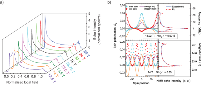
Figure 1: (Color online) (a) Evolution of the Cu NMR lineshape as a function of the applied magnetic field in CuGeO₃ above the critical field $H_{\textrm{c}}$. (b) left panels: Reconstruction of the real space spin-polarisation profile for $H$ = 13.02 and 24 T using Jacobi elliptic functions [HorvaticPRLCuGeO_99, ]. right panels: The corresponding fit (dashed line) superposed on experimental NMR lineshape ( full line), taken in the incommensurate high magnetic field phase of the spin–Peierls compound CuGeO₃. In this way, NMR lineshape has provided the precise magnetic field dependence of the average and staggered spin-polarisation and the magnetic correlation length up to 2$H_{\rm{c}}$ [HorvaticPRLCuGeO_99, ].

A spin–Peierls chain is a Heisenberg, AF, $S=1/2$ chain on an elastic lattice, in which the exchange interaction coupling depends on the position of the magnetic atoms, which can vary to minimize the total energy [Bray, ]. At low temperature, this spin chain can gain energy by spontaneous dimerisation (deformation) of the lattice, which allows the opening of a gap in the low-energy magnetic excitations (absent in simple Heisenberg half-integer spin chains). This dimerised phase has a non-magnetic collective singlet ground state and an energy gap towards triplet excitations. Application of magnetic field reduces the gap and, above the critical field $H_{\textrm{c}}$, drives the system into a magnetic phase with spatially inhomogeneous magnetisation (Fig. 1). In this field-induced phase, magnetisation appears as an incommensurate (IC) lattice of magnetisation peaks (solitons), where each soliton is bearing a total spin 1/2. The most studied spin–Peierls system is the inorganic compound CuGeO₃ [Hase, ], presenting a spin–Peierls transition at 14–10 K (depending on $H$), and a critical field $\simeq 13$ T. The NMR in CuGeO₃ has been performed on the “on-site” copper nuclei which are directly and very strongly coupled to the electronic spin. In the high-temperature and in the dimerised phase, symmetric NMR lines are observed, reflecting spatially uniform magnetisation. Comparing $K(T)$ vs. $\chi_{\mathrm{macro}}(T)$ the complete hyperfine coupling tensor as well as the orbital shift tensor $K_{0}=K(T=0)$ could be determined, and were found in good agreement with the values expected for a $d_{X^{2}-Y^{2}}$ orbital of Cu⁺⁺ ion [AbgBln, ; FagotPRB, ].

Above $H_{\rm{c}}$ each line is converted to a very wide asymmetric spectrum (Fig. 1) corresponding to a spatially non-uniform distribution of magnetisation. This NMR lineshape is in fact the density distribution of the local magnetisation, i.e., of the spin polarisation. Therefore, for a periodic function in 1D, it can be directly converted to the corresponding real-space spin-polarisation profile (soliton lattice, shown in Fig. 1 [FagotPRL, ; HorvaticPRLCuGeO_99, ]. It was thus possible to obtain a full quantitative description of the $H$ dependence of the spin-polarisation profile in the range from $H_{\rm{c}}$ to 2$H_{\rm{c}}$ = 26 T [HorvaticPRLCuGeO_99, ], clearly showing how the modulation of magnetisation evolves from the limit of nearly independent solitons just above $H_{\mathrm{c}}$, up to the high magnetic field limit, where it becomes nearly sinusoidal. Analysis of these data proved that the staggered component of magnetisation is reduced in the NMR image by phason-type motion of the soliton lattice [Uhrig, ; Ronnow, ]. The magnetic correlation length is found to be smaller than that associated to the lattice deformation (measured by X-rays [Kiryhukin, ]), which is a direct consequence of the frustration due to the second neighbour interaction in the system [Uhrig, ]. The observed field dependence of the correlation length remains to be understood.

III.2.2 Spin ladders

Spin ladders are 1D systems made of two (or more) coupled spin chains. First discussed as a by-product of high $T_{\rm{c}}$ cuprates [Hiroi, ; Dagotto, ], they present a rich phase diagram in the $H-T$ plane [Chaboussant_1998, ; Mila_98, ; Rice_Cargese, ], as shown on Fig. 2 . We shall consider here only the most simple type of $S~{}=~{}1/2$ two-legs ladders, described by the following Hamiltonian: $\mathcal{H}=\sum_{i}^{l=1,2}J_{\|}\overrightarrow{S}_{i}^{l}.\overrightarrow{S}_{i+1}^{l}+J_{\bot}\sum_{i}\overrightarrow{S}_{i}^{1}.\overrightarrow{S}_{i}^{2}$ where $J_{\|}$ ($J_{\bot}$) is the isotropic AF interaction along the legs (rungs). Whatever is the ratio $J_{\bot}/J_{\|}$, the ground state of two-legs spin ladders is the collective singlet separated by a gap from the first triplet excited states. As for the spin chains, the spin ladders can be described in terms of spinless fermions. But here the filling of the band starts from zero at the magnetic field $H_{\rm{c}}$ which closes the gap, up to the complete filling at $H_{\rm{s}}$. This is different from the case of the spin chains, where the filling starts always at half-filling at zero field. At temperature high enough to neglect the inter-ladder couplings, and low enough as compared to the Fermi energy of the spin-less fermions, the low-energy excitations can be described in the framework of a TLL.

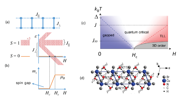
Figure 2: (Color online) (a) Schematic representation of a simple spin ladder . (b) Schematic representation of the energy levels as a function of the applied magnetic field $H$ in the case of a strong rung coupling. For a single dimer (rung), the first triplet excitation is separated from the singlet ground state by a gap $\Delta(H=0)=J_{\perp}$. Due to the interactions $J_{\parallel}$ along the legs, the triplet excitations form a band, which splits into three under the application of $H$. The lowest band first crosses the collective singlet ground state at the field $H_{\rm{c}}$ (closure of the gap). This corresponds to the first quantum critical point [Sachdev_book, ], at which the ground state switches from a gapped phase to a gapless one, which is described as a spinless, interacting, 1D fermion system (Tomonaga-Luttinger liquid) [Giamarchi_book, ]. The filling of the spinless fermion band increases as a function of $H$ up to the second critical field $H_{\textrm{s}}$ corresponding to the complete filling of the band. The point ($H=H_{\textrm{s}}$, $T=0$) is the second quantum critical point separating the gapless TLL from a gapped ($\Delta$ = $g\mu_{\textrm{B}}(H-H_{\textrm{s}})$) fully polarized phase. This scheme also applies to strong-leg coupling spin ladders, and $S=1$ spin chains (Haldane systems [Haldane_conjecture, ]), although their ground states and the gap are of different nature. The same energy scheme applies to all quasi-2D or 3D systems of weakly coupled spin dimers, but between $H_{\textrm{c}}$ and $H_{\textrm{s}}$ these systems are described as itinerant hard-core bosons on a lattice [Giamarchi_natphys, ], which ultimately condense at low temperature. (c): Phase diagram of a spin ladder in the $H-T$ plane. Above each of the two quantum critical points, there is a quantum critical regime in which the only energy scale is the temperature [Mukhopadhyay_2012, ]. For $E_{\rm{F}}\gg k_{\textrm{B}}T\gg J_{3D}$, where $E_{\rm{F}}$ is the Fermi energy of the spinless fermion band and $J_{3D}$ is the sum of the inter-ladder interactions, the system can be described as a TLL, while for $J_{3D}>k_{\textrm{B}}T$, a 3D LRO is established, which can be described as a Bose-Einstein condensation of magnons [GiamTsvelik1999, ]. (d): Structure of a strong rung coupling spin ladder (C₅H₁₂N)₂CuBr₄ (BPCB), from [Klanjsek_2008, ].

Finding systems which are true spin ladders, with values of the AF couplings comparable to the energy scale of the Zeeman coupling for fields accessible in the laboratory, is not so easy. An early candidate has been Cu₂(C₅H₁₂N₂)₂Cl₄ (called Cu(Hp)Cl) [Chaboussant_1998, ], presenting a phase diagram in the $H$-$T$ plane quite similar to that expected for a spin ladder , but the one-dimensionality of the system was questioned by neutron experiments [Stone_2000, ]. Recently, two spin ladder compounds, well characterised by NMR, neutron spectroscopy and thermodynamic measurements, have been the subject of intense experimental and theoretical studies. The first one, (C₅H₁₂N)₂CuBr₄, usually called BPCB but also known as (Hpip)₂CuBr₄) [Paytal, ; Watson, ], is a strong rung coupling spin ladder ($J_{\bot}\gg J_{\|}$) with a $H_{\rm{c}}$  = 6.7 T and $H_{\rm{s}}$ = 11.9 T [Klanjsek_2008, ]. The whole phase diagram in the H-T plane was studied by NMR [Klanjsek_2008, ], specific heat [Ruegg, ], and neutron spectroscopy [Thielemann, ], and the results compared to Density Matrix Renormalisation Group DMRG and bosonization calculation using the values of $J_{\bot}$ and $J_{\|}$ derived from experiments. The variation of the nuclear spin-lattice relaxation rate $1/T_{1}$ at fixed $T$ could be remarkably fitted in the whole interval $H_{\rm{c}}$ to $H_{\rm{s}}$  using a single parameter, the hyperfine coupling. Similarly, the field dependence of the transition temperature $T_{\rm{c}}$ of the 3D phase as well as that of its order parameter could be fitted using as a single parameter, the interchain coupling $J^{\prime}$. Using time-dependent DMRG, even the high energy excitations observed by inelastic neutron scattering could be very well reproduced, starting from the known values $J_{\bot}$ and $J_{\|}$ of the Hamiltonian [Bouillot, ].

The second spin ladder compound, (C₇H₁₀N)₂CuBr₂ (called DIMPY) [Shapiro, ], is in the strong-leg coupling regime ( $J_{\|}>J_{\bot}$) [Hong, ; Schmidiger, ] with $H_{\rm{c}}$  = 3 T and $H_{\rm{s}}$ = 29 T [Jeong2016, ]. This spin ladder belongs to the regime where the quasi particles are attractive ($K\geq 1$). Although the determination of the TLL parameter $K$ from $1/T_{1}$ is difficult [Jeong, ], the variation of $1/T_{1}$ as a function of $H$ between $H_{\rm{c}}$  = 3 T and $H_{\rm{s}}$ = 29 T measured at constant temperature $T$ = 750 mK [Jeong2016, ] was perfectly described by the Luttinger liquid parameters $K$($H$) and $u$($H$) determined from the starting Hamiltonian where $J_{\|}$ and $J_{\bot}$ have been determined from neutron spectroscopy.

In conclusion, spin ladders offer a rare example in which the TLL parameters can be computed directly from the microscopic parameters of the Hamiltonian. In that sense, they are perfect simulators of interacting spin-less fermions.

III.2.3 The nematic phase in frustrated $J_{1}-J_{2}$ chain. The LiCuVO₄ compound.

In spin systems, the frustration of the exchange couplings is known to lead to exotic ground states [Frustration_book_2011, ]. Here we describe the case of the spin nematic phase, for which the compound LiCuVO₄ seems to be the most promising system. LiCuVO₄ belongs to the class of the frustrated $J_{1}-J_{2}$ spin chains, in which the first neighbour exchange interaction $J_{1}$ is ferromagnetic (FM), while the next nearest neighbour is AF [Enderle, ]. In such a system, the saturated FM state at $H_{\rm{s}}$ was shown to be unstable with respect to the formation of pairs of bound magnons [Hikihara, ; Sudan, ; Zhitomirsky, ]. In their domain of stability, these bound magnons give rise to an SDW phase, in which the transverse fluctuations are gapped, and, just before the saturation to a nematic phase, in which the order parameter does not transform as a vector, but as a quadrupolar tensor of the type $S^{i}_{+}S^{i+1}_{+}+cc$. At lower field, single-magnon excitations prevail, giving rise to a vector chiral phase. The planar vector chiral phase and the longitudinal SDW attributed to the bound magnons have indeed been observed [Enderle, ; Buttgen_2012, ; Nawa, ] and here we focus only on the nematic phase. The search for this phase in LiCuVO₄ was triggered by the observation of an anomaly in the magnetisation curve just below the saturation field (45 T for $H\|c$, 52 T for $H\|b$) [Svistov, ]. At such a high field, the only available microscopic technique is the NMR. The first experiment was done for $H\|c$ in a steady magnetic field [Buttgen_2014, ], using the hybrid magnet at Tallahassee. It was concluded that the anomalous phase observed by magnetisation was essentially due to impurities, most of the system being saturated above 41.4 T, and that the nematic phase, if present, could only exist between 40.5 T $<H<$ 41.4 T. However, very recent experiments conducted in pulsed magnetic field for $H\|c$ and $H\|b$ have shown that, in both orientations, there is a field range below the saturation field in which there is no transverse order and the observed field dependence of the hyperfine shift is identical to the change in the magnetic susceptibility [Orlova_2017, ; Mila_2017, ], in agreement with the theoretical predictions for a nematic phase. Further evidence could be given by measuring $1/T_{1}$ as a function of temperature from the partially polarised phase down into the nematic one (at fixed value of $H$) [Smerald, ], but this type of measurement at such high magnetic fields are very challenging.

III.3 Magnetisation plateaus in the quasi-2D Shastry-Sutherland compound SrCu₂(BO₃)₂

The Shastry-Sutherland Hamiltonian (SSH) [Shastry, ] describes a 2D network of orthogonal dimers, which applies to SrCu₂(BO₃)₂ [Kageyama1999, ], the prototype compound for the study of magnetisation plateaus. In the SSH, one considers a square lattice that is paved by orthogonal dimers with an AF exchange $J$ along the diagonals (next nearest neighbours), and then introduce an frustrating AF coupling $J^{\prime}$ between each nearest neighbours. The product of singlets on the dimers is always an eigenstate of the SSH, whatever is the ratio $J^{\prime}/J$, but it remains the ground state only for $J^{\prime}/J<0.67$. For larger values of $J^{\prime}/J$, it enters a narrow plaquette phase [Koga2000, ; Corboz2013, ] before turning to a Néel ground state. In the SrCu₂(BO₃)₂ compound $J^{\prime}/J=0.63$, so the ground state is the product of singlets on each dimer. However, the hopping of a triplet from one dimer to its nearest neighbour is strongly restricted, favoring the existence of magnetisation plateaus. The first evidence for their existence in SrCu₂(BO₃)₂ was obtained by magnetisation measurements in pulsed magnetic field [Onizuka2000, ] with the observation of three plateaus at 1/8, 1/4 and 1/3 of the saturation magnetization. The first microscopic insight of the spin pattern of the 1/8 plateau was obtained soon after by Cu NMR in a resistive magnet at the LNCMI [Kodama2002, ; Takigawa2004, ], opening a long term collaboration between the Grenoble NMR group with that of M. Takigawa at the Institute of Solid State Physics at Tokyo.

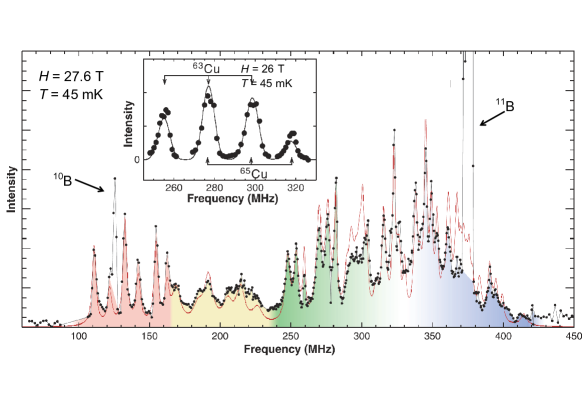
Figure 3: (Color online) Cu NMR spectrum in the 1/8 plateau of SrCu₂(BO₃)₂. The spectrum extends over $\simeq$ 300 MHz, corresponding to a range of $\simeq$ 30 T for the histogram of the hyperfine fields. To each site correspond 6 lines due to the two isotopes ⁶³Cu and ⁶⁵Cu and the quadrupole coupling, which does not depend on the site. Note that the width of stability of the plateau is only $\simeq$ 1.5 T which precludes any field sweep at constant frequency to obtain the full spectrum. From Ref. [Kodama2002, ].

As observed in the inset of Fig. 3, a single site of Cu (6 lines) is observed as long as the magnetisation grows from zero in the gapped state to the plateau, meaning a uniform polarisation of the Cu²⁺ electronic spins. The main figure shows that inside the plateau at least 10 different sites (60 lines) appear, spread over a distribution of internal field ${}^{63,65}A_{hyp}^{onsite}<S_{z}>$ of the order of 30 T. In particular, two strongly polarized sites are well resolved on the left of the spectra (the on-site hyperfine coupling for the Cu nuclei being strongly negative, Cu lines corresponding to strongly polarised Cu sites are strongly shifted to low frequency). Although the NMR spectra clearly demonstrate that the triplets crystalise within a commensurate super cell, they only give the histogram of the internal field due to these crystalised triplets but not the real magnetic structure inside the unit super cell, nor its symmetry. Exact diagonalisation of the Heisenberg SSH on a 16 spins cluster led to the conclusion that the unit cell (16 Cu²⁺ spins per layer) was rhombohedral, with oscillations of the spin polarization inside. Further calculations for the 1/4 and 1/3 plateaus showed the existence in all cases of strongly polarised “dressed triplet” extending on three dimers, forming stripes.

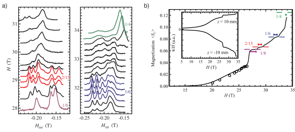
Figure 4: (Color online) Observation of the four plateaus at 1/8, 2/15, 1/6 and 1/4 in SrCu₂(BO₃)₂. (a) partial ¹¹B NMR spectra between 28 T and 34 T. Within the plateaus, the internal field histogram doesn’t change with the magnetic field, and the lines are sharp. (b) magnetization measurement (main figure) obtained from torque measurements (inset). One clearly observes the plateaus at 1/8, 2/15 and 1/6 of the magnetisation at saturation $m_{sat}$. From Ref. [Takigawa2013, ].

Further torque measurements [Levy2008, ; Sebastian2008, ] showed that the plateau sequence was not limited to 1/8, 1/4 and 1/3. While Ref. [Levy2008, ] reported the existence of a second plateau adjacent to the 1/8 also observed through ¹¹B NMR, Ref. [Sebastian2008, ] claimed the existence of a full series of plateaus at values of $\frac{m_{z}}{m_{sat}}=1/q$ (2 $\leq~{}q~{}\leq 9$ ) and 2/9. This was followed by new theoretical attempts to calculate the sequence of plateaus and their stability [Dorier2008, ; Abendschein2008, ], rendered difficult by the proximity of the quantum critical point at $J^{\prime}/J=0.67$, by the necessity to take into account long range interaction between the triplets as well as the additional terms to the SSH Hamiltonian like Dzyaloshiskii-Moriya interaction [Nemec2012, ]. With improvement of the pulse magnetic field set-ups, the 1/2 plateau was observed starting at 84 T [Jaime2012, ] and ending at 118 T [Matsuda2013, ]. The exact sequence of plateaus up to the 1/4 one, that is $\frac{m_{z}}{m_{sat}}=$ 1/8, 2/15, 1/6 and 1/4 was finally established by ¹¹B NMR up to 34 T [Takigawa2013, ], combined with careful torque measurements as shown in Fig. 4b. One observes that within the field range corresponding to a magnetization plateau the internal fields stay constant (Fig. 4a), as expected in a gapped phase. After deconvoluting the full ¹¹B spectra to get rid of the quadrupolar splitting [Mila2013, ] and keep only the central lines shifted by the internal field, structures were proposed for the 1/4, 1/6, 2/15 and 1/8 plateaus [Takigawa2013, ]. However, a new theoretical approach (infinite projected entangled-pair states, iPEPS) finally established that the more stable structures of the plateaus consist of triplet bound states with $S_{z}=2$ [Corboz2013, ; Corboz2014, ]. Employing NMR spectra to distinguish between those new structure and the previous ones is delicate, because of the effect of the dipolar field of the electronic spins in the adjacent planes on the ¹¹B spectra. A more direct approach would be to repeat the Cu NMR spectra with a better control of the intensity of the lines. Another possibility is a direct neutron measurement at 26 T, provided the application of pressure would lower enough the threshold field of the 1/8 plateau [Schneider2016, ; Zayed2017, ].

III.4 Bose Einstein Condensation of triplet excitations in coupled dimer systems.

An important class of quantum AF systems can be viewed as a collection of dimers - pairs of spin 1/2 strongly coupled by an AF exchange coupling $J$ - on a quasi-1D, quasi-2D, or 3D lattice, coupled by weaker interdimer interactions $J^{\prime}$. These systems have a collective singlet ground state separated by a gap $\Delta$ from triplet excited states, this gap being determined by a combination of $J$ and the interdimer $J^{\prime}$. These excitations, often called triplons, can be treated as hard-core bosons on a lattice. Their density at $T=0$ is zero below the critical field $H_{\rm{c}}$ , and above $H_{\textrm{c}}$ is controlled by the applied magnetic field which plays the role of a chemical potential. The hopping between neighbouring sites is controlled by $J^{\prime}$. Although such a description was used long time ago to describe the superfluid properties of Helium Matsubara1956, , it is only in 1999-2000 that the quest for Bose-Einstein condensation started in quantum antiferromagnets GiamTsvelik1999, ; Nikuni2000, , opening a wide area of research Giamarchi_natphys, ; Zapf2014, . We shall not enter in details in that field (references can be found in [Giamarchi_natphys, ; Zapf2014, ]) but concentrate on the NMR point of view. The condition to obtain a BEC in a QSS is the invariance of the spin Hamiltonian under a rotation around the applied magnetic field. At the onset of the BEC, a transverse ($\bot H_{0}$) staggered magnetization appears, which is the order parameter of the BEC. The transition can be observed as a function of the temperature, or as a function of the magnetic field at the quantum critical point $H_{\textrm{c}}$. For $H$ slightly larger than $H_{\textrm{c}}$ (or slightly smaller than the saturation field $H_{\textrm{s}}$), the hard-core bosons are very dilute, and one expects the transition temperature $T_{\textrm{BEC}}$ to vary as $(H-H_{\textrm{c}})^{\alpha}$. The exponent $\alpha$ is equal to $2/d$ where $d$ is the dimensionality of the system (usually $d=3$).

From the NMR point of view, this transverse staggered magnetisation will split each NMR line of the paramagnetic phase into two lines, the separation of which is proportional to the order parameter. Since NMR measures only the projection of the hyperfine field along $H_{0}$, the observation of this splitting requires that the hyperfine tensor components $A_{zx},A_{zy}$ are different from zero. Such a splitting was first observed in TlCuCl₃ [Vyaselev2004, ], but the transition at $H_{\textrm{c1}}$ was found to be a first order one accompanied by a lattice distortion. Better examples can be found in spin ladders compounds [Klanjsek_2008, ; Jeong, ] and in the S = 1 spin chain NiCl₂-4SC(NH₂)₂ (DTN) [Zapf2006, ; Yin2008, ; Blinder2017, ] in which $\alpha$ = 2/3 close to $H_{\rm{c}}$ and $H_{\rm{s}}$.

We shall now consider the case of the compound BaCuSi₂O₆ [Jaime2004, ], which has drawn a lot of interest for its peculiar low temperature properties. In this quasi-2D compounds, the dimers are positioned perpendicular to the $a$-$b$ plane, forming a body-centered tetragonal lattice. It was reported that below 880 mK and close to $H=H_{c}$, $T_{\textrm{BEC}}$ was not varying as $(H-H_{c})^{2/3}$, but as $H-H_{c}$ [Sebastian2006, ]. This linear dependence corresponds to a 2D BEC, and the 2D character was explained by invoking the frustration between adjacent planes due the body-centered structure [Sebastian2006, ]. Soon after, it was shown that the system was undergoing a structural phase transition at 90 K [Samulon, ], giving rise to two alternating types of planes (A and B) with different gaps in the magnetic excitations, implying two different critical fields $H_{\textrm{cA}}<H_{\textrm{cB}}$, and to an incommensurate distortion within the planes [Ruegg2007, ; Kraemer2007, ]. NMR experiments, performed between 13 and 26 T and at temperature as low as 50 mK, allowed to determine the ratio of the gaps in the two types of planes $\Delta_{\textrm{B}}/\Delta_{\textrm{A}}$ = 1.16, provided an accurate determination of $H_{\textrm{c}}$ = 23.4 T, and confirmed the linear dependence of $T_{\textrm{BEC}}$ with $H-H_{\textrm{c}}$ in the low temperature range. They also showed that the triplon populations of the A and B planes were very different. An accurate determination of the variation the boson population $n_{\textrm{B}}$ in the plane B with $H-H_{\textrm{cA}}$ was crucial to discriminate between different theoretical models and to explain the linear dependence of $T_{\textrm{BEC}}$ [Rosch, ; Laflorencie2009, ]. Further NMR experiments have been done on this purpose in a ²⁹Si-enriched sample. Since the average longitudinal magnetisation, and hence the first moment of the NMR lines, is proportional to the boson population, it was possible to measure accurately the total boson population $n_{\textrm{A}}+n_{\textrm{B}}$ as a function of $H-H_{\textrm{cA}}$ from the first moment of the ²⁹Si line, and the B planes boson population $n_{\textrm{B}}$ from the first moment of the ⁶³Cu line, which is a very sensitive probe [Kraemer2013, ]. It was concluded that none of the models considering a perfect frustration could explain the very weak population observed in the B planes, and that the frustration between adjacent planes should be slightly released. The story could have stopped here, but LDA+U calculations of the exchange couplings [Mazurenko, ] eventually showed that the effective coupling between adjacent dimers were ferromagnetic (in agreement with neutron data [Ruegg2007, ]), thus completely suppressing the frustration and radically changing the nature of this system. A new comprehensive theoretical description of this mysterious compound, including the (linear) dependence of $T_{\textrm{BEC}}$ with $H-H_{\textrm{c}}$, that of $n_{\textrm{A}}$ and $n_{\textrm{B}}$, and the complete phase diagram in the $H$-$T$ plane, remains to be done.

IV Field-Induced Charge Density Waves in cuprates High $T_{\rm{c}}$ superconductors.

Thirty years after its discovery by Bednorz and Müller [Bednorz, ], the mystery of high temperature superconductivity in the cuprates has still not been cracked [HTCReview, ]. Let us only recall here that the essential ingredient in the structure of these compounds is the CuO₂ plane, in which superconductivity takes place. These planes alternate with some charge reservoirs from which doped holes are transferred. The typical phase diagram of these compounds starts from an AF state at zero hole doping. Superconductivity appears above a hole doping level $p\simeq 0.05$ but (glassy-type) magnetic order persists at low temperature over some material-dependent doping range (typically up to $p=0.08$ in YBa₂Cu₃O_y [Wu13, ] and refs. therein). The superconducting temperature $T_{c}$ forms a dome with a maximum at $p\simeq 0.16$. Its low (high) doping side is called the underdoped (overdoped) regime. Normal state electronic properties in the underdoped regime are strongly influenced by the presence of the celebrated pseudogap [HTCReview, ; Alloul89, ].

Ten years ago, high field experiments have discovered quantum oscillations in the underdoped regime of YBa₂Cu₃O_y, and it was found that their frequency was much lower than in the overdoped regime [HTCReview, ; QO, ; Vignolle2013, ], indicating a much smaller Fermi surface volume in the underdoped regime. This, combined with the change of sign of the Hall effect [LeBoeuf2007, ], hinted at a reconstruction of the Fermi surface in underdoped YBa₂Cu₃O_6+y, with electron pockets occupying only a few % of the Brillouin zone [Vignolle2013, ; Sebastian_2015, ]. In order to determine the origin of this reconstruction, NMR experiments were undertaken in conditions of temperatures and magnetic fields and on single crystals of YBa₂Cu₃O_y ($y\simeq 6.5$) comparable to those in which quantum oscillations had been observed [Tao2011, ].

These NMR experiments unambiguously demonstrated the presence of a CDW, without any concomitant spin order [Tao2011, ]. Although NMR is a local probe, the observation of a line splitting, instead of a simple broadening, immediately suggested that the CDW order is coherent over fairly large distances, thus establishing the second case of long-range charge order in the cuprates, after the stripe phase observed in the La_2-xSr_xCuO₄ family [Tranquada, ; Comin2016, ]. Static CDW had also been identified by scanning-tunneling-microscopy (STM) in Bi-based cuprates but the correlations were quite short-ranged: $\xi_{\textrm{CDW}}\leq 2\lambda$ where CDW the period $\lambda$ is 3 to 4 lattice spacings [Comin2016, ].

Oxygen-ordered YBa₂Cu₃O_y being by far the “cleanest” (the least disordered) cuprate superconductor, the observation of long-range CDW ordering led to conclude that CDW has to be a generic tendency of underdoped cuprates, although long-range ordering may eventually not be achieved in most cases [Tao2011, ]. This initial experiment also clearly established that CDW order competes with superconductivity since the effect is present only when $T_{c}$ is significantly reduced by fields applied perpendicular to the CuO₂ planes, and not for low fields or for high fields applied parallel to the planes, two situations in which superconductivity remains strong [Tao2011, ]. Therefore, the appearance of long-range CDW order should not be viewed as an exotic field-induced phenomenon but instead the direct consequence of the suppression of superconductivity by high fields applied perpendicular to the CuO₂ planes. Indeed, it was recently demonstrated that the upper critical field $H_{c2}$ is severely reduced at doping levels where CDW order is observed [Grissonnanche, ; Zhou17b, ].

The observation of a line splitting in the original ⁶³Cu NMR data strongly suggested that the CDW is uniaxial in high fields [Tao2011, ]. Two possible interpretations were mentioned: a modulation along the chain direction ($b$ axis) or a modulation perpendicular to the chains ($a$ axis). Because of similarities with the stripe phase around 1/8 doping in La-based cuprates, and because a modulation along the $a$ axis was also independently detected in the YBa₂Cu₃O_6.54 sample (Ortho-II) (the splitting was observed for nuclei below full chains but not for those below empty chains), a $4a$-period modulation was favored. Later experiments using ¹⁷O NMR fully characterized the field dependence of the CDW due to its competition with superconductivity and established the presence of an onset field proportional to the upper critical field [Tao2013, ]. An interpretation of the onset field in terms of critical density of halos of CDW order centered around vortex cores was proposed [Tao2013, ].

This founding NMR paper [Tao2011, ] was followed by an avalanche of X-ray studies [Ghiringhelli2012, ; Chang2012, ; Blanco2014, ; Comin2014, ; SilvaNeto2014, ; Tabis2014, ; Comin2016, ]. These quickly established that CDW modulations are indeed ubiquitous in underdoped cuprates and competing with superconductivity. However, in contrast with the high-field NMR results, the modulations were found to have a much higher onset temperature, and to have two wave vectors ($Q,0$) and ($0,Q$), without any magnetic field threshold. Furthermore, the coherence length of the modulation, $\xi_{\textrm{CDW}}$, was found to be relatively short $\xi_{\textrm{CDW}}\leq 5\lambda$ in YBa₂Cu₃O_6+y  [Blanco2014, ], with the CDW period $\lambda$ equal to 3 to 4 lattice spacings, and very short, $\xi_{\textrm{CDW}}\leq 2\lambda$, in Bi₂Sr₂CaCu₂O_8+δ [Comin2014, ; SilvaNeto2014, ] and HgBa₂CuO_4+δ [Tabis2014, ].

Actually, this ”normal state” short-range CDW is also detected by NMR [Tao2015, ]. Qualitatively speaking, the situation is reminiscent of the short-range CDW order in the form of generalized Friedel oscillations, observed by NMR [Berthier78, ; Ghoshray2009, ] and STM [Arguello2014, ; Chatterjee, ] around impurities in NbSe₂. In NbSe₂, these oscillations are related to the (real part of) the dynamic susceptibility $\chi_{\rm{CDW}}$ of the pure system, in the same way as the screening of non-magnetic impurities in cuprates is related to the antiferromagnetic susceptibility [Julien2000, ] or in the same way as the short-range, static nematic order in Fe-based superconductors is a consequence of disorder and of the existence of a large nematic susceptibility [Iye, ]. In YBa₂Cu₃O_y, however, disorder arises mostly from out-of-plane oxygen defects, which presumably makes a weak pinning picture with phase defects and CDW domains more appropriate than the strong pinning picture with single point-like defects (see a related discussion from the x-ray perspective in ref. [LeTacon, ]).

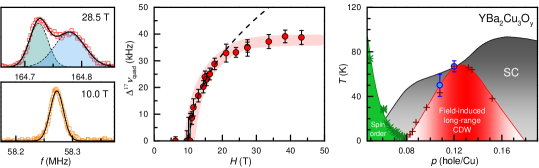
Figure 5: (Color online) NMR evidence for Field Induced Charge density Wave in YBa₂Cu₃O_6+y. Left panels: Splitting of the ¹⁷O NMR line at $T\simeq 2$ K [Tao2013, ]. Middle panel: Field dependence of the quadrupole part of the ¹⁷O line splitting [Tao2013, ]. The dashed line represents a $\sqrt{H-H_{charge}}$ behavior close to the onset field $H_{charge}$. Right panel: Revised phase diagram of YBa₂Cu₃O_y, including the high field CDW from ref. [Tao2011, ]. Crosses correspond to the sign change of the Hall effect and the blue points mark the temperature onset of the NMR splitting.

The relationship between the field-induced CDW, observed by NMR [Tao2011, ; Tao2013, ] and sound velocity measurements [LeBoeuf2013, ], and the zero-field short-range CDW, observed by X-rays [Comin2016, ] and NMR [Tao2015, ], has puzzled the community for a while. However, the presence of two distinct, albeit obviously related, CDW phases was eventually accepted when field-induced long-range CDW was confirmed by X-ray experiments in high magnetic fields [Xraypulsedfields, ; Chang2016, ; Jang2016, ]. These experiments showed that the CDW is indeed of single-$Q$ type, but along the $b$ axis and incommensurate. They also showed that the NMR threshold field corresponds to a growth of the correlation length $\xi_{\textrm{CDW}}$ in the CuO₂ planes. Basically, $\xi_{\textrm{CDW}}$ becomes large enough to produce an NMR pattern –the histogram of the frequency distribution due to the charge modulation– typical of a single $Q$ CDW [Blinc81, ; Butaud1995, ]. On the other hand, the thermodynamic transition observed by the ultrasound technique [LeBoeuf2013, ] occurs at slightly higher field (and, presumably, a slightly lower temperature for the same field), marking the onset of coherence along the $c$ axis. The observation of a 2D pattern in NMR does not require phase coherence along the $c$-axis, as long as the phase fluctuations in the planes are pinned. The long-range CDW phase stacks in-phase along $c$, while the short-range CDW stacks out-of-phase. Both NMR and X-rays find that short-range correlations remain within the long-range phase [Tao2015, ; Xraypulsedfields, ; Chang2016, ; Jang2016, ]. This is likely related to the presence of disorder [Tao2015, ; Jang2016, ; Julien15, ].

Addressing all the recent developments related to CDW order in the cuprates is beyond the scope of this short review on high-field NMR (see refs. [HTCReview, ; Comin2016, ; Julien15, ; PDW, ] for recent perspectives). Let us only mention here the discovery of an intra-unit-cell d-wave symmetry of the CDW as one of the outstanding recent achievements [Fujita14, ; Comin15a, ], showing that this CDW is by no means conventional. Many outstanding questions are still debated, such as whether the Fermi surface is primarily reconstructed by the short-range or the long-range CDW, the role of disorder in shaping the complex phenomenology, and, most importantly, the relationship between CDW and other phenomena in the pseudogap phase (particularly other ordering phenomena) and the relationship with superconductivity. NMR investigation of the field-induced CDW in YBa₂Cu₃O_y is being pursued [Zhou17, ], other systems will be investigated with high-field NMR (see a puzzling recent report in Bi₂Sr_2-xLa_xCuO_6+δ [Kawasaki17, ]) and it is both desirable and likely that other techniques like Raman scattering and optical spectroscopy will provide new insights upon going to high fields. Clearly, this research area will benefit from further development of experiments in, always higher, pulsed and steady magnetic fields.

V Exotic superconductivity

V.1 FFLO state in $\kappa$-(BEDT-TTF)₂Cu(SCN)₂

The Fulde-Ferrell-Larkin-Ovchinikov (FFLO) [Fulde, ; Larkin, ] state is expected to occur in the vicinity of the upper critical field ($H_{\textrm{c2}}$) when Pauli pair breaking dominates over orbital effects [Maki, ; Gruenberg, ]. Pauli pair breaking prevails in fields for which the Zeeman energy is strong enough to break the Cooper pair by flipping one spin of the singlet. In a FFLO state, the Copper pairs acquire a finite momentum, leading to a modulated superconducting state, which can be schematised as periodically alternating “superconducting” and “normal” regions. In solid state physics, the search for FFLO state has been mainly focused on the heavy fermion compound CeCoIn₅ [Bianchi03, ; Koutroulakis10, ] and layered organic superconductors [Singleton00, ; Lortz07, ; Bergk11, ; Uji06, ]. In the case of CeCoIn₅, the phase initially identified as an FFLO one has been shown to be magnetically ordered [Young2007, ; Kenzelman2008, ], and the putative coexistence with an FFLO state is still a matter of debate [Koutroulakis10, ; Hatakeyama2015, ; Kim2016, ].

Quasi-2D organic superconductors are indeed ideal systems to observe FFLO state, because of their large anisotropy: when the magnetic field is strictly aligned within the superconducting planes, there are only Josephson vortices [Roditchev, ] left. Thermodynamic measurements have shown in the phase diagram of the compound $\kappa$-(BEDT-TTF)₂Cu(SCN)₂ the existence of a narrow additional superconducting phase just below $H_{\textrm{c2}}$, for $H$ aligned with the conducting plane [Lortz07, ; Bergk11, ; Agosta2012, ; Agosta2016, ], which could be an FFLO phase. The first high-field NMR experiment [Wright, ] was performed at 0.35 K and concluded that the phase transition observed at 21.3 T was Zeeman driven. In spite of efforts to observe directly the spatial modulation of the order parameter, it has not been seen yet. However, it was noted that, due to the modulation of the order parameter, nodes occur forming domain walls in which the superconducting phase changes by $\pi$ [Vorontsov2005, ]. This phase twist leads to a local modification of the density of states and the creation of new topological defects, characterized by the formation of Andreev bound states (ABS), which are a hallmark of the FFLO phase. Recently, a high-field NMR experiment [Mayaffre14, ] has shown that these spin-polarized ABS produce a huge enhancement of the NMR relaxation rate $1/T_{1}$ (Fig 6a), providing the first microscopic characterisation of an FFLO phase. It turns out that this effect only occurs in a limited range of relatively high temperature, which has been consistently explained by theory [Vorontsov2016, ], showing that this enhancement comes from the scattering of electronic spins between the bound and continuum states. A new compound with much smaller $H_{\textrm{c2}}$ values, $\beta$”-(BEDT-TTF)₂SF₅CH₂CF₂SO₃, has been recently investigated [Koutroulakis16, ] by NMR, confirming the nuclear spin-lattice relaxation results obtained in [Mayaffre14, ] are ubiquitous of the FFLO phase, and observing a lineshape compatible with a single-$q$ modulated superconducting phase.

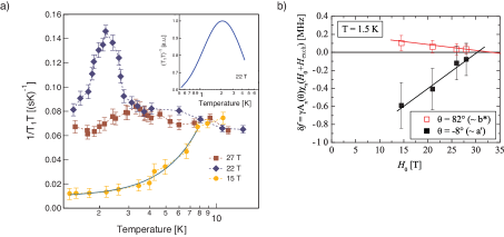
Figure 6: (Color online) (a): NMR relaxation rate in the normal and superconducting states of $\kappa$-(BEDT-TTF)₂Cu(SCN)₂. Temperature dependence of ¹³C NMR $(T_{1}T)^{-1}$ at fields of 15, 22 and 27 T, applied in the conducting planes (symbols). In agreement with the phase diagram based on magnetic torque measurements [Bergk11, ], at 15 T, the system becomes superconductor around 7 K (Solid line denotes the quadratic temperature dependence characteristic for superconductors with a gap having a line of nodes, such as for a $d$-wave symmetry). At 27 T, the system remains normal down to the lowest temperature investigated (1.4 K), while at 22 T, the system enters from the normal state into the FFLO phase. The huge peak in $(T_{1}T)^{-1}$ is due to the Andreev bound states present in the FFLO phase [Mayaffre14, ; Vorontsov2005, ; Vorontsov2016, ]. Inset: Simulation of the $(T_{1}T)^{-1}$ peak due to the Andreev bound states. (b): Field dependence of the spin polarization of the conduction electrons of the $p$-band as measured by ⁷⁷Se NMR (see the text) for two different orientations of the field in the superconducting plane of $\lambda$-(BETS)₂FeCl₄. The two straight lines cross at $H_{0}$ =32 $\pm$ 2 T, when $H_{0}+H_{\textrm{exch}}$ = 0, in agreement with the maximum of $T_{\rm{c}}$ observed at 33 T [Balicas_2001, ].

V.2 Field induced superconductivity in $\lambda$-(BETS)₂FeCl₄

To explain field-induced superconductivity, Jaccarino and Peter [Vincent, ] have proposed a mechanism in which there is a compensation mechanism between the applied magnetic field and the effective negative field seen by the conduction electrons through an exchange mechanism with polarised localised spins. The best realisation of this phenomenon happens in the organic compound $\lambda$-(BETS)₂FeCl₄, which is a charge transfer salt composed of the organic BETS (C₁₀S₄Se₄H₈, bisethylenedithiotetraselenafulvalene) donor molecule and magnetic FeCl₄ (Fe³⁺, $S=5/2$) counter ion [Kobayashi, ]. At $H=0$, the localised Fe spins order below 8 K and the compound becomes insulator. Above 12 T, the AF order is suppressed, the system becomes metallic, and the Fe spins $\mathbf{S}$ are fully polarized at sufficiently low temperature. Increasing $H$ further, a superconducting phase appears at $H=18-20$ T (depending of the orientation of the field) which has to be strictly confined in the $b^{*}$-$c$ BETS conducting plane, thus suppressing the orbital limit [Uji_2001, ]. Because of the presence of the localized spins $\mathbf{S}$, the only technique allowing to measure the polarisation of conduction electrons is NMR. The experiment was performed on a ⁷⁷Se enriched, tiny single crystal of dimensions 3 x 0.05 x 0.01 mm³, placed in an NMR coil of 70 $\mu$m diameter [Hiraki_2007, ]. The Hamiltonian describing the interaction between the nuclear spins $\mathbf{I}^{i}$, the conduction electrons $\mathbf{s}^{k}$ of the conduction band, and the localized spins $\mathbf{S}^{j}$ can be written as

$$\mathcal{H}=\mathcal{H}_{Z}+\mathcal{H}_{Is}+\mathcal{H}_{IS}+\mathcal{H}_{exch}.$$ (14)

The first term is the Zeeman interaction

$$\mathcal{H}_{Z}=\sum_{i}-\gamma\hbar I_{z}^{i}(1+K_{c}^{i})H_{0}+\sum_{j}g_{Fe}\mu_{\rm{B}}S_{z}^{j}H_{0}+\sum_{k}g_{\pi}\mu_{\rm{B}}s_{z}^{k}~{},$$ (15)

in which $K_{c}^{i}$ is the chemical shift, $g_{\pi}$ the $g$ factor for the $\pi$ electron of the conduction band. The second and the third terms are respectively the hyperfine interaction of the $p$-band and the dipolar interaction between the nuclear and the localised Fe spins. This latter can be calculated exactly, taking into account the demagnetisation field. Concerning the last term, experiments were conducted at sufficiently low temperature and high magnetic field so that the magnetisation of the Fe ions was saturated and field independent. $\mathcal{H}_{exch}$ can thus be simply written $\mathcal{H}_{exch}\approx\sum_{k}g_{\pi}\mu_{\rm{B}}s_{z}^{k}H_{exch}$. Finally, the shift from the Larmor frequency, after removal of the dipolar contribution and the chemical shift can be written as

$$\delta f^{i}=f^{i}-\gamma H_{0}=\gamma[A_{\pi}^{i}(\theta)\chi_{\pi}(H_{0}+H_{exch})],$$ (16)

which is a linear function of $H_{0}$. For two different orientations $\theta$, the lines $\delta f$($H_{0}$) cross zero at the same field value (Fig. 6b), allowing the determination of the (negative) value of $H_{exch}=-32\pm 2$ T [Hiraki_2007, ], in excellent agreement with the value of 33 T corresponding to the maximum of $T_{\rm{c}}$  [Balicas_2001, ].

VI Conclusion

In this review paper, we have shown the interest of performing NMR in very high magnetic fields, to explore new field-induced quantum ground states in condensed matter. We have limited ourselves to the case of quantum magnetism, high $T_{\rm{c}}$ superconductors and exotic superconductivity, but many other fields can be considered, like heavy fermions or Dirac electrons for example. There are, of course, some limitations of NMR with respect to other techniques: only nuclei with a sufficient isotopic abundance and suitable gyromagnetic ratio can be studied (although the former constrain can be escaped by isotopic enrichment). On the other hand, tiny samples can be studied, which is not always the case for neutron inelastic scattering. The paper is focused on NMR experiments performed in very high field resistive magnets, but the physics as a function of the magnetic field must be considered as a whole, and the separation between the use of superconducting magnets, resistive magnets, and pulsed magnetic fields is purely technical. In any case, experiments using the two last field sources should be carefully prepared at lower field in superconducting magnets, which are less expensive, and for which the duration of experiments is not limited. We note that fields accessible with superconducting magnets devoted to solid state physics have recently reached 24.6 T [IMR, ]. Obviously, the development of NMR in high magnetic field relies on pushing this limit as high as possible. Up to recently, NMR was the only technique allowing to get microscopic information above 17 T. Nowadays, the development of a dedicated hybrid magnet for neutron scattering provides steady magnetic field up to 27 T, and X-rays scattering under pulsed magnetic field, will allow a fruitful comparison between all these complementary techniques.

References

- (1) C. Berthier, L.P. Lévy, G. Martinez (Eds), High Magnetic Fields. Applications to Condensed Matter Physics and Spectroscopy, Lecture Notes in Physics 595, Springer, Berlin, Heidelberg, New York, 2002.
- (2) P.G. De Gennes, Superconductivity of Metals and Alloys, W.A. Benjamin, New-York, 1966.
- (3) K. von Klitzing, G. Dorda, M. Pepper, Phys. Rev. Lett. 45 (1980) 494.
- (4) D.Tsui, H. Stormer, A. Gossard, Phys. Rev. Lett. 50 (1982) 1599.
- (5) J. Jain, Phys. Rev. Lett. 63 (1989) 199.
- (6) For a review, see D.C. Glattli in Ref.[Cargese, ], p. 1 and R. Shankar, in Ref. [Cargese, ], p. 47.
- (7) S. Gerber et al., Science 350 (2015) 6263.
- (8) For recent information, see https://www.helmholtz-berlin.de/quellen/ber/hfm/index_en.html.
- (9) Y. Fagot-Revurat et al., Phys. Rev. Lett. 77 (1996) 1816.
- (10) Y. Fagot-Revurat et al., Phys. Rev. B 55 (1997) 2964.
- (11) G. Chaboussant et al., Phys. Rev. Lett. 97 (1997) 925.
- (12) G. Chaboussant et al., Eur. Phys. J. B 6 (1998) 167.
- (13) M. Horvatić et al., Phys. Rev. Lett. 83 (1999) 420.
- (14) M.-H Julien et al., Phys. Rev. Lett. 84 (2000) 3422.
- (15) K. Kodama et al., Science 298 (2002) 395.
- (16) M. Horvatić and C. Berthier, in Ref. [Cargese, ] p.191.
- (17) M. Takigawa et al., Phys. B (Amsterdam, Neth.) 346 (2004) 27.
- (18) S. Krämer et al., Phys. Rev. B 76 (2007) 100406(R).
- (19) K. Hiraki et al., J. Phys. Soc. Jpn., Vol. 76 (2007) 124708.
- (20) M. Klanjšek et al., Phys. Rev. Lett. 101 (2008) 137207.
- (21) F. Levy et al., Europhys. Lett. 81 (2008) 67004.
- (22) G. Koutroulakis et al., Phys. Rev. Lett. 104 (2010) 087001.
- (23) T. Wu et al., Nature 477 (2011) 191.
- (24) S. Mukhopadhyay et al., Phys. Rev. Lett. 109 (2012) 177206.
- (25) T. Wu et al., Phys. Rev. B 88 (2013) 014511.
- (26) T. Wu et al., Nat. Commun. 4 (2013) 2113.
- (27) M. Takigawa et al., Phys. Rev. Lett. 110 (2013) 067210.
- (28) S. Krämer et al., Phys. Rev. B 87 (2013) 180405(R).
- (29) M. Jeong et al., Phys. Rev. Lett. 111 (2013) 106404.
- (30) H. Mayaffre et al., , Nature Physics 10 (2014) 928.
- (31) M. Klanjšek et al., Phys. Rev. 92 (2015) 060408(R).
- (32) T. Wu et al., Nature Commun. 6 (2015) 6438.
- (33) M.-H. Julien, Science 350 (2015) 914.
- (34) T. Iye et al., J. Phys. Soc. Jpn. 84 (2015) 043705.
- (35) M. Jeong et al., Phys. Rev. Lett. 117 (2016) 106402.
- (36) R. Blinder et al., Phys. Rev. B 95 (2017) 020404(R).
- (37) A. Orlova et al., Phys. Rev. Lett. 118 (2017) 247201.
- (38) R. Zhou et al., Phys. Rev. Lett. 118 (2017) 017001.
- (39) R. Zhou et al., preprint.
- (40) C.P. Slichter, Principles of Magnetic Resonance, 3rd edn, Springer, Berlin, 1990.
- (41) A. Abragam, Principles of Nuclear Magnetism, Oxford Univ. Press, New York, 1961.
- (42) M. Mehring, V.A. Weberruß, Object-Oriented Magnetic Resonance : Classes and Objects, Calculations and Computations, Academic Press, San Diego, 2001.
- (43) E. Fukushima, S.B.W. Roeder, Experimental Pulse NMR. A nuts and bolts approach, Addison–Wesley, London Amsterdam, 1981.
- (44) A. Narath, in: A. Freeman, R.B. Frankel (Eds.), Hyperfine Interaction, Academic Press, New York London, 1967, p. 287.
- (45) C. Berthier, D. Jérome and P. Molinié, J. Phys.: Solid State Phys. 11 (1978) 797.
- (46) T.D.W. Claridge, High Resolution NMR Techniques in Organic Chemistry, Elsevier, Amsterdam 2016.
- (47) A. Abragam and B. Bleaney, Electronic paramagnetic resonance of transition ions, Clarendon Press, Oxford, 1970.
- (48) J. Winter, Magnetic Resonance in Metals, Clarendon, Oxford, 1971.
- (49) P. Mendels et al., Phys. Rev. Lett. 85 (2000) 3496.
- (50) V.P. Mineev and K.V. Samokhin, Introduction to Unconventional Superconductivity, Gordon and Breach Science Publishers, 1999.
- (51) P. Butaud et al., Phys. Rev. Lett. 55 (1985) 253; P. Butaud et al., J. Phys. France 51 (1990) 59.
- (52) K. Hiraki and K. Kanoda, Phys. Rev. Lett. 80 (1998) 437.
- (53) L.C. Hebel and C.P. Slichter, Phys. Rev. 107 (1957) 901.
- (54) H. Mayaffre et al., Phys. Rev. Lett. 75 (1995) 4122.
- (55) A. Auerbach, Interacting Electrons and Quantum Magnetism, Graduate Text in Contemporay Physics, Springer-Verlag, NewYork, 1994.
- (56) U. Schollwöck, U. J. Richter, D.J.J. Farnell, R.F. Bishop (Eds), Quantum Magnetism, Lect. Notes Phys. 645, Springer, Berlin Heidelberg, 2004.
- (57) T. Giamarchi, Quantum Physics in One Dimension, Clarendon Press, Oxford, 2004.
- (58) S. Sachdev, Quantum Phase Transition, Cambridge University Press, Cambridge, 1998.
- (59) Introduction to Frustration Magnetism, C. Lacroix, P. Mendels, F. Mila (Eds), Springer Series on Solid State Science, Springer, Berlin Heidelberg 2011.
- (60) P. Jordan and E. Wigner, Z. Phys. 47 (1928) 631.
- (61) P.W. Anderson, Science 235 (1987) 1196.
- (62) Magnetized States of Quantum Spin Chains, C. Broholm et al., in Ref. [Cargese, ], pp. 211-234.
- (63) M. Motokawa, H. Ohta, H. Nojiri and S Kimura, J. Phys Soc. Jpn. Vol.72 (2003) Suppl. B pp. 1-11.
- (64) M. Takigawa and F. Mila in Ref. [Frustration_book_2011, ] and references therein.
- (65) T. Giamarchi, C. Rüegg and O. Tchernyshyov, Nat. Phys. 4, (2008) 198.
- (66) V. Zapf, M. Jaime and C.D. Batista, Rev. Mod. Phys. 86 (2014) 563.
- (67) T. Giamarchi and A.M. Tsvelik, Phys. Rev. B 59 (1999) 11398.
- (68) I.E. Dzyaloshinskii, J. Phys. Chem. Solids 4 (1958) 241.
- (69) T. Moriya, Phys. Rev. Lett. 4 (1960) 228.
- (70) L. Balents, Nature 464 (2010) 199.
- (71) T. Nikuni et al., Phys. Rev. Lett. 84 (2000) 5868.
- (72) T.M. Rice, Science 298 (2002) 760.
- (73) F.D.M. Haldane, Phys. Rev. Lett. 45 (1980) 1358.
- (74) S. Kimura et al., Phys. Rev. Lett. 100 (2008) 057202
- (75) S. Kimura et al., PRL 99 (2007) 087602.
- (76) S. Kimura et al., PRL 101 (2008) 207201.
- (77) E. Canévet et al., PRL 87 (2013) 054408.
- (78) B. Grenier et al., Phys. Rev. B 92 (2015) 134416.
- (79) W. Bray et al., The Spin–Peierls Transition, in Extended Linear Compounds, J.C. Miller (Ed) Plenum, New York, 1982, pp. 353.
- (80) M. Hase et al., Phys. Rev. Lett. 70 (1993) 3651 .
- (81) G. Uhrig et al., Phys. Rev. B 60 (1999) 9468.
- (82) H.M. Rønnow et al., Phys. Rev. Lett. 84 (2000) 446.
- (83) K. Kiryhukin et al., Phys. Rev. Lett. 76 (1996) 4608.
- (84) Z. Hiroi et al., J. Solid State Chem. 95 (1991) 230.
- (85) E. Dagotto, Rep. Prog. Phys. 62 (1999) 1571.
- (86) F. Mila, Eur. Phys. J. B 6 (1998) 201.
- (87) T.M. Rice in Ref. [Cargese, ], pp. 139-160.
- (88) F.D.M. Haldane, Phys. Lett. 93A (1983) 464; Phys. Rev. Lett. 50 (1983) 1153.
- (89) M. B. Stone et al., Phys. Rev. B 65 (2002) 064423.
- (90) B. R. Patyal, et al., Phys. Rev. B 41 (1990) 1657.
- (91) B. C. Watson et al., Phys. Rev. Lett. 86 (2001) 5168.
- (92) C. Rüegg et al., Phys. Rev. Lett. 101 (2008) 247202.
- (93) B. Thielemann et al., Phys. Rev. B 79 (2009) 020408(R).
- (94) P. Bouillot et al., Phys. Rev. B 83 (2011) 054407.
- (95) A. Shapiro et al., J. Am. Chem. Soc. 129 (2007) 952.
- (96) T. Hong et al., Phys. Rev. Lett. 105 (2010) 137207.
- (97) D. Schmidiger et al., Phys. Rev. Lett. 108 (2012) 167201.
- (98) M. Enderle et al., Europhys. Lett., 70 (2005) 237.
- (99) T. Hikihara, et al., Phys. Rev. B 78 (2008) 144404.
- (100) J. Sudan, A. Lüscher, and A. M. Läuchli, Phys. Rev. B 80 (2009) 140402.
- (101) M. E. Zhitomirsky and H. Tsunetsugu, Europhys. Lett. 92 (2010) 37001.
- (102) L.E. Svistov et al., JETP Letters 93 (2011) 21.
- (103) N. Büttgen et al., Phys. Rev. B 85 (2012) 214421.
- (104) K. Nawa et al., J. Phys. Soc. Jpn. 82 (2013) 094709.
- (105) N. Büttgen et al., Phys. Rev. B 90 (2014) 134401.
- (106) F. Mila, Physics, 10 (2017) 64.
- (107) A. Smerald and N. Shannon, Phys. Rev. B 93 (2016) 184419.
- (108) B.S. Shastry and B. Sutherland, Physica (Amsterdam) 108B+C (1981) 1069.
- (109) H. Kageyama et al., Phys. Rev. Lett. 82 (1999) 3168.
- (110) A. Koga and N. Kawakami, Phys. Rev. Lett. 84 (2000) 4461.
- (111) P. Corboz and F. Mila, Phys. Rev. B 87 (2013) 115144.
- (112) K. Onizuka et al., J. Phys. Soc. Jpn. 69 (2000) 1016.
- (113) S. E. Sebastian et al., Proc. Natl. Acad. Sci. USA 105 (2008) 20157.
- (114) J. Dorier, K. P. Schmidt, and F. Mila, Phys. Rev. Lett. 101 (2008) 250402.
- (115) A. Abendschein and S. Capponi, Phys. Rev. Lett. 101 (2008) 227201.
- (116) M. Jaime et al., Proc. Natl. Acad. Sci. USA 109 (2012) 12404.
- (117) Y. H. Matsuda et al., Phys. Rev. Lett. 111 (2013) 137204.
- (118) M. Nemec, G. R. Foltin, and K. P. Schmidt, Phys. Rev. B 86 (2012) 174425.
- (119) F. Mila and M. Takigawa, Eur. Phys. J. B 86 (2013) 354.
- (120) P. Corboz and F. Mila, PRL 112 (2014) 147203.
- (121) D.A. Schneider et al., Phys. Rev. B 93 (2016) 241107(R).
- (122) M. E. Zayed et al., Nat. Physics 13 (2017) 962.
- (123) T. Matsubara and H.A. Matsuda, Prog. Theor. Phys. 16 (1956) 569.
- (124) O. Vyaselev et al., Phys. Rev. Lett. 92 (2004) 207202.
- (125) V.S. Zapf et al., Phys. Rev. Lett. 96 (2006) 077204.
- (126) L. Yin et al., PRL 101 (2008) 187205.
- (127) M. Jaime et al., Phys. Rev. Lett. 93 (2004) 087203.
- (128) S.E. Sebastian et al., Nature 441 (2006) 617.
- (129) E.C. Samulon et al., Phys. Rev. B 73 (2006) 100407(R).
- (130) C. Rüegg et al., Phys. Rev. Lett. 98 (2007) 017202.
- (131) O. Rösch and M. Vojta, Phys. Rev. B 76 (2007) 180401(R); 76 (2007) 224408.
- (132) N. Laflorencie and F. Mila, Phys. Rev. Lett. 102 (2009) 037203.
- (133) V.V. Mazurenko et al., Phys. Rev. Lett. 112 (2014) 107202.
- (134) G. Bednorz and K.A. Müller, Z. Phys. B 64 (1986) 189.
- (135) B. Keimer et al., Nature 518 (2015) 179, and references therein.
- (136) H. Alloul, T. Ohno and P. Mendels, Phys. Rev. Lett. 63 (1989) 1700.
- (137) N. Doiron -Leyraud. et al., Nature 447 (2008) 565.
- (138) B. Vignolle et al., C. R. Physique 14 (2013) 39.
- (139) D. LeBoeuf et al., Nature 450 (2007) 533.
- (140) S.E. Sebastian and C. Proust, Annual Review of Condensed Matter Physics 6 (2015) 411.
- (141) J.M. Tranquada et al., Nature 375 (1995) 561.
- (142) R. Comin and A. Damascelli, Annu. Rev. Condens. Matter Phys. 7 (2016) 369.
- (143) G. Grissonnanche et al., Nat. Commun. 5 (2014) 3280.
- (144) G. Ghiringhelli et al., Science 337 ( 2012) 821.
- (145) J. Chang et al., Nature Phys. 8 (2012) 871.
- (146) S. Blanco-Canosa et al., Phys. Rev. B 90 (2014) 054513.
- (147) R. Comin et al., Science 343 (2014) 390.
- (148) E.H. da Silva Neto et al., Science 343 (2014) 393.
- (149) W. Tabis et al., Nature Commun. 5 (2014) 5875.
- (150) K. Ghoshray et al., J. Phys.: Condens. Matter 21 (2009) 155701.
- (151) C. J. Arguello et al., PRB 89 (2014) 235115.
- (152) U. Chatterjee et al., Nat. Phys. 6 (2010) 99.
- (153) M. Le Tacon et al., Nat. Phys. 10 (2014) 52.
- (154) D. LeBoeuf et al., Nature Phys. 9 (2013) 79.
- (155) J. Chang et al., Nature Commun. 7 (2016) 11494.
- (156) H. Jang et al., Proc. Natl. Acad. Sci. USA 113 (2016) 14645.
- (157) R. Blinc, Phys. Reports 79C (1981) 331.
- (158) P. Butaud et al., Phys. Rev. Lett. 55 (1995) 253.
- (159) K. Fujita, et al., Proc. Natl. Acad. Sci. USA 111 (2014) E3026.
- (160) R. Comin et al., Nat. Mater. 14 (2015) 796.
- (161) E. Fradkin, S. A. Kivelson, and J. M. Tranquada, Rev. Mod. Phys. 87 (2015) 457.
- (162) S. Kawasaki et al., arXiv:1704.06169.
- (163) P. Fulde and R. Ferrell, Phys. Rev. 135 (1964) A550.
- (164) A. I. Larkin and Y. N. Ovchinnikov, Sov. Phys. JETP 20 (1965) 762.
- (165) K. Maki, Phys. Rev. 148 (1996) 362.
- (166) L.W. Gruenberg and L. Gunther, Phys. Rev. Lett. 16 (1996) 996.
- (167) A. Bianchi et al., Phys. Rev. Lett. 91 (2003) 187004.
- (168) J. Singleton et al., J. Phys. Condens. Matter 12 (2000) L641.
- (169) R. Lortz et al., Phys. Rev. Lett. 99 (2007) 187002.
- (170) B. Bergk et al., Phys. Rev. B 83 (2011) 064506.
- (171) S. Uji et al., Phys. Rev. Lett. 97 (2006) 157001.
- (172) B.-L. Young et al., Phys. Rev. Lett. 98 036402 (2007).
- (173) M. Kenzelmann et al., Science 321 (2008) 1652.
- (174) Y. Hatakeyama and R. Ikeda, Phys. Rev. B 91 (2015) 94504.
- (175) D. Roditchev et al., Nature Physics 11 (2015) 332.
- (176) Duk.Y. Kim et al., Phys. Rev. X 6 (2016) 041059.
- (177) C. C. Agosta et al., Phys. Rev. B 85 (2012) 214514.
- (178) C.C. Agosta et al., arXiv:1602.06496 (2016).
- (179) J. A. Wright et al., Phys. Rev. Lett. 107 (2011) 087002.
- (180) A.B. Vorontsov, J.A. Saul, and M.J. Graf, Phys. Rev. B 72 (2005) 184501.
- (181) B.M. Rosemeyer and A.B. Vorontsov, Phys. Rev. B 94 (2016) 144501.
- (182) G. Koutroulakis et al., Phys. Rev. Lett. 116 (2016) 067003.
- (183) V. Jaccarino and M. Peter, Phys. Rev. Lett. 9 (1962) 290.
- (184) A. Kobayashi et al., Chem. Lett. 22 (1993) 2179.
- (185) S. Uji et al., Nature 410 (2001) 908.
- (186) L. Balicas et al., Phys. Rev. Lett. 87 (2001) 067002.
- (187) http://www.hflsm.imr.tohoku.ac.jp/cgi-bin/?num=170606115304