Integrable nonlocal Hirota equations

Abstract:

We construct several new integrable systems corresponding to nonlocal versions of the Hirota equation, which is a particular example of higher order nonlinear Schrödinger equations. The integrability of the new models is established by providing their explicit forms of Lax pairs or zero curvature conditions. The two compatibility equations arising in this construction are found to be related to each other either by a parity transformation $\mathcal{P}$, by a time reversal $\mathcal{T}$ or a $\mathcal{PT}$-transformation possibly combined with a conjugation. We construct explicit multi-soliton solutions for these models by employing Hirota’s direct method as well as Darboux-Crum transformations. The nonlocal nature of these models allows for a modification of these solution procedures as the new systems also possess new types of solutions with different parameter dependence and different qualitative behaviour. The multi-soliton solutions are of varied type, being for instance nonlocal in space, nonlocal in time of time crystal type, regular with local structures either in time/space or of rogues wave type.

1 Introduction

The nonlinear Schrödinger equation (NLSE) [1] is a well studied prototypical nonlinear integrable system with many physical applications, most notably in nonlinear optics where it describes the wave propagation in Kerr type media, see e.g. [2], or plasma physics [3]. The main interest in the NLSE arises from the fact that due its integrability it possesses solitonic wave solutions that can be realized in form of optical pulses. While the NLSE provides a very accurate description for the wave propagation of pulses in the picosecond regime [4], experiments in the high-intensity and short pulse subpicosecond, i.e. femtosecond, regime [5, 6] suggested for higher order corrections to be taken into account. Motivated by these physical reasons, Kodama and Hasegawa [7] proposed the higher order nonlinear Schrödinger equation (HNLSE)

$$iq_{t}+\frac{1}{2}q_{xx}+\left|q\right|^{2}q+i\varepsilon\left[\alpha q_{xxx}+\beta\left|q\right|^{2}q_{x}+\gamma q\left|q\right|_{x}^{2}\right]=0,$$ (1)

with constants $\varepsilon,\alpha,\beta,\gamma\in\mathbb{R}$. Besides the NLSE for $\varepsilon=0$, four cases are known to be integrable. When the ratio of the constants are taken to be $\alpha:\beta:\gamma=0:1:1$ or $\alpha:\beta:\gamma=0:1:0$ one obtains the derivative NLSE of type I [8] and II [9], respectively, which are in fact related to each other by a dependent variable transformation [10]. For $\alpha:\beta:\gamma=1:6:3$ one obtains the Sasa-Satsuma equation [11] and for $\alpha:\beta:\gamma=1:6:0$ the Hirota equation [12]. Variations of the latter are the subject of this manuscript.

We notice that the additional term in the HNLSE when compared to the NLSE, i.e. (1) for $\varepsilon=0$, shares the same $\mathcal{PT}$-symmetry with the NLSE, as it is invariant with respect to $\mathcal{PT}:x\rightarrow-x$, $t\rightarrow-t$, $i\rightarrow-i$, $q\rightarrow q$, where $\mathcal{P}:x\rightarrow-x$ and $\mathcal{T}:$ $t\rightarrow-t$, $i\rightarrow-i$. Hence HNLSEs may also be viewed as $\mathcal{PT}$-symmetric extensions of the NLSE. Similarly as for many other $\mathcal{PT}$-symmetric nonlinear integrable systems [13], various other $\mathcal{PT}$-symmetric generalizations have been proposed and investigated by adding terms to the original equation, e.g. [14, 15, 16]. A further option, that will be important here, was explored by Ablowitz and Musslimani [17, 18] who identified a new class of nonlinear integrable systems closely related to the NLSE by exploiting a hitherto unexplored $\mathcal{PT}$-symmetry present in the zero curvature condition. Exploring this option below for the Hirota equation will lead us to new integrable systems with nonlocal properties.

Our manuscript is organized as follows: In section 2 we discuss the zero curvature condition or AKNS-equation for the new class of integrable systems. The solutions to these systems involve fields at different points in space or time and reduce in certain limits to the standard Hirota equation, so that we refer to them as nonlocal Hirota equations. The equations possess two types of solutions of qualitatively different behaviour and parameter dependence. We identify the origin for this novel feature within the context of Hirota’s direct method as well as in the application of Darboux-Crum transformations. At first we discuss these two solution methods for the local Hirota equation in section 3. This will not only serve as a benchmark for what follows, but we will also report new solutions to these equations. In section 4-7 we construct and discuss the solutions for the different types of new models. Our conclusions are stated in section 8.

2 Zero curvature equations for nonlocal Hirota equations

The classical integrability of a model can be established by the Painlevé test [19, 20] or the explicit construction of its Lax pair [21] which is equivalent to the closely related zero curvature condition, also referred to as AKNS-equation [22]. While the former is a mere test, essentially just providing a yes or no answer to the question of whether a model is integrable or not, the latter is more constructive and constitutes a starting point for an explicit solution procedure. The reformulations of the equation of motion of the model in terms of the zero curvature condition allows for the construction of infinitely many conserved charges, which is synonymous to the model being classically integrable. We explore various symmetries in this reformulation that will lead us to new types of models exhibiting novel features.

In general, the zero curvature condition for two operators $U$ and $V$ is equivalent to two linear first order differential equations for an auxiliary function $\Psi$

$$\partial_{t}U-\partial_{x}V+\left[U,V\right]=0\qquad\Leftrightarrow\qquad\Psi_{t}=V\Psi\text{, }\Psi_{x}=U\Psi.$$ (2)

For a concrete model these equation have to hold up to the validity of the equation of motion. When taking the matrix valued functions $U$ and $V$ to be of the general form

$$U=\left(\begin{array}[]{cc}-i\lambda&q(x,t)\\ r(x,t)&i\lambda\end{array}\right),\qquad V=\left(\begin{array}[]{cc}A(x,t)&B(x,t)\\ C(x,t)&-A(x,t)\end{array}\right),\qquad$$ (3)

involving the constant spectral parameter $\lambda$ and at this point arbitrary functions $q(x,t)$ and $r(x,t)$, the zero curvature condition holds when the matrix entries $A$, $B$ and $C$ satisfy the coupled equations

$$A_{x}(x,t) = q(x,t)C(x,t)-r(x,t)B(x,t),$$ (4)

$$B_{x}(x,t) = q_{t}(x,t)-2q(x,t)A(x,t)-2i\lambda B(x,t),$$ (5)

$$C_{x}(x,t) = r_{t}(x,t)+2r(x,t)A(x,t)+2i\lambda C(x,t).$$ (6)

Suppressing now the explicit $x,t$-dependence of the functions involved, a solution to the equations (4)-(6) with arbitrary constants $\alpha$, $\beta$ is

$$A = -i\alpha qr-2i\alpha\lambda^{2}+\beta\left(rq_{x}-qr_{x}-4i\lambda^{3}-2i\lambda qr\right),$$ (7)

$$B = i\alpha q_{x}+2\alpha\lambda q+\beta\left(2q^{2}r-q_{xx}+2i\lambda q_{x}+4\lambda^{2}q\right),$$ (8)

$$C = -i\alpha r_{x}+2\alpha\lambda r+\beta\left(2qr^{2}-r_{xx}-2i\lambda r_{x}+4\lambda^{2}r\right),$$ (9)

when $q(x,t)$ and $r(x,t)$ satisfy the two equations

$$q_{t}-i\alpha q_{xx}+2i\alpha q^{2}r+\beta\left[q_{xxx}-6qrq_{x}\right] = 0,$$ (10)

$$r_{t}+i\alpha r_{xx}-2i\alpha qr^{2}+\beta\left(r_{xxx}-6qrr_{x}\right) = 0.$$ (11)

Next one needs to make sure that these two equations are in fact compatible. Adopting now from [17, 18] the general idea that has been applied to the NLSE to the current setting we explore various choices and alter the $x,t$-dependence in the functions $r$ and $q$. For convenience we suppress the explicit functional dependence and absorb it instead into the function’s name by introducing the abbreviations

$$q:=q(x,t)\text{,\quad}\tilde{q}:=q(-x,t)\text{,\quad}\hat{q}:=q(x,-t)\text{,\quad}\check{q}:=q(-x,-t).\text{\quad}$$ (12)

All six choices for $r(x,t)$ being equal to $\tilde{q}$, $\hat{q}$, $\check{q}$ or their complex conjugates $\tilde{q}^{\ast}$, $\hat{q}^{\ast}$, $\check{q}^{\ast}$ together with some specific adjustments for the constants $\alpha$ and $\beta$ are consistent for the two equations (10) and (11), thus giving rise to six new types of integrable models that have not been explored so far. We will first list them and then study their properties, in particular their solutions, in the next chapters.

The Hirota equation, a conjugate pair, $r(x,t)=\kappa q^{\ast}(x,t)$:

The standard choice to achieve compatibility between (10) and (11) is to take $r(x,t)=\kappa q^{\ast}(x,t)$ with $\kappa=1$. Here we allow $\kappa\in\mathbb{R}$, such that the equations acquire the forms

$$iq_{t} = \!-\alpha\left(q_{xx}-2\kappa\left|q\right|^{2}q\right)\!-i\!\beta\!\left(q_{xxx}-6\kappa\left|q\right|^{2}q_{x}\right),$$ (13)

$$-iq_{t}^{\ast} = -\alpha\left(q_{xx}^{\ast}-2\kappa\left|q\right|^{2}q^{\ast}\right)\!+i\!\beta\!\left(q_{xxx}^{\ast}-6\kappa\left|q\right|^{2}q_{x}^{\ast}\right).\quad\;\;\;\;\;\,$$ (14)

Equation (13) is the known Hirota equation [12]. Taking in (13) $\kappa=1$, $\alpha\rightarrow 1/2$ and $\beta\rightarrow\varepsilon$ we obtain the HNLSE (1) when setting $\alpha\rightarrow 1$, $\beta\rightarrow 6$, $\gamma\rightarrow 0$ in there. For $\alpha,\beta,\kappa\in\mathbb{R}$ equation (14) is its complex conjugate, respectively, i.e. (14)${}^{\ast}=$(13). When $\beta\rightarrow 0$ equation (13) reduces to the NLSE with conjugate (14) and for $\alpha\rightarrow 0$ equation (13) reduces to the complex modified Korteweg de-Vries with conjugate (14). The aforementioned $\mathcal{PT}$-symmetry is preserved in these equations.

A parity transformed conjugate pair, $r(x,t)=\kappa q^{\ast}(-x,t)$:

Taking now $r(x,t)=\kappa\tilde{q}^{\ast}$ with $\kappa\in\mathbb{R}$ together with $\beta=i\delta$, $\alpha,\delta\in\mathbb{R}$, the equations (10) and (11) become

$$\!iq_{t}\! = \!-\alpha\left[q_{xx}-2\kappa\tilde{q}^{\ast}q^{2}\right]\!+\delta\!\left[q_{xxx}-6\kappa q\tilde{q}^{\ast}q_{x}\right],$$ (15)

$$-\!i\tilde{q}_{t}^{\ast} = -\!\alpha\left[\tilde{q}_{xx}^{\ast}-2\kappa q(\tilde{q}^{\ast})^{2}\right]\!-\delta\!\left(\tilde{q}_{xxx}^{\ast}-6\kappa\tilde{q}^{\ast}q\tilde{q}_{x}^{\ast}\right).\quad~{}~{}~{}$$ (16)

We observe that equation (15) is the parity transformed conjugate of equation (16), i.e. $\mathcal{P}$(15)${}^{\ast}=$(16). We also notice that a consequence of the introduction of the nonlocality is that the aforementioned $\mathcal{PT}$-symmetry has been broken.

A time-reversed pair, $r(x,t)=\kappa q^{\ast}(x,-t)$:

Choosing $r(x,t)=\kappa\hat{q}^{\ast}$ with $\kappa\in\mathbb{R}$ and $\alpha=i\hat{\delta}$, $\beta=i\delta$, $\hat{\delta},\delta\in\mathbb{R}$ we obtain from equations (10) and (11) the pair

$$\!iq_{t}\! = \!-i\hat{\delta}\left[q_{xx}-2\kappa\hat{q}^{\ast}q^{2}\right]\!+\delta\!\left[q_{xxx}-6\kappa q\hat{q}^{\ast}q_{x}\right],$$ (17)

$$\!i\hat{q}_{t}^{\ast} = \!i\hat{\delta}\left[\hat{q}_{xx}^{\ast}-2\kappa q(\hat{q}^{\ast})^{2}\right]\!+\delta\!\left(\hat{q}_{xxx}^{\ast}-6\kappa\hat{q}^{\ast}q\hat{q}_{x}^{\ast}\right).\quad~{}~{}~{}$$ (18)

Recalling here that the time-reversal map includes a conjugation, such that $\mathcal{T}:q\rightarrow\hat{q}^{\ast},i\rightarrow-i$, we observe that (17) is the time-reversed of equations (18), i.e. $\mathcal{T}$(18)$=$(17). The $\mathcal{PT}$-symmetry is also broken in this case.

A $\mathcal{PT}$-symmetric pair, $r(x,t)=\kappa q^{\ast}(-x,-t)$:

For the choice $r(x,t)=\kappa\check{q}^{\ast}$ with $\kappa\in\mathbb{R}$ and $\alpha=i\check{\delta}$, $\check{\delta},\beta\in\mathbb{R}$ the equations (10) and (11) become

$$\!q_{t}\! = \!-\check{\delta}\left[q_{xx}-2\kappa\check{q}^{\ast}q^{2}\right]\!-\beta\!\left[q_{xxx}-6\kappa q\check{q}^{\ast}q_{x}\right],$$ (19)

$$\!-\check{q}_{t}^{\ast} = -\!\check{\delta}\left[\check{q}_{xx}^{\ast}-2\kappa q(\check{q}^{\ast})^{2}\right]\!+\beta\!\left(\check{q}_{xxx}^{\ast}-6\kappa\check{q}^{\ast}q\check{q}_{x}^{\ast}\right).\quad~{}~{}~{}$$ (20)

We observe that the overall constant $i$ has cancelled out and the two equations are transformed into each other by means of a $\mathcal{PT}$-symmetry transformation $\mathcal{PT}$(20)$=$(19). Thus, while the $\mathcal{PT}$-symmetry for the equations (19) is broken, the two equations are transformed into each other by that symmetry.

A real parity transformed conjugate pair, $r(x,t)=\kappa q(-x,t)$:

We may also choose $q(x,t)$ to be real. For $r(x,t)=\kappa\tilde{q}$ with $\kappa,\tilde{q}\in\mathbb{R}$ and $\beta=i\delta$, $\alpha,\delta\in\mathbb{R}$, the equations (10) and (11) acquire the forms

$$\!iq_{t}\! = \!-\alpha\left[q_{xx}-2\kappa\tilde{q}q^{2}\right]\!+\delta\!\left[q_{xxx}-6\kappa q\tilde{q}q_{x}\right],$$ (21)

$$\!-i\tilde{q}_{t} = \!-\alpha\left[\tilde{q}_{xx}-2\kappa q\tilde{q}^{2}\right]\!-\delta\!\left(\tilde{q}_{xxx}-6\kappa\tilde{q}q\tilde{q}_{x}\right).\quad~{}~{}~{}$$ (22)

Just as their complex variants (10) and (11), also the equations (22) and (21) are related to each other by conjugation and a parity transformation (16), i.e. $\mathcal{P}$(22)${}^{\ast}=$(21). However, the restriction to real values for $q(x,t)$ makes these equations less interesting as $q$ becomes static, which simply follows from the fact that the left hand sides of (21) and (22) are complex valued, whereas the right hand sides are real valued.

A real time-reversed pair, $r(x,t)=\kappa q(x,-t)$:

For $r(x,t)=\kappa\hat{q}$ with $\kappa,\hat{q}\in\mathbb{R}$ and $\alpha=i\hat{\delta}$, $\beta=i\delta$, $\hat{\delta},\delta\in\mathbb{R}$ we obtain from (10) and (11)

$$\!iq_{t}\! = \!-i\hat{\delta}\left[q_{xx}-2\kappa\hat{q}^{\ast}q^{2}\right]\!+\delta\!\left[q_{xxx}-6\kappa q\hat{q}^{\ast}q_{x}\right],$$ (23)

$$\!\!i\hat{q}_{t}^{\ast} = \!i\hat{\delta}\left[\hat{q}_{xx}^{\ast}-2\kappa q(\hat{q}^{\ast})^{2}\right]\!+\delta\!\left(\hat{q}_{xxx}^{\ast}-6\kappa\hat{q}^{\ast}q\hat{q}_{x}^{\ast}\right).\quad~{}~{}~{}$$ (24)

Again we observe the same behaviour as in the complex variant, namely that the two equations (23) and (24) become their time-reversed counterparts, i.e. $\mathcal{T}$(24)$=$(23). However, as a consequence of $q$ being real these equations simply become the time-reverse NLSE with the additional constraint $q_{xxx}=\pm 6q\hat{q}q_{x}$.

A conjugate $\mathcal{PT}$-symmetric pair, $r(x,t)=\kappa q(-x,-t)$:

For our final choice $r(x,t)=\kappa\check{q}$ we have no restriction on the constants, i.e. $\kappa,\alpha,\beta\in\mathbb{C}$, the equations (10) and (11) become

$$\!q_{t}\! = \!i\alpha\left[q_{xx}-2\kappa\check{q}q^{2}\right]\!-\beta\!\left[q_{xxx}-6\kappa q\check{q}q_{x}\right],$$ (25)

$$\!-\check{q}_{t} = \!i\alpha\left[\check{q}_{xx}-2\kappa q\check{q}^{2}\right]\!+\beta\!\left(\check{q}_{xxx}-6\kappa\check{q}q\check{q}_{x}\right).\quad~{}~{}~{}$$ (26)

These two equations are transformed into each other by means of a $\mathcal{PT}$-symmetry transformation and a conjugation $\mathcal{PT}$(26)${}^{\ast}=$(25). A comment is in order here to avoid confusion. Since a conjugation is included into the $\mathcal{T}$-operator, the additional conjugation of (25) when transformed into (26) means that we simply carry out $x\rightarrow-x$ and $t\rightarrow-t$.

The paired up equations (13)-(26) are all new integrable systems. Let us now discuss solutions and properties of these equations. Since the two equations in each pair are related to each other by a well identified symmetry transformation involving combinations of conjugation, reflections in space and reversal in time, it suffices to focus on just one of the equations.

3 The local Hirota equations, a conjugate pair

Even though the standard Hirota equation [12] and many of its solutions are known, we briefly recall the solution procedure and some of its properties. This will serve as a benchmark that allows us to point out the novelties of the nonlocal equations. We will also report some new solutions. As mentioned, in this case the two equations (10) and (11) are compatible with the choice $r(x,t)=\kappa q^{\ast}(x,t)$.

3.1 Hirota’s direct method

We start by presenting the bilinearisation for the equations (13) and (14), focusing on (13) for the above mentioned reasons. Factorizing the Hirota field as $q(x,t)=g(x,t)/f(x,t)$, with the assumptions $g(x,t)\in\mathbb{C}$, $f(x,t)\in\mathbb{R}$, we find the identify

$$f^{3}\left[iq_{t}+\alpha q_{xx}-2\kappa\alpha\left|q\right|^{2}q+i\!\beta\!\left(q_{xxx}-6\kappa\left|q\right|^{2}q_{x}\right)\right]=$$ (27)

$$f\left[iD_{t}g\cdot f+\alpha D_{x}^{2}g\cdot f+i\beta D_{x}^{3}g\cdot f\right]+\left[3i\beta\left(\frac{g}{f}f_{x}-g_{x}\right)-\alpha g\right]\left[D_{x}^{2}f\cdot f+2\kappa\left|g\right|^{2}\right].~{}~{}~{}$$

The operators $D_{x}$, $D_{t}$ denote the standard Hirota derivatives [23] defined by a Leibniz rule with alternating signs

$$D_{x}^{n}f\cdot g=\sum\limits_{k=0}^{n}\left(\begin{array}[]{l}n\\ k\end{array}\right)(-1)^{k}\frac{\partial^{n-k}}{\partial x^{n-k}}f(x)\frac{\partial^{k}}{\partial x^{k}}g(x).$$ (28)

Here we use the explicit expressions for $D_{t}f\cdot g=f_{t}g-fg_{t}$, $D_{x}^{2}f\cdot g=f_{xx}g-2f_{x}g_{x}+fg_{xx}$ and $D_{x}^{3}f\cdot g=f_{xxx}g-3f_{xx}g_{x}+3f_{x}g_{xx}-fg_{xxx}$. The equation (27) is still trilinear in the functions $f$, $g~{}$and not yet bilinear as required for the applicability of Hirota’s direct method. However, the left hand side vanishes when the Hirota equation (13) holds and the right hand side becomes zero when the two bilinear equations

$$iD_{t}g\cdot f+\alpha D_{x}^{2}g\cdot f+i\beta D_{x}^{3}g\cdot f = 0,$$ (29)

$$D_{x}^{2}f\cdot f = -2\kappa\left|g\right|^{2},$$ (30)

are satisfied. For $\alpha=1/2$ and $\kappa=-1$ they correspond to the equations reported in [24]. When $\beta\rightarrow 0$ the equations (29) and (30) reduce to the bilinear form corresponding to the NLSE [12, 25]. The well known virtue of this formulation is that the bilinear forms can be solved systematically by using the formal power series expansions

$$f(x,t)=\mathop{\displaystyle\sum}\nolimits_{k=0}^{\infty}\varepsilon^{2k}f_{2k}(x,t),\quad\text{and\quad}g(x,t)=\mathop{\displaystyle\sum}\nolimits_{k=1}^{\infty}\varepsilon^{2k-1}g_{2k-1}(x,t).$$ (31)

Solving recursively the equations that result when setting the coefficients of each order in $\varepsilon$ to zero, one obtains different types of solutions corresponding to $n$-soliton solutions with $n$ depending on the order of expansion. A further well known virtue of Hirota’s direct method is the remarkable fact that the quantity $\varepsilon$ is only a formal parameter and can be set to any value. Moreover, despite the fact that initially the Ansatz for the solutions appear to be perturbative, the truncated expansions become exact when setting $f_{k}(x,t)=$ $g_{n}(x,t)=0$ for $k>\ell$, $n>m$, for certain values of $\ell$ and $m$. We will see below that in the nonlocal case we have the new option to weaken this condition which then leads to additional new types of solutions.

In the manner just described the general one-soliton solution can be found by using the truncated expansions $f(x,t)=1+\varepsilon^{2}f_{2}(x,t)$ and $g(x,t)=\varepsilon g_{1}(x,t)$ in (29) and (30). Setting $\varepsilon=1$ without loss of generality, we obtain the local solution

$$q_{\text{l}}^{(1)}(x,t)=\frac{g_{1}(x,t)}{1+f_{2}(x,t)},~{}~{}~{}~{}\ \ \ \ \ \ \text{with \ }g_{1}=\lambda\tau_{\mu,\gamma}\text{,~{}~{}~{}}f_{2}(x,t)=\frac{-\kappa\left|\lambda\right|^{2}}{(\mu+\mu^{\ast})^{2}}\left|\tau_{\mu,\gamma}\right|^{2},$$ (32)

with constants $\mu$,$\gamma$,$\lambda\in\mathbb{C}$ and function

$$\tau_{\mu,\gamma}(x,t):=e^{\mu x+\mu^{2}(i\alpha-\beta\mu)t+\gamma}.$$ (33)

We observe that for real parameter $\alpha$ the presence of the deformation parameter $\beta$ changes drastically the overall qualitative behaviour of the wave. When it is vanishing, that is in the case of the NLSE, the solution is simply a standing wave that changes its amplitude as a function of time. However, when $\beta$ is switched on the solutions of the full Hirota equation displays a qualitatively different behaviour than the one for the NLSE as the wave starts to move with a speed $v=\beta\mu^{2}$.

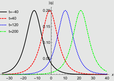
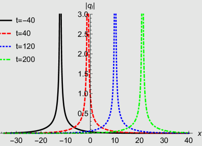
Figure 1: Regular and singular one-soliton solutions (32) for the local Hirota equations (13) at different times for $\alpha=0.5$, $\beta=0.7$, $\gamma=0.4+i0.3$, $\mu=0.2+i0.3$, $\lambda=1$ for $\kappa=-1$ and $\kappa=1$ in the left and right panel, respectively.

From figure 1 we also observe that for $\kappa=1$ the solution (32) develops a singularity. Even though these cusp solutions have possible applications [26] and are interesting in their own right, we will often just focus on the equation for $\kappa=-1$ in what follows, since apart from the overall sign the actual value of $\kappa$ is irrelevant as it can be absorbed into $\lambda$.

To obtain the two-soliton solution we need to go two orders further in the expansion (31) and use $f(x,t)=1+\varepsilon^{2}f_{2}(x,t)+\varepsilon^{4}f_{4}(x,t)$, $g(x,t)=\varepsilon g_{1}(x,t)+\varepsilon^{3}g_{3}(x,t)$ in the bilinear equations (29), (30). Setting $\varepsilon=1$ we obtain the two-soliton solution

$$q_{\text{l}}^{(2)}(x,t)=\frac{g_{1}(x,t)+g_{3}(x,t)}{1+f_{2}(x,t)+f_{4}(x,t)}$$ (34)

with

$$g_{1} = \tau_{\mu,\gamma}+\tau_{\nu,\delta},$$ (35)

$$g_{3} = \frac{\left(\mu-\nu\right)^{2}}{\left(\mu+\mu^{\ast}\right)^{2}\left(\nu+\mu^{\ast}\right)^{2}}\tau_{\nu,\delta}\left|\tau_{\mu,\gamma}\right|^{2}+\frac{\left(\mu-\nu\right)^{2}}{\left(\mu+\nu^{\ast}\right)^{2}\left(\nu+\nu^{\ast}\right)^{2}}\tau_{\mu,\gamma}\left|\tau_{\nu,\delta}\right|^{2},$$ (36)

$$f_{2} = \frac{\left|\tau_{\mu,\gamma}\right|^{2}}{\left(\mu+\mu^{\ast}\right)^{2}}+\frac{\tau_{\nu,\delta}\tau_{\mu,\gamma}^{\ast}}{\left(\nu+\mu^{\ast}\right)^{2}}+\frac{\tau_{\mu,\gamma}\tau_{\nu,\delta}^{\ast}}{\left(\mu+\nu^{\ast}\right)^{2}}+\frac{\left|\tau_{\nu,\delta}\right|^{2}}{\left(\nu+\nu^{\ast}\right)^{2}},$$ (37)

$$f_{4} = \frac{\left(\mu-\nu\right)^{2}\left(\mu^{\ast}-\nu^{\ast}\right)^{2}}{\left(\mu+\mu^{\ast}\right)^{2}\left(\nu+\mu^{\ast}\right)^{2}\left(\mu+\nu^{\ast}\right)^{2}\left(\nu+\nu^{\ast}\right)^{2}}\left|\tau_{\mu,\gamma}\right|^{2}\left|\tau_{\nu,\delta}\right|^{2}.$$ (38)

In comparison with the NLSE the Hirota equation exhibits a more varied behaviour due to the presence of the additional parameter $\beta$. In figure 2 we display a two-soliton composed of a fast one-soliton overtaking a slower one. For a complex choice of the spectral and shift parameter this behaviour is changed into a head-on collision of two one-solitons.

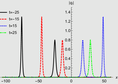
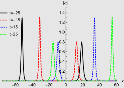
Figure 2: Modulus of the two-soliton solutions (34) for the local Hirota equations (13) at different times for $\alpha=0.4$, $\beta=1.8$, $\gamma=0.3$, $\delta=0.4$, $\mu=1.3$, $\nu=0.8$, $\lambda=1$, $\kappa=-1$ displaying a faster soliton overtaking a slower one (left panel) and $\gamma=0.3+i0.1$, $\delta=0.4+i0.7$, $\mu=1.3+i0.5$, $\nu=0.8+i0.65$, $\lambda=1$, $\kappa=1$ displaying a head-on collision (right panel).

More striking is the previously not pointed out possibility that within the two-soliton solution one of the one-solitons contributions can be made static by a suitable parameter choice. We observe in figure 3 that the static soliton can be seen as a defect. The only effect of the scattering is the usual slight displacement or time-delay depending on the reference frame.

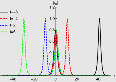
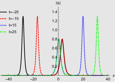
Figure 3: Modulus of the two-soliton solutions (34) for the local Hirota equations (13) at different times for $\alpha=0.4$, $\beta=0.8$, $\gamma=0.3+i0.1$, $\delta=0.4+i0.7$, $\lambda=1$, $\kappa=-1$ with a left moving one-soliton with $\mu=1.-i1.4$, $\nu=0.8+i0.65$ (left panel) and a right moving one-soliton with $\mu=1.3+i0.5$, $\nu=0.8+i0.65$, (right panel) scattering with a static one-solition acting as a defect.

3.2 Darboux-Crum transformations

Alternatively, the solutions of the Hirota equation can also be constructed following the Darboux-Crum transformation scheme [27, 28, 29]. At first we will keep our discussion very general by leaving the functions $q$ and $r$ generic without specifying the different choices for $r$ and consider those concrete scenarios in the next sections.

Generally speaking, Darboux transformations relate two different Hamiltonian systems by means of an intertwining relation [27, 28, 29]. The iteration of this procedure to a sequence of Hamiltonian systems is usually referred to as the Darboux-Crum transformation scheme. In the present case we can convert one of the AKNS equations into an eigenvalue equation and thus identify a Hamiltonian of Dirac type. Taking $\Psi$ to be a two-dimensional vector we obtain

$$\Psi=\left(\begin{array}[]{c}\varphi\\ \phi\end{array}\right),~{}~{}~{}~{}~{}~{}\quad\Psi_{x}=U\Psi~{}\implies\quad\begin{array}[]{c}-i\varphi_{x}+iq\phi=-\lambda\varphi\\ i\phi_{x}-ir\varphi=-\lambda\phi\end{array}\,.$$ (39)

Comparing with the eigenvalue equation $H\Psi(\lambda)=-\lambda\Psi(\lambda)$, we read off the Hamiltonian

$$H=\left(\begin{array}[]{cc}-i\partial_{x}&iq\\ -ir&i\partial_{x}\end{array}\right)\,=-i\sigma_{3}\partial_{x}+V,$$ (40)

from (39), with $\sigma_{3}$ denoting a standard Pauli matrix. Next we seek to relate this Hamiltonian, together with its eigenfunctions, to a set of new Hamiltonians of similar structure

$$H_{n}=\left(\begin{array}[]{cc}-i\partial_{x}&iq_{n}\\ -ir_{n}&i\partial_{x}\end{array}\right)\,=-i\sigma_{3}\partial_{x}+V_{n},$$ (41)

satisfying $H_{n}\Psi_{n}(\lambda)=-\lambda\Psi_{n}(\lambda)$ for $n\in\mathbb{N}$. By construction the new Hamiltonians are designed in such a way that the $q_{n}$ and $r_{n}$ satisfy the two equations resulting from the zero curvature condition with spectral parameters $\lambda_{n}$ and are therefore also solutions to our nonlinear wave equations. Let us next discuss how to obtain them by employing the Darboux-Crum transformation scheme for Dirac Hamiltonians as discussed in [30, 31]. The key assumption is that the different Hamiltonians are recursively related to each other by intertwining relations

$$L_{n}H_{n-1}=H_{n}L_{n},$$ (42)

with intertwining operators $L_{n}$. Identifying $H_{0}=H$, the iteration of the equations (42) lead to the relation $\mathcal{L}_{n}H=H_{n}\mathcal{L}_{n}$ with $\mathcal{L}_{n}:=L_{n}L_{n-1}\ldots L_{1}$. It is also easily verified that the wavefunctions at each level of iteration are simply $\Psi_{n}(\lambda)=\mathcal{L}_{n}\Psi(\lambda)$.

Next we discuss how to obtain the intertwining operators and the potentials. We start with equation (42) for $n=1$ and assume the intertwining operator to be of the general form $L_{1}:=$ $\mathbb{I}\partial_{x}+B$. Upon substituting $H,H_{1}$ and $L_{1}$the intertwining relation yields the two equations

$$V_{1}=V-i\left[B,\sigma_{3}\right],\qquad\text{and\qquad}V_{x}+BV-V_{1}B+i\sigma_{3}B_{x}=0.$$ (43)

Taking next $B=-U_{x}U^{-1}$, as suggested in [30], and substituting the first equation in (43) into the second, the latter becomes equivalent to

$$\left(U^{-1}HU\right)_{x}=0.$$ (44)

Integrating this equation leads to $HU=U\Lambda$ with $\Lambda$ containing the integration constants. This equation has now become formally equivalent to the Schrödinger equation with the difference that $U$ is a matrix. Taking $\mathop{\mathrm{d}iag}\Lambda=(-\lambda_{1},-\lambda_{2})$ this equation is solved by $U=\left(\Psi(\lambda_{1}),\Psi(\lambda_{2})\right)=:U_{1}$ and thus we have found

$$L_{1}=\mathbb{I}\partial_{x}-\left(U_{1}\right)_{x}U_{1}^{-1}\qquad\text{and\qquad}V_{1}=V+i\left[\left(U_{1}\right)_{x}U_{1}^{-1},\sigma_{3}\right].$$ (45)

We may now simply iterate these equations obtaining

$$\begin{array}[]{lll}U_{2}=\left(L_{1}\Psi(\lambda_{3}),L_{1}\Psi(\lambda_{4})\right),{}{}&L_{2}=\mathbb{I}\partial_{x}-\left(U_{2}\right)_{x}U_{2}^{-1},{}{}&V_{2}=V_{1}+i\left[\left(U_{2}\right)_{x}U_{2}^{-1},\sigma_{3}\right],\\ U_{3}=\left(L_{2}L_{1}\Psi(\lambda_{5}),L_{2}L_{1}\Psi(\lambda_{6})\right),&L_{3}=\mathbb{I}\partial_{x}-\left(U_{3}\right)_{x}U_{3}^{-1},&V_{3}=V_{2}+i\left[\left(U_{3}\right)_{x}U_{3}^{-1},\sigma_{3}\right],\\ ~{}~{}~{}~{}~{}\ \ \ \ \ \ ~{}~{}~{}~{}~{}\ \ \ \ \ \ \ \ \ \ \vdots&~{}\ \ \ \ \ \ \ \ \ \ \ \ \ \ \vdots&~{}~{}\ \ \ \ \ \ \ \ \ \ \ \ \ \ \ \ \ \ \ \vdots\\ U_{n}=\left(\mathcal{L}_{n}\Psi(\lambda_{2n-1}),\mathcal{L}_{n}\Psi(\lambda_{2n})\right),&L_{n}=\mathbb{I}\partial_{x}-\left(U_{n}\right)_{x}U_{n}^{-1},&V_{n}=V_{n-1}+i\left[\left(U_{n}\right)_{x}U_{n}^{-1},\sigma_{3}\right].\end{array}$$ (46)

What is left is to specify our original solution $\Psi(\lambda)$. Adopting the notation from [31], we abbreviate $\Omega_{i}=\Psi(\lambda_{i})$ so that at level $n$ of the iteration procedure we have a set of $2n$ spinors that can be viewed as null states for the intertwining operator $\mathcal{L}_{n}$

$$S_{2n}=\left\{\Omega_{1},\Omega_{2},\ldots,\Omega_{2n-1},\Omega_{2n}\right\},\qquad\Omega_{i}=\left(\begin{array}[]{c}\varphi_{i}\\ \phi_{i}\end{array}\right),\quad\lambda_{i}\neq\lambda_{j},$$ (47)

i.e. we have $\mathcal{L}_{n}\Omega_{i}=0$ for $i=1,...,2n$.

Having in principle computed $V_{n}$ in an iterative manner, as in indicated (46), we just need to read off the off-diagonal elements to identify the new solutions $q_{n}$ and $r_{n}$, because the Darboux-Crum scheme guarantees that they satisfy the equations (10) and (11) when $q$ and $r$ are solutions. These expressions constitute the multi-soliton solutions we are seeking to construct.

To be explicit, in the first iteration step we have

$$L_{1}=\mathbb{I}\partial_{x}+\frac{1}{\det W_{1}}\left(\begin{array}[]{cc}\det D_{1}^{1}&-\det D_{1}^{q}\\ \det D_{1}^{r}&\det D_{1}^{2}\end{array}\right),~{}V_{1}=V_{0}+\frac{2i}{\det W_{1}}\left(\begin{array}[]{cc}0&\det D_{1}^{q}\\ \det D_{1}^{r}&0\end{array}\right),$$ (48)

where we introduced the matrices

$$W_{1}=\left(\begin{array}[]{cc}\varphi_{1}&\phi_{1}\\ \varphi_{2}&\phi_{2}\end{array}\right),~{}D_{1}^{q}=\left(\begin{array}[]{cc}\varphi_{1}^{\prime}&\varphi_{1}\\ \varphi_{2}^{\prime}&\varphi_{2}\end{array}\right),~{}D_{1}^{r}=\left(\begin{array}[]{cc}\phi_{1}^{\prime}&\phi_{1}\\ \phi_{2}^{\prime}&\phi_{2}\end{array}\right),~{}D_{1}^{1}=\left(\begin{array}[]{cc}\varphi_{1}^{\prime}&\phi_{1}\\ \varphi_{2}^{\prime}&\phi_{2}\end{array}\right),~{}D_{1}^{2}=\left(\begin{array}[]{cc}\varphi_{1}&\phi_{1}^{\prime}\\ \varphi_{2}&\phi_{2}^{\prime}\end{array}\right).$$ (49)

From $V_{1}$ we read off the one-soliton solution

$$q_{1}=q+2\frac{\varphi_{1}^{\prime}\varphi_{2}-\varphi_{1}\varphi_{2}^{\prime}}{\varphi_{1}\phi_{2}-\varphi_{2}\phi_{1}}\,,\qquad\text{and\qquad}r_{1}=r-2\frac{\phi_{1}^{\prime}\phi_{2}-\phi_{1}\phi_{2}^{\prime}}{\varphi_{1}\phi_{2}-\varphi_{2}\phi_{1}}.$$ (50)

In a similar fashion we can use now (46) to compute iteratively the higher order solutions. Remarkably the $n$-solition solutions can be presented in a closed compact form as

$$q_{n}=q+2\frac{\det D_{n}^{q}}{\det W_{n}}\,,\qquad\text{and\qquad}r_{n}=r-2\frac{\det D_{n}^{r}}{\det W_{n}},$$ (51)

with $W_{n}$, $D_{n}^{q}$ and $D_{n}^{r}$ denoting $2n\times 2n$-matrices generalizing (49). The determinant of the matrix $W_{n}$ corresponds to the generalized Wronskian of the set in (47) with $n$ columns containing $\varphi_{i}$, $i=1,...,2n$, and its derivatives and $n$ columns containing $\phi_{i}$ and its derivatives with respect to $x$

$$W_{n}=\left(\begin{array}[]{cccccccc}\varphi_{1}^{(n-1)}&\varphi_{1}^{(n-2)}&\ldots&\varphi_{1}&\phi_{1}^{(n-1)}&\ldots&\phi_{1}^{\,\prime}&\phi_{1}\\ \varphi_{2}^{(n-1)}&\varphi_{2}^{(n-2)}&\ldots&\varphi_{2}&\phi_{2}^{(n-1)}&\ldots&\phi_{2}^{\,\prime}&\phi_{2}\\ \vdots&\vdots&\ddots&\vdots&\vdots&\ddots&\vdots&\vdots\\ \varphi_{2n}^{(n-1)}&\varphi_{2n}^{(n-2)}&\ldots&\varphi_{2n}&\phi_{2n}^{(n-1)}&\ldots&\phi_{2n}^{\,\prime}&\phi_{2n}\end{array}\right).$$ (52)

The matrix $D_{n}^{q}$ is made up of $n-1$ columns containing $\varphi_{i}$ and its derivatives and $n+1$ columns containing $\phi_{i}$ and its derivatives

$$D_{n}^{q}=\left(\begin{array}[]{cccccccc}\phi_{1}^{(n-2)}&\phi_{1}^{(n-3)}&\ldots&\phi_{1}&\varphi_{1}^{(n)}&\ldots&\varphi_{1}^{\,\prime}&\varphi_{1}\\ \phi_{2}^{(n-2)}&\phi_{2}^{(n-3)}&\ldots&\phi_{2}&\varphi_{2}^{(n)}&\ldots&\varphi_{2}^{\,\prime}&\varphi_{2}\\ \vdots&\vdots&\ddots&\vdots&\vdots&\ddots&\vdots&\vdots\\ \phi_{2n}^{(n-2)}&\phi_{2n}^{(n-3)}&\ldots&\phi_{2n}&\varphi_{2n}^{(n)}&\ldots&\varphi_{2n}^{\,\prime}&\varphi_{2n}\end{array}\right),$$ (53)

and the matrix $D_{n}^{r}$ is made up of $n+1$ columns containing $\varphi_{i}$ and its derivatives and $n-1$ columns containing $\phi_{i}$ and its derivatives

$$D_{n}^{r}=\left(\begin{array}[]{cccccccc}\phi_{1}^{(n)}&\phi_{1}^{(n-1)}&\ldots&\phi_{1}&\varphi_{1}^{(n-2)}&\ldots&\varphi_{1}^{\,\prime}&\varphi_{1}\\ \phi_{2}^{(n)}&\phi_{2}^{(n-1)}&\ldots&\phi_{2}&\varphi_{2}^{(n-2)}&\ldots&\varphi_{2}^{\,\prime}&\varphi_{2}\\ \vdots&\vdots&\ddots&\vdots&\vdots&\ddots&\vdots&\vdots\\ \phi_{2n}^{(n)}&\phi_{2n}^{(n-1)}&\ldots&\phi_{2n}&\varphi_{2n}^{(n-2)}&\ldots&\varphi_{2n}^{\,\prime}&\varphi_{2n}\end{array}\right).$$ (54)

Thus we obtain the $2$-soliton solution from $W_{2}$, $D_{2}^{r}$ and $D_{2}^{r}$, the $3$-soliton solution from $W_{3}$, $D_{3}^{r}$ and $D_{3}^{r}$, etc. A closed expression for the $\mathcal{L}_{n}$-operator can be found in [31].

Let us now construct some concrete solutions. First we need to determine $\Psi_{1}$ by solving (2). Specifying the “seed functions” $q$ and $r$ as $r(x,t)=q(x,t)=0$, taking $\lambda\rightarrow i\lambda$ the component equations for the two linear equations $\left(\Psi_{1}\right)_{t}=V\Psi_{1}$ and $\left(\Psi_{1}\right)_{x}=U\Psi_{1}$ in (2) decouple into

$$\left(\varphi_{1}\right)_{x}=\lambda\varphi_{1},~{}~{}\left(\phi_{1}\right)_{x}=-\lambda\phi_{1},~{}~{}\left(\varphi_{1}\right)_{t}=2\lambda^{2}(i\alpha-2\beta\lambda)\varphi_{1},~{}~{}\left(\phi_{1}\right)_{t}=-2\lambda^{2}(i\alpha-2\beta\lambda)\phi_{1}.$$ (55)

These equations are easily solved by

$$\Psi_{1}(x,t;\lambda)=\left(\begin{array}[]{c}\varphi_{1}(x,t;\lambda)\\ \phi_{1}(x,t;\lambda)\end{array}\right)=\left(\begin{array}[]{c}e^{\lambda x+2\lambda^{2}(i\alpha-2\beta\lambda)t+\gamma_{1}}\\ e^{-\lambda x-2\lambda^{2}(i\alpha-2\beta\lambda)t+\gamma_{2}}\end{array}\right),$$ (56)

with constants $\gamma_{1}$,$\gamma_{2}\in\mathbb{C}$. Next we implement the constraint $r(x,t)=\kappa q^{\ast}(x,t)$, that converts the local Hirota equation (13) into its conjugate (14). Given the solution (50) for $r=q=0$ this restriction leads to $\varphi_{2}=\phi_{1}^{\ast}$, $\phi_{2}=\kappa\varphi_{1}^{\ast}$, so that

$$\!\Psi_{2}(x,t;\lambda)=\left(\begin{array}[]{c}\varphi_{2}(x,t;\lambda)\\ \phi_{2}(x,t;\lambda)\end{array}\right)=\left(\begin{array}[]{c}\phi_{1}^{\ast}(x,t;\lambda)\\ \kappa\varphi_{1}^{\ast}(x,t;\lambda)\end{array}\right)=\left(\begin{array}[]{c}e^{-\lambda^{\ast}x+2t({\lambda^{\ast})}^{2}(i\alpha+2\beta\lambda^{\ast})+\gamma_{2}^{\ast}}\\ \kappa e^{\lambda^{\ast}x-2t({\lambda^{\ast})}^{2}(i\alpha+2\beta\lambda^{\ast})+\gamma_{1}^{\ast}}\end{array}\right).$$ (57)

Substituting these expressions into (50) we obtain the one-soliton solution

$$q_{1}(x,t)=-\frac{2(\lambda+\lambda^{\ast})e^{2\lambda x+4\lambda^{2}t\left(i\alpha-2\beta\lambda\right)+\gamma_{1}-\gamma_{2}}}{1-\kappa e^{2(\lambda+\lambda^{\ast})x+4i\alpha(\lambda^{2}-({\lambda^{\ast})}^{2})t-8\beta(\lambda^{3}+({\lambda^{\ast})}^{3})t+\gamma_{1}+\gamma_{1}^{\ast}-\gamma_{2}-\gamma_{2}^{\ast}}}.$$ (58)

This solution agrees exactly with the one obtained by means of Hirota’s method in (32) when we set in there $\lambda\rightarrow 2(\lambda+\lambda^{\ast})$, $\mu\rightarrow 2\lambda$, $\gamma\rightarrow\gamma_{1}-\gamma_{2}$, $\kappa\rightarrow 1$.

In the same way we can construct a $n$-soliton solutions using the set

$$\tilde{S}_{2n}=\left\{\Psi_{1}(x,t;\lambda_{1}),\Psi_{2}(x,t;\lambda_{1}),\Psi_{1}(x,t;\lambda_{2}),\Psi_{2}(x,t;\lambda_{2}),...,\Psi_{1}(x,t;\lambda_{n}),\Psi_{2}(x,t;\lambda_{n})\right\}$$ (59)

with $\lambda_{i}\neq\lambda_{j}$ in the evaluation of the formulae (51). As we shall discuss below, the solutions to the new non-local equations are obtained by keeping the same seeds in the constructions of the wavefunctions $\Psi_{1}$ and by implementing different types of constraints in the construction of $\Psi_{2}$.

We conclude with a remark on how to obtain degenerate solutions for the cases with equal eigenvalues as discussed in detail for other models in [32, 33, 34]. Instead of considering the set (47) with $\Omega_{i}$ provided $\lambda_{i}\neq\lambda_{j}$, we need to implement Jordan states and use the set

$$\widetilde{S}_{2n}^{\text{deg}}=\left\{\Omega_{1},\Omega_{2},\partial_{\lambda}\Omega_{1},\partial_{\lambda}\Omega_{2},\ldots,\partial_{\lambda}^{n-1}\Omega_{1},\partial_{\lambda}^{n-1}\Omega_{2}\right\},~{}\Omega_{1}=\left(\begin{array}[]{c}\varphi_{1}\\ \phi_{1}\end{array}\right),\Omega_{2}=\left(\begin{array}[]{c}\varphi_{2}\\ \phi_{2}\end{array}\right)\,.$$ (60)

in the evaluation of the formulae (51). Obviously, the combinations of the two different kind of seeds are also possible giving rise to new building blocks ${\tilde{S}}_{2n}$ and $\widetilde{S}_{2n}^{\text{deg}}$.

4 The nonlocal complex parity transformed Hirota equation

In this case the compatibility between the equation (10) and (11) is achieved by the choice $r(x,t)=\kappa q^{\ast}(-x,t)$. As $x$ is now directly related to $-x$, we expect some nonlocality in space to emerge in this model.

4.1 Hirota’s direct method

Let us now consider the new nonlocal integrable equation (15) for $\kappa=-1$. We factorize again $q(x,t)=g(x,t)/f(x,t)$, but unlike as in the local case we no longer assume $f(x,t)$ to be real but allow $g(x,t),f(x,t)\in\mathbb{C}$. We then find the identity

$$f^{3}\tilde{f}^{\ast}\left[iq_{t}\!+\alpha q_{xx}+2\alpha\tilde{q}^{\ast}q^{2}-\delta\!\left(q_{xxx}+6q\tilde{q}^{\ast}q_{x}\right)\right]=$$ (61)

$$f\tilde{f}^{\ast}\left[iD_{t}g\cdot f+\alpha D_{x}^{2}g\cdot f-\delta D_{x}^{3}g\cdot f\right]+\left(\tilde{f}^{\ast}D_{x}^{2}f\cdot f-2fg\tilde{g}^{\ast}\right)\left(\frac{3\delta}{f}D_{x}g\cdot f-\alpha g\right).$$

When comparing with the corresponding identity in the local case (27), we notice that this equation is of higher order in the functions involved, in this case $g$,$\tilde{g}^{\ast}$,$f$,$\tilde{f}^{\ast}$, having increased from three to four. The left hand side vanishes when the local Hirota equation (15) holds and the right hand side vanishes when demanding

$$iD_{t}g\cdot f+\alpha D_{x}^{2}g\cdot f-\delta D_{x}^{3}g\cdot f=0,$$ (62)

together with

$$\tilde{f}^{\ast}D_{x}^{2}f\cdot f=2fg\tilde{g}^{\ast}.$$ (63)

We notice that equation (63) is still trilinear. However, it may be bilinearised by introducing the auxiliary function $h(x,t)$ and requiring the two equations

$$D_{x}^{2}f\cdot f=hg,\qquad\text{and\qquad}2f\tilde{g}^{\ast}=h\tilde{f}^{\ast},$$ (64)

to be satisfied separately. In this way we have obtained a set of three bilinear equations (62) and (64) instead of two. These equations may be solved systematically by using in addition to (31) the formal power series expansion

$$h(x,t)=\mathop{\displaystyle\sum}\nolimits_{k}\varepsilon^{k}h_{k}(x,t).$$ (65)

For vanishing deformation parameter $\delta\rightarrow 0$ the equations (62) and (64) constitute the bilinearisation for the nonlocal NLSE. As our equation differ from the ones recently proposed for that model in [35] we will comment below on some solutions related to that specific case. The local equations presented in the previous section are obtained for $\tilde{f}^{\ast}\rightarrow f$, $\tilde{g}\rightarrow g$, $h\rightarrow g^{\ast}$ as in this case the two equations in (64) combine into the one equation (30).

4.1.1 Two types of one-soliton solutions

Let us now solve the bilinear equations (62) and (64). First we construct the one-soliton solutions. Unlike as in the local case we have here several options, obtaining different types. Using the truncated expansions

$$f=1+\varepsilon^{2}f_{2},\qquad g=\varepsilon g_{1},\qquad h=\varepsilon h_{1},$$ (66)

we derive from the three bilinear forms in (62) and (64) the constraining equations

$$0 = \varepsilon\left[i\left(g_{1}\right)_{t}+\alpha\left(g_{1}\right)_{xx}-\delta(g_{1})_{xxx}\right]+\varepsilon^{3}\left[2\left(f_{2}\right)_{x}\left(g_{1}\right)_{x}-g_{1}\left[\left(f_{2}\right)_{xx}+i\left(f_{2}\right)_{t}\right]\right.~{}~{}~{}~{}$$

$$\left.+if_{2}\left[\left(g_{1}\right)_{t}+i\left(g_{1}\right)_{xx}\right]\right],~{}~{}~{}~{}$$

$$0 = \varepsilon^{2}\left[2(f_{2})_{xx}-g_{1}h_{1}\right]+\varepsilon^{4}\left[2f_{2}(f_{2})_{xx}-2(f_{2})_{x}^{2}\right],$$ (68)

$$0 = \varepsilon\left[2\tilde{g}_{1}^{\ast}-h_{1}\right]+\varepsilon^{3}\left[2f_{2}\tilde{g}_{1}^{\ast}-\tilde{f}_{2}^{\ast}h_{1}\right].$$ (69)

At this point we pursue two different options. At first we follow the standard Hirota procedure and assume that each coefficient for the powers in $\varepsilon$ in (4.1.1)-(69) vanishes separately. We then easily solve the resulting six equations by

$$g_{1}=\lambda\tau_{\mu,\gamma},\qquad f_{2}=\frac{\left|\lambda\right|^{2}}{(\mu-\mu^{\ast})^{2}}\tau_{\mu,\gamma}\tilde{\tau}_{\mu,\gamma}^{\ast},\qquad h_{1}=2\lambda^{\ast}\tilde{\tau}_{\mu,\gamma}^{\ast},$$ (70)

with constants $\gamma$, $\lambda$, $\mu\in\mathbb{C}$. Setting then $\varepsilon=1$ we obtain the exact one-soliton solution

$$q_{\text{st}}^{(1)}=\frac{\lambda(\mu-\mu^{\ast})^{2}\tau_{\mu,\gamma}}{(\mu-\mu^{\ast})^{2}+\left|\lambda\right|^{2}\tau_{\mu,\gamma}\tilde{\tau}_{\mu,\gamma}^{\ast}}.\quad$$ (71)

Next we only demand that the coefficient in (4.1.1)-(68) vanish separately, but deviate from the standard approach by requiring (69) only to hold for $\varepsilon=1$. This is of course a new option that was not at our disposal for the standard local Hirota equation, since in that case the third equation did not exist. In this setting we obtain the solution

$$g_{1}=(\mu+\nu)\tau_{\mu,i\gamma},\qquad f_{2}=\tau_{\mu,i\gamma}\tilde{\tau}_{-\nu,-i\theta}^{\ast},\qquad h_{1}=2(\mu+\nu)\tilde{\tau}_{-\nu,-i\theta}^{\ast},$$ (72)

so that this one-soliton solution becomes

$$q_{\text{nonst}}^{(1)}=\frac{(\mu+\nu)\tau_{\mu,i\gamma}}{1+\tau_{\mu,i\gamma}\tilde{\tau}_{-\nu,-i\theta}^{\ast}}.$$ (73)

The standard solution (71) and the nonstandard solution (73) exhibit qualitatively different behaviour. Whereas $q_{\text{st}}^{(1)}$ depends on one complex spectral and one complex shift parameter, $q_{\text{nonst}}^{(1)}$ depends on two real spectral parameters and two real shift parameters. Hence the solutions can not be converted into each other. Taking in (71) for simplicity $\lambda=\mu-\mu^{\ast}$ the modulus squared of this solution becomes

$$\left|q_{\text{st}}^{(1)}\right|^{2}=\frac{(\mu-\text{$\mu$}^{\ast})^{2}e^{x(\mu+\text{$\mu$}^{\ast})}}{2\cosh\left[x(\mu-\text{$\mu$}^{\ast})\right]-2\cosh\left\{\gamma+\gamma^{\ast}+it\left[\alpha\left[\mu^{2}-\left(\mu^{\ast}\right)^{2}\right]-\delta\left[\mu^{3}-\left(\mu^{\ast}\right)^{3}\right]\right]\right\}}.$$ (74)

This solution is therefore nonsingular for $\mathop{\mathrm{R}e}\gamma\neq 0$ and asymptotically nondivergent for $\mathop{\mathrm{R}e}\mu=0$. We depict a regular solution in the left panel of figure 4 and observe the expected nonlocal structure in form of periodically distributed static breathers.

In contrast, the nonstandard solution (73) is unavoidably singular. We compute

$$\left|q_{\text{nonst}}^{(1)}\right|^{2}=\frac{(\mu+\nu)^{2}e^{x(\mu-\nu)}}{2\cosh\left[x(\mu+\nu)\right]+2\cos\left[\gamma+\theta+t\left[\alpha(\mu^{2}-\nu^{2})-\delta\left(\mu^{3}+\nu^{3}\right)\right]\right]}.$$ (75)

which for $x=0$ becomes singular for any choice of the parameters involved at

$$t_{\text{s}}=\frac{\gamma+\theta+(2n-1)\pi}{\alpha\left(\nu^{2}-\mu^{2}\right)+\delta\left(\mu^{3}+\nu^{3}\right)},~{}~{}\ \ ~{}~{}\ \ \ \ n\in\mathbb{Z}\text{.}$$ (76)

We depict a singular solution in the right panel of figure 4 with a singularity developing at $t_{\text{s}}\approx-0.689751$. We only zoomed into one of the singularities, but it is clear from equation (76) that this structure is periodically repeated so that we can speak of a nonlocal rogue wave [36, 37].

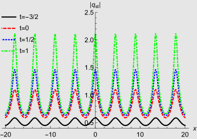
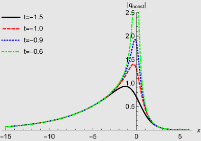
Figure 4: Nonlocal regular one-soliton solution (74) for the nonlocal Hirota equations obtained from the standard Hirota method at different times for $\alpha=0.4$, $\delta=0.8$, $\gamma=0.6+i1.3$ and $\mu=i0.7$, $\lambda=i1.7$ (left panel). Nonlocal rogue wave one-soliton solution (75) for the nonlocal Hirota equations obtained from the nonstandard Hirota method at different times for $\alpha=0.4$, $\delta=1.8$, $\gamma=0.5$, $\theta=0.1$, $\mu=0.2$ and $\nu=1.2$ (right panel).

Notice that for $\alpha\rightarrow-1$ and $\delta\rightarrow 0$ the system (15) reduces to the nonlocal NLSE studied in [17]. For this case the solution (73) acquires exactly the form of equation (22) in [17] when we set $\nu\rightarrow-2\eta_{1}$, $\mu\rightarrow-2\eta_{2}$, $\gamma\rightarrow\theta_{2}$ and $\theta\rightarrow\theta_{1}$. There is no equivalent solution to the regular solution (71) reported in [17], so that $q_{\text{st}}^{(1)}$ for $\delta\rightarrow 0$ is a also new solution for the nonlocal NLSE.

4.1.2 The two-parameter two-soliton solution

As in the local case we expand our auxiliary functions two orders further in order to construct the two-soliton solution. Using the truncated expansions

$$f=1+\varepsilon^{2}f_{2}+\varepsilon^{4}f_{4},\qquad g=\varepsilon g_{1}+\varepsilon^{3}g_{3},\qquad h=\varepsilon h_{1}+\varepsilon^{3}h_{3},$$ (77)

to solve the bilinear equations (62) and (64), we find

$$g_{1} = \tau_{\mu,\gamma}+\tau_{\nu,\delta},$$ (78)

$$g_{3} = \frac{\left(\mu-\nu\right)^{2}}{\left(\mu-\mu^{\ast}\right)^{2}\left(\nu-\mu^{\ast}\right)^{2}}\tau_{\mu,\gamma}\tau_{\nu,\delta}\tilde{\tau}_{\mu,\gamma}^{\ast}+\frac{\left(\mu-\nu\right)^{2}}{\left(\mu-\nu^{\ast}\right)^{2}\left(\nu-\nu^{\ast}\right)^{2}}\tau_{\mu,\gamma}\tau_{\nu,\delta}\tilde{\tau}_{\nu,\delta}^{\ast},$$ (79)

$$f_{2} = \frac{\tau_{\mu,\gamma}\tilde{\tau}_{\mu,\gamma}^{\ast}}{\left(\mu-\mu^{\ast}\right)^{2}}+\frac{\tau_{\nu,\delta}\tilde{\tau}_{\mu,\gamma}^{\ast}}{\left(\nu-\mu^{\ast}\right)^{2}}+\frac{\tau_{\mu,\gamma}\tilde{\tau}_{\nu,\delta}^{\ast}}{\left(\mu-\nu^{\ast}\right)^{2}}+\frac{\tau_{\nu,\delta}\tilde{\tau}_{\nu,\delta}^{\ast}}{\left(\nu-\nu^{\ast}\right)^{2}},$$ (80)

$$f_{4} = \frac{\left(\mu-\nu\right)^{2}\left(\mu^{\ast}-\nu^{\ast}\right)^{2}}{\left(\mu-\mu^{\ast}\right)^{2}\left(\nu-\mu^{\ast}\right)^{2}\left(\mu-\nu^{\ast}\right)^{2}\left(\nu-\nu^{\ast}\right)^{2}}\tau_{\mu,\gamma}\tilde{\tau}_{\mu,\gamma}^{\ast}\tau_{\nu,\delta}\tilde{\tau}_{\nu,\delta}^{\ast},$$ (81)

$$h_{1} = 2\tilde{\tau}_{\mu,\gamma}^{\ast}+2\tilde{\tau}_{\nu,\delta}^{\ast},$$ (82)

$$h_{3} = \frac{2\left(\mu^{\ast}-\nu^{\ast}\right)^{2}}{\left(\mu-\mu^{\ast}\right)^{2}\left(\nu^{\ast}-\mu\right)^{2}}\tilde{\tau}_{\mu,\gamma}^{\ast}\tilde{\tau}_{\nu,\delta}^{\ast}\tau_{\mu,\gamma}+\frac{2\left(\mu^{\ast}-\nu^{\ast}\right)^{2}}{\left(\mu^{\ast}-\nu\right)^{2}\left(\nu-\nu^{\ast}\right)^{2}}\tilde{\tau}_{\mu,\gamma}^{\ast}\tilde{\tau}_{\nu,\delta}^{\ast}\tau_{\nu,\delta}.$$ (83)

So that for $\varepsilon=1$ we obtain from (78)-(83) the two-soliton solution

$$q_{\text{nl}}^{(2)}(x,t)=\frac{g_{1}(x,t)+g_{3}(x,t)}{1+f_{2}(x,t)+f_{4}(x,t)}$$ (84)

As for the one-soliton solution (71) we recover the solutions to the local equation by taking $\tilde{\tau}\rightarrow\tau$ and $\mu^{\ast}\rightarrow-\mu^{\ast}$, $\nu^{\ast}\rightarrow-\nu^{\ast}$ in the pre-factors. In figure 5 we depict the solution (84) at different times.

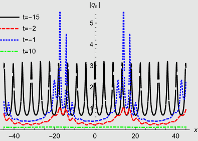
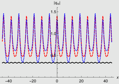
Figure 5: Nonlocal regular two-soliton solution (84) for the nonlocal Hirota equations obtained from the standard Hirota method at different times for $\alpha=0.4$, $\delta=0.8$, $\gamma_{1}=0.6+i1.3$, $\mu_{1}=i0.7$, $\gamma_{2}=0.9+i0.7$, $\mu_{2}=i0.9$ (left panel). Nonlocal regular two one-soliton solution (71) for the nonlocal Hirota equations $\gamma_{1}=0.6+i1.3$, $\mu_{1}=i0.7$ and $\gamma_{2}=0.9+i0.7$, $\mu_{2}=i0.9$ versus the nonlocal regular two-soliton solution (84) at the same values at time $t=2.5$ (right panel).

In the left panel we observe the evolution of the two-soliton solution producing a complicated nonlocal pattern. In the right panel we can see that at large time the two-soliton solutions appears to be an interference between two nonlocal one-solitons.

As in the construction for the one-soliton solutions we can also pursue the option to solve equation (69) only for $\varepsilon=1$ leading to a second type of two-soliton solutions. We will not report them here, but instead discuss how they emerge when using Darboux-Crum transformations.

4.2 Darboux-Crum transformations

We start again by choosing the vanishing seed functions $q=r=0$ and solve the linear equations (2) with $\lambda\rightarrow i\lambda$, i.e. (55), with the additional constraint $\beta=i\delta$ by

$$\tilde{\Psi}_{1}(x,t;\lambda)=\left(\begin{array}[]{c}\varphi_{1}(x,t;\lambda)\\ \phi_{1}(x,t;\lambda)\end{array}\right)=\left(\begin{array}[]{c}e^{\lambda x+2i\lambda^{2}(\alpha-2\delta\lambda)t+\gamma_{1}}\\ e^{-\lambda x-2i\lambda^{2}(\alpha-2\delta\lambda)t+\gamma_{2}}\end{array}\right).$$ (85)

In the construction of $\Psi_{2}$ we implement now the constraint $r(x,t)=\pm q^{\ast}(-x,t)$, with $\kappa=\pm 1$, that gives rise to the nonlocal equations (15) and (16). As suggested from the previous section we expect to obtain two different types of solutions. Indeed, unlike as in the local case we have now two options at our disposal to enforce the constraint. The standard choice consists of taking $\varphi_{2}=\pm\tilde{\phi}_{1}^{\ast}$, $\phi_{2}=\tilde{\varphi}_{1}^{\ast}$ for complex parameters which is very similar to the approach in local case. Alternatively we can choose here $\phi_{1}=\tilde{\varphi}_{1}^{\ast}$, $\phi_{2}=\pm\tilde{\varphi}_{2}^{\ast}$. Evidently the first equation in the latter constraint holds when $\gamma_{2}^{\ast}=\gamma_{1}$ in (85). It is also clear that the second option is not available in the local case.

For the first choice we obtain therefore

$$\tilde{\Psi}_{2}(x,t;\lambda)=\left(\begin{array}[]{c}\varphi_{2}(x,t;\lambda)\\ \phi_{2}(x,t;\lambda)\end{array}\right)=\left(\begin{array}[]{c}\mp\phi_{1}^{\ast}(-x,t;\lambda)\\ \varphi_{1}^{\ast}(-x,t;\lambda)\end{array}\right)=\left(\begin{array}[]{c}\mp e^{\lambda^{\ast}x+2i(\lambda^{\ast})^{2}(\alpha-2\delta\lambda)t+\gamma_{2}^{\ast}}\\ e^{-\lambda^{\ast}x-2i(\lambda^{\ast})^{2}(\alpha-2\delta\lambda^{\ast})t+\gamma_{1}^{\ast}}\end{array}\right),$$ (86)

with $\lambda$,$\gamma_{1},\gamma_{2}\in\mathbb{C}$ and hence for the lower sign with (50) we have

$$q_{\text{st}}^{(1)}(x,t)=\frac{2(\text{$\lambda$}^{\ast}-\lambda)e^{2\text{$\lambda$}^{\ast}x+2i(\text{$\lambda$}^{\ast})^{2}(\alpha-2\delta\text{$\lambda$}^{\ast})t-\text{$\gamma$}_{1}^{\ast}+\text{$\gamma$}_{2}^{\ast}}}{1+e^{2(\text{$\lambda$}^{\ast}-\lambda)x+4i\left[\alpha(\text{$\lambda$}^{\ast})^{2}-\alpha\lambda^{2}+2\delta\lambda^{3}-2\delta(\text{$\lambda$}^{\ast})^{3}\right]t-\gamma_{1}+\gamma_{2}-\text{$\gamma$}_{1}^{\ast}+\text{$\gamma$}_{2}^{\ast}}}.$$ (87)

For the second choice we take $\Psi_{1}(x,t;\mu)$ with $\mu\in\mathbb{R}$ and $\gamma_{2}=\gamma_{1}^{\ast}$ in (85). In this choice the second wavefunction decouples entirely from the first and we may therefore also choose different parameters. Again for the lower  we take

$$\tilde{\Psi}_{2}(x,t;\nu)=\left(\begin{array}[]{c}\varphi_{2}(x,t;\nu)\\ \phi_{2}(x,t;\nu)\end{array}\right)=\left(\begin{array}[]{c}e^{\nu x+2i\nu^{2}(\alpha-2\delta\nu)t+\gamma_{3}}\\ -e^{-\nu x-2i\nu^{2}(\alpha-2\delta\nu)t+\gamma_{3}^{\ast}}\end{array}\right)$$ (88)

and hence (50) yields

$$q_{\text{nonst}}^{(1)}(x,t)=\frac{2(\nu-\mu)e^{\gamma_{1}-\gamma_{1}^{\ast}+2\mu x+4i\mu^{2}(\alpha-2\delta\mu)t}}{1+e^{2(\mu-\nu)x+4i(\alpha\mu^{2}-\alpha\nu^{2}-2\delta\mu^{3}+2\delta\nu^{3})t+\gamma_{1}-\gamma_{1}^{\ast}-\gamma_{3}+\gamma_{3}^{\ast}}}.$$ (89)

The $n$-soliton solutions are obtained considering the set

$$\tilde{S}_{2n}^{\text{st}}=\left\{\tilde{\Psi}_{1}(x,t;\lambda_{1}),\tilde{\Psi}_{2}(x,t;\lambda_{1}),\tilde{\Psi}_{1}(x,t;\lambda_{2}),\tilde{\Psi}_{2}(x,t;\lambda_{2}),...,\tilde{\Psi}_{1}(x,t;\lambda_{n}),\tilde{\Psi}_{2}(x,t;\lambda_{n})\right\}$$ (90)

or

$$\tilde{S}_{2n}^{\text{nonst}}=\left\{\tilde{\Psi}_{1}(x,t;\mu_{1}),\tilde{\Psi}_{2}(x,t;\nu_{1}),\tilde{\Psi}_{1}(x,t;\mu_{2}),\tilde{\Psi}_{2}(x,t;\nu_{2}),...,\tilde{\Psi}_{1}(x,t;\mu_{n}),\tilde{\Psi}_{2}(x,t;\nu_{n})\right\}$$ (91)

with (85) and (86) and the formulae (51).

5 The nonlocal complex time-reversed Hirota equation

In this case the compatibility between the equations (10) and (11) is achieved by the choice $r(x,t)=\pm q^{\ast}(x,-t)$ when taking $\kappa=\pm 1$. As $t$ is directly related to $-t$, we expect some nonlocality in time to emerge in this model. Since it is now clear how the two different types of solutions emerge within the context of the Hirota method as well as in the application of the Darboux-Crum transformations, we report here only the latter scenario. Using vanishing seed functions $q=r=0$ we solve the linear equations (2) with $\lambda\rightarrow i\lambda$, $\alpha=i\hat{\delta}$ and $\beta=i\delta$ by

$$\hat{\Psi}_{1}(x,t;\lambda)=\left(\begin{array}[]{c}\varphi_{1}(x,t;\lambda)\\ \phi_{1}(x,t;\lambda)\end{array}\right)=\left(\begin{array}[]{c}e^{\lambda x-2\lambda^{2}(\hat{\delta}+2i\delta\lambda)t+\gamma_{1}}\\ e^{-\lambda x+2\lambda^{2}(\hat{\delta}+2i\delta\lambda)t+\gamma_{2}}\end{array}\right).$$ (92)

The constraint $r(x,t)=\pm\hat{q}^{\ast}(x,-t)$ in (50) can be implemented in two different ways by either taking $\varphi_{2}=\pm\hat{\phi}_{1}^{\ast}$, $\phi_{2}=\hat{\varphi}_{1}^{\ast}$ obtaining

$$\hat{\Psi}_{2}(x,t;\lambda)=\left(\begin{array}[]{c}\varphi_{2}(x,t;\lambda)\\ \phi_{2}(x,t;\lambda)\end{array}\right)=\left(\begin{array}[]{c}\pm\phi_{1}^{\ast}(x,-t;\lambda)\\ \varphi_{1}^{\ast}(x,-t;\lambda)\end{array}\right)=\left(\begin{array}[]{c}\pm e^{-\lambda^{\ast}x-2(\lambda^{\ast})^{2}(\hat{\delta}-2i\delta\lambda^{\ast})t+\gamma_{2}^{\ast}}\\ e^{\lambda^{\ast}x+2(\lambda^{\ast})^{2}(\hat{\delta}-2i\delta\lambda^{\ast})t+\gamma_{1}^{\ast}}\end{array}\right),$$ (93)

or $\phi_{1}=\hat{\varphi}_{1}^{\ast}$, $\phi_{2}=\pm\hat{\varphi}_{2}^{\ast}$ with $\lambda=\mu\in i\mathbb{R}$, $\gamma_{2}=\gamma_{1}^{\ast}$ and new constants $\nu\in i\mathbb{R}$, $\gamma_{2}\in\mathbb{C}$ so that we have

$$\hat{\Psi}_{2}(x,t;\nu)=\left(\begin{array}[]{c}\pm\varphi_{2}(x,t;\nu)\\ \phi_{2}(x,t;\nu)\end{array}\right)=\left(\begin{array}[]{c}\pm e^{\nu x-2\nu^{2}(\hat{\delta}+2i\delta\nu)t+\gamma_{2}}\\ e^{-\nu x+2\nu^{2}(\hat{\delta}+2i\delta\nu)t+\gamma_{2}^{\ast}}\end{array}\right).$$ (94)

The corresponding one-soliton solutions computed with (50) are therefore

$$q_{\text{st}}^{(1)}(x,t)=\frac{\pm 2(\lambda+\lambda^{\ast})e^{2\lambda x+\gamma_{1}+\text{$\gamma$}_{2}^{\ast}}}{e^{2x(\lambda+\lambda^{\ast})+4(\lambda^{\ast})^{2}(\hat{\delta}-2i\delta\lambda^{\ast})t+\gamma_{1}+\text{$\gamma$}_{1}^{\ast}}\mp e^{4\lambda^{2}(\hat{\delta}+2i\delta\lambda)t+\gamma_{2}+\text{$\gamma$}_{2}^{\ast}}},$$ (95)

and

$$q_{\text{nonst}}^{(1)}(x,t)=\frac{\pm 2(\mu-\nu)e^{2x(\mu+\nu)+\gamma_{1}+\gamma_{2}}}{e^{2\mu x+4\nu^{2}(\hat{\delta}+2i\delta\nu)t+\gamma_{1}+\text{$\gamma$}_{2}^{\ast}}\mp e^{2\nu x+4\mu^{2}(\hat{\delta}+2i\delta\mu)t+\gamma_{2}+\text{$\gamma$}_{1}^{\ast}}}.$$ (96)

The nonlocality is now only felt in time for fixed values of $x$, but we expect to find well localized solutions in space for fixed values of $t$. It is clear how to compute the $n$-soliton solutions, simply by using the set

$$\hat{S}_{2n}^{\text{st}}=\left\{\hat{\Psi}_{1}(x,t;\lambda_{1}),\hat{\Psi}_{2}(x,t;\lambda_{1}),\hat{\Psi}_{1}(x,t;\lambda_{2}),\hat{\Psi}_{2}(x,t;\lambda_{2}),...,\hat{\Psi}_{1}(x,t;\lambda_{n}),\hat{\Psi}_{2}(x,t;\lambda_{n})\right\}$$ (97)

or

$$\hat{S}_{2n}^{\text{nonst}}=\left\{\hat{\Psi}_{1}(x,t;\mu_{1}),\hat{\Psi}_{2}(x,t;\nu_{1}),\hat{\Psi}_{1}(x,t;\mu_{2}),\hat{\Psi}_{2}(x,t;\nu_{2}),...,\hat{\Psi}_{1}(x,t;\mu_{n}),\hat{\Psi}_{2}(x,t;\nu_{n})\right\}$$ (98)

with (92) and (93) and the formulae (51).

An interesting special case is obtained for $\hat{\delta}=0$, which correspond to a complex nonlocal time-reverse version of the modified KdV equation. In this case the solution (95) has no poles for the lower sign and is asymptotically finite for $t\rightarrow\pm\infty$ as long as $\mathop{\mathrm{R}e}\gamma_{1}\neq 0$ and $\mathop{\mathrm{R}e}\gamma_{2}\neq 0$. We depict some one and two-soliton solutions for the case in figure 6.

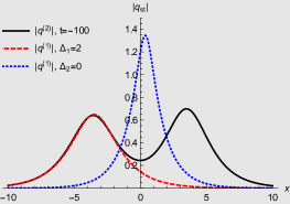
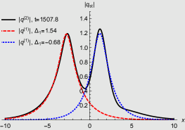
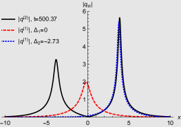
Figure 6: Modulus of two one-soliton solutions (95) and the corresponding two-soliton solutions for the complex nonlocal time-reverse version of the modified KdV equation at $\hat{\delta}=0$, $\delta=1.0$ and different values of time. The one-solitons are computed at for $\lambda=0.3$, $\gamma_{1}=0.3+\Delta_{1}$ $\gamma_{2}=0.2$ and $\lambda=0.4$, $\gamma_{1}=0.2+\Delta_{2}$ $\gamma_{2}=0.5$. The two-soliton is computed for the same values with $\Delta_{1}=\Delta_{2}=0$.

We observe from the local nature of the solutions in space and the feature that the two-soliton solution has one-soliton constituents. As shown in figure 6 when shifting the parameters in the one-soliton solutions appropriately they match exactly the one-soliton constituents in the two-soliton solution. However, this only happens at special instances in time and the solutions will not keep oscillating in synchronicity when time evolves, even for large values of time.

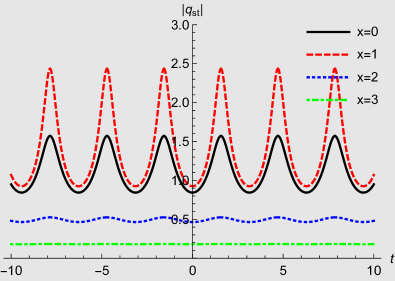
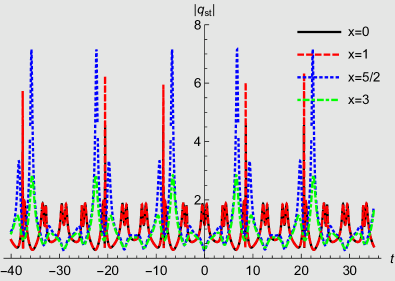
Figure 7: Time crystal structures in the complex nonlocal time-reverse version of the modified KdV equation at $\hat{\delta}=0$, $\delta=1.0$ and different points in space. The one-soliton solutions (95) are computed for $\lambda=0.5$, $\gamma_{1}=0.2$ and $\gamma_{2}=0.8$ (left panel). The two-soliton solutions are computed at for $\lambda_{1}=0.6$, $\gamma_{1}=0.2$, $\gamma_{2}=0.8$, $\lambda_{2}=0.3$, $\gamma_{3}=0.2$ and $\gamma_{4}=0.5$ (right panel).

The nonlocality is now in time, displaying a time crystal [38, 39] like structure as seen in figure 7.

6 The nonlocal complex $\mathcal{PT}$-transformed Hirota equation

In this case the compatibility between the equation (10) and (11) is achieved by the choice $r(x,t)=\pm q^{\ast}(-x,-t)$ when taking $\kappa=\pm 1$. As $x$ and $t$ are now directly related to $-x$ and $-t$, we expect some nonlocality to emerge in space as well as in time. With seed functions $q=r=0$, $\alpha=i\check{\delta}$, $\check{\delta},\beta\in\mathbb{R}$ we solve the linear equations (2) by

$$\check{\Psi}_{1}(x,t;\lambda)=\left(\begin{array}[]{c}\varphi_{1}(x,t;\lambda)\\ \phi_{1}(x,t;\lambda)\end{array}\right)=\left(\begin{array}[]{c}e^{\lambda x-2\lambda^{2}(\check{\delta}+2\beta\lambda)t+\gamma_{1}}\\ e^{-\lambda x+2\lambda^{2}(\check{\delta}+2\beta\lambda)t+\gamma_{2}}\end{array}\right).$$ (99)

Implementing the constraint $r(x,t)=\pm q^{\ast}(-x,-t)$ in (50) by $\varphi_{2}=\pm\check{\phi}_{1}^{\ast}$, $\phi_{2}=\check{\varphi}_{1}^{\ast}$ we obtain

$$\check{\Psi}_{2}(x,t;\lambda)=\left(\begin{array}[]{c}\varphi_{2}(x,t;\lambda)\\ \phi_{2}(x,t;\lambda)\end{array}\right)=\left(\begin{array}[]{c}\mp\phi_{1}^{\ast}(-x,-t;\lambda)\\ \varphi_{1}^{\ast}(-x,-t;\lambda)\end{array}\right)=\left(\begin{array}[]{c}\mp e^{-\lambda^{\ast}x-2(\lambda^{\ast})^{2}(\check{\delta}+2\beta\lambda^{\ast})t+\gamma_{2}^{\ast}}\\ e^{\lambda^{\ast}x+2(\lambda^{\ast})^{2}(\check{\delta}+2\beta\lambda^{\ast})t+\gamma_{1}^{\ast}}\end{array}\right),$$ (100)

or $\phi_{1}=\check{\varphi}_{1}^{\ast}$, $\phi_{2}=-\check{\varphi}_{2}^{\ast}$ with $\lambda=\mu\in\mathbb{R}$, $\gamma_{2}=\gamma_{1}^{\ast}$ and new constants $\nu\in\mathbb{R}$, $\gamma_{2}\in\mathbb{C}$ we have

$$\check{\Psi}_{2}(x,t;\nu)=\left(\begin{array}[]{c}-\varphi_{2}(x,t;\nu)\\ \phi_{2}(x,t;\nu)\end{array}\right)=\left(\begin{array}[]{c}-e^{\nu x-2\nu^{2}(\check{\delta}+2\beta\nu)t+\gamma_{2}}\\ e^{-\nu x+2\nu^{2}(\check{\delta}+2\beta\nu)t+\gamma_{2}^{\ast}}\end{array}\right).$$ (101)

The corresponding one-soliton solutions computed with (50) are therefore

$$q_{\text{st}}^{(1)}(x,t)=\frac{\pm 2(\lambda-\lambda^{\ast})e^{\gamma_{1}+\text{$\gamma$}_{2}^{\ast}+2(\lambda+\lambda^{\ast})x}}{e^{\gamma_{1}+\text{$\gamma$}_{1}^{\ast}+4(\lambda^{\ast})^{2}(2\beta\lambda^{\ast}+\check{\delta})t+2\mu x}\pm e^{\gamma_{2}+\text{$\gamma$}_{2}^{\ast}+4\lambda\mu^{2}(2\beta\lambda+\check{\delta})t+2\lambda^{\ast}x}},$$ (102)

and

$$q_{\text{nonst}}^{(1)}(x,t)=\frac{2(\nu-\mu)e^{\gamma_{1}-\text{$\gamma$}_{1}^{\ast}+2(\mu+\nu)x}}{e^{4\mu^{2}(2\beta\mu+\check{\delta})t+2\nu x}+e^{4\nu^{2}(2\beta\nu+\check{\delta})t+2\mu x}}.$$ (103)

With (99) and (100) in the sets

$$\check{S}_{2n}^{\text{st}}=\left\{\check{\Psi}_{1}(x,t;\lambda_{1}),\check{\Psi}_{2}(x,t;\lambda_{1}),\check{\Psi}_{1}(x,t;\lambda_{2}),\check{\Psi}_{2}(x,t;\lambda_{2}),...,\check{\Psi}_{1}(x,t;\lambda_{n}),\check{\Psi}_{2}(x,t;\lambda_{n})\right\}$$ (104)

or

$$\check{S}_{2n}^{\text{nonst}}=\left\{\check{\Psi}_{1}(x,t;\mu_{1}),\check{\Psi}_{2}(x,t;\nu_{1}),\check{\Psi}_{1}(x,t;\mu_{2}),\check{\Psi}_{2}(x,t;\nu_{2}),...,\check{\Psi}_{1}(x,t;\mu_{n}),\check{\Psi}_{2}(x,t;\nu_{n})\right\}$$ (105)

the $n$-soliton solutions are computed from the formulae (51).

As discussed above, the choices $r(x,t)=\pm q(-x,t)$ and $r(x,t)=\pm q(x,-t)$ with real $q$s are less interesting and will therefore not discuss the here.

7 The nonlocal conjugate $\mathcal{PT}$-transformed Hirota equation

In this case the compatibility between the equation (10) and (11) is achieved by the choice $r(x,t)=\kappa q(-x,-t)$ with $\kappa\in\mathbb{C}$. As in the previous section we take $q=r=0$, but with no further restrictions on the parameters involved and solve the linear equations (2) to

$$\check{\Psi}_{1}(x,t;\lambda)=\left(\begin{array}[]{c}\varphi_{1}(x,t;\lambda)\\ \phi_{1}(x,t;\lambda)\end{array}\right)=\left(\begin{array}[]{c}e^{\lambda x+2\lambda^{2}(i\alpha-2\beta\lambda)t+\gamma_{1}}\\ e^{-\lambda x-2\lambda^{2}(i\alpha-2\beta\lambda)t+\gamma_{2}}\end{array}\right).$$ (106)

When implementing the constraint $r(x,t)=\kappa q(-x,-t)$ in (50) by $\varphi_{2}=\kappa\check{\phi}_{1}^{\ast}$, $\phi_{2}=\check{\varphi}_{1}^{\ast}$ we obtain a $\Psi_{2}(x,t;\lambda)$ leading to $\det D_{1}^{q}=\det D_{1}^{r}=0$ so that the standard solution does not exist in this case. However, implementing $\phi_{1}=i\sqrt{\kappa}\check{\varphi}_{1}$, by taking $e^{\gamma_{2}}=i\sqrt{\kappa}e^{\gamma_{1}}$, $\lambda\rightarrow\mu$ and likewise for $\phi_{2}=-i\sqrt{\kappa}\check{\varphi}_{2}$ with new spectral parameters $\lambda\rightarrow\nu$ and shift parameter $\gamma_{3}=\gamma_{1}$ we obtain

$$q_{\text{nonst}}^{(1)}(x,t)=\frac{2i(\mu-\nu)e^{2\mu x+4i\mu^{2}(\alpha+2i\beta\mu)t}}{\sqrt{\kappa}\left[1+e^{2x(\mu-\nu)+\left[4i\alpha(\mu^{2}-\nu^{2})+8\beta(\nu^{3}-\mu^{3})\right]t}\right]}.$$ (107)

We notice that all shift parameters have cancelled and since $x$ and $t$ are real the solution is in general regular. Interestingly, since the compatibility requirement between (10) and (11) does not involve a conjugation, we shift formally shift $x$ and $t$ by any complex value, which means that $q_{\text{nonst}}^{(1)}(x+\Delta_{1},t+\Delta_{2})$ with $\Delta_{1},\Delta_{2}\in\mathbb{C}$ is also a solution that will, however, in general not satisfy the constraint $r(x,t)=\kappa q(-x,-t)$. Note that this operation does not constitute a full variable substitution, i.e. the differentials are not replaced. The $n$-soliton solutions are obtained by using the set

$$\check{S}_{2n}^{\text{nonst}}=\left\{\check{\Psi}_{1}(x,t;\mu_{1}),\check{\Psi}_{2}(x,t;\nu_{1}),\check{\Psi}_{1}(x,t;\mu_{2}),\check{\Psi}_{2}(x,t;\nu_{2}),...,\check{\Psi}_{1}(x,t;\mu_{n}),\check{\Psi}_{2}(x,t;\nu_{n})\right\},$$ (108)

in the formulae (51).

8 Conclusions

We exploited various possibilities involving different combinations of parity, time-reversal and complex conjugation to achieve compatibility between the two equations (10) and (11) resulting from the zero curvature condition for the Hirota equation. Each possibility corresponds to a new type of integrable system. Solving these new nonlocal equations by means of Hirota’s direct method we encountered various new features. Instead of having to solve two bilinear equations, these new systems correspond to three bilinear equations involving an auxiliary function. We solved these equations in the standard fashion by using a formal expansion parameter that in the end can be set to any value when the expansions are truncated at specific orders. In addition, the new auxiliary equation allows for a new option for this equation to be solve for a specific value of the expansion parameter, thus leading to a new type of solution different from the one obtained in the standard fashion. We also identified the mechanism leading to this second type of solution within the approach of using Darboux-Crum transformations. In that context the nonlocal relations between $q$ and $r$ allow for different options in (50).

We have found various different type of behaviours. For the local Hirota equation the sign of the parameter $\kappa$ determines whether the solutions are regular or singular whereas tuning the spectral parameter can produce two soliton solutions with a faster one overtaking a slower one, a head-on collision and, most interestingly, a solution in which one of the solitons behaves like a defect. The nonlocal complex parity transformed Hirota equation has two different types of solutions displaying a nonlocal structure of periodically distributed static breathers or rogue waves. The nonlocal complex time-reversed Hirota equation possesses regular localized solutions in space, but is nonlocal in time displaying some time crystal like structures.

There are various interesting questions left for exploration. Evidently more concrete scenario for the above cases can be explored and further solutions may be constructed, for instance by taking different seed function in the Darboux-Crum transformation etc. We also left aside the study of further interesting properties, such as degeneracies, time-delays etc., which were considered in [40, 32, 33, 34]. As the approach we followed is general, further new models related to integrable or even nonintegerable realizations of HNLSE (1) other than the Hirota equation can be constructed and possibly different types of systems altogether. The most interesting challenge is to investigate whether these nonlocal solutions can be realized experimentally.

Acknowledgments: JC is supported by a City, University of London Research Fellowship. FC was partially supported by Fondecyt grant 1171475. AF would like to thank the Instituto de Ciencias Físicas y Matemática at the Universidad Austral de Chile for kind hospitality.

References

- [1] A. Shabat and V. Zakharov, Exact theory of two-dimensional self-focusing and one-dimensional self-modulation of waves in nonlinear media, Sov. Phys. JETP 34(1), 62–69 (1972).
- [2] G. P. Agrawal, Fiber-optic communication systems, volume 222, John Wiley & Sons, 2012.
- [3] P. K. Shukla and B. Eliasson, Nonlinear aspects of quantum plasma physics, Physics-Uspekhi 53(1), 51–76 (2010).
- [4] L. F. Mollenauer, R. H. Stolen, and J. P. Gordon, Experimental observation of picosecond pulse narrowing and solitons in optical fibers, Phys. Rev. Lett. 45(13), 1095 (1980).
- [5] F. M. Mitschke and L. F. Mollenauer, Discovery of the soliton self-frequency shift, Optics Letters 11(10), 659–661 (1986).
- [6] J. P. Gordon, Theory of the soliton self-frequency shift, Optics letters 11(10), 662–664 (1986).
- [7] Y. Kodama and A. Hasegawa, Nonlinear pulse propagation in a monomode dielectric guide, IEEE Journal of Quantum Electronics 23(5), 510–524 (1987).
- [8] D. Anderson and M. Lisak, Nonlinear asymmetric self-phase modulation and self-steepening of pulses in long optical waveguides, Phys. Rev. A 27(3), 1393 (1983).
- [9] H. Chen, Y. Lee, and C. Liu, Integrability of nonlinear Hamiltonian systems by inverse scattering method, Physica Scripta 20(3-4), 490 (1979).
- [10] M. Wadati and K. Sogo, Gauge transformations in soliton theory, J. Phys. Soc. Japan 52(2), 394–398 (1983).
- [11] N. Sasa and J. Satsuma, New-type of soliton solutions for a higher-order nonlinear Schrödinger equation, J. Phys. Soc. Japan 60(2), 409–417 (1991).
- [12] R. Hirota, Exact envelope-soliton solutions of a nonlinear wave equation, J. Math. Phys. 14(7), 805–809 (1973).
- [13] A. Fring, PT-symmetric deformations of integrable models, Phil. Trans. Royal Soc. London A: Math., Phys. and Eng. Sci. 371(1989), 20120046 (2013).
- [14] F. K. Abdullaev, Y. V. Kartashov, V. V. Konotop, and D. A. Zezyulin, Solitons in PT-symmetric nonlinear lattices, Phys. Rev. A 83(4), 041805 (2011).
- [15] N. V. Alexeeva, I. Barashenkov, A. A. Sukhorukov, and Y. S. Kivshar, Optical solitons in PT-symmetric nonlinear couplers with gain and loss, Phys. Rev. A 85(6), 063837 (2012).
- [16] V. V. Konotop, J. Yang, and D. A. Zezyulin, Nonlinear waves in PT-symmetric systems, Rev. of Mod. Phys. 88(3), 035002 (2016).
- [17] M. J. Ablowitz and Z. H. Musslimani, Integrable nonlocal nonlinear Schrödinger equation, Phys. Rev. Lett. 110(6), 064105 (2013).
- [18] M. J. Ablowitz and Z. H. Musslimani, Integrable nonlocal nonlinear equations, Studies in Applied Mathematics (2016).
- [19] J. Weiss, M. Tabor, and G. Carnevale, The Painlevé property for partial differential equations, J. Math. Phys. 24, 522–526 (1983).
- [20] J. Weiss, The Painlevé property for partial differential equations. II: Bäcklund transformation, Lax pairs, and the Schwarzian derivative, J. Math. Phys. 24, 1405–1413 (1983).
- [21] P. Lax, Integrals of nonlinear equations and solitary waves, Commun. Pure Appl. Math. 21, 467–490 (1968).
- [22] M. J. Ablowitz, D. J. Kaup, A. C. Newell, and H. Segur, Nonlinear-evolution equations of physical significance, Phys. Rev. Lett. 31(2), 125 (1973).
- [23] R. Hirota, The direct method in soliton theory, volume 155, Cambridge University Press, 2004.
- [24] W.-J. Liu, B. Tian, H.-Q. Zhang, L.-L. Li, and Y.-. Xue, Soliton interaction in the higher-order nonlinear Schrödinger equation investigated with Hirota’s bilinear method, Phys. Rev. E 77(6), 066605 (2008).
- [25] J. Hietarinta, A search for bilinear equations passing Hirota’s three-soliton condition. IV. Complex bilinear equations, J. Math. Phys. 29(3), 628–635 (1988).
- [26] J. Eggers, Air entrainment through free-surface cusps, Phys. Rev. Lett. 86(19), 4290(4) (2001).
- [27] G. Darboux, On a proposition relative to linear equations, physics/9908003, Comptes Rendus Acad. Sci. Paris 94, 1456–59 (1882).
- [28] M. M. Crum, Associated Sturm-Liouville systems, The Quarterly Journal of Mathematics 6(1), 121–127 (1955).
- [29] V. B. Matveev and M. A. Salle, Darboux transformation and solitons, (Springer, Berlin) (1991).
- [30] L. M. Nieto, A. A. Pecheritsin, and B. F. Samsonov, Intertwining technique for the one-dimensional stationary Dirac equation, Annals. of Phys. 305(2), 151–189 (2003).
- [31] F. Correa and V. Jakubskỳ, Confluent Crum-Darboux transformations in Dirac Hamiltonians with PT-symmetric Bragg gratings, Phys. Rev. A 95(3), 033807 (2017).
- [32] F. Correa and A. Fring, Regularized degenerate multi-solitons, Journal of High Energy Physics 2016(9), 8 (2016).
- [33] J. Cen, F. Correa, and A. Fring, Time-delay and reality conditions for complex solitons, J. of Math. Phys. 58(3), 032901 (2017).
- [34] J. Cen, F. Correa, and A. Fring, Degenerate multi-solitons in the sine-Gordon equation, J. Phys. A: Math. Theor. 50, 435201 (2017).
- [35] S. Stalin, M. Senthilvelan, and M. Lakshmanan, Nonstandard bilinearization of PT-invariant nonlocal nonlinear Schrödinger equation: Bright soliton solutions, Phys. Lett. A 381(30), 2380–2385 (2017).
- [36] C. Kharif and E. Pelinovsky, Physical mechanisms of the rogue wave phenomenon, Euro. J. of Mech.-B/Fluids 22(6), 603–634 (2003).
- [37] A. Chabchoub, N. P. Hoffmann, and N. Akhmediev, Rogue wave observation in a water wave tank, Phys. Rev. Lett. 106(20), 204502 (2011).
- [38] F. Wilczek, Quantum time crystals, Phys. Rev. Lett. 109(16), 160401 (2012).
- [39] A. Shapere and F. Wilczek, Classical time crystals, Phys. Rev. Lett. 109(16), 160402 (2012).
- [40] J. Cen and A. Fring, Complex solitons with real energies, J. Phys. A: Math. Theor. 49(36), 365202 (2016).